| Issue |
A&A
Volume 703, November 2025
|
|
|---|---|---|
| Article Number | A143 | |
| Number of page(s) | 11 | |
| Section | Extragalactic astronomy | |
| DOI | https://doi.org/10.1051/0004-6361/202555441 | |
| Published online | 13 November 2025 | |
A test of Ca II H & K photometry for isolating massive globular clusters below the metallicity floor
1
Department of Astrophysics/IMAPP, Radboud University, PO Box 9010
6500
GL, Nijmegen, The Netherlands
2
Department of Physics & Astronomy, McMaster University, Hamilton, ON, L8S 4M1
Canada
3
Kapteyn Astronomical Institute, University of Groningen, Landleven 12, 9747
AD, Groningen, The Netherlands
⋆ Corresponding author: This email address is being protected from spambots. You need JavaScript enabled to view it.
.
Received:
8
May
2025
Accepted:
10
September
2025
Abstract
Context. The serendipitous discovery of the M31 globular cluster (GC) EXT8 has presented a significant challenge to current theories of GC formation. By finding other GCs similar to EXT8, it should become clear if and/or how EXT8 can fit into our current understanding of GC formation.
Aims. We aim to test the potential of integrated-light narrowband Ca II H & K photometry as a proxy for the metallicity of GCs to be able to provide effective candidate selection for massive GCs below the GC metallicity floor ([Fe/H] ≤ −2.5).
Methods. We investigate the behaviour of two colours involving the CaHK filter employed by the Pristine survey, CaHK-u and CaHK-g, as a function of metallicity through CFHT MegaCam imaging of EXT8 and a wide set of M31 GCs covering the metallicity range −2.9 ≤ [Fe/H] ≤ +0.4. Additionally, we investigate if the CaHK colours are strongly influenced by horizontal branch morphology through available morphology measurements.
Results. In both of the CaHK colours, EXT8 and two other potential GCs below the metallicity floor could be selected from other metal-poor GCs ([Fe/H] ≤ −1.5), with (CaHK − g)o showing the greater metallicity sensitivity. The RMS values of the linear fits to the metal-poor GCs for both colours show an uncertainty of 0.3 dex on metallicity estimations. Comparisons with u − g and g − z/F450W-F850L colours reinforce the notion that CaHK photometry can be used for effective candidate selection, as they reduce false positive selection rates by at least a factor of 2. We find no strong influence of the horizontal branch morphology on the CaHK colours that would interfere with candidate selection, although the assessment is limited by the quantity and quality of available data.
Key words: globular clusters: general / galaxies: individual: M31 / galaxies: star clusters: general
© The Authors 2025
 Open Access article, published by EDP Sciences, under the terms of the Creative Commons Attribution License (https://creativecommons.org/licenses/by/4.0), which permits unrestricted use, distribution, and reproduction in any medium, provided the original work is properly cited.
This article is published in open access under the Subscribe to Open model. This email address is being protected from spambots. You need JavaScript enabled to view it. to support open access publication.
1. Introduction
Observations of Galactic and extragalactic globular clusters (GCs) have shown a lack of GCs with [Fe/H] ≤ −2.5 with respect to the expectations from chemical evolution models or the metallicity distribution of halo stars (e.g. Bond 1981; Carney et al. 1996; Youakim et al. 2020). The halo metallicity distribution of Youakim et al. (2020) suggests that the probability of not observing a GC with [Fe/H] ≤ −2.5 in the Galaxy is around a 0.5 percent. This points to a genuine truncation in the GC metallicity function and has led to the notion of a minimum metallicity for GCs, referred to as the GC metallicity floor, of [Fe/H]min ≈ −2.5 (Forbes et al. 2018; Beasley et al. 2019).
The reason for the metallicity floor remains unclear. A simple explanation is that GCs are unable to form in extremely low-metallicity environments. Possible culprits are the gas fragmentation properties or inefficient cooling expected in such environments (e.g. Loeb & Rasio 1994; Abel et al. 2002). A parallel can be drawn with the G-dwarf problem (van den Bergh 1962), which suggests that the interstellar medium might have already been sufficiently enriched when GCs started forming.
It has also been suggested that the metallicity floor is a natural consequence of the galaxy mass–metallicity relation and the hierarchical nature of galaxy assembly (Kruijssen 2019). In this scenario, the metallicity floor is due to the fact that galaxies with [Fe/H] ≤ −2.5 are not massive enough to form GCs with sufficient mass to avoid total dissolution due to various dynamical effects for up to a Hubble time (estimated at 105 M⊙; Reina-Campos et al. 2018). This scenario is supported by the recent discoveries of two stellar streams, Phoenix ([Fe/H] = −2.7 ± 0.06; Wan et al. 2020) and C-19 ([Fe/H] = −3.38 ± 0.26; Martin et al. 2022), which could be remnants of low-mass GCs (∼104 M⊙). However, we note that the total initial stellar mass of C-19 is uncertain. The rather large observed velocity dispersion and stream width leave a range of possibilities for its progenitor properties (see Errani et al. 2022; Yuan et al. 2022; Viswanathan et al. 2025; Yuan et al. 2025; Carlberg et al. 2025).
Another recent discovery related to the metallicity floor is a serendipitous finding by Larsen et al. (2020). Using a high-S/N and high-resolution spectrum, they found the M31 GC EXT8 to have a metallicity of [Fe/H] = −2.91 ± 0.04 and a mass of 1.1 × 10⁶ M⊙. This combination of extremely low metallicity and high mass is in such stark contrast to the expected combinations from current theory that EXT8 should not exist. A colour-magnitude diagram (CMD) of EXT8 obtained with the Hubble Space Telescope confirmed that it is a genuine old but very metal-poor GC (Larsen et al. 2021). EXT8 and the associated implied existence of massive GCs below the metallicity floor presents a strong challenge to the currently most accepted paradigm of GC formation (Kruijssen 2015).
Such a serendipitous discovery naturally calls for a more structured search to improve the statistics and thus put tighter constraints on possible scenarios for the existence of massive GCs below the metallicity floor. Finding more GCs like EXT8 will, however, be very challenging given the combination of their observed rarity and extremely low metallicity. While accurate metallicity determinations at [Fe/H] ≤ −2 necessitate high-S/N and high-resolution spectra, such observations require a great deal of observing time at current facilities, and an effective way of pre-selecting the most metal-poor candidates is therefore desirable. Traditional broadband photometry becomes increasingly insensitive to metallicity in this regime, but narrowband photometry with carefully chosen filters may provide an effective alternative to more time-consuming spectroscopic observations.
This approach has proven quite successful in the search for the most metal-poor individual stars. In particular, using the Ca II H & K lines for candidate selection has resulted in some of the most successful surveys, such as the HK and Hamburg-ESO surveys (Beers et al. 1992; Christlieb et al. 2008). The Ca II H & K lines even continue to be utilised in modern surveys, such as SkyMapper and Pristine (Keller et al. 2008; Starkenburg et al. 2017). Pristine uses a narrowband filter centred on the Ca II H & K lines, named CaHK, in combination with Sloan Digital Sky Survey (SDSS) or Gaia filters to be able to distinguish metallicities down to [Fe/H] ∼ −3 and has reported a purity of 77 percent for a selection of stars with [Fe/H] ≤ −2.5 (Viswanathan et al. 2025).
This success stems from the fact that the Ca II H & K lines are quite prominent and retain their prominence far better than other metal lines in late-type stars as metallicity decreases (see Fig. 1 from Starkenburg et al. 2017). This allows the Ca II H & K lines to serve as a proxy for metallicity that retains good sensitivity even in the very and extremely metal-poor regimes.
Globular clusters are nearly mono-metallic, and late-type stars constitute a majority of their stellar population. This tentatively suggests that the Ca II H & K lines could also be used as a metallicity indicator to identify very metal-poor GCs.
This potential of Ca II H & K lines has already been noted by Zinn (1980), who upon studying a spectrum of M92 ([Fe/H] = −2.31 dex; Harris 1996, 2010 edition) remarked that the only strong metal lines remaining were the Ca II H & K lines and that they might be the best, and perhaps the only, option for distinguishing a GC more metal-poor than M92 from M92 through integrated light.
With the serendipitous discovery of EXT8 and the challenge it poses to the current ideas about GC formation, the potential of the Ca II H & K lines as a metallicity indicator for metal-poor GCs could be a highly efficient tool in the search for massive GCs below the metallicity floor. We aimed to test this potential by investigating whether EXT8 could be identified through Ca II H & K photometry using the CaHK filter from Pristine. To this end, EXT8 alongside a wide sample of GCs in M31 were imaged in CaHK, u, g, and i by the MegaCam instrument on the Canada-France-Hawaii Telescope (CFHT).
2. Data
The imaging for this study was obtained with MegaCam at the CFHT under programme 22bc04 (PI: Harris). The imaging consists of two fields, seen in Fig. 1 alongside the positions of all GCs from the catalogue of Caldwell & Romanowsky (2016, hereafter C&R16) and reddening values from the Schlegel et al. (1998) dust map. One field lies farther out in the M31 halo and contains EXT8, highlighted in red, alongside a handful of other GCs. The second field lies closer to M31, covering a large portion of the disc and the centre of M31, clearly highlighted by the larger reddening values, encompassing substantially more GCs.
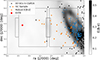 |
Fig. 1. Observational footprint of this study. The GC sample is marked with either orange diamonds or blue circles, signifying GCs with and without robust reddening estimates. EXT8 is marked in red, and the black circles are confirmed M31 GCs from the C&R16 catalogue that were not considered. The background colour is the reddening from the Schlegel et al. (1998) dust map with the correction of Schlafly et al. (2010), clearly highlighting M31 itself. The two rectangles with ‘ears’ are the observed fields that form the footprint for this study. |
For each field, five exposures of 300 seconds in CaHK were obtained to reach a S/N ≳ 40 for a typical GC (half-light radius of 3 pc and half-light luminosity of MV = −7, equivalent to mV ≅ 17.5 at M31). Alongside the CaHK exposures, the fields were also observed in the MegaCam u, g, and i filters. For each of these three filters, three exposures of 30 seconds were obtained per field. The fields were observed on 25 and 26 July 2022 under camera run 22Am07. On both nights, the sky was photometric for the entire observing period. The image quality for each filter remained relatively stable with differences rarely exceeding the pixel scale of MegaCam. The airmass remained stable or decreased slightly across the observing period. The airmass was around ∼1.1 on the first night and ∼1.3 on the second. The observing logs and main parameters of the observing periods can be found in Table A.1.
The GC catalogue presented by C&R16 offers the largest sample of spectroscopically determined metallicities for M31 GCs within the observational footprint, totalling 125 GCs. We purposefully stuck to spectroscopic metallicities, as they are more robust than their photometric counterparts. The C&R16 catalogue did not include a metallicity for EXT8, so the value of [Fe/H] = −2.91 from Larsen et al. (2020) was assumed. This resulted in a sample of 126 GCs spanning a metallicity range −2.9 ≤ [Fe/H] ≤ +0.4.
Of the 126 GCs, only 7 have metallicities below −2. While the sample has a limited amount of very metal-poor GCs, it does contain B157-G212 ([Fe/H] = −2.6 ± 0.3) and B160-G214 ([Fe/H] = −2.8 ± 0.4) that are very metal-poor and potentially lie beneath the metallicity floor, making them very valuable for comparison with EXT8.
The M31 disc presents a significant challenge in the form of differential extinction. This problem has been tackled by earlier studies of the M31 GC system (e.g. Barmby et al. 2000); however, the uncertainty on these reddening estimates, E(B − V), is often high. The estimated uncertainty on the reddening values in the C&R16 catalogue is ±0.1 mag in E(B − V). To minimise using these uncertain reddening estimates, we adopted reddening estimates from more robust sources wherever possible. We drew from either CMDs (Larsen et al. 2021; Federici et al. 2012) or the Schlegel et al. (1998) dust map, with the correction of Schlafly et al. (2010), where E(B − V) ≤ 0.15. For the remaining GCs, we adopted the reddening values from C&R16. The C&R16 catalogue did not possess reddening values for five GCs, which were obtained from either Fan et al. (2010) or Kang et al. (2012).
Values for the extinction coefficients for the MegaCam u, g and i filters have not been published as far as we are aware. It was opted to approximate the extinction coefficients,  , for all filters by considering the filters at their reference wavelength. The Fitzpatrick (1999) extinction law with RV = 3.1 was adopted for the approximations, following the results of Schlafly & Finkbeiner (2011). The resultant extinction coefficients for the four filters can be found in Table 1. The extinction coefficient for CaHK was recently calculated by Martin et al. (2024) and only differs by 0.003 from the value adopted here.
Approximated extinction coefficients for the MegaCam filters.
2.1. Photometry
Each of the exposures had come preprocessed by the Elixir pipeline (Magnier & Cuillandre 2004), which had de-biased, detrended, and flat-fielded them. The background estimation and aperture photometry was done with SourceExtractor version 2.25.0 (Bertin & Arnouts 1996). For background estimation, a combination of BACK_SIZE = (36, 36) and BACK_FILTERSIZE = (8, 8) was used alongside local re-examination around sources (BACKPHOT_TYPE = LOCAL). The size of the box in which the re-examination took place was set to 13 by 13 arcsecond, BACKPHOT_THICK = (70, 70), in order to accommodate the size of the largest GCs in our sample.
As it is expected that GCs do not show colour gradients, it was chosen to use a small static aperture for photometry. The size of the aperture was chosen to match the size of the smallest GCs within the sample to prevent the smallest GCs from being heavily influenced by their backgrounds. Using the g-band aperture sizes from Peacock et al. (2010) as a guideline, the diameter of the aperture was chosen to be 3 arcsecond (11.5 pc). This aperture size is larger than the majority of half-light radii reported by Peacock et al. (2010) for the GCs in our sample.
2.2. Calibration
Calibration of the photometry was done by utilising synthetic photometry derived from the low-resolution Gaia BP and RP (or shortened to XP) spectra through GaiaXPy1 (Gaia Collaboration 2023). The CaHK filter was already available in GaiaXPy but the MegaCam u, g and i filters were not. As broadband filters needed to be ‘standardised’, we used the already standardised SDSS system and transformed them to the MegaCam u, g and i magnitudes following the relation defined in the documentation of the MegaCam filter set2. The synthetic CaHK magnitudes were not standardised but the sample checked by Gaia Collaboration (2023) against Pristine CaHK magnitudes showed that the synthetic CaHK magnitudes only had an offset of 0.04 mag.
To get a clean sample of stars with XP spectra from Gaia DR3, a combination of the re-normalised unit weight error (RUWE) and C* diagnostic metrics were used (Lindegren et al. 2021; Riello et al. 2021). We adopted the cuts of RUWE < 1.4 and |C*| < σ, where σ is the 1σ scatter measured as a power law with magnitude in Riello et al. (2021). Additionally, we adopted a cut of S/N ≥ 30 on the synthetic photometry for u and CaHK, per recommendation of Gaia Collaboration (2023), to combat the high uncertainty caused by the low throughput and highly structured nature of the BP band in UV wavelengths. This S/N cut was also applied to the g and i synthetic magnitudes to ensure that only good quality synthetic photometry were used for the calibration.
The CaHK synthetic magnitudes are in the Vega system, while the transformed SDSS magnitudes are in the AB system. We converted the u, g, and i magnitudes to the Vega system using documented relations in order to have all synthetic magnitudes in the same system3.
After calculating the zeropoints for each of the remaining stars, two cuts were applied to filter out saturated stars and obvious outliers, which are defined as showing |ZP − ZPmedian|≥0.2. Using the cleaned sample of calibration stars, the zeropoints for each exposure were calculated as the uncertainty weighted mean. The CaHK zeropoints were additionally corrected for the 0.04 mag offset. The calculated exposure zeropoints were applied to calibrate the magnitude scales of the exposures, after which any obviously erroneous measurements were removed and the remaining measurements for each GC were averaged.
2.3. Field of view correction
It is known that MegaCam exposures suffer from field of view (FoV)-dependent offsets, which are unique in shape and scale for each filter and camera run (e.g. Regnault et al. 2009; Martin et al. 2024). To determine FoV corrections for our data, a new program called PhotCalib4 was utilised. PhotCalib is designed for use by Pristine to calibrate their data simultaneously for FoV- and field-dependent effects using machine learning. Simply put, PhotCalib takes uncalibrated magnitudes, positions on the FoV and magnitudes of calibration stars and learns a function that is dependent on the position on the FoV and minimises the difference between the uncalibrated and calibration magnitudes. For more details, see Martin et al. (2024).
PhotCalib requires about 3000 stars with good quality photometry to produce sufficiently accurate FoV corrections (Martin et al. 2024). Due to the applied quality cuts, this limit cannot be reached for CaHK and u in our data. For the g and i filters, PhotCalib was fed the averaged magnitudes, positions on the FoV and synthetic photometry of the calibration stars. The produced FoV corrections by PhotCalib noticeably improved the flatness of the calibration residuals, as seen in Fig. 2.
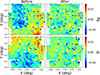 |
Fig. 2. Discretised calibration residuals before and after applying the FoV corrections determined by PhotCalib for the g and i filters. The first column shows the residuals for g (top) and i (bottom) before correction, and the second column shows the residuals after the correction is applied. |
As the FoV corrections are only dependent on filter and camera run, it was possible to use the CaHK corrections obtained by Pristine for camera run 22Am07 (Zhen Yuan, private communication). The CaHK corrections for our data were obtained by fitting the corrections from Pristine to the CaHK calibration residuals through χ2 minimisation. The majority of corrections are minor, |δCaHK|≤0.02; however, for a couple of GCs at the edges, the corrections reached values of δCaHK ∼ 0.04.
This leaves only the u magnitudes without FoV corrections. The scale of FoV corrections for u is expected to be similar to or slightly larger than that of the CaHK corrections (see Fig. 3 of Ibata et al. 2017).
The uncertainty on the photometry was initially calculated as the standard deviation from multiple measurements. Where only one measurement was available or the standard deviation was below the average statistical uncertainty, the average statistical uncertainty was adopted instead. Comparison with the calibration residuals showed that these calculated uncertainties were insufficient to explain the scatter of the residuals by a constant, the systematic uncertainty. The systematic uncertainty for each filter was determined through a maximum likelihood estimation under the assumption that the calibration residuals followed a Gaussian distribution with μi = 0 and σi2 = σsyn, i2 + (σphot, i + σsys)2, where σsyn, i and σphot, i are the uncertainty of the synthetic photometry and the calculated uncertainty for a calibration star and σsys is the to be fitted systematic uncertainty. This yielded: σsys, CaHK = 0.013, σsys, u = 0.023, σsys, g = 0.007, σsys, i = 0.006. For the majority of the GCs, this is the dominant contribution to their uncertainty.
Lastly, we estimated the uncertainty regarding background estimation by performing photometry with a different set of background estimation parameters that produced approximately the same background at larger scales. The average differences between the magnitudes were added to the uncertainties in quadrature, with only a small handful of GCs being significantly impacted. The magnitudes and final uncertainties can be found in Table B.1.
Figure 3 shows the comparison between our photometry and the published photometry of Peacock et al. (2010), which is the largest catalogue of ugriz photometry for M31 GCs. The Peacock et al. (2010) photometry is SDSS ugriz, which were transformed to MegaCam ugriz using the same transformations as used for calibration to enable comparison. These transformations are largely based on stars, so applying these to GCs can introduce more scatter or systematic errors. Additionally, the shown uncertainties do not include the uncertainty of the transformations, so it is expected that the scatter is larger than the plotted uncertainties. However, it can still be used to check for consistency between the sets of photometry.
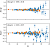 |
Fig. 3. Differences in u − g (top) and g − i (bottom) between our photometry and the Peacock et al. (2010) photometry converted to MegaCam colours. The text in the upper left of each plot is the average difference and scatter for the entire comparison sample. |
There is good consistency for u − g, but there is a 0.03 mag offset for g − i. Lacking correlations with GC structural parameters or the SDSS colours, the small offset is likely caused by the transformations and is not an actual offset in the photometry. There is, however, a group of outliers in g − i. Visual inspection of these GCs revealed that they lie in crowded or dense regions, mostly near the core of M31, making background estimation very difficult. This means that the outliers are caused by the different choices in background estimation. The offset of these outliers may be amplified by the transformations, so we believe that there is consistency between the sets of photometry.
3. Results
With the express goal of CaHK photometry being to measure the strength of the Ca II H & K lines, the combinations of CaHK with the u and g filters are of particular interest, as these filters directly flank CaHK on the shorter and longer wavelengths, respectively. This allows the u and g magnitudes to act as a measurement of the local continuum, which normalises the CaHK magnitude. Therefore, we investigated CaHK-u and CaHK-g.
Figure 4 shows each of the CaHK colours as a function of metallicity for the GC sample. Despite earlier concerns with regards to the quality of the reddening estimates, the similarity seen between GCs with and without robust reddening estimates shows that this is not an issue at the scale of the colours.
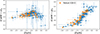 |
Fig. 4. (CaHK-u)o (left) and (CaHK-g)o (right) vs metallicity for the GC sample. The GCs with robust reddening estimates are shown as orange diamonds, and the others as blue circles. EXT8 can be seen separating itself from the other metal-poor GCs as the leftmost GC in each plot. Note the difference in vertical scale between the two panels (0.1 vs 0.2 mag major tick spacing). |
In the left plot of Fig. 4, it can be seen that the values of CaHK-u remain within a small range, Δ(CaHK − u)∼0.2, across the entire metallicity range. The relation appears to be non-monotonic when considering GCs with [Fe/H] ≥ −0.8 separately from GCs with [Fe/H] ≤ −0.8. (CaHK − u)o is negatively correlated with metallicity for [Fe/H] ≥ −0.8, with (CaHK − u)o decreasing in value from ∼0.4 at [Fe/H] = −0.8 to ∼0.27 at [Fe/H] = 0, with a suggestion of even lower values for super-solar metallicities. A Spearman correlation test gives a correlation coefficient of ![Mathematical equation: $ \rho_{\text{[Fe/H]} \geq -0.8} = -0.67^{+0.18}_{-0.13} $](/articles/aa/full_html/2025/11/aa55441-25/aa55441-25-eq2.gif) , where the uncertainty is the 95 percent confidence interval. For [Fe/H] ≤ −0.8, (CaHK − u)o shows a positive correlation as its value decreases from ∼0.4 back to a similar value of the solar metallicity GCs for the most metal-poor GCs as the metallicity decreases with
, where the uncertainty is the 95 percent confidence interval. For [Fe/H] ≤ −0.8, (CaHK − u)o shows a positive correlation as its value decreases from ∼0.4 back to a similar value of the solar metallicity GCs for the most metal-poor GCs as the metallicity decreases with ![Mathematical equation: $ \rho_{\text{[Fe/H]} \leq -0.8} = 0.52^{+0.18}_{-0.14} $](/articles/aa/full_html/2025/11/aa55441-25/aa55441-25-eq3.gif) . The non-monotonic relation with metallicity makes the interpretation of (CaHK − u)o as a measure of CaHK strength difficult as a single (CaHK − u)0 value can correspond to two, potentially drastically different, metallicities. Therefore, (CaHK − u)o must always be used in conjunction with another colour that can break the degeneracy.
. The non-monotonic relation with metallicity makes the interpretation of (CaHK − u)o as a measure of CaHK strength difficult as a single (CaHK − u)0 value can correspond to two, potentially drastically different, metallicities. Therefore, (CaHK − u)o must always be used in conjunction with another colour that can break the degeneracy.
In the right plot of Fig. 4, (CaHK − g)o shows a strong positive correlation with metallicity ( ), changing by about 0.8 magnitudes across the entire metallicity range, from ∼1.3 at solar metallicity down to ∼0.5 at the very metal-poor end. (CaHK − g)o seems to experience a break around [Fe/H] = −1.4, as the slope of the relation noticeably decreases. For [Fe/H] ≤ −1.4, the correlation coefficient decreases to
 ![Mathematical equation: $ \rho_{\text{[Fe/H]} \leq -1.4} = 0.60^{+0.18}_{-0.28} $](/articles/aa/full_html/2025/11/aa55441-25/aa55441-25-eq5.gif) while for [Fe/H] ≥ −1.4 the correlation coefficient remains relatively similar:
while for [Fe/H] ≥ −1.4 the correlation coefficient remains relatively similar: ![Mathematical equation: $ \rho_{\text{[Fe/H]} \geq -1.4} = 0.89^{+0.03}_{-0.05} $](/articles/aa/full_html/2025/11/aa55441-25/aa55441-25-eq6.gif) . The relation shown by (CaHK − g)o is reminiscent of the bilinear relation commonly found for metallicity sensitive spectral indices for GCs (e.g. Burstein et al. 1984). This suggests that (CaHK − g)o provides a simple measurement of the strength of the Ca II H & K lines and makes the interpretation of (CaHK − g)o straightforward, with low (CaHK − g)o values corresponding with weak Ca II H & K lines, and vice versa.
. The relation shown by (CaHK − g)o is reminiscent of the bilinear relation commonly found for metallicity sensitive spectral indices for GCs (e.g. Burstein et al. 1984). This suggests that (CaHK − g)o provides a simple measurement of the strength of the Ca II H & K lines and makes the interpretation of (CaHK − g)o straightforward, with low (CaHK − g)o values corresponding with weak Ca II H & K lines, and vice versa.
For our purpose, the interest lies in the metal-poor regime ([Fe/H] ≤ −1.5), with the main question being whether EXT8 can be separated from regular metal-poor GCs. EXT8, as the most metal-poor GC in the sample, can be easily identified as the leftmost GC in each of the plots in Fig. 4 as an orange diamond. In (CaHK − g)o, EXT8 clearly stands out from the other metal-poor GCs as it has the lowest (CaHK − g)o value, (CaHK − g)o = 0.49 ± 0.02, by which it is separated from the closest regular metal-poor GCs by 0.07. In (CaHK − u)o, EXT8 does not separate itself as clearly from the other metal-poor GCs as its (CaHK − u)o value, (CaHK − u)o = 0.28 ± 0.04, is only separated by 0.004 from the nearest regular metal-poor GC.
Alongside EXT8, the two potential GCs below the metallicity floor in the sample, B160-G214 ([Fe/H] = −2.8 ± 0.4) and B157-G212 ([Fe/H] = −2.6 ± 0.3), show similar behaviour as EXT8. In (CaHK − g)o, they separate themselves from the more metal-rich GCs but show a slightly higher (CaHK − g)o than EXT8, hinting at a good metallicity sensitivity of (CaHK − g)o even near the extremely metal-poor regime. In (CaHK − u)o, they show equivalent values to EXT8 within their uncertainty with B160-G214 showing a slightly lower value.
Considering all metal-poor GCs ([Fe/H] ≤ −1.5) suggests that the behaviour of both CaHK colours in the metal-poor regime is linear, although the sparse amount of GCs in this regime makes it difficult to infer anything but linear behaviour. Regardless, fitting a linear relation to the metal-poor GCs through unweighted least-squares gives the following relations:
![Mathematical equation: $$ \begin{aligned} (CaHK-u)_{o}&= (0.064\pm 0.012)\text{[Fe/H]} + (0.456\pm 0.023)\nonumber \\ (CaHK-g)_{o}&= (0.177\pm 0.032)\text{[Fe/H]} + (0.994\pm 0.062). \end{aligned} $$](/articles/aa/full_html/2025/11/aa55441-25/aa55441-25-eq7.gif) (1)
(1)
The RMS of the fits are 0.02 mag and 0.06 mag for (CaHK − u)o and (CaHK − g)o, respectively. Despite the substantial difference in slope, for both (CaHK − u)o and (CaHK − g)o the uncertainty on metallicity estimates suggested by the RMS would be 0.3 dex at a 1σ level.
3.1. Comparison with other GC colours
EXT8 and the other potential GCs below the metallicity floor have shown that CaHK photometry holds up to its suggested potential for candidate selection, with (CaHK − g)o providing a clean selection of these GCs, but how do the CaHK colours compare to potential alternative GC colours that could be considered for the same purpose?
One might consider using u − g, as the u filter covers the metallicity-sensitive shorter wavelengths and requires a lower integration time to reach similar S/N due to its broadband nature compared to CaHK. From literature, the g-z colour from SDSS filters, or equivalently F450W-F850L from HST filters, has seen significant usage in studying extragalactic GC systems alongside spectroscopic campaigns (e.g. Peng et al. 2006; Sinnott et al. 2010; Usher et al. 2012; Villaume et al. 2019; Fahrion et al. 2020). This makes g-z an appealing option, as it is more readily available and has been spectroscopically calibrated.
Figure 5 shows (u − g)o in the top panel and (g − z)SDSS, o from Peacock et al. (2010) in the lower panel. The lower panel with (g − z)SDSS, o also shows the spectroscopically determined colour-metallicity relations (CMRs) from Peng et al. (2006), Sinnott et al. (2010), and Usher et al. (2012). The extinction coefficients for SDSS g and z filters were approximated in the same way as for the MegaCam filters, yielding cg, SDSS = 3.751 and cz, SDSS = 1.587.
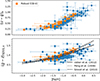 |
Fig. 5. Broadband colours, (u − g)o (top) and (g − z)SDSS, o (bottom), plotted against metallicity for our GC sample. For (g − z)SDSS, o, the spectroscopically calibrated CMRs from Peng et al. (2006, dotted), Sinnott et al. (2010, dashed), and Usher et al. (2012, solid) are also plotted. For both colours, the GCs below the metallicity do not separate clearly from other GCs. |
From Fig. 5, it can be seen that the GCs below the metallicity floor do not separate as well in both colours as they do in (CaHK − g)o. In the GC sample the colour values of the GCs below the metallicity floor can also be found for GCs up to [Fe/H] = −2 for (u − g)o and for (g − z)SDSS, o all the way up to [Fe/H] = −0.6. For (g − z)SDSS, o. The majority of these GCs have more uncertain reddening estimate, but even for the GCs with the more robust reddening EXT8 has a similar (g − z)SDSS, o value to GCs up to [Fe/H] = −1.3.
All three spectroscopically calibrated CMRs for (g − z)SDSS, o fit reasonably well to the data and predict the blue colour of B157 and B160 within their uncertainty. EXT8 is, however, slightly redder and would be missed when utilising any of the three CMRs. This suggests that the metallicity sensitivity of (g − z)SDSS, o is lower than predicted by extrapolation of the literature CMRs.
Performing the same linear fits for (u − g)o and (g − z)SDSS, o as for the CaHK colours yields the following relations:
![Mathematical equation: $$ \begin{aligned} (u-g)_{o}&= (0.111\pm 0.029)\text{[Fe/H]} + (0.535\pm 0.056)\nonumber \\ (g-z)_{\mathrm{SDSS} ,o}&= (0.118\pm 0.047)\text{[Fe/H]} + (1.022\pm 0.090). \end{aligned} $$](/articles/aa/full_html/2025/11/aa55441-25/aa55441-25-eq8.gif) (2)
(2)
The RMS of the fits are 0.05 mag and 0.08 mag for (u − g)o and (g − z)SDSS, o, respectively. The RMS of the fits suggest an uncertainty of 0.5 dex and 0.7 dex on metallicity estimates using (u − g)o and (g − z)SDSS, o. Both of these are worse than the metallicity uncertainty of the CaHK colours.
The literature (g − z)SDSS, o CMRs report uncertainties on metallicity estimates between 0.17 and 0.3 dex, which would make them better or on par with the CaHK colours. The difference between the reported uncertainties and those found here has to do with the different GCs, data and the metallicity range over which was fitted. The high uncertainty on reddening estimates can play a significant role for (g − z)SDSS, o; however, the GCs with more robust reddening estimates show a similar RMS.
The lower uncertainty on metallicity estimations mean that the CaHK colours provide a less contaminated selection compared to (u − g)o and (g − z)SDSS, o. Using the GC metallicity distributions of the Galaxy (Harris 1996, 2010 edition) and M31 (C&R16) with the fit RMS as a Gaussian scatter on the CMRs, the CaHK colours have a false positive identification rate around 4 percent for GCs with −2.5 ≤ [Fe/H] ≤ −1.5 to be identified as a GC with [Fe/H] ≤ −2.5. This is a factor of 2 better than (u − g)o and a factor of 3.8 better than (g − z)SDSS, o. The high-S/N and high-resolution of Larsen et al. (2020) for EXT8, a relatively close by and bright GC, already had an integration time of 40 minutes. This means that reducing the selection contamination by a factor of 2 is a significant reduction in telescope time for future spectroscopic observations. This is especially true for more distant systems and massive galaxies that can host several hundreds up to thousands of GCs with [Fe/H] ≤ −1.5 (e.g. Harris 2023).
A principal component analysis test was done with the available colours to see if any colour combination would perform better than the CaHK colours alone. The best principal component analysis component, predominantly relying on (CaHK − g)o and (u − g)o, showed an uncertainty on metallicity estimation of 0.4 dex, slightly worse than the individual CaHK colours.
3.2. Horizontal branch morphology sensitivity
Metallicity is one of the main parameters that determines horizontal branch (HB) morphology, with metal-rich GCs showing cooler red HB populations while metal-poor GCs show hotter blue HB populations (e.g. Arp et al. 1952). The Galactic GCs (GGCs) at similar metallicity, however, show a wider range of morphologies with some showing both a red and a blue HB or an extended HB with a characteristic tail. This phenomenon is known as the ‘second parameter’ problem (e.g. van den Bergh 1965; Gratton et al. 2010; Dotter et al. 2010).
The differences in HB morphology have been tied to other GC properties. The main culprits are GC age and helium variations within a GC (e.g. Sandage & Wildey 1967; Searle & Zinn 1978; Lee et al. 1994; Milone et al. 2014). A younger age causes the HB to be redder at the same metallicity, and larger helium variations cause a more extended HB. The latter is tied to the multiple population phenomenon, which can additionally explain the existence of bimodal HB morphologies (e.g. Marino et al. 2011).
It is well known that the HB morphology significantly influences the colours and line indices of GCs, especially the Balmer lines (e.g. Lee et al. 2000, 2002; Schiavon et al. 2004; Percival & Salaris 2011). The CaHK colours are likely not an exception to this, as the Ca II H & K lines are located in the UV and Ca II H is blended with the Hϵ Balmer line. If the CaHK colours are sufficiently sensitive to HB morphology, it can cause complications for candidate selection. An example would be if an intermediate metallicity GC with a very blue HB morphology mimics the CaHK colours of a GC at or below the metallicity floor.
There are only a small number of HB morphology measurements for GCs in our sample, 8 measurements from Perina et al. (2012) and one for EXT8 from Larsen et al. (2021). Perina et al. (2012) measured the HB morphology with the simplified Mironov index (SMI)  , where B and R are the number of HB stars bluer or redder than a given colour threshold, usually chosen in the middle of the RR Lyrae instability strip. Small SMI values indicate a red dominant branch while large SMI values indicate a blue dominant branch. All but one (B407-G352; SMI = 0 ± 0.1) of the SMI values from Perina et al. (2012) for our sample were derived from lower-quality CMDs and are considered to be lower limits, as blue HB stars could fall below the limiting magnitude of the CMDs.
Figure 6 shows the HB morphologies for the nine M31 GCs alongside that of the GGCs. B158-G223 (square) has a substantially higher SMI (0.63 ± 0.37) for its metallicity, suggesting the presence of an unusually large blue HB component. The set of B220-G275, B224-G279, and B240-G302 (pluses) show redder branches (SMI = 0.39 ± 0.2, 0.43 ± 0.19, and 0.63 ± 0.37), similar to M3 among the GGCs (e.g. Rey et al. 2001), meaning these GCs are younger.
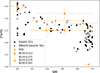 |
Fig. 6. SMI vs metallicity diagram. The nine M31 GCs are plotted in orange. The GGCs are plotted as black circles. The SMI for the GGCs is a combination of data from Perina et al. (2012) and Lee et al. (1994). The Lee et al. (1994) HB ratio values were converted to SMI using the Preston et al. (1991) relation. The GGC metallicities were taken from Harris (1996, 2010 edition) The GGCs that have WAGGS spectra (Usher et al. 2017) are shown as open black circles. |
Figure 7 shows the CaHK CMRs with the SMI values of the 9 GCs plotted overtop as a colour alongside the median trend for the CMRs. Only B158-G223 in (CaHK − u)o seems to strongly deviate from the median trend by 0.07 mag. B158-G223 does, however, lie at the edge of the inner field covering the disc of M31. This suggests that it is subject to a large FoV correction for its u magnitude, which would shift its (CaHK − u)o value towards the median.
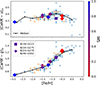 |
Fig. 7. CaHK CMRs of Fig. 4 overlaid with the HB morphology measurements from Perina et al. (2012) and Larsen et al. (2021) in colour. Red corresponds to a red branch and blue to a blue branch. The black line shows the median trend for each of the CaHK colours, calculated with a binwidth of 0.4 dex. Note the difference in vertical scale between the two panels (0.1 vs 0.2 mag major tick spacing). |
In addition to the nine M31 GCs, we investigated the GGCs by generating synthetic colours from the spectra of the WiFeS Atlas of Galatic Globular cluster Spectra (WAGGS) (Usher et al. 2017). The WAGGS spectra are a set of relatively calibrated spectra covering 62 GGCs (marked by open circles in Fig. 6) from 3270 Å to 9050 Å.
Similar to the M31 GCs, we find that differing HB morphologies at the same metallicity do not strongly affect the CaHK colours. It should be kept in mind that the WAGGS spectra, like other integrated-light spectra, only capture a fraction of the total cluster light (the median fraction of V-band light is 0.12; Usher et al. 2017) making them susceptible to stochastic variations and repeat observations showed that the UV wavelengths of the spectra have variations up to 12 percent.
In the end, we do not find any indication of a strong HB morphology sensitivity, meaning that differing morphologies are unlikely to present an issue for candidate selection. However, neither of the datasets contained metal-poor, red HB GCs ([Fe/H] ≤ −1.5 and SMI ≤ 0.2), of which more extreme versions of the GGCs were recently discovered in the outer halo of M31 (McGill et al. 2025). Ultimately, this assessment is limited by the amount and quality of the available data and should be followed up with a more in-depth assessment with more robust data.
4. Conclusion
In order to lay the groundwork for a more organised search for other GCs similar to EXT8, we investigated the behaviour of the CaHK colours, CaHK-u and CaHK-g, with metallicity for the purpose of candidate selection with a sample of M31 GCs, including EXT8.
(CaHK − u)o shows a non-monotonic CMR with a maximum around [Fe/H] = −0.8, which results in a small colour range; it must be used in conjunction with another colour to break the degeneracy. (CaHK − g)o shows an approximately bilinear CMR, similar to that of metallicity-sensitive spectral indices, suggesting that (CaHK − g)o is a straightforward measurement of the Ca II H & K lines. Despite significant differences in metallicity sensitivity in the metal-poor regime, with (CaHK − g)o showing 0.177 ± 0.032 mag/dex, the RMS values of the relations for both CaHK colours suggest an uncertainty of 0.3 dex on metallicity estimates from the colours. In comparison with the broadband colours (u − g)o and (g − z)SDSS, o, the CaHK colours could reduce false positive identification rates and by extension the follow-up observation time by at least a factor of 2. We also investigated the influence of the HB morphology based on available data and found no indication that HB morphology affects the CaHK colours to a degree that would pose a problem for candidate selection.
The results presented here are an initial test for CaHK photometry for GCs and far from conclusive, given the unavoidable sparseness of GCs in the metal-poor regime, limited robust information of M31 GC properties in our sample, and potential differences between GC systems (e.g. Usher et al. 2015; Powalka et al. 2016). Despite these limitations, we find that CaHK photometry for GCs does hold up to its suggested potential and can be used as an effective indicator of metallicity in order to identify candidates for massive GCs below the metallicity floor.
While (CaHK − g)o can in principle be used alone for candidate selection, using it in conjunction with other colours naturally provides more information for candidate selection. Primarily, the inclusion of u-based colours would fully characterise the wavelength region around the Ca II H & K lines. The fitted relations for all colours presented in this study suggest that GCs below the metallicity floor should have the following colour values: (CaHK − g)o ≤ 0.551, (CaHK − u)o ≤ 0.295, (u − g)o ≤ 0.258, and (g − z)SDSS, o ≤ 0.727.
This study marks the beginning of the search for massive GCs below the metallicity floor carried out in order to learn if and/or how this previously unknown class of GC fits into our understanding of GC formation. With the expectation that, in general, GCs below the metallicity floor must originate from dwarf galaxies, the haloes of massive galaxies make for a good starting point as these haloes have accreted a substantial amount of dwarf systems.
The best estimates of the rarity of EXT8-like GCs are 0.05 percent (empirical; Beasley et al. 2019) and 0.03 percent (simulation; Usher et al. 2018), which means that even in massive haloes that can hold up to several thousand GCs (e.g. Durrell et al. 2014; Harris 2023), only a handful of EXT8-like GCs are expected. This means the effectiveness of the CaHK colours will be key for the search effort.
Acknowledgments
Based on observations obtained with MegaPrime/MegaCam, a joint project of CFHT and CEA/DAPNIA, at the Canada-France-Hawaii Telescope (CFHT) which is operated by the National Research Council (NRC) of Canada, the Institut National des Science de l’Univers of the Centre National de la Recherche Scientifique (CNRS) of France, and the University of Hawaii. The observations at the Canada-France-Hawaii Telescope were performed with care and respect from the summit of Maunakea which is a significant cultural and historic site. The authors thank the referee for their comments and suggestions that helped improve the quality of this manuscript. BvH is grateful to Zhen Yuan and Nicolas Martin for kindly sharing the CaHK FoV correction for camera run 22Am07. ES warmly acknowledges helpful discussions with Eric Peng on this subject. WEH acknowledges support from the Natural Sciences and Engineering Research Council of Canada. ES acknowledges funding through VIDI grant “Pushing Galactic Archeology to its limits” (with project number VI. Vidi.193.093) which is funded by the Dutch Research Council (NWO). This research has been partially funded from a Spinoza award by NWO (SPI 78-411). This work has made use of NUMPY (van der Walt et al. 2011), MATPLOTLIB (Hunter 2007) and SCIPY (Virtanen et al. 2020).
References
- Abel, T., Bryan, G. L., & Norman, M. L. 2002, Science, 295, 93 [CrossRef] [Google Scholar]
- Arp, H. C., Baum, W. A., & Sandage, A. R. 1952, AJ, 57, 4 [CrossRef] [Google Scholar]
- Barmby, P., Huchra, J. P., Brodie, J. P., et al. 2000, AJ, 119, 727 [NASA ADS] [CrossRef] [Google Scholar]
- Beasley, M. A., Leaman, R., Gallart, C., et al. 2019, MNRAS, 487, 1986 [Google Scholar]
- Beers, T. C., Preston, G. W., & Shectman, S. A. 1992, AJ, 103, 1987 [NASA ADS] [CrossRef] [Google Scholar]
- Bertin, E., & Arnouts, S. 1996, A&AS, 117, 393 [NASA ADS] [CrossRef] [EDP Sciences] [Google Scholar]
- Bond, H. E. 1981, ApJ, 248, 606 [NASA ADS] [CrossRef] [Google Scholar]
- Burstein, D., Faber, S. M., Gaskell, C. M., & Krumm, N. 1984, ApJ, 287, 586 [Google Scholar]
- Caldwell, N., & Romanowsky, A. J. 2016, ApJ, 824, 42 [NASA ADS] [CrossRef] [Google Scholar]
- Caldwell, N., Schiavon, R., Morrison, H., Rose, J. A., & Harding, P. 2011, AJ, 141, 61 [NASA ADS] [CrossRef] [Google Scholar]
- Carlberg, R. G., Ibata, R., Martin, N. F., et al. 2025, ApJ, 988, 96 [Google Scholar]
- Carney, B. W., Laird, J. B., Latham, D. W., & Aguilar, L. A. 1996, AJ, 112, 668 [NASA ADS] [CrossRef] [Google Scholar]
- Christlieb, N., Schörck, T., Frebel, A., et al. 2008, A&A, 484, 721 [NASA ADS] [CrossRef] [EDP Sciences] [Google Scholar]
- Dotter, A., Sarajedini, A., Anderson, J., et al. 2010, ApJ, 708, 698 [Google Scholar]
- Durrell, P. R., Cĉté, P., Peng, E. W., et al. 2014, ApJ, 794, 103 [NASA ADS] [CrossRef] [Google Scholar]
- Errani, R., Navarro, J. F., Ibata, R., et al. 2022, MNRAS, 514, 3532 [NASA ADS] [CrossRef] [Google Scholar]
- Fahrion, K., Lyubenova, M., Hilker, M., et al. 2020, A&A, 637, A27 [NASA ADS] [CrossRef] [EDP Sciences] [Google Scholar]
- Fan, Z., de Grijs, R., & Zhou, X. 2010, ApJ, 725, 200 [Google Scholar]
- Federici, L., Cacciari, C., Bellazzini, M., et al. 2012, A&A, 544, A155 [NASA ADS] [CrossRef] [EDP Sciences] [Google Scholar]
- Fitzpatrick, E. L. 1999, PASP, 111, 63 [Google Scholar]
- Forbes, D. A., Bastian, N., Gieles, M., et al. 2018, Proc. R. Soc. London Ser. A, 474, 20170616 [Google Scholar]
- Gaia Collaboration (Montegriffo, P., et al.) 2023, A&A, 674, A33 [CrossRef] [EDP Sciences] [Google Scholar]
- Gratton, R. G., Carretta, E., Bragaglia, A., Lucatello, S., & D’Orazi, V. 2010, A&A, 517, A81 [CrossRef] [EDP Sciences] [Google Scholar]
- Harris, W. E. 1996, AJ, 112, 1487 [Google Scholar]
- Harris, W. E. 2023, ApJS, 265, 9 [CrossRef] [Google Scholar]
- Hunter, J. D. 2007, Comput. Sci. Eng., 9, 90 [NASA ADS] [CrossRef] [Google Scholar]
- Ibata, R. A., McConnachie, A., Cuillandre, J.-C., et al. 2017, ApJ, 848, 128 [Google Scholar]
- Kang, Y., Rey, S.-C., Bianchi, L., et al. 2012, ApJS, 199, 37 [Google Scholar]
- Keller, S. C., Schmidt, B. P., & Bessell, M. S. 2008, in 2007 ESO Instrument Calibration Workshop, eds. A. Kaufer, & F. Kerber, 573 [Google Scholar]
- Kruijssen, J. M. D. 2015, MNRAS, 454, 1658 [Google Scholar]
- Kruijssen, J. M. D. 2019, MNRAS, 486, L20 [NASA ADS] [CrossRef] [Google Scholar]
- Larsen, S. S., Romanowsky, A. J., Brodie, J. P., & Wasserman, A. 2020, Science, 370, 970 [NASA ADS] [CrossRef] [Google Scholar]
- Larsen, S. S., Romanowsky, A. J., & Brodie, J. P. 2021, A&A, 651, A102 [NASA ADS] [CrossRef] [EDP Sciences] [Google Scholar]
- Lee, Y.-W., Demarque, P., & Zinn, R. 1994, ApJ, 423, 248 [NASA ADS] [CrossRef] [Google Scholar]
- Lee, H.-C., Yoon, S.-J., & Lee, Y.-W. 2000, AJ, 120, 998 [NASA ADS] [Google Scholar]
- Lee, H.-C., Lee, Y.-W., & Gibson, B. K. 2002, AJ, 124, 2664 [CrossRef] [Google Scholar]
- Lindegren, L., Klioner, S. A., Hernández, J., et al. 2021, A&A, 649, A2 [EDP Sciences] [Google Scholar]
- Loeb, A., & Rasio, F. A. 1994, ApJ, 432, 52 [Google Scholar]
- Magnier, E. A., & Cuillandre, J. C. 2004, PASP, 116, 449 [NASA ADS] [CrossRef] [Google Scholar]
- Marino, A. F., Villanova, S., Milone, A. P., et al. 2011, ApJ, 730, L16 [NASA ADS] [CrossRef] [Google Scholar]
- Martin, N. F., Venn, K. A., Aguado, D. S., et al. 2022, Nature, 601, 45 [NASA ADS] [CrossRef] [Google Scholar]
- Martin, N. F., Starkenburg, E., Yuan, Z., et al. 2024, A&A, 692, A115 [NASA ADS] [CrossRef] [EDP Sciences] [Google Scholar]
- McGill, G., Ferguson, A. M. N., Mackey, D., et al. 2025, MNRAS, 542, L60 [Google Scholar]
- Milone, A. P., Marino, A. F., Dotter, A., et al. 2014, ApJ, 785, 21 [NASA ADS] [CrossRef] [Google Scholar]
- Peacock, M. B., Maccarone, T. J., Knigge, C., et al. 2010, MNRAS, 402, 803 [NASA ADS] [CrossRef] [Google Scholar]
- Peng, E. W., Jordán, A., Cĉté, P., et al. 2006, ApJ, 639, 95 [Google Scholar]
- Percival, S. M., & Salaris, M. 2011, MNRAS, 412, 2445 [CrossRef] [Google Scholar]
- Perina, S., Bellazzini, M., Buzzoni, A., et al. 2012, A&A, 546, A31 [NASA ADS] [CrossRef] [EDP Sciences] [Google Scholar]
- Powalka, M., Puzia, T. H., Lançon, A., et al. 2016, ApJ, 829, L5 [NASA ADS] [CrossRef] [Google Scholar]
- Preston, G. W., Shectman, S. A., & Beers, T. C. 1991, ApJ, 375, 121 [Google Scholar]
- Regnault, N., Conley, A., Guy, J., et al. 2009, A&A, 506, 999 [NASA ADS] [CrossRef] [EDP Sciences] [Google Scholar]
- Reina-Campos, M., Kruijssen, J. M. D., Pfeffer, J., Bastian, N., & Crain, R. A. 2018, MNRAS, 481, 2851 [NASA ADS] [CrossRef] [Google Scholar]
- Rey, S.-C., Yoon, S.-J., Lee, Y.-W., Chaboyer, B., & Sarajedini, A. 2001, AJ, 122, 3219 [Google Scholar]
- Riello, M., De Angeli, F., Evans, D. W., et al. 2021, A&A, 649, A3 [NASA ADS] [CrossRef] [EDP Sciences] [Google Scholar]
- Sandage, A., & Wildey, R. 1967, ApJ, 150, 469 [NASA ADS] [CrossRef] [Google Scholar]
- Schiavon, R. P., Rose, J. A., Courteau, S., & MacArthur, L. A. 2004, ApJ, 608, L33 [NASA ADS] [CrossRef] [Google Scholar]
- Schlafly, E. F., & Finkbeiner, D. P. 2011, ApJ, 737, 103 [Google Scholar]
- Schlafly, E. F., Finkbeiner, D. P., Schlegel, D. J., et al. 2010, ApJ, 725, 1175 [NASA ADS] [CrossRef] [Google Scholar]
- Schlegel, D. J., Finkbeiner, D. P., & Davis, M. 1998, ApJ, 500, 525 [Google Scholar]
- Searle, L., & Zinn, R. 1978, ApJ, 225, 357 [Google Scholar]
- Sinnott, B., Hou, A., Anderson, R., Harris, W. E., & Woodley, K. A. 2010, AJ, 140, 2101 [Google Scholar]
- Starkenburg, E., Martin, N., Youakim, K., et al. 2017, MNRAS, 471, 2587 [NASA ADS] [CrossRef] [Google Scholar]
- Usher, C., Forbes, D. A., Brodie, J. P., et al. 2012, MNRAS, 426, 1475 [Google Scholar]
- Usher, C., Forbes, D. A., Brodie, J. P., et al. 2015, MNRAS, 446, 369 [NASA ADS] [CrossRef] [Google Scholar]
- Usher, C., Pastorello, N., Bellstedt, S., et al. 2017, MNRAS, 468, 3828 [NASA ADS] [CrossRef] [Google Scholar]
- Usher, C., Pfeffer, J., Bastian, N., et al. 2018, MNRAS, 480, 3279 [NASA ADS] [CrossRef] [Google Scholar]
- van den Bergh, S. 1962, AJ, 67, 486 [Google Scholar]
- van den Bergh, S. 1965, JRASC, 59, 151 [NASA ADS] [Google Scholar]
- van der Walt, S., Colbert, S. C., & Varoquaux, G. 2011, Comput. Sci. Eng., 13, 22 [Google Scholar]
- Villaume, A., Romanowsky, A. J., Brodie, J., & Strader, J. 2019, ApJ, 879, 45 [NASA ADS] [CrossRef] [Google Scholar]
- Virtanen, P., Gommers, R., Oliphant, T. E., et al. 2020, Nat. Methods, 17, 261 [Google Scholar]
- Viswanathan, A., Yuan, Z., Ardern-Arentsen, A., et al. 2025, A&A, 695, A112 [NASA ADS] [CrossRef] [EDP Sciences] [Google Scholar]
- Wan, Z., Lewis, G. F., Li, T. S., et al. 2020, Nature, 583, 768 [Google Scholar]
- Youakim, K., Starkenburg, E., Martin, N. F., et al. 2020, MNRAS, 492, 4986 [CrossRef] [Google Scholar]
- Yuan, Z., Martin, N. F., Ibata, R. A., et al. 2022, MNRAS, 514, 1664 [CrossRef] [Google Scholar]
- Yuan, Z., Matsuno, T., Sitnova, T. M., et al. 2025, A&A, 698, A82 [NASA ADS] [CrossRef] [EDP Sciences] [Google Scholar]
- Zinn, R. 1980, ApJS, 42, 19 [Google Scholar]
Appendix A: Observing logs
Observing logs for each of the fields and the main parameters for each exposure obtained.
Appendix B: Globular cluster parameters and photometry
Metallicity, aperture photometry results, and reddening for the sample of M31 GCs.
All Tables
Observing logs for each of the fields and the main parameters for each exposure obtained.
Metallicity, aperture photometry results, and reddening for the sample of M31 GCs.
All Figures
|
Fig. 1. Observational footprint of this study. The GC sample is marked with either orange diamonds or blue circles, signifying GCs with and without robust reddening estimates. EXT8 is marked in red, and the black circles are confirmed M31 GCs from the C&R16 catalogue that were not considered. The background colour is the reddening from the Schlegel et al. (1998) dust map with the correction of Schlafly et al. (2010), clearly highlighting M31 itself. The two rectangles with ‘ears’ are the observed fields that form the footprint for this study. |
| In the text | |
|
Fig. 2. Discretised calibration residuals before and after applying the FoV corrections determined by PhotCalib for the g and i filters. The first column shows the residuals for g (top) and i (bottom) before correction, and the second column shows the residuals after the correction is applied. |
| In the text | |
|
Fig. 3. Differences in u − g (top) and g − i (bottom) between our photometry and the Peacock et al. (2010) photometry converted to MegaCam colours. The text in the upper left of each plot is the average difference and scatter for the entire comparison sample. |
| In the text | |
|
Fig. 4. (CaHK-u)o (left) and (CaHK-g)o (right) vs metallicity for the GC sample. The GCs with robust reddening estimates are shown as orange diamonds, and the others as blue circles. EXT8 can be seen separating itself from the other metal-poor GCs as the leftmost GC in each plot. Note the difference in vertical scale between the two panels (0.1 vs 0.2 mag major tick spacing). |
| In the text | |
|
Fig. 5. Broadband colours, (u − g)o (top) and (g − z)SDSS, o (bottom), plotted against metallicity for our GC sample. For (g − z)SDSS, o, the spectroscopically calibrated CMRs from Peng et al. (2006, dotted), Sinnott et al. (2010, dashed), and Usher et al. (2012, solid) are also plotted. For both colours, the GCs below the metallicity do not separate clearly from other GCs. |
| In the text | |
|
Fig. 6. SMI vs metallicity diagram. The nine M31 GCs are plotted in orange. The GGCs are plotted as black circles. The SMI for the GGCs is a combination of data from Perina et al. (2012) and Lee et al. (1994). The Lee et al. (1994) HB ratio values were converted to SMI using the Preston et al. (1991) relation. The GGC metallicities were taken from Harris (1996, 2010 edition) The GGCs that have WAGGS spectra (Usher et al. 2017) are shown as open black circles. |
| In the text | |
|
Fig. 7. CaHK CMRs of Fig. 4 overlaid with the HB morphology measurements from Perina et al. (2012) and Larsen et al. (2021) in colour. Red corresponds to a red branch and blue to a blue branch. The black line shows the median trend for each of the CaHK colours, calculated with a binwidth of 0.4 dex. Note the difference in vertical scale between the two panels (0.1 vs 0.2 mag major tick spacing). |
| In the text | |
Current usage metrics show cumulative count of Article Views (full-text article views including HTML views, PDF and ePub downloads, according to the available data) and Abstracts Views on Vision4Press platform.
Data correspond to usage on the plateform after 2015. The current usage metrics is available 48-96 hours after online publication and is updated daily on week days.
Initial download of the metrics may take a while.