| Issue |
A&A
Volume 703, November 2025
|
|
|---|---|---|
| Article Number | A171 | |
| Number of page(s) | 16 | |
| Section | Stellar structure and evolution | |
| DOI | https://doi.org/10.1051/0004-6361/202555734 | |
| Published online | 21 November 2025 | |
The 2025 outburst of IGR J17511−3057: Timing and spectral insights from NICER and NuSTAR
1
Dipartimento di Fisica, Università degli Studi di Cagliari, SP Monserrato-Sestu, KM 0.7, Monserrato 09042, Italy
2
DTU Space, Technical University of Denmark, Elektrovej 327-328, DK-2800 Lyngby, Denmark
3
Astrophysics Science Division and Joint Space-Science Institute, NASA’s Goddard Space Flight Center, Greenbelt, MD 20771, USA
4
INAF–Osservatorio Astronomico di Brera, Via Bianchi 46, I-23807 Merate (LC), Italy
5
INAF Osservatorio Astronomico di Roma, Via Frascati 33, 00078 Monte Porzio Catone (RM), Italy
6
Dipartimento di Fisica e Chimica – Emilio Segrè, Università di Palermo, Via Archirafi 36 – 90123, Palermo, Italy
7
INAF/IASF Palermo, Via Ugo La Malfa 153, I-90146 Palermo, Italy
8
Department of Physics and Astronomy, Howard University, Washington, DC 20059, USA
9
CRESST and NASA Goddard Space Flight Center, Astrophysics Science Division, 8800 Greenbelt Road, Greenbelt, MD, USA
10
School of Physics and Astronomy, University of Southampton, Southampton SO17 1BJ, UK
11
Department of Physics, McGill University, 3600 rue University, Montréal QC H3A 2T8, Canada
12
Trottier Space Institute at McGill University, 3550 rue University, Montréal QC H3A 2A7, Canada
13
MIT Kavli Institute for Astrophysics and Space Research, Massachusetts Institute of Technology, Cambridge, MA 02139, USA
14
Istanbul University, Graduate School of Sciences, Department of Astronomy and Space Sciences, Beyazıt, 34119 İstanbul, Türkiye
⋆ Corresponding author: This email address is being protected from spambots. You need JavaScript enabled to view it.
Received:
30
May
2025
Accepted:
18
September
2025
Abstract
Context. IGR J17511−3057 is an accreting millisecond X-ray pulsar and a known type-I burster. The source was observed in outburst for the first time in 2009 and again in 2015, followed by a decade-long quiescence phase.
Aims. The source was observed in a new outburst phase starting in February 2025 and lasting at least nine days. We investigated the spectral and temporal properties of IGR J17511−3057, aiming to characterize its current status and highlight possible long-term evolution of its properties.
Methods. We analyzed the available NICER and NuSTAR observations performed during the latest outburst of the source. We updated the ephemerides of the neutron star and compared them to previous outbursts to investigate its long-term evolution. We also performed a spectral analysis of the broadband energy spectrum in different outburst phases and investigated the time-resolved spectrum of the type-I X-ray burst event observed with NuSTAR.
Results. We detected X-ray pulsations at the frequency of ∼245 Hz. The long-term evolution of the neutron star ephemerides suggests a spin-down derivative of ∼ − 2.3 × 10⁻¹⁵ Hz/s, compatible with a rotation-powered phase while in quiescence. Moreover, the evolution of the orbital period and the time of the ascending node suggests a fast orbital shrinkage, which challenges the standard evolution scenario for this class of pulsars involving angular momentum loss via gravitational wave emission. The spectral analysis revealed a dominant power law-like Comptonization component, along with a thermal blackbody component, consistent with a hard state. Weak broad emission residuals around 6.6 keV suggest the presence of a Kα transition of neutral or He-like Fe originating from the inner region of the accretion disk. A set of self-consistent reflection models confirmed the moderate ionization of the disk truncated at around (82–370) km from the neutron star. Finally, the study of the type-I X-ray burst revealed no signature of photospheric radius expansion. We found marginally significant burst oscillations during the rise and decay of the event, consistent with the neutron star spin frequency.
Key words: accretion / accretion disks / binaries: close / stars: low-mass / stars: neutron / pulsars: general / X-rays: binaries
© The Authors 2025
 Open Access article, published by EDP Sciences, under the terms of the Creative Commons Attribution License (https://creativecommons.org/licenses/by/4.0), which permits unrestricted use, distribution, and reproduction in any medium, provided the original work is properly cited.
This article is published in open access under the Subscribe to Open model. This email address is being protected from spambots. You need JavaScript enabled to view it. to support open access publication.
1. Introduction
Accreting millisecond X-ray pulsars (AMXPs) are neutron stars (NSs) in low-mass X-ray binaries (LMXBs) that have been spun up by sustained mass transfer from a sub-solar companion star (Alpar et al. 1982; Wijnands & van der Klis 1998). They undergo Roche-lobe overflow from a companion with less than one solar mass and because the material streaming through the inner Lagrange point carries angular momentum, it forms an accretion disk around the NS. This leads to a gradual spin-up to several hundred Hz rotational frequencies as matter is accreted and the angular momentum gets transferred. Combined with a comparatively weak magnetic field of 108 − 109 G, rapid rotation is the hallmark of these “recycled” pulsars. Observations show that AMXPs and rotation-powered radio millisecond pulsars (MSPs) are evolutionarily connected. This link has been conclusively demonstrated for the so-called “transitional MSP” systems (see, e.g., Archibald et al. 2009, 2015; Bassa et al. 2014; Papitto et al. 2015), which exhibit shifts from the rotation-powered radio MSP phase to the accretion-powered AMXP phase.
In the classic picture, the NS’s magnetic field truncates the accretion disk at some radius above the stellar surface. Matter is then funnelled along the field lines, impacting the star at (or near) its magnetic poles. The resulting accretion hotspots generate pulsed X-ray emission at the NS’s spin frequency as the stellar spin rotates them in and out of view. Currently, about two dozen AMXPs have been discovered, covering a range of spin frequencies from a low of 105 Hz to nearly 600 Hz (see Di Salvo & Sanna 2020; Patruno & Watts 2021, for extensive reviews). In most cases, outbursts last from a week to a few months, interspersed with long quiescent intervals. During an outburst, these systems often reach X-ray luminosities of 1036 − 1037 erg s−1, with contributions from different emission regions. A soft thermal component below a few keV is thought to arise from the inner area of the accretion disk or the NS surface. Meanwhile, higher energies feature a Comptonized spectrum, yielding a power law-like shape that often exhibits a cutoff energy at tens of keV associated with the electron temperature of the Comptonized cloud or corona (see, e.g., Di Salvo & Sanna 2020, for a review).
A frequently observed phenomenon in AMXPs (and other NS LMXBs in particular) is thermonuclear (or type-I) X-ray bursts. These flashes occur when a critical column of accreted material ignites on the NS’s surface, triggering a rapid thermonuclear runaway. These events are observed as short-lived (lasting tens of seconds) bursts of X-ray emission. They can be extremely luminous, sometimes reaching the Eddington limit and driving a wind off the NS surface. Such bursts are referred to as photospheric radius expansion (PRE) bursts and they can enable constraints on the source distance (see Lewin et al. 1993; Strohmayer & Bildsten 2006; Galloway et al. 2017, for more details). In the case of AMXPs, burst oscillations are usually observed to coincide with the star’s spin frequency (see, e.g., Chakrabarty et al. 2003), offering insights into how the thermonuclear flame spreads and whether the burst emission is modulated by the same magnetic field geometry that channels accreting matter during the persistent state (see Watts 2012, for a review).
Coherent timing across single outbursts has revealed episodes of both spin-up (due to accretion torque; see, e.g., Falanga et al. 2005; Burderi et al. 2006, 2007; Papitto et al. 2008; Riggio et al. 2008, 2011a) and spin-down (likely from magnetically threaded disk regions exerting a braking torque or from electromagnetic losses during quiescence, see, e.g., Galloway et al. 2002; Papitto et al. 2007, 2011a; Sanna et al. 2020). It is worth noting that timing noise can contaminate the measured spin frequency derivatives obtained from phase-connected timing, potentially masking genuine torque-driven spin variations and hindering accurate measurements in specific sources or during particular outbursts (see, e.g., Patruno et al. 2009a; Hartman et al. 2008). When observed over different outbursts, AMXPs can be inspected for long-term spin and orbital evolution. Only nine AMXPs, including IGR J17511−3057, have been observed with high-time resolution instruments across different outbursts (see, e.g., Di Salvo & Sanna 2020). Long-term spin-down evolution has been reported for five of these systems, with a spin-down frequency on the order of 10−15 Hz s−1 (see, e.g., Riggio et al. 2011a; Patruno 2017; Sanna et al. 2018a; Bult et al. 2018; Illiano et al. 2023a, and references therein). The stability of the spin-down rate over the years suggests the loss of angular momentum via magnetic-dipole radiation as the most plausible explanation, which is expected for a rapidly rotating NS with a magnetic field. The range of measured spin-down rates is consistent with an average polar magnetic field between 108 − 109 G, in agreement with other estimates (see, e.g., Mukherjee et al. 2015). Moreover, for at least three of these systems, there is evidence to support the long-term evolution of the orbital period (see Sanna et al. 2016; Bult et al. 2020; Illiano et al. 2023a, Riggio et al., in prep.). In particular, SAX J1808.4−3658 displays the most puzzling behavior over the last 17 years of monitoring, which have captured nine outburst phases of the source (see, e.g., Di Salvo et al. 2008; Burderi et al. 2009; Hartman et al. 2009; Patruno et al. 2012, for plausible interpretations).
IGR J17511−3057 is a NS X-ray transient discovered by INTEGRAL in 2009 (Baldovin et al. 2009; Bozzo et al. 2010). Soon after its discovery, the detection of Doppler-modulated pulsations at approximately 245 Hz within a binary system with an orbital period of 3.47 hours allowed its classification as an AMXP (Markwardt et al. 2009). The donor is a low-mass star (Papitto et al. 2010), consistent with the broader AMXP population, which transfers material that flows through an accretion disk before reaching the magnetically channelled region near the NS poles. Thermonuclear (type-I) X-ray bursts have been observed from IGR J17511−3057 by different instruments (see, e.g., Bozzo et al. 2010; Papitto et al. 2010, 2016). None of the observed bursts showed evidence of photospheric radius expansion (PRE), so only an upper limit could be set to its distance of 6.9 kpc. Moreover, burst oscillations compatible with the source spin frequency were reported for a large fraction of the detected bursts (Watts et al. 2009; Altamirano et al. 2010; Papitto et al. 2016).
The most accurate available source position is RA = 17h51′08.66″, Dec = − 30° 57′41.0″ (1 sigma error of 0.6 arcsec), obtained with Chandra (Nowak et al. 2009). Follow-up near-infrared (NIR) observations identified a Ks ∼ 18 candidate counterpart (Torres et al. 2009), while only an upper limit of 0.1 mJy was reported in radio after scanning the same area (Miller-Jones et al. 2009).
The average broadband X-ray spectrum during the outburst phase shows two main components: a soft blackbody-like component, likely originating from the inner disk or stellar surface, and a relatively hard component extending to tens of keV, which is well modeled by thermal Comptonization in an electron cloud at temperatures ranging between 20–50 keV (Papitto et al. 2010, 2016; Bozzo et al. 2010). The detection of both broadened iron Kα lines around 6–7 keV and a Compton hump at around 30 keV indicates that reflection processes occur close to the NS, suggesting an inner disk radius truncated around 40 km and an inclination between 38° −68° (assuming a 1.4 M⊙ NS; Papitto et al. 2010).
IGR J17511−3057 was observed again in outburst for approximately one month starting March 23, 2015, (Bozzo et al. 2015). The spectral and temporal properties of the source were remarkably similar to those of the 2009 outburst (Papitto et al. 2016). Renewed activity from IGR J17511−3057 was reported by INTEGRAL around February 11, 2025 (Sguera 2025a), at a 28–60 keV flux of 1.4 × 10⁻¹⁰ erg cm2 s−1, suggesting the onset of the third known outburst of the source. A NICER follow-up observation detected IGR J17511−3057 at a 0.5–10 keV flux of 4 × 10⁻¹⁰ erg cm2 s−1 and recovered coherent X-ray pulsations at ∼245 Hz, confirming the new outburst of the source after a ten-year-long quiescence phase (Ng et al. 2025). Here, we report on the spectral and temporal properties of IGR J17511−3057, exploiting the 2025 datasets collected with NICER andNuSTAR. Moreover, we reanalyzed past archival NuSTAR and XMM-Newton data to improve the constraints on the long-term evolution of the source.
2. Observation and data reduction
2.1. NICER
IGR J17511−3057 was observed by NICER between February 11, 2025, 16:48 UTC and February 14, 2025, 13:06:29 UTC. We applied standard screening and filtering of the dataset using HEASoft version 6.34 and the NICER Data Analysis Software (NICERDAS) version 12 (2024-02-09 V012) using calibration version xti20240206. The screening obtained with the nicerl2 pipeline resulted in an exposure time of approximately 9 ks distributed around twenty snapshots.
The source plus background light curve (Fig. 1, top panel) shows a stable count rate during the monitoring, with an average count rate of 52 cts/s in the 0.3–10 keV energy range. No type-I X-ray burst events nor X-ray flaring episodes were recorded during the observation. We corrected the NICER photon arrival times for the motion of the Earth-spacecraft system with respect to the Solar System barycenter by using the FTOOLS barycorr tool (DE-405 Solar System ephemeris) with the best available source position reported in Table 1 (Nowak et al. 2009).
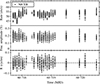 |
Fig. 1. Top panel: NICER 0.3–10 keV light curve of IGR J17511−3057 during the latest outburst starting from February 11, 2025 (MJD 60717.7). The count rate is estimated by collecting 50 s of exposure time. Middle panel: Temporal evolution of the fractional amplitude of the sinusoidal component used to model the source pulse profiles. Bottom panel: Pulse phase residuals in units of phase cycles relative to the best-fitting solution. |
Timing solutions for IGR J17511−3057 during the observed outbursts.
We extracted the spectral products using the nicerl3-spect pipeline tool with the cleaned events in the 0.4–10 keV energy range. We applied the SCORPEON background model version 22 with the option BKGFORMAT=FILE. To perform spectral fitting with enough statistics, we grouped the energy channels to have a minimum of 25 counts per energy bin (GROUPSCALE = 25 and applied the option GROUPTYPE=OPTMIN (Kaastra & Bleeker 2016) from the FTOOLS ftgrouppha. We performed spectral fitting with XSPEC 12.14.0 (Arnaud 1996).
2.2. NuSTAR
NuSTAR observed IGR J17511−3057 (Obs.ID. 91101304002) on February 19, 2025, starting from 15:10 UTC for a total coverage of ∼66.4 ks. After applying the standard screening and filtering procedure with the data analysis software NUSTARDAS from HEASOFT, version 6.33.2, we obtained a cleaned event dataset with a total exposure of ∼37.6 ks. We extracted source and background events from circular regions of radius 120″ and 140″ at the source position and in a source-free region of the same quadrant, respectively. We extracted light curves and spectra (including correlated response files) using the NUPRODUCTS pipeline. Furthermore, we used the lcmath task to create background-subtracted light curves for each NuSTAR FPM and a cumulative one, resulting in a total mean count rate of ∼12.4 cts/s in the 3–80 keV energy range. As reported in Fig. 2, around 30 ks from the beginning of the observation, NuSTAR reveals a sudden and intense increase in X-rays that resembles a typical type-I X-ray burst profile. For our analysis of the coherent X-ray pulsation, we removed data from a 200-s interval centered on the occurrence time of the X-ray burst. We applied barycentric corrections to the NuSTAR photon arrival times by using the BARYCORR tool (DE-405 Solar System ephemeris) with the best available source position reported in Table 1 (Nowak et al. 2009) and applying the latest clock correction file.
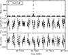 |
Fig. 2. Top panel: NuSTAR Background-subtracted light curve of the latest outburst of IGR J17511−3057 as observed combining data collected by NuSTAR FPMA and FPMB (ObsID. 91101304002) starting from February 19, 2025 (MJD 60725.6). A type-I X-ray burst is detected at around MJD 60725.98. Middle panel: Temporal evolution of the fractional amplitude of the sinusoidal component used to model the source pulse profiles. Bottom panel: Pulse phase residuals in units of phase cycles relative to the best-fitting solution. |
To be able to improve the ephemerides of IGR J17511−3057 during its 2015 outburst, we analyzed the archival NuSTAR observation (obs.ID. 90101001002) performed on April 8, 2015, starting from 20:36 UTC for a total coverage of ∼88.5 ks. Following the same procedure described earlier, we extracted source and background events from circular regions of radius 120″ and 140″ at the source position and in a source-free region of the same quadrant, respectively. We applied the standard screening and filtering procedure and extracted light curves and spectra (including correlated response files) for a total exposure time of ∼46.4 ks using the standard NuSTAR pipelines. A type-I X-ray burst is observed close to the end of the observation. We excluded the event while performing the spin frequency timing analysis. Also for this dataset, we applied barycentric corrections using the BARYCORR tool with the source position reported in Table 1.
2.3. XMM-Newton
We extracted the XMM-Newton observation of IGR J17511−3057 performed on March 26, 2015, at 22:17 UTC for a total coverage of ∼76 ks (Obs.ID. 0770580301). Using the latest version of the XMM-Newton scientific software (SAS v.22.1.0), we extracted the events collected by the EPIC-pn camera operated in timing mode. Following Papitto et al. (2016), we first filtered the data from soft proton flaring episodes, then we extracted the source by selecting only events with the RAWX coordinate within the interval 27–47. We extracted the background filtering events within a three-pixel-wide region centered on the coordinate RAWX = 4. The three type-I X-ray bursts observed during the XMM-Newton observation were excluded while performing the spin frequency timing analysis. For the timing analysis, we reported the EPIC-pn photon arrival times to the Solar System barycenter by using the BARYCEN tool (DE-405 Solar System ephemeris), adopting the best available source position reported in Table 1.
3. Results
3.1. Timing analysis
To perform the timing analysis of the latest outburst of IGR J17511−3057, we started by correcting the NICER and NuSTAR photon arrival times for the binary orbital motion based on the assumption of a circular orbit (see, e.g., Deeter et al. 1981; Burderi et al. 2007). As a starting point, we propagated the orbital ephemeris reported from the previous outburst (see Table 3 in Papitto et al. 2016) and extrapolated the closest value of the time of passage of the ascending node (TASC) to begin looking for possible shifts in time. We then explored the orbital parameter space around the values reported by Papitto et al. (2016), varying TASC by steps of 1 s within its 3σ confidence level interval derived from the 2015 outburst. We searched for coherent pulsations for each set of orbital parameters by applying the epoch-folding method to both datasets. We divided the pulse profile into 20 phase bins and explored the frequency space around v = 244.83395112(3) Hz (the mean spin frequency during the 2015 outburst) with a step of 10−7 Hz for a total of 5001 steps. We recovered strong pulsed signals in both datasets, with the most prominent signal-to-noise ratio (S/N) pulse profile corresponding to a common TASC = 60717.674078 MJD and a frequency of ν = 244.8339503 Hz for both NICER and NuSTAR datasets.
Using the preliminary updated value of TASC and the first guess of the latest spin frequency of the source, we demodulated the photon arrival times for the binary orbit. We created pulse profiles by epoch-folding 50 and 500-s long data segments, for NICER and NuSTAR, respectively, considering the different count rates of the datasets. Using the corresponding mean spin frequency values obtained from the epoch-folding search method, we generated pulse profiles by considering ten phase bins per interval to collect enough photons per bin within the selected time interval. We characterized each pulse profile with a sinusoidal function, from which we extracted the corresponding amplitude and fractional part of the phase residual. When required, we added a second harmonically related sinusoidal component to improve the modeling of the pulse profile. We retained only profiles with statistical significance greater than 3σ. We studied the temporal evolution of the derived pulse phases applying standard phase-coherent timing techniques (see, e.g., Burderi et al. 2007; Sanna et al. 2016, and references therein). We repeated the process until no significant differential corrections were found for the model parameters. In Table 1, we report the best-fitting parameters from the phase-coherent timing analysis. Following Papitto et al. (2016), we estimated the uncertainties on the spin frequency by adding the systematic uncertainty arising from the positional uncertainty in quadrature. The middle and bottom panels of Figs. 1 and 2 show the fractional amplitude and the best-fitting residuals for each time interval explored for NICER and NuSTAR, respectively. The reduced χred2 obtained from the joint fit and the pulse phase best-fit residuals distribution are compatible with the presence of timing noise, widely observed in several AMXPs (see, e.g., Burderi et al. 2006; Papitto et al. 2007; Riggio et al. 2008, 2011a; Patruno & Watts 2021, and references therein). A dedicated consistency check on the phase residuals (power-spectrum and autocorrelation diagnostics) shows no statistically significant low-frequency (“red”) component, indicating that the excess variance is consistent with white noise in the pulse phases. To account for that, the uncertainties on the parameters reported in Table 1 are rescaled by a factor  for a more realistic estimation (see, e.g., Finger et al. 1999)1.
Using the updated ephemeris reported in Table 1, we created an average pulse profile with the highest statistical significance in the 0.3–10.0 keV and 3.0–40.0 keV energy bands for NICER and NuSTAR, respectively. The profiles reported in Fig. 3 are well described by combining three harmonically related sinusoids with a dominant fundamental component.
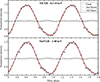 |
Fig. 3. NICER 0.3–10 keV average pulse profiles (top) and 3–40 keV average pulse profiles (bottom) of IGR J17511−3057 generated by folding at the best-fit timing solution reported in Table 1. For both profiles, the best-fitting models (red solid lines) are the superposition of up to three harmonically related sinusoidal components represented in light blue, green, and purple from smaller to higher order, respectively. Two cycles of the pulse profile are shown for clarity. |
The NICER profile (Fig. 3, top panel) shows a background-corrected fractional amplitude of 19%, 1.3%, and 1.1% for the fundamental, second, and third harmonics, respectively. Similarly, the NuSTAR profile is characterized by a background-corrected fractional amplitude of 19.5%, 1.0%, and 1.3% for the fundamental, second, and third harmonics, respectively.
We investigated the energy dependence of the pulse profile for the two datasets. We selected four energy bands for NICER (0.3–1.5 keV, 1.5–4.0 keV, 4.0–6.0 keV and 6.0–10.0 keV) and NuSTAR (3.0–4.0 keV, 4.0–6.0 keV, 6.0–12.0 keV and 12.0–40.0 keV) and folded the corresponding events using the parameters reported in Table 1. The NICER pulse profiles (top four panels in Fig. 4) are well described as the superposition of two harmonically related sinusoidal components, except for the 1.5–4.0 keV where a third harmonic is required to improve the modeling of the profile. The background-corrected fractional amplitude of the fundamental component increases from ∼16% at the lowest energies, and reaches a maximum of ∼21%. The second harmonic shows a linear trend with energy, rising from 1.2% to ∼4%. Interestingly, only for the 1.5–4.0 keV interval, a third harmonic with a fractional amplitude of ∼1.3% (similar to the second harmonic amplitude) is statistically required to improve the pulse profile fit.
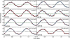 |
Fig. 4. Evolution of the NICER and NuSTAR pulse profiles of IGR J17511−3057 as a function of energy. Pulse profiles are generated by folding at different energy ranges after correcting the photon time-of-arrival for the most updated binary ephemerides reported in Table 1. The best-fitting models (red solid lines) are the superposition of up to two harmonically related sinusoidal components. Two cycles of the pulse profile are shown for clarity. The color-coding follows the convention described in Fig. 3. |
The NuSTAR pulse profiles (bottom four panels in Fig. 4) are well described as the superposition of three harmonically related sinusoidal components, except for the 3.0–4.0 keV, where the third harmonic is not statistically significant. The fractional amplitude of the fundamental component peaks at ∼21.5% in the range 3.0–6.0 keV and decreases to ∼16% at the highest energies. The amplitude of the second harmonic remains constant around ∼1.1% as the energy increases. The profiles extracted at energies above 4.0 keV show the presence of a third harmonic with an amplitude of ∼1.5%, stronger than the second harmonic.
To investigate the long-term evolution of the spin frequency and the orbital parameters of IGR J17511−3057, we improved the accuracy of the source ephemerides reported by Papitto et al. (2016) (based on XMM-Newton) for the 2015 outburst by including a NuSTAR observation performed during the same outburst but never reported so far. We performed the timing analysis following the procedure extensively described above. Results from the study are reported in Table 1 (third column).
Finally, using the same RXTE dataset, we verified the accuracy of the ephemerides reported by Riggio et al. (2011a) by performing a standard phase-coherent timing analysis. The results shown in Table 1 (second column) are compatible within uncertainties with those reported by Riggio et al. (2011a).
3.2. Spectral analysis
This section presents the spectral analysis of NICER and NuSTAR data collected during different phases of the 2025 outburst. Additionally, we examined the time-resolved spectroscopy of the thermonuclear (type-I) X-ray burst observed with NuSTAR.
3.2.1. NICER spectroscopy
A time-averaged spectral analysis was performed using NICER observations of IGR J17511−3057 from February 11–14, 2025. This approach was chosen as the source intensity remained nearly constant, showing only a gradual increase during these observations (top panel of Fig. 1). The 0.4–10 keV NICER spectrum was initially modeled with a simple absorbed power-law with a blackbody component. The photoelectric absorption from the interstellar medium was described with the Tbabs component in XSPEC, with wilm abundances (Wilms et al. 2000) and verner cross-sections (Verner et al. 1996). This model provided a good fit, yielding a reduced chi-square (χred2) of 1.05 for 954 degrees of freedom (hereafter, d.o.f.). Alternatively, we found that a semi-phenomenological Comptonization model ThComp (Zdziarski et al. 2020) with a seed blackbody component can provide an equally good fit, resulting in a χν2 of 1.03 for 954 d.o.f. This model, expressed as Tbabs*(Thcomp*bbodyrad) in XSPEC, was adopted for further analysis of the NICER spectrum ofIGR J17511−3057.
Regardless of the modeling approach, emission residuals were observed around 1.7 keV. Adding a Gaussian emission component at 1.7 keV to the Comptonization-based continuum model successfully accounted for the residuals, with an improvement in the χ2 (Δχ2) of 92.5 for three additional d.o.f. (corresponding to a significance > 9σ). The best-fitting line centroid energy, E0, width, σE, and normalization, N, are 1.69 ± 0.02 keV, 70 ± 20 eV, and 3.3 ± 0.7 × 10⁻⁴ cm−2 s−1, respectively. The equivalent width is 15 ± 4 eV. Weak emission residuals were also observed in the 6–7 keV band. Including a second Gaussian line to account for these residuals improved the fit (Δχ2 = 28 for three additional d.o.f., corresponding to a significance > 4σ). The parameters for the second emission line are, E0 = 6.7 ± 0.2 keV, σE = 0.6 ± 0.2 keV, and N = (4.3 ± 1.1)×10−4 cm−2 s−1, with an equivalent width of 131 ± 86 eV. To assess the statistical significance of both emission features, we performed Monte Carlo simulations using XSPEC’s simftest command. For the 1.7 keV line, only 2 out of 1000 simulated spectra based on the null model showed a fit improvement equal to or greater than that observed in the real data, corresponding to a global p-value of 0.002, suggesting a line significance of 2.9σ. Moreover, for the 6.6 keV line, none of the 1000 simulations matched the observed improvement, implying a global p-value < 0.001 (significance ≥3.3σ). The model parameters from the best fit are also presented in Table 2, while Fig. 5 shows the NICER energy spectrum and corresponding residuals with the best-fittingmodel.
Best-fit spectral parameters for IGR J17511−3057 during the 2025 outburst.
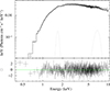 |
Fig. 5. 0.4–10 keV NICER spectrum fitted with an absorbed blackbody with a Comptonization model with two Gaussian emission line components (top), along with the corresponding spectral residuals (bottom). |
Our study primarily focuses on time-averaged spectroscopy, however, we also analyzed four individual NICER observation IDs from the 2025 outburst to evaluate potential variations in spectral parameters. During these observations, spanning February 11–14, 2025, the source unabsorbed flux gradually increased from 3.9 × 10⁻¹⁰ to 4.2 × 10⁻¹⁰ erg s−1 cm−2 with an average flux of (4.03 ± 0.01)×10−10 erg s−1 cm−2 in the 0.5–10 keV as shown in Table 2. The spectral parameters from each observation ID closely match the time-averaged values inthe table.
3.2.2. Semiphenomenological and physical reflection modeling of IGR J17511−3057 with NuSTAR
We extracted the burst-free spectrum from the FPMA and FPMB modules of NuSTAR using observations conducted on February 19–20, 2025. The 3–79 keV spectrum was modeled with an absorbed blackbody combined with a Comptonized component (Thcomp), with the column density fixed at 1.06 × 1022 cm−2, as estimated from the NICER analysis. This model adequately represented the pulsar’s energy continuum, with a χν2 of 1.02 for 1482 d.o.f. A weak indication of emission residuals in the 6–7 keV range was also detected with NuSTAR (Fig. 6). Incorporating a Gaussian emission line into the continuum model improved the fit with a Δχ2 of 48 for three additional d.o.f. The best-fit parameters and their uncertainties at the 90% confidence level are listed in Table 2.
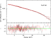 |
Fig. 6. NuSTAR spectrum fitted with an absorbed blackbody with a Comptonization model (top). A weak hint of emission residuals in the 6–7 keV iron band is evident in the corresponding spectral residuals (bottom). |
To explore the evolution of the outburst, we compared the unabsorbed flux in the 0.5–10 keV band obtained from NICER and NuSTAR. During the NuSTAR observation, the flux had decreased by approximately 35–40% compared to the NICER measurements taken between February 11–14, 2025 (Table 2). This decline indicates that the NuSTAR observation occurred during the decay phase of the 2025 outburst of IGR J17511−3057. Furthermore, variations in spectral parameters were observed between these observations(Table 2).
We further investigated the spectral behaviour during the decay phase of IGR J17511−3057 with NuSTAR, using the self-consistent relxillCp reflection model (García et al. 2014; Dauser et al. 2014). This physical model accounts for relativistic reflection from an incident nthcomp continuum. Key model parameters include the photon index (Γ), the accretion disk’s ionization parameter (log ξ), disk density (log N), inclination angle (i), inner and outer disk radii, and iron abundance relative to solar (Afe). The disk emissivity is described by indices q1 and q2. For simplicity, we assumed a single emissivity profile, fixing q1 and q2 to the standard value of 3. In our fit, the outer disk radius was set to 1000 gravitational radii (Rg = GM/c2), with a break radius Rbr at 400 Rg. The dimensionless spin parameter was frozen at 0.7 (Miller et al. 2011; Jaisawal et al. 2019). The choice of spin parameter, whether set to 0 or 0.7, does not significantly affect the derived spectral parameters. Based on the semi-phenomenological modeling with ThComp, the electron temperature (kTe) was fixed at 17 keV during the reflection modeling. Other parameters, such as the inclination angle, inner disk radius, accretion disk density (log N in cm−3), ionization parameter, relative iron abundance, reflection fraction parameter (Reffrac), and the model normalization, were left freeto vary.
The 3–79 keV NuSTAR spectrum was self-consistently described using an absorbed rexillCp model with a fixed absorption column density of 1.06 × 1022 cm−2. This model also yielded a χν2 close to 1, indicating a good fit. Moreover, it also accounted for the weak emission residuals in the 6–7 keV range. The results suggest the presence of moderately ionized reflection, with log ξ of  . The relative iron abundance is poorly constrained, with values ranging between 1 and 9. The fit further indicated a high inclination angle of
  degrees, suggesting a lower limit of the inclination angle greater than 37°. The inner disk radius was constrained to a range of (40–180) Rg, corresponding to (82–370) km, assuming a canonical NS of 1.4 solar mass. The spectral parameters are given in Table 2. Uncertainties on the parameters were estimated for a 90% confidence interval using Markov Chain Monte Carlo (MCMC) chain with the Goodman-Weare algorithm in XSPEC. This simulation employed 2 × 10⁶ chain steps and 20 walkers, discarding the first 1 × 10⁶ steps as burn-in and transient phases. The MCMC corner plot is shown in Fig. A.1.
3.2.3. Broadband spectroscopy with NICER and NuSTAR
Although NICER and NuSTAR observations were not simultaneous, we jointly fitted their data better to constrain the inclination angle and inner disk parameters. We employed an absorbed Comptonized Thcomp model combined with a blackbody component. Initially, this model did not adequately describe the spectra. To address potential spectral evolution between the two datasets, the photon index in the Thcomp model was allowed to vary independently for NICER and NuSTAR. Additionally, a Gaussian feature was incorporated to represent a 1.7 keV emission line. To further investigate the iron line feature, a Diskline component was incorporated. The parameters of the Diskline include the emissivity index, which characterizes the power-law dependence of the disk’s illuminated emissivity profile, scaling as r−β, along with the inner and outer disk radii and the disk inclination (Fabian et al. 1989). For our analysis, the emissivity index was fixed at a value of 3. The smearing parameters derived from the Diskline model were consistent with those obtained using the self-consistent reflection model from the NuSTAR data using relxillCp (see Table 2). The diskline model provided improved constraints, with the inner disk radius estimated in a range of (24–122) Rg, representing a modest improvement compared to the values from the NuSTAR fit (Table 2). The lower bound of the inclination angle was estimated to be 32 degrees without an upper constraint. Other model parameters, such as the photon index derived from the Thcomp model, were consistent with the values obtained from the individual fitting of NICER and NuSTAR. The blackbody emission parameters also match those from the individual fits.
3.2.4. Burst time-resolved spectroscopy
A thermonuclear (type-I) X-ray burst was detected during the NuSTAR observation at an onset time of MJD 60725.98235. The burst reached an average peak count rate of 1500 ± 200 c s−1 in the 3–79 keV range light curve at a bin time of 0.25 s (see top panel of Fig. 7). The profile exhibited a fast rise time of 2 s, followed by an exponential decay time of 8.5 s. The burst spanned a total duration of approximately 25 s, during which the count rate remained above 10% of the peak burst rate. During the rise phase, the burst shows a pause-like structure, similar to those observed in SAX J1808.4-3658 (Bult et al. 2019a) and MAXI J1807+132 (Albayati et al. 2021) with NICER.
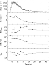 |
Fig. 7. Burst time-resolved spectral parameters. The top panel shows the burst light curve in the 3–79 keV range. The blackbody temperature (kT) and its normalization (BBNorm) are shown in the second and third panels. The bolometric blackbody flux in the 0.1–100 keV range is presented in the fourth panel in the unit of erg s−1 cm−2, whereas the fifth panel shows the value of χred2 from the fit. |
Before studying the burst time-resolved spectroscopy, we extracted a pre-burst spectrum in the same orbit of the burst with an exposure time of 1250 s. The pre-burst spectra from FPMA and FPMB detector modules are fitted using an absorbed blackbody model with a Comptonized ThComp component. The parameters obtained from the pre-burst fit are consistent with the values reported in Table 2 from burst-free persistent emission from NuSTAR. Our pre-burst parameters (at 90% confidence level) are: blackbody temperature kTbb = 0.6 ± 0.1 keV, Norm , ThCompΓ = 1.84 ± 0.01, ThCompkTe = 19.3 ± 4.5, and the flux in 0.5–100 keV = (6.62 ± 0.05) × 10−10 erg s−1 cm−2. The column density was fixed at 1.06 × 1022 cm−2.
We performed time-resolved spectroscopy to investigate the nature of the observed X-ray burst with NuSTAR. We generated 14 time-resolved spectra to successively cover the burst’s rise, peak, and decay phases, each containing a minimum of 1200 counts per interval. The exposure times for these intervals range between 0.75 and 10 s, with a median exposure of 1.125 s. Each burst time-resolved spectrum using data from FPMA and FPMB modules was fitted in the 3–30 keV range with an absorbed blackbody model at a fixed value of the above pre-burst emission parameters and absorption column density. This approach allowed us to incorporate the contribution of persistent accretion emission. The model successfully described the spectra of each time interval. Due to acceptable values of χred2, we did not include a scaling factor to probe any changes in the pre-burst emission during the burst. The scaling factor is considered in the case of the variable persistent emission method, which accounts for the observed soft excess during X-ray bursts after the burst blackbody component (see, e.g., Worpel et al. 2013; Jaisawal et al. 2024). As shown in Fig. 7, a high blackbody temperature of approximately 3 keV was detected around the rise and peak phases of the burst. This temperature exhibited an exponential decline during the decay phase. The blackbody normalization increased during the rise and decay phases, reaching a maximum value of 160 ± 20, corresponding to a blackbody emission radius of 8.7 ± 0.6 km, assuming a distance of 6.9 kpc. The X-ray burst did not show any evidence of photospheric radius expansion. The burst peak flux in the 0.1–100 keV range is estimated to be (5.4 ± 0.4) × 10−8 erg s−1 cm−2. The observed flux matches well with the peak values detected in a range of (3–6.7) × 10−8 erg s−1 cm−2 from a sample of ten X-ray bursts with RXTE (Altamirano et al. 2010). We also calculated the burst fluence by integrating the bolometric blackbody flux over each time interval from time-resolved spectroscopy. This resulted in a burst fluence of (5.1 ± 0.1) × 10−7 erg cm−2. The uncertainties on the burst parameters are given for a 68% confidence level.
3.2.5. Burst oscillations
We searched the NuSTAR burst for oscillations since previously observed X-ray bursts from IGR J17511−3057 have shown burst oscillations (Altamirano et al. 2010). We used data in the 3–40 keV band and performed a sliding time window search. We selected a time range of ∼60 s around the burst and computed FFT power spectra using 4 s intervals. The whole window begins approximately 14 s before the burst rise. For each 4 s interval, we computed the Z2 statistic in a 3 Hz band of frequencies centered around the measured spin frequency. We slide the window by 1/4 of a second to obtain the next time window for the search. We found a strong candidate interval with a peak Z2 power of 38.7 at a frequency consistent with the measured spin frequency. This power value has a single trial chance probability of 4.0 × 10⁻⁹. We used a frequency resolution of 0.01 Hz for a total of 30 measurements across the searched frequency band. We also searched 226 intervals, giving a total of 301 × 226 = 67.424 trials for the search, resulting in an estimate of the chance probability of 2.7 × 10⁻⁴, which is a 3.5σ detection. Fig. 8 shows the contours of Z2 power relative to the burst intensity profile. To check that this significance is not overstated by the strong overlap between adjacent windows and the correlations among closely–spaced frequencies, we ran 50.000 Monte-Carlo bursts that reproduce the observed envelope and were processed through the identical search pipeline. Only two simulations reached a peak power equal to or larger than the real one, implying a global probability of pMC = 4.0 × 10⁻⁵ (equivalent to 3.9σ), fully consistent with a highly significant detection once the true number of independent trials is taken into account. The position of the interval showing the highest Z2 power is consistent with previous measurements of bursts with RXTE (see Altamirano et al. 2010, Fig. 5). We folded the peak Z2 interval from our search using the measured frequency and fit a sinusoid to the resulting pulse profile in order to measure the pulsed amplitude. A sinusoid fits the profile well, and the resulting amplitude is 25 ± 5%. The folded profile, along with the best-fitting model, is shown in Fig. 9.
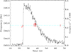 |
Fig. 8. Contours of constant Z2 power shown as a function of time and frequency from our burst oscillation search. Contours are plotted at Z2 levels from 14 to 34 in steps of 4. The horizontal dashed line (cyan) denotes the measured spin frequency. |
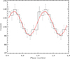 |
Fig. 9. Folded pulse profile from the 4 s interval which yielded the peak Z2 power in our search. The best-fitting sinusoidal model is also plotted (red). |
4. Discussion and conclusions
We present the temporal and spectral properties of the AMXP pulsar IGR J17511−3057 during its 2025 outburst, obtained through our investigation of the available NICER and NuSTAR datasets.
4.1. Pulse profile energy dependence
The average pulse profiles, which collect all available events in the 0.3–10 keV and 3.0–40.0 keV bands for NICER and NuSTAR, respectively, are shown in Fig. 3. Both best-fit models required three harmonics to successfully describe the pulse profiles, with a dominant fundamental component characterized by a fractional amplitude of ∼19% in the two datasets. The second and third harmonics, both displaying a similar fractional amplitude of ∼1%, are required to model small asymmetries of the profiles. This is consistent with the modeling of the pulse profiles of the previous outburst, where (due to higher statistics) a fourth harmonic was significantly detected (see, e.g., Papitto et al. 2010, 2016; Riggio et al. 2011a). Thus far, harmonically rich pulse profiles have not been considered standard among AMXPs; apart from IGR J17511−3057, only XTE J1807−294 (see, e.g., Patruno et al. 2010), Swift J1749.4−2807 (Altamirano et al. 2011; Sanna et al. 2022a), MAXI J1957+032 (Sanna et al. 2022b), IGR J16597−3704 (Sanna et al. 2018b), and IGR J17591−2342 (Sanna et al. 2018c; Kuiper et al. 2020) have required three or more components.
In Fig. 4, we show the energy dependence of the pulse profiles obtained by folding NICER and NuSTAR datasets with the ephemerides reported in Table 1 in different energy bands. The profile amplitude, dominated by the fundamental component, increases with energy with a common maximum of ∼21% for the two datasets in the band 3.0–6.0 keV. This is compatible with what was reported from the previous outbursts from the RXTE and XMM-Newton observations of the source. The observed fractional amplitude is among the highest observed so far in AMXPs, other systems showing large fractional amplitude (above 15%) are IGR J17379−3747 (see, e.g., Sanna et al. 2018d; Bult et al. 2019b) SWIFT J1749.4−2807 (see, e.g., Altamirano et al. 2011; Sanna et al. 2022a), XTE J1807−294 (Patruno et al. 2010), and IGR J17591−2342 (Sanna et al. 2020). According to Poutanen & Beloborodov (2006), large fractional amplitudes could reflect an inclination angle > 45° for rotators with relatively small misalignment angles (< 20°). It is worth noting that for a two hot spot scenario, the maximum pulse amplitude is predicted to occur when the sum of the two angles is close to 90°. For IGR J17511−3057, this is consistent with the constraint on the inclination (38° −68°) reported by Papitto et al. (2010), as well as from the results discussed in Sect. 3.2.2, based on the modeling of the reflection continuum spectrum.
Interestingly, the harmonic content of the profile increases with energy. Both the second and the third (when detected) harmonics have their amplitude increase with the rise in energy. The 6.0–10.0 keV NICER pulse profile appears significantly affected by the increase in the second harmonic component. The third harmonic is detected in a few, relatively high-energy intervals, where its amplitude is similar to that of the second harmonic. This could be an observational bias related to the number of photons in the selected intervals. As shown in Papitto et al. (2016) and (Riggio et al. 2011a), increasing the statistics allows us to significantly detect the third (and even a fourth) component at similar energy ranges, where the component shows a fractional amplitude around 1% or less.
The energy dependence of the fundamental pulse amplitude of IGR J17511−3057 resembles that of other AMXPs such as SAX J1748.9−2021 (Patruno et al. 2009b; Sanna et al. 2016), IGR J00291+5934 (Falanga et al. 2005; Sanna et al. 2017a), XTE J1807−294 (Kirsch et al. 2004; Patruno et al. 2010), XTE J1751−305 (Falanga & Titarchuk 2007), and IGR J17494−3030 (Ng et al. 2021). This behaviour may be ascribable to strong Comptonization of the beamed radiation, required to extend the pulsed spectrum to higher energies (see, e.g., Falanga & Titarchuk 2007, and references therein).
4.2. Long-term spin evolution
We performed phase-coherent timing analysis of the previous two outbursts of IGR J17511−3057 detected since its discovery, obtaining consistent results with previous reported analysis (see, e.g., Papitto et al. 2010, 2016; Riggio et al. 2011a). To determine possible secular evolution of the spin frequency, we combined previous outbursts with the updated ephemeris of the source obtained with NICER and NuSTAR (Table 1). We adopted a linear model to describe the temporal evolution of the three spin frequency values, obtaining a best-fit reduced χred2 ∼ 154, with one d.o.f. and a spin frequency derivative of  Hz/s. Although the general trend shows a clear decrease in the spin frequency, the large value of the reduced chi-squared indicates that a simple linear spin-down model is not statistically acceptable. This discrepancy most likely arises because the spin frequency evolves due to the transient accretion-driven torques associated with the active accretion phases during the outbursts, which a constant linear spin-down assumption cannot adequately capture. We further investigated the frequency evolution by accounting for the spin-up phases during the 2009 and 2015 outbursts. We independently estimated the frequency variation, Δν2009 − 2015 and Δν2015 − 2025, comparing the end of the first outburst with the beginning of the second, as well as comparing the end of the second with the beginning of the third outburst, respectively. Following Riggio et al. (2011a), for the 2009 outburst, we assumed a duration of 24 days and a spin-up frequency derivative of
  Hz/s. Considering the spin frequency reported in Table 1 as a proxy of the value at beginning of the 2015 outburst, we obtained Δν2009 − 2015 = ( − 1.25 ± 0.05)×10−6 Hz, which corresponds to
  Hz/s. For the 2015 outburst, we found no direct evidence of frequency derivative, only an upper limit on the order of
  Hz/s (3σ confidence level). Considering a duration of 22 days (see Fig. 1 from Papitto et al. 2016), we estimated −6.0 × 10⁻⁷ Hz < Δν2015 − 2025 < −0.4 × 10⁻⁷ Hz, corresponding to a secular spin derivative
  . It remains unclear what causes the discrepancy between the two estimates of spin derivatives during the quiescence phases. However, the poor knowledge of the possible accretion torque during the 2015 outburst in terms of strength and duration does not allow a better constraint.
Nonetheless, we note that similar values of spin-down derivative during the quiescence phase have been reported for a handful of AMXPs, such as SAX J1808.4−3658 ( Hz/s; Illiano et al. 2023a), IGR J17498−2921 (
 Hz/s; Illiano et al. 2024), XTE J1751−305 (
 Hz/s; Riggio et al. 2011b), IGR J00291+5934 (
 Hz/s; Patruno 2010; Papitto et al. 2011b; Hartman et al. 2011), and SWIFT J1756.9−2508 (
 Hz/s; Sanna et al. 2018a).
Interpreting  as the spin derivative during the rotation-powered phase of IGR J17511−3057 in quiescence, we can combine the rotational energy loss rate with the rotating magnetic dipole emission to infer the magnetic field strength at the NS polar caps. For a rotating dipole in the presence of matter, we can approximate the dipolar magnetic moment of the NS as
 (1)
(1)
where α is the angle between the rotation and magnetic axes (see, e.g., Spitkovsky 2006, and references therein) and I45 is the moment of inertia of the NS in units of 1045 g cm2, while ν245 and  are in units of IGR J17511−3057 spin frequency, and spin frequency derivative, respectively. Without prior knowledge of the angle α, we can constrain the magnetic moment μ between the extremes of α = 0 deg (aligned rotator) and α = 90 deg (orthogonal rotator). Substituting the relevant spin frequency and its secular derivative in Eq. (1), we can limit the NS magnetic moment to be 5.6 × 1026 G cm3 < μ < 7.9 × 1026 G cm3. Adopting the FPS equation of state for a 1.4 M⊙ NS and RNS = 1.14 × 106 cm (NS, see e.g., Friedman & Pandharipande 1981; Pandharipande & Ravenhall 1989), we can constrain the magnetic field strength at the magnetic polar caps,
  , to the interval 7.6 × 10⁸ G < BPC < 1.1 × 10⁹ G, in accordance with the estimates from disk and stellar magnetic field interaction reported by Mukherjee et al. (2015). However, the spin-up rate on the order of (1.45 ± 0.16)×10−13 Hz/s reported by Riggio et al. (2011a) from the 2009 outburst, suggests we are estimating only a lower limit on the magnetic field strength of the source, since we are ignoring the likely increase in the spin frequency of IGR J17511
 3057 during outburst phases, where it is expected to be increasing due the matter and angular momentum transferred onto its surface.
4.3. Secular orbital period evolution
We started by collecting the most accurate estimates of the orbital period from previous outbursts to investigate the secular evolution of the orbital period. More specifically, from Table 1, we considered Porb, 2009 = 12487.5118(4) s, Porb, 2015 = 12487.507(1) s, and Porb, 2025 = 12487.505(2) s. We modeled the orbital evolution with a linear function from which we obtained an estimate of the period derivative of Ṗorb = −1.81(67) × 10−11 s/s with a reduced χred2 = 3.5 for one d.o.f. The relatively large uncertainty does not allow us to determine the orbital evolution unambiguously, although it seems to point towards a fast contraction on long timescales.
We explored the possibility of improving the constraint on the orbital period derivative by applying a coherent-orbital-phase analysis using the measurements of the epoch of passage of the ascending node (TASC) in the three observed outbursts. More specifically, from Table 1, we considered TASC, 2009 = 55088.0320286(6) MJD, TASC, 2015 = 57107.858808(1) MJD, and TASC, 2025 = 60717.674090(3) MJD. Moreover, to be able to determine the number of elapsed orbital cycles (N) and calculate the delays with respect to the predicted times TASC, PRE(N) = TASC, 0 + N Porb, 0 (see, e.g., Papitto et al. 2005; Di Salvo et al. 2008; Hartman et al. 2009; Burderi et al. 2009; Iaria et al. 2015), we defined Porb, 0 = Porb, 2009. Following the method described in Sanna et al. (2018a), we find that the number of elapsed cycles between the outbursts is unambiguously determined, verifying the condition required to apply the timing technique. For each outburst we determine the quantity ΔTASC = TASC, OBS − TASC, PRE and modeled it using the quadratic function as
 (2)
(2)
where δTASC, 0 represents the correction to TASC, 2009 adopted as a reference value, δPorb, 0 is the correction to the orbital period, and Ṗorb is the orbital-period derivative.
Because we only have three data points and three parameters in our quadratic model, a standard least-squares approach would yield no d.o.f. and thus no meaningful uncertainty estimates. Instead, we employed a Bayesian method with suitable priors to constrain the parameter space and obtain reliable intervals from the resulting posterior distributions. We estimated the best-fit parameters and their uncertainties by sampling the posterior distribution with a Markov Chain Monte Carlo (MCMC) algorithm. Specifically, we adopted flat (uniform) priors for the parameters δTASC, 0 and δPorb, 0 based on the accuracy of the available measurements. Values significantly larger than the two quantities would have led to clear observational signatures during the 2009 outburst, thereby justifying our chosen prior bounds. We employed the MCMC emcee ensemble sampler (Foreman-Mackey et al. 2013) to generate sufficient draws from the joint posterior. We then derived the following median parameter values and their 1σ intervals from the 16th and 84th percentiles of the resulting marginalized posterior distributions: δTASC, 0 = < 0.15 s (3σ c.l.), δPorb, 0 = 6.26(1)×10−3 s, Ṗorb=−2.55(7) × 10−11 s/s (see Fig. 10). This result implies a more accurate estimate of the orbital period of Porb = 12487.51806(2) s. It is worth noting that the orbital period derivative is compatible with the estimate obtained from the direct comparison of the orbital periods. However, given the accuracy achieved in measuring the orbital period during the 2009 outburst, we should have been able to directly measure the orbital period obtained from the TASC secular evolution. This crucial point requires further investigation to understand at which level secular changes in TASC trace back the orbital evolution.
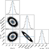 |
Fig. 10. Posterior probability distributions and pairwise covariances of the parameters ΔTASC, ΔPorb, and Ṗorb obtained from the Bayesian MCMC analysis of the secular evolution of the TASC from the three outbursts of IGR J17511−3057 (corner plot). See Sect. 4.3 for more details. Solid lines delimit the 1σ and 2σ confidence level regions. |
Erratic orbital period variation has been reported for several binary pulsars classified as MSPs. At least three black widow pulsars (characterized by a < 0.1 M⊙ low-mass, partially evaporated or oblate, companion star) exhibited complex orbital changes requiring high-order orbit derivatives to be described. Among them, PSR J0023+0923 interestingly displays changes in the orbital period, measured in terms of large erratic drifts of the time of the predicted TASC both in radio and X-rays (see, e.g., Bak Nielsen et al. 2020). Similar behaviour has been reported for red back pulsars (with relatively more massive, 0.1–0.4 M⊙, non-degenerate companions). Systems such as PSR J2339-0533 show alternating increases and decreases in the orbital period over timescales of a few years. Cyclic changes in the companion star’s gravitational quadrupole moment, likely associated with magnetic activity cycles, have been proposed to explain the peculiar orbital behaviour (see, e.g., Pletsch & Clark 2015, and references therein). The transitional MSP PSR J1023+0038 shows erratic behaviour of the time of passage at the ascending node, with variations of tens of seconds over timescales of years (see, e.g., Archibald et al. 2013, 2015; Jaodand et al. 2016; Papitto et al. 2019; Burtovoi et al. 2020; Illiano et al. 2023b). Long-term timing studies revealed significant timing noise and orbital variations for red backs in globular clusters. For example, orbital changes in MSPs located in Terzan 5 have been interpreted with a combination of cluster-induced accelerations and intrinsic processes such as mass transfer or torques from the companion star (see, e.g., Rosenthal et al. 2025).
Currently, significant orbital period derivatives have been measured for three other AMXPs, namely, SAX J1808.4−3658 (see e.g., Di Salvo et al. 2008; Patruno 2017; Sanna et al. 2017b; Bult et al. 2020; Illiano et al. 2023a), SWIFT J1749.4−2807 (Sanna et al. 2022a), and IGR J17062−6143 (Bult et al. 2021), all suggesting a fast orbital expansion. For five more AMXPs, uncertainties are such that it is not yet possible to determine whether the orbits are secularly expanding or shrinking (see, e.g., Sanna et al. 2016, 2017a, 2018a,d; Bult et al. 2018; Patruno 2017).
Considering all the previously discussed caveats, we notice that both independent methods investigated to extrapolate the secular orbital evolution suggest a fast contraction of the binary system. If confirmed, this could be compatible with a scenario in which angular momentum loss due to gravitational wave radiation dominates. Although theoretically predicted, this scenario has never been observationally confirmed for AMXPs so far. If we define the orbital evolution timescale as τ = Porb/Ṗorb and we consider an orbital period derivative on the order of Ṗorb ≃ −2 × 10⁻¹¹ s/s, we find that IGR J17511−3057 is evolving with τ ∼ 20 Myr. For comparison, we can consider the evolutionary timescale reported by Paczyński (1971):
 (3)
(3)
where q = m2/m1 is the binary mass ratio, m1 and m2 are the NS and the secondary masses in units of solar masses, and Porb, days is the orbital period expressed in days. Adopting m2 in the range 0.15–0.44 M⊙ (see, e.g., Papitto et al. 2010) and m1 in the range 1.0–2.5 M⊙, we find a predicted evolutionary timescale for IGR J17511−3057 in the range τgw = 3 − 15 Gyr. This is almost three orders of magnitude longer than our estimate.
Following Di Salvo et al. (2008), we can express the orbital period derivative of the system in terms of the angular momentum lost and transferred in the system. More specifically, if we express the orbital angular momentum of the system as: Jorb = [Ga/(M1 + M2)]1/2M1M2 (where G is the Gravitational constant, and a is the orbital separation), and define − Ṁ2 the mass transferred by the secondary (which can be accreted onto the NS via conservative mass transfer or t can be lost from the system, non-conservative mass transfer), we can express this as
![Mathematical equation: $$ \begin{aligned} \frac{\dot{P}_{\rm orb}}{P_{\rm orb}} = 3 \left[\frac{\dot{J}}{J_{\rm orb}} - \frac{\dot{M}_2}{M_2} \; g(\beta ,q,\alpha )\right], \end{aligned} $$](/articles/aa/full_html/2025/11/aa55734-25/aa55734-25-eq34.gif) (4)
(4)
where g(β, q, α) = 1 − βq − (1 − β)(α + q/3)/(1 + q), with β the fraction of mass lost by the secondary and accreted by the NS, α the specific angular momentum of the mass lost by the system, and  the possible losses of angular momentum from the system.
According to theory, orbital angular momentum can be dissipated via gravitational waves and magnetic braking emissions. The latter being dominant for systems with longer orbital periods (starting from Porb > 2 h; see, e.g., Verbunt 1993; Tauris 2001). Combining the two mechanisms, we can express the angular momentum loss as
![Mathematical equation: $$ \begin{aligned} \left(\frac{\dot{J}}{J_{\rm orb}}\right)_{\rm GR+MB}=-2.1\times 10^{-17}m_1~m_{2}~m^{-1/3}P_{\rm orb,3h}^{-8/3}[1+T_{\rm MB}], \end{aligned} $$](/articles/aa/full_html/2025/11/aa55734-25/aa55734-25-eq36.gif) (5)
(5)
where m1, m2, and m represent the primary, secondary, and total mass in units of solar masses. Porb, 3h is the orbital period in units of three hours and TMB represents the magnetic braking torque. Following Iaria et al. (2018), TMB can be parameterized as:
 (6)
(6)
where k represents the gyration radius of the secondary star and f is a dimensionless parameter which can be considered either as f = 0.73 (Skumanich 1972) or f = 1.78 (Smith 1979).
According to Papitto et al. (2010), the companion star can be limited in the interval M2/M⊙ = 0.15 − 0.44, assuming M1 = 1.4 M⊙. Assuming k = 0.45 (see. e.g., Wadhwa et al. 2024), and f = 0.73 (which maximizes the magnetic braking effect), Eq. (5) applied to IGR J17511−3057 limits  between −9 × 10⁻¹⁷ s−1 (m2 = 0.15) and −4 × 10⁻¹⁶ s−1 (m2 = 0.44), which according to Eq. (4), could account up to ∼5% or ∼20% of the observed Ṗorb/Porb, respectively.
Recent developments, including the convection and rotation-boosted (CARB) magnetic braking model proposed by Van & Ivanova (2019), offer more physically motivated descriptions of angular momentum losses in low-mass, fully convective secondary stars. Unlike earlier approaches that often oversimplify or neglect convection effects, CARB predicts enhanced magnetic braking for rapidly rotating, fully convectivecompanions.
Applying the CARB model for a companion mass of m2 ∼ 0.2 M⊙, with a wind mass-loss rate of Ṁw ∼ 7.5 × 10⁻¹⁴ M⊙/yr, a stellar radius R ∼ 0.3 R⊙ (corresponding to the secondary Roche lobe radius for the assumed companion mass), a luminosity of L ∼ 0.02 L⊙ (parameters extrapolated from Reimers’ prescription for mass-loss rates due to stellar winds Reimers 1975), and assuming a rotation period on the order of the binary period due to tidally locked rotation, yields a magnetic braking torque ranging widely from approximately −3 × 1046 g cm2/s2, corresponding to a  s−1, which is several orders of magnitude larger than the observed effect measured in this work. However, it is worth noting from Eq. (6) in Van & Ivanova (2019), the strong dependence of
  on the companion rotation rate Ω. Releasing the tidally locked rotation condition for the companion star (and hypothetically considering rotation rates on the order of the tens of days) could provide the required amount of angular momentum losses to match the observed Ṗorb/Porb. Nevertheless, the very short tidal-synchronization timescales in AMXPs make any sustained departure from synchronous (tidally locked) rotation highly improbable, rendering these slower-rotation scenarios largely hypothetical for IGR J17511−3057. Future observational tests targeting precise measurements of orbital decay rates and companion rotation periods would be essential to differentiate between traditional MB models and the CARB scenario, ultimately refining our understanding of angular momentum evolution in AMXPs.
We go on to consider the contribution of mass transfer ( ) by exploring the two extreme scenarios: conservative (β = 1) and totally non-conservative (β = 0) mass transfer. The former implies g(β, q, α) = 1 − q, hence,
  , ignoring the effect of
  . The requested rate of mass transfer from the companion would then range between 2.9 × 10⁻⁹ M⊙/yr and 7.1 × 10⁻⁹ M⊙/yr, considering the possible secondary mass interval. Defining LX = GṀMNS/RNS as the luminosity emitted by the NS due to the accretion of matter, we can estimate an expected constant luminosity from the NS over the long-term timescales that is between 3 × 1037 erg s−1 and 7.4 × 1037 erg s−1 for MNS = 1.4 M⊙ and RNS = 1.14 × 106 cm. While this value is on the same order of magnitude as the estimate found from the spectral modeling of the source during the outburst (Papitto et al. 2010, 2016; Bozzo et al. 2010), it is not compatible with the average luminosity of IGR J17511−3057 over a sixteen-year baseline from which we extrapolated the orbital evolution, making the conservative mass-transfer scenario unfeasible. It is worth noting that even accounting for the largest loss of angular momentum combining gravitational waves and magnetic braking (∼20% of the observed Ṗorb/Porb), the conservative mass-transfer scenario would require a long-term average luminosity that is still too high (∼1037 erg s−1) to be missed during the quiescencephases.
On the other hand, a non-conservative mass transfer scenario requires continuous mass transfer from the secondary, with only partial accretion onto the NS surface. Assuming roughly an average outburst duration of one month for three observed episodes, we could define a source duty cycle of ∼0.015 over the sixteen-year baseline investigated here. Therefore, assuming that the inferred mass accretion rate during the outburst represents the average long-term mass transfer rate from the secondary, ∼0.015 can also be interpreted as the fraction of accreted matter β previously defined. As a first-order approximation, given the small value of β, we can consider the totally nonconservative mass-transfer scenario (β = 0), for which g(0, q, α) = (1 − α + 2q/3)/(1 + q). Since Ṗorb/Porb is negative, g(0, q, α) needs to be positive. Assuming the NS mass of 1.4 M⊙ and exploring the companion mass in the range 0.15–0.44, we can investigate the location at which the mass needs to be ejected from the system, in terms of its specific angular momentum carried away, to produce an orbital evolution on the order of Ṗorb/Porb. We find that ejecting matter with an α parameter in the range 1.9 − 2.1 solves Eq. (4), allowing, at least theoretically, to explain the inferred fast secular contraction of the binary system with a combination of loss of mass and angular momentum from the system. However, several open questions remain with respect to i) what causes the matter to be ejected from the secondary during the quiescence phase and, if the radiation pressure is generated from a rotation-powered pulsar turning on (see, e.g., Di Salvo et al. 2008; Burderi et al. 2009, and references therein), why there is only evidence of only one AMXP (IGR J18245–2452 Papitto et al. 2013) swinging between accretion and rotation-powered states (see, e.g., Burderi et al. 2009; Iacolina et al. 2010, for more details on the topic); ii) why there is no evidence of the ejected matter around thecompanion star.
Alternative processes, such as gravitational quadrupole coupling between the companion star and the binary orbit (see, e.g., Applegate 1992; Applegate & Shaham 1994), have been proposed to describe periodic orbital variations on timescales of years for different MPSs (Doroshenko et al. 2001; Pletsch & Clark 2015). Magnetically driven changes in the mass distribution of the donor star modify the companion’s oblateness, changing the gravitational interaction within the binary system and inducing orbital period variations on dynamical timescales. While plausible, the application of this scenario for IGR J17511−3057 is currently limited by the lack of observational evidence for a long-term orbital modulation, with only three outbursts available forinvestigation.
Confirming this secular trend is crucial to investigating further theoretical frameworks that could explain such a peculiar orbital evolution. Therefore, future outbursts of the IGR J17511−3057 are required to validate the system’s orbital period derivative.
4.4. Spectral properties
We studied the spectral characteristics of IGR J17511−3057 during its 2025 outburst using NICER and NuSTAR. The spectra were well described by a semi-phenomenological model consisting of an absorbed blackbody and a thermally Comptonized component (ThComp). NICER observations revealed an average unabsorbed flux of 4 × 10⁻¹⁰ erg s−1 cm−2 in the 0.5–10 keV range, which gradually increased from 3.9 × 10⁻¹⁰ to 4.2 × 10⁻¹⁰ ergs−1 cm−2 between February 11 and 14, 2025. The source flux declined to 2.52 × 10⁻¹⁰ erg s−1 cm−2 in the same energy range as observed by NuSTAR on February 19–20, 2025, with a corresponding bolometric flux (0.5–100 keV) of 6.7 × 10⁻¹⁰ erg s−1 cm−2 or a luminosity of 3.8 × 1036 erg s−1 cm−2 at a distance of 6.9 kpc. This flux decline suggests that the NuSTAR observation occurred during the decay phase of the 2025 outburst. In comparison, during the 2009 (Bozzo et al. 2010) and 2015 (Papitto et al. 2015) outbursts, the peak flux in the 0.5–10 keV band was measured in the range of (5–7) × 10−10 erg s−1 cm−2, slightly higher than the flux observed by NICER in 2025. Assuming similar outburst behaviour, the outburst likely peaked between the observation gap of NICER and NuSTAR (see also Sguera 2025b).
The spectral shape of IGR J17511−3057 is dominated by a hard power-law component with an index around 1.6–1.8 and an electron temperature of ≥15 keV. We also observed an emission line feature at 1.7 keV with NICER, consistent with the Kα transition of neutral Si. The same feature has been observed in other NICER observations (see, e.g., Marino et al. 2022; Illiano et al. 2024), suggesting an instrumental origin. Additionally, both instruments detected weak emission residuals around 6.6 ± 0.2 keV, with a central line energy consistent with the Kα transition of neutral or He-like Fe. This line was relatively broader, with a width of 0.6 ± 0.2 keV. XMM-Newton also observed an iron line at 6.65 ± 0.25 keV with a relatively broad width of > 0.56 keV during the decay phase of the 2015 outburst, with an inner accretion disk radius truncated at > 40 km (Papitto et al. 2016). To examine the emission from the accretion disk and the origin of the 6.6 keV line, we modeled the NuSTAR spectrum with the self-consistent reflection model relxillCp. This allowed us to constrain the inclination angle of the system to be greater than 37°, which aligns with earlier measurements from the 2015 outburst (Papitto et al. 2016). The modeling also indicated that the inner disk radius is truncated in the range of (40–180) Rg, corresponding to (82–370) km, inferred assuming a canonical NS mass of 1.4 solar mass. A slightly better constrained value was found in the range of (24–122) Rg, corresponding to (50–252) km from broadband fitting using Diskline. The lower limit of inner disk radius is almost closer to the predicted NS co-rotation radius of ∼43 km. We found a moderate ionization of the accretion disk, with a log ξ of 2.7 ± 0.7, supporting an ionized iron emission line from the inner region of the accretion disk. The line broadness can be explained by considering the effect of the Doppler shift and the NS gravitational field.
4.5. Type-I X-ray burst
A thermonuclear X-ray burst was observed during the NuSTAR observation of IGR J17511−3057. The burst exhibited a rapid rise time of 2 s, followed by an exponential decay of 8.5 s, with a total duration of 25 s. Typically, bursts fueled by hydrogen-rich material are longer, lasting up to hundreds of seconds (Bildsten 2000). The short duration of this burst suggests a fuel composition deficient in hydrogen. However, it could also imply a higher CNO metallicity, as noted by Falanga et al. (2011), based on the observed burst recurrence time of 7 hours in the 2009 outburst. The NuSTAR burst occurred at a pre-burst flux of (6.62 ± 0.05) × 10−10 erg s−1 cm−2, corresponding to a luminosity of 3.8 × 1036 erg s−1 at a distance of 6.9 kpc. This suggests that the NS was accreting at the mass accretion rate of about 1% of the Eddington limit (Kuulkers et al. 2003). Furthermore, our timing studies revealed oscillations during the rise and decay phases of the NuSTAR burst around 244.85 Hz, with a significance level of 3.6σ and a fractional amplitude of 25 ± 5%.
Our burst time-resolved spectroscopy revealed a peak blackbody temperature of ∼3 keV, cooling to 1.2 keV by the end of the burst. The blackbody normalization at the peak temperature corresponds to an emission radius of 5.4 ± 0.5 km. During the decay phase, a higher emission radius of 8.7 ± 0.6 km, consistent with the NS radius, was observed. The burst lacked evidence of photospheric radius expansion, indicating that the observed peak flux of (5.4 ± 0.4) × 10−8 erg s−1 cm−2 was below the Eddington limit. This peak value is consistent with non-PRE bursts previously observed with RXTE and INTEGRAL/JEM-X, which ranged between (3–6.7) × 10−8 erg s−1 cm−2 and provided an upper limit of the distance (Altamirano et al. 2010; Falanga et al. 2011). The fluence of the NuSTAR burst was estimated to be (5.1 ± 0.1) × 10−7 erg cm−2, corresponding to a net energy release of 2.9 × 1039 erg. Finally, we note that no evidence of soft excesses was detected during the burst.
We stress that the  rescaling is a pragmatic convention, which is appropriate only when the unmodeled variance is temporally white, and not a formally derived likelihood treatment.
Acknowledgments
A.P. is supported by INAF (Research Grant ‘Uncovering the optical beat of the fastest magnetized NSs 620 (FANS)’), the Italian Ministry of University and Research (MUR) PRIN 2020 Grant 2020BRP57Z, ‘Gravitational and Electromagnetic-wave Sources in the Universe with current and next-generation detectors (GEMS)’) and Fondazione Cariplo/Cassa Depositi e Prestiti, grant no. 2023-2560. M.N. is a Fonds de Recherche du Québec – Nature et Technologies (FRQNT) postdoctoral fellow. C.M. is supported by INAF (Research Grant ‘Uncovering the optical beat of the fastest magnetized neutron stars 620 (FANS)’) and the Italian Ministry of University and Research (MUR) (PRIN 2020, Grant 2020BRP57Z, ‘Gravitational and Electromagnetic-wave Sources in the Universe with current and next-generation detectors (GEMS)’). T.B. is supported in part by the Turkish Republic, Directorate of Presidential Strategy and Budget project, 2016K121370.
References
- Albayati, A. C., Altamirano, D., Jaisawal, G. K., et al. 2021, MNRAS, 501, 261 [Google Scholar]
- Alpar, M. A., Cheng, A. F., Ruderman, M. A., & Shaham, J. 1982, Nature, 300, 728 [NASA ADS] [CrossRef] [Google Scholar]
- Altamirano, D., Watts, A., Linares, M., et al. 2010, MNRAS, 409, 1136 [Google Scholar]
- Altamirano, D., Cavecchi, Y., Patruno, A., et al. 2011, ApJ, 727, L18 [NASA ADS] [CrossRef] [Google Scholar]
- Applegate, J. H. 1992, ApJ, 385, 621 [Google Scholar]
- Applegate, J. H., & Shaham, J. 1994, ApJ, 436, 312 [NASA ADS] [CrossRef] [Google Scholar]
- Archibald, A. M., Stairs, I. H., Ransom, S. M., et al. 2009, Science, 324, 1411 [Google Scholar]
- Archibald, A. M., Kaspi, V. M., Hessels, J. W. T., et al. 2013, ApJ, submitted [arXiv:1311.5161] [Google Scholar]
- Archibald, A. M., Bogdanov, S., Patruno, A., et al. 2015, ApJ, 807, 62 [NASA ADS] [CrossRef] [Google Scholar]
- Arnaud, K. A. 1996, in Astronomical Data Analysis Software and Systems V, eds. G. H. Jacoby, & J. Barnes, ASP Conf. Ser., 101, 17 [NASA ADS] [Google Scholar]
- Bak Nielsen, A.-S., Janssen, G. H., Shaifullah, G., et al. 2020, MNRAS, 494, 2591 [Google Scholar]
- Baldovin, C., Kuulkers, E., Ferrigno, C., et al. 2009, ATel, 2196, 1 [NASA ADS] [Google Scholar]
- Bassa, C. G., Patruno, A., Hessels, J. W. T., et al. 2014, MNRAS, 441, 1825 [Google Scholar]
- Bildsten, L. 2000, in Cosmic Explosions: Tenth AstroPhysics Conference, eds. S. S. Holt, & W. W. Zhang, AIP Conf. Ser., 522, 359 [Google Scholar]
- Bozzo, E., Ferrigno, C., Falanga, M., et al. 2010, A&A, 509, L3 [NASA ADS] [CrossRef] [EDP Sciences] [Google Scholar]
- Bozzo, E., Kuulkers, E., Bazzano, A., et al. 2015, ATel, 7275, 1 [NASA ADS] [Google Scholar]
- Bult, P., Altamirano, D., Arzoumanian, Z., et al. 2018, ApJ, 864, 14 [Google Scholar]
- Bult, P., Jaisawal, G. K., Güver, T., et al. 2019a, ApJ, 885, L1 [CrossRef] [Google Scholar]
- Bult, P., Markwardt, C. B., Altamirano, D., et al. 2019b, ApJ, 877, 70 [Google Scholar]
- Bult, P., Chakrabarty, D., Arzoumanian, Z., et al. 2020, ApJ, 898, 38 [CrossRef] [Google Scholar]
- Bult, P., Strohmayer, T. E., Malacaria, C., Ng, M., & Wadiasingh, Z. 2021, ApJ, 912, 120 [Google Scholar]
- Burderi, L., Di Salvo, T., Menna, M. T., Riggio, A., & Papitto, A. 2006, ApJ, 653, L133 [NASA ADS] [CrossRef] [Google Scholar]
- Burderi, L., Di Salvo, T., Lavagetto, G., et al. 2007, ApJ, 657, 961 [NASA ADS] [CrossRef] [Google Scholar]
- Burderi, L., Riggio, A., di Salvo, T., et al. 2009, A&A, 496, L17 [NASA ADS] [CrossRef] [EDP Sciences] [Google Scholar]
- Burtovoi, A., Zampieri, L., Fiori, M., et al. 2020, MNRAS, 498, L98 [NASA ADS] [CrossRef] [Google Scholar]
- Chakrabarty, D., Morgan, E. H., Muno, M. P., et al. 2003, Nature, 424, 42 [CrossRef] [PubMed] [Google Scholar]
- Dauser, T., Garcia, J., Parker, M. L., Fabian, A. C., & Wilms, J. 2014, MNRAS, 444, L100 [Google Scholar]
- Deeter, J. E., Boynton, P. E., & Pravdo, S. H. 1981, ApJ, 247, 1003 [NASA ADS] [CrossRef] [Google Scholar]
- Di Salvo, T., & Sanna, A. 2020, ArXiv e-prints [arXiv:2010.09005] [Google Scholar]
- Di Salvo, T., Burderi, L., Riggio, A., Papitto, A., & Menna, M. T. 2008, MNRAS, 389, 1851 [NASA ADS] [CrossRef] [Google Scholar]
- Doroshenko, O., Löhmer, O., Kramer, M., et al. 2001, A&A, 379, 579 [NASA ADS] [CrossRef] [EDP Sciences] [Google Scholar]
- Fabian, A. C., Rees, M. J., Stella, L., & White, N. E. 1989, MNRAS, 238, 729 [Google Scholar]
- Falanga, M., & Titarchuk, L. 2007, ApJ, 661, 1084 [NASA ADS] [CrossRef] [Google Scholar]
- Falanga, M., Kuiper, L., Poutanen, J., et al. 2005, A&A, 444, 15 [NASA ADS] [CrossRef] [EDP Sciences] [Google Scholar]
- Falanga, M., Kuiper, L., Poutanen, J., et al. 2011, A&A, 529, A68 [NASA ADS] [CrossRef] [EDP Sciences] [Google Scholar]
- Finger, M. H., Bildsten, L., Chakrabarty, D., et al. 1999, ApJ, 517, 449 [NASA ADS] [CrossRef] [Google Scholar]
- Foreman-Mackey, D., Hogg, D. W., Lang, D., & Goodman, J. 2013, PASP, 125, 306 [Google Scholar]
- Friedman, B., & Pandharipande, V. R. 1981, Nucl. Phys. A, 361, 502 [Google Scholar]
- Galloway, D. K., Chakrabarty, D., Morgan, E. H., & Remillard, R. A. 2002, ApJ, 576, L137 [NASA ADS] [CrossRef] [Google Scholar]
- Galloway, D. K., Goodwin, A. J., & Keek, L. 2017, PASA, 34, e019 [Google Scholar]
- García, J., Dauser, T., Lohfink, A., et al. 2014, ApJ, 782, 76 [Google Scholar]
- Hartman, J. M., Patruno, A., Chakrabarty, D., et al. 2008, ApJ, 675, 1468 [NASA ADS] [CrossRef] [Google Scholar]
- Hartman, J. M., Patruno, A., Chakrabarty, D., et al. 2009, ApJ, 702, 1673 [NASA ADS] [CrossRef] [Google Scholar]
- Hartman, J. M., Galloway, D. K., & Chakrabarty, D. 2011, ApJ, 726, 26 [NASA ADS] [CrossRef] [Google Scholar]
- Iacolina, M. N., Burgay, M., Burderi, L., Possenti, A., & di Salvo, T. 2010, A&A, 519, A13 [NASA ADS] [CrossRef] [EDP Sciences] [Google Scholar]
- Iaria, R., Di Salvo, T., Gambino, A. F., et al. 2015, A&A, 582, A32 [NASA ADS] [CrossRef] [EDP Sciences] [Google Scholar]
- Iaria, R., Gambino, A. F., Di Salvo, T., et al. 2018, MNRAS, 473, 3490 [CrossRef] [Google Scholar]
- Illiano, G., Papitto, A., Sanna, A., et al. 2023a, ApJ, 942, L40 [NASA ADS] [CrossRef] [Google Scholar]
- Illiano, G., Papitto, A., Ambrosino, F., et al. 2023b, A&A, 669, A26 [NASA ADS] [CrossRef] [EDP Sciences] [Google Scholar]
- Illiano, G., Papitto, A., Marino, A., et al. 2024, A&A, 691, A189 [NASA ADS] [CrossRef] [EDP Sciences] [Google Scholar]
- Jaisawal, G. K., Wilson-Hodge, C. A., Fabian, A. C., et al. 2019, ApJ, 885, 18 [NASA ADS] [CrossRef] [Google Scholar]
- Jaisawal, G. K., Bostancı, Z. F., Boztepe, T., et al. 2024, ApJ, 975, 67 [NASA ADS] [CrossRef] [Google Scholar]
- Jaodand, A., Archibald, A. M., Hessels, J. W. T., et al. 2016, ApJ, 830, 122 [Google Scholar]
- Kaastra, J. S., & Bleeker, J. A. M. 2016, A&A, 587, A151 [NASA ADS] [CrossRef] [EDP Sciences] [Google Scholar]
- Kirsch, M. G. F., Mukerjee, K., Breitfellner, M. G., et al. 2004, A&A, 423, L9 [NASA ADS] [CrossRef] [EDP Sciences] [Google Scholar]
- Kuiper, L., Tsygankov, S. S., Falanga, M., et al. 2020, A&A, 641, A37 [NASA ADS] [CrossRef] [EDP Sciences] [Google Scholar]
- Kuulkers, E., den Hartog, P. R., in’t Zand, J. J. M., et al. 2003, A&A, 399, 663 [NASA ADS] [CrossRef] [EDP Sciences] [Google Scholar]
- Lewin, W. H. G., van Paradijs, J., & Taam, R. E. 1993, Space Sci. Rev., 62, 223 [CrossRef] [Google Scholar]
- Marino, A., Anitra, A., Mazzola, S. M., et al. 2022, MNRAS, 515, 3838 [CrossRef] [Google Scholar]
- Markwardt, C. B., Altamirano, D., Swank, J. H., et al. 2009, ATel, 2197, 1 [NASA ADS] [Google Scholar]
- Miller, J. M., Miller, M. C., & Reynolds, C. S. 2011, ApJ, 731, L5 [Google Scholar]
- Miller-Jones, J. C. A., Russell, D. M., & Migliari, S. 2009, ATel, 2232, 1 [Google Scholar]
- Mukherjee, D., Bult, P., van der Klis, M., & Bhattacharya, D. 2015, MNRAS, 452, 3994 [NASA ADS] [CrossRef] [Google Scholar]
- Ng, M., Ray, P. S., Bult, P., et al. 2021, ApJ, 908, L15 [NASA ADS] [CrossRef] [Google Scholar]
- Ng, M., Boztepe, T., Sanna, A., et al. 2025, ATel, 17032, 1 [Google Scholar]
- Nowak, M. A., Paizis, A., Wilms, J., et al. 2009, ATel, 2215, 1 [NASA ADS] [Google Scholar]
- Paczyński, B. 1971, ARA&A, 9, 183 [Google Scholar]
- Pandharipande, V. R., & Ravenhall, D. G. 1989, in NATO Advanced Science Institutes (ASI) Series B, eds. M. Soyeur, H. Flocard, B. Tamain, & M. Porneuf, 205, 103 [Google Scholar]
- Papitto, A., Menna, M. T., Burderi, L., et al. 2005, ApJ, 621, L113 [Google Scholar]
- Papitto, A., di Salvo, T., Burderi, L., et al. 2007, MNRAS, 375, 971 [NASA ADS] [CrossRef] [Google Scholar]
- Papitto, A., Menna, M. T., Burderi, L., di Salvo, T., & Riggio, A. 2008, MNRAS, 383, 411 [Google Scholar]
- Papitto, A., Riggio, A., di Salvo, T., et al. 2010, MNRAS, 407, 2575 [Google Scholar]
- Papitto, A., Bozzo, E., Ferrigno, C., et al. 2011a, A&A, 535, L4 [NASA ADS] [CrossRef] [EDP Sciences] [Google Scholar]
- Papitto, A., Riggio, A., Burderi, L., et al. 2011b, A&A, 528, A55 [NASA ADS] [CrossRef] [EDP Sciences] [Google Scholar]
- Papitto, A., Ferrigno, C., Bozzo, E., et al. 2013, Nature, 501, 517 [NASA ADS] [CrossRef] [Google Scholar]
- Papitto, A., de Martino, D., Belloni, T. M., et al. 2015, MNRAS, 449, L26 [NASA ADS] [CrossRef] [Google Scholar]
- Papitto, A., Bozzo, E., Sanchez-Fernandez, C., et al. 2016, A&A, 596, A71 [NASA ADS] [CrossRef] [EDP Sciences] [Google Scholar]
- Papitto, A., Ambrosino, F., Stella, L., et al. 2019, ApJ, 882, 104 [NASA ADS] [CrossRef] [Google Scholar]
- Patruno, A. 2010, ApJ, 722, 909 [NASA ADS] [CrossRef] [Google Scholar]
- Patruno, A. 2017, ApJ, 839, 51 [Google Scholar]
- Patruno, A., & Watts, A. L. 2021, Astrophys. Space Sci. Lib., 461, 143 [NASA ADS] [CrossRef] [Google Scholar]
- Patruno, A., Wijnands, R., & van der Klis, M. 2009a, ApJ, 698, L60 [NASA ADS] [CrossRef] [Google Scholar]
- Patruno, A., Altamirano, D., Hessels, J. W. T., et al. 2009b, ApJ, 690, 1856 [NASA ADS] [CrossRef] [Google Scholar]
- Patruno, A., Hartman, J. M., Wijnands, R., Chakrabarty, D., & van der Klis, M. 2010, ApJ, 717, 1253 [NASA ADS] [CrossRef] [Google Scholar]
- Patruno, A., Bult, P., Gopakumar, A., et al. 2012, ApJ, 746, L27 [NASA ADS] [CrossRef] [Google Scholar]
- Pletsch, H. J., & Clark, C. J. 2015, ApJ, 807, 18 [Google Scholar]
- Poutanen, J., & Beloborodov, A. M. 2006, MNRAS, 373, 836 [NASA ADS] [CrossRef] [Google Scholar]
- Reimers, D. 1975, in Problems in Stellar Atmospheres and Envelopes, eds. B. Baschek, W. H. Kegel, & G. Traving, 229 [Google Scholar]
- Riggio, A., Di Salvo, T., Burderi, L., et al. 2008, ApJ, 678, 1273 [NASA ADS] [CrossRef] [Google Scholar]
- Riggio, A., Papitto, A., Burderi, L., et al. 2011a, A&A, 526, A95 [NASA ADS] [CrossRef] [EDP Sciences] [Google Scholar]
- Riggio, A., Burderi, L., di Salvo, T., et al. 2011b, A&A, 531, A140 [NASA ADS] [CrossRef] [EDP Sciences] [Google Scholar]
- Rosenthal, A. C., Ransom, S. M., Corcoran, K. A., et al. 2025, ApJ, 982, 170 [Google Scholar]
- Sanna, A., Burderi, L., Riggio, A., et al. 2016, MNRAS, 459, 1340 [Google Scholar]
- Sanna, A., Pintore, F., Bozzo, E., et al. 2017a, MNRAS, 466, 2910 [NASA ADS] [CrossRef] [Google Scholar]
- Sanna, A., Di Salvo, T., Burderi, L., et al. 2017b, MNRAS, 471, 463 [NASA ADS] [CrossRef] [Google Scholar]
- Sanna, A., Pintore, F., Riggio, A., et al. 2018a, MNRAS, 481, 1658 [NASA ADS] [CrossRef] [Google Scholar]
- Sanna, A., Bahramian, A., Bozzo, E., et al. 2018b, A&A, 610, L2 [NASA ADS] [CrossRef] [EDP Sciences] [Google Scholar]
- Sanna, A., Ferrigno, C., Ray, P. S., et al. 2018c, A&A, 617, L8 [NASA ADS] [CrossRef] [EDP Sciences] [Google Scholar]
- Sanna, A., Bozzo, E., Papitto, A., et al. 2018d, A&A, 616, L17 [NASA ADS] [CrossRef] [EDP Sciences] [Google Scholar]
- Sanna, A., Burderi, L., Gendreau, K. C., et al. 2020, MNRAS, 495, 1641 [Google Scholar]
- Sanna, A., Burderi, L., Di Salvo, T., et al. 2022a, MNRAS, 514, 4385 [Google Scholar]
- Sanna, A., Bult, P., Ng, M., et al. 2022b, MNRAS, 516, L76 [NASA ADS] [CrossRef] [Google Scholar]
- Sguera, V. 2025a, ATel, 17029, 1 [Google Scholar]
- Sguera, V. 2025b, ATel, 17061, 1 [Google Scholar]
- Skumanich, A. 1972, ApJ, 171, 565 [Google Scholar]
- Smith, M. A. 1979, PASP, 91, 737 [Google Scholar]
- Spitkovsky, A. 2006, ApJ, 648, L51 [Google Scholar]
- Strohmayer, T., & Bildsten, L. 2006, in Compact Stellar X-ray Sources, eds. W. H. G. Lewin, & M. van der Klis, 39, 113 [NASA ADS] [CrossRef] [Google Scholar]
- Tauris, T. M. 2001, in Evolution of Binary and Multiple Star Systems, eds. P. Podsiadlowski, S. Rappaport, A. R. King, F. D’Antona, & L. Burderi, ASP Conf. Ser., 229, 145 [NASA ADS] [Google Scholar]
- Torres, M. A. P., Jonker, P. G., Steeghs, D., et al. 2009, ATel, 2233, 1 [Google Scholar]
- Van, K. X., & Ivanova, N. 2019, ApJ, 886, L31 [NASA ADS] [CrossRef] [Google Scholar]
- Verbunt, F. 1993, ARA&A, 31, 93 [NASA ADS] [CrossRef] [Google Scholar]
- Verner, D. A., Ferland, G. J., Korista, K. T., & Yakovlev, D. G. 1996, ApJ, 465, 487 [Google Scholar]
- Wadhwa, S. S., Landin, N. R., Arbutina, B., et al. 2024, MNRAS, 535, 2494 [Google Scholar]
- Watts, A. L. 2012, ARA&A, 50, 609 [Google Scholar]
- Watts, A. L., Altamirano, D., Markwardt, C. B., & Strohmayer, T. E. 2009, ATel, 2199, 1 [Google Scholar]
- Wijnands, R., & van der Klis, M. 1998, Nature, 394, 344 [CrossRef] [Google Scholar]
- Wilms, J., Allen, A., & McCray, R. 2000, ApJ, 542, 914 [Google Scholar]
- Worpel, H., Galloway, D. K., & Price, D. J. 2013, ApJ, 772, 94 [NASA ADS] [CrossRef] [Google Scholar]
- Zdziarski, A. A., Szanecki, M., Poutanen, J., Gierliński, M., & Biernacki, P. 2020, MNRAS, 492, 5234 [NASA ADS] [CrossRef] [Google Scholar]
Appendix A: MCMC results from the reflection modeling
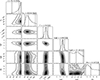 |
Fig. A.1. MCMC results from the reflection modeling of NuSTAR data. The modeling parameters are inclination angle (i), inner disk radius (Rin) in units of gravitational radii, photon index (Γ), the accretion disk’s ionization parameter (log ξ), disk density (log N), and iron abundance relative to solar (Afe). The uncertainties on parameters are given for a 90% confidence range. |
All Tables
All Figures
|
Fig. 1. Top panel: NICER 0.3–10 keV light curve of IGR J17511−3057 during the latest outburst starting from February 11, 2025 (MJD 60717.7). The count rate is estimated by collecting 50 s of exposure time. Middle panel: Temporal evolution of the fractional amplitude of the sinusoidal component used to model the source pulse profiles. Bottom panel: Pulse phase residuals in units of phase cycles relative to the best-fitting solution. |
| In the text | |
|
Fig. 2. Top panel: NuSTAR Background-subtracted light curve of the latest outburst of IGR J17511−3057 as observed combining data collected by NuSTAR FPMA and FPMB (ObsID. 91101304002) starting from February 19, 2025 (MJD 60725.6). A type-I X-ray burst is detected at around MJD 60725.98. Middle panel: Temporal evolution of the fractional amplitude of the sinusoidal component used to model the source pulse profiles. Bottom panel: Pulse phase residuals in units of phase cycles relative to the best-fitting solution. |
| In the text | |
|
Fig. 3. NICER 0.3–10 keV average pulse profiles (top) and 3–40 keV average pulse profiles (bottom) of IGR J17511−3057 generated by folding at the best-fit timing solution reported in Table 1. For both profiles, the best-fitting models (red solid lines) are the superposition of up to three harmonically related sinusoidal components represented in light blue, green, and purple from smaller to higher order, respectively. Two cycles of the pulse profile are shown for clarity. |
| In the text | |
|
Fig. 4. Evolution of the NICER and NuSTAR pulse profiles of IGR J17511−3057 as a function of energy. Pulse profiles are generated by folding at different energy ranges after correcting the photon time-of-arrival for the most updated binary ephemerides reported in Table 1. The best-fitting models (red solid lines) are the superposition of up to two harmonically related sinusoidal components. Two cycles of the pulse profile are shown for clarity. The color-coding follows the convention described in Fig. 3. |
| In the text | |
|
Fig. 5. 0.4–10 keV NICER spectrum fitted with an absorbed blackbody with a Comptonization model with two Gaussian emission line components (top), along with the corresponding spectral residuals (bottom). |
| In the text | |
|
Fig. 6. NuSTAR spectrum fitted with an absorbed blackbody with a Comptonization model (top). A weak hint of emission residuals in the 6–7 keV iron band is evident in the corresponding spectral residuals (bottom). |
| In the text | |
|
Fig. 7. Burst time-resolved spectral parameters. The top panel shows the burst light curve in the 3–79 keV range. The blackbody temperature (kT) and its normalization (BBNorm) are shown in the second and third panels. The bolometric blackbody flux in the 0.1–100 keV range is presented in the fourth panel in the unit of erg s−1 cm−2, whereas the fifth panel shows the value of χred2 from the fit. |
| In the text | |
|
Fig. 8. Contours of constant Z2 power shown as a function of time and frequency from our burst oscillation search. Contours are plotted at Z2 levels from 14 to 34 in steps of 4. The horizontal dashed line (cyan) denotes the measured spin frequency. |
| In the text | |
|
Fig. 9. Folded pulse profile from the 4 s interval which yielded the peak Z2 power in our search. The best-fitting sinusoidal model is also plotted (red). |
| In the text | |
|
Fig. 10. Posterior probability distributions and pairwise covariances of the parameters ΔTASC, ΔPorb, and Ṗorb obtained from the Bayesian MCMC analysis of the secular evolution of the TASC from the three outbursts of IGR J17511−3057 (corner plot). See Sect. 4.3 for more details. Solid lines delimit the 1σ and 2σ confidence level regions. |
| In the text | |
|
Fig. A.1. MCMC results from the reflection modeling of NuSTAR data. The modeling parameters are inclination angle (i), inner disk radius (Rin) in units of gravitational radii, photon index (Γ), the accretion disk’s ionization parameter (log ξ), disk density (log N), and iron abundance relative to solar (Afe). The uncertainties on parameters are given for a 90% confidence range. |
| In the text | |
Current usage metrics show cumulative count of Article Views (full-text article views including HTML views, PDF and ePub downloads, according to the available data) and Abstracts Views on Vision4Press platform.
Data correspond to usage on the plateform after 2015. The current usage metrics is available 48-96 hours after online publication and is updated daily on week days.
Initial download of the metrics may take a while.