| Issue |
A&A
Volume 703, November 2025
|
|
|---|---|---|
| Article Number | A42 | |
| Number of page(s) | 17 | |
| Section | Extragalactic astronomy | |
| DOI | https://doi.org/10.1051/0004-6361/202556017 | |
| Published online | 05 November 2025 | |
Temperature-based radial metallicity gradients in nearby galaxies
1
Astronomisches Rechen-Institut, Zentrum für Astronomie der Universität Heidelberg, Mönchhofstraße 12-14, D-69120 Heidelberg, Germany
2
Space Telescope Science Institute, 3700 San Martin Drive, Baltimore, MD 21218, USA
3
Universidad Nacional Autónoma de México, Instituto de Astronomía, AP 70-264, CDMX 04510, México
4
INAF – Osservatorio Astrofisico di Arcetri, Largo E. Fermi 5, I-50157 Firenze, Italy
5
Department of Physics, Astronomy Section, University of Trieste, Via G.B. Tiepolo, 11, I-34143 Trieste, Italy
6
European Southern Observatory, Avenida Alonso de Cordoba 3107, Casilla 19, Santiago 19001, Chile
7
Department of Physics and Astronomy, University of Wyoming, Laramie, WY 82071, USA
8
Department of Astronomy, University of Cape Town, Rondebosch 7701, Cape Town, South Africa
9
Universität Heidelberg, Zentrum für Astronomie, Institut für Theoretische Astrophysik, Albert-Ueberle-Str 2, D-69120 Heidelberg, Germany
10
Research School of Astronomy and Astrophysics, Australian National University, Canberra, ACT 2611, Australia
11
Universität Heidelberg, Interdisziplinäres Zentrum für Wissenschaftliches Rechnen, Im Neuenheimer Feld 205, D-69120 Heidelberg, Germany
12
Harvard-Smithsonian Center for Astrophysics, 60 Garden Street, Cambridge, MA 02138, USA
13
Elizabeth S. and Richard M. Cashin Fellow at the Radcliffe Institute for Advanced Studies at Harvard University, 10 Garden Street, Cambridge, MA 02138, USA
14
Department of Physics, Tamkang University, No.151, Yingzhuan Rd., Tamsui Dist., New Taipei City 251301, Taiwan
15
Departamento de Física de la Tierra y Astrofísica, Universidad Complutense de Madrid, E-28040, Spain
16
Sub-department of Astrophysics, Department of Physics, University of Oxford, Keble Road, Oxford OX1 3RH, UK
⋆ Corresponding author: This email address is being protected from spambots. You need JavaScript enabled to view it.
Received:
18
June
2025
Accepted:
28
July
2025
Abstract
Context. Gas-phase abundances provide insights into the baryon cycle, with radial gradients and 2D metallicity distributions tracking how metals are built up and redistributed across galaxy disks over cosmic time.
Aims. We use a catalog of 22 958 H II regions across 19 nearby spiral galaxies to examine how precisely the radial abundance gradients can be traced when using only the [N II] λ5755 electron temperature as a proxy for temperature-based, direct method metallicities.
Methods. Using 534 direct detections of the temperature sensitive [N II] λ5755 auroral line, we measured gradients in 15 of the galaxies. Leveraging our large catalog of individual H II regions, we carried out a stacking procedure in bins of the H II region [N II] λ6583 luminosity and radius to recover stacked radial gradients.
Results. We found a good agreement between the metallicity gradients from the stacked spectra and those gradients from individual regions and those from strong-line methods. In addition, particularly in the stacked Te[N II] measurements, some galaxies show very low (< 0.05 dex) scatter in metallicities, indicative of a well-mixed ISM. We examined the individual high confidence (S/N > 5) outliers and identified 13 regions across nine galaxies with anomalously low metallicities, although this is not strongly reflected in the strong-line method metallicities. By stacking arm and interarm regions, we found no systematic evidence for offsets in metallicity between these environments, suggesting that enrichment within spiral arms is due to very localized processes.
Conclusions. This work demonstrates the potential to systematically exploit the single [N II] λ5755 auroral line for detailed gas-phase abundance studies of galaxies. It provides strong validation of previous results, based on the strong-line calibrations, of a well-mixed ISM across typical star-forming spiral galaxies.
Key words: ISM: abundances / HII regions / galaxies: abundances
© The Authors 2025
 Open Access article, published by EDP Sciences, under the terms of the Creative Commons Attribution License (https://creativecommons.org/licenses/by/4.0), which permits unrestricted use, distribution, and reproduction in any medium, provided the original work is properly cited.
This article is published in open access under the Subscribe to Open model. This email address is being protected from spambots. You need JavaScript enabled to view it. to support open access publication.
1. Introduction
Chemical abundances are commonly used as a cosmic clock, since heavy elements are only produced within stars and must be returned to the surrounding interstellar medium (ISM) to pollute and enrich the next generation of stars (Maiolino & Mannucci 2019). In the gas-phase, the oxygen abundance (metallicity) is commonly measured from the rich suite of strong oxygen and hydrogen emission lines produced within photoionized H II regions (Kewley et al. 2019). A detailed study of these metallicities offers a snapshot of the instantaneous metal content in the galaxy at a given position. Radial metallicity gradients are commonly observed in present day galaxies, with enriched gas located towards the galaxy center and the radial decrease well fit by a linear slope (Pilyugin et al. 2014; Sánchez et al. 2014; Belfiore et al. 2017), sometimes with evidence of inflection points or breaks (Sánchez-Menguiano et al. 2016, 2018). While there are different possible physical interpretations for these gradients, they are generally thought to reflect the inside-out growth of galaxies, modified by a complex interplay of outflow-driven removal of metal-rich gas and accretion of metal-poor gas (Dalcanton 2007; Bresolin et al. 2012; Andrews et al. 2017; also see Johnson et al. 2025), along with radial gas flows and other internal processes (e.g., Mollá et al. 2019; Palla et al. 2020, 2024; Prantzos et al. 2023). In this way, deviations from simple linear trends provide insights into some of the key stellar feedback and cosmological processes that are thought to regulate galaxy evolution.
Within the past decade, a rich variety of integral field unit (IFU) spectroscopic instruments and new surveys have provided a remarkable view into the 2D gas-phase metallicity distribution, as mapped across thousands of individual galaxies (e.g., CALIFA, Sánchez et al. 2012; SAMI, Bryant et al. 2015; MaNGA, Bundy et al. 2015). However at kpc scales, most of these studies blend H II regions with each other and with surrounding diffuse ionized gas, introducing biases into the inferred metallicities and metallicity gradients (Poetrodjojo et al. 2019). For smaller samples of nearby (D < 100 Mpc) galaxies, metallicities can be obtained with much higher precision at the locations of individual H II regions (Rosales-Ortega et al. 2011; Blanc et al. 2013), with recent surveys providing measurements for thousands of H II regions per galaxy (e.g., Kreckel et al. 2019; Rousseau-Nepton et al. 2019; Grasha et al. 2022; Groves et al. 2023). With such a high density of metallicity measurements, it has become possible to search for higher order azimuthal variations in the metal distribution and connect the sites of metal formation with mixing and diffusion processes in detail, with a particular focus on variations between galactic environments (Ho et al. 2017; Kreckel et al. 2020; Sánchez-Menguiano et al. 2020; Williams et al. 2022; Bresolin et al. 2025).
There are many methods available to infer the metallicity of an HII region from its emission lines (Maiolino & Mannucci 2019; Kewley et al. 2019), each of which comes with advantages and disadvantages. Obtaining large statistical samples of metallicity measurements generally requires the use of “strong-line” methods (for a review of various methods, see Peimbert et al. 2017). These rely on some combination of bright emission lines (e.g., Hα, Hβ, [O II] λ3727, [O III] λ5007, [N II] λ6583, and [S II] λλ6717,6731), making implicit assumptions about the underlying physical conditions of the nebula, such as the relation between metallicity, ionization parameter, and temperature (Morisset et al. 2025). These prescriptions are calibrated either empirically against sets of nebulae, where electron temperatures (Te) and densities are measured (using the Te-method defined below), or against photoionization models for a range of conditions (e.g., ionization parameter, ISM pressure, etc.) to recover a measurement of 12 + log(O/H) for a wide range of H II region properties. This is in contrast to the Te -method (often called the direct method), where collisionally excited, temperature-sensitive auroral lines are used in combination with lower energy transitional lines to measure Te (e.g., [O III] λ4363 and [O III] λ5007, [N II] λ5755 and [N II] λ6583, [S III] λ6312, and [S II] λ6716,6731). Measuring Te makes it possible to constrain the expected line emissivities, and recover different ionic abundances (e.g., O+/H, O++/H).
The internal structure of H II regions, typically unresolved in external galaxies, arises as radiation from young massive stars ionizes the surrounding gas, creating distinct ionization zones, arranged roughly by their ionization energy. This layered structure reflects the energy distribution of the radiation field. By measuring lines for multiple ions, it is then possible to obtain abundance measurements for individual ionization zones within each nebula and infer the total oxygen abundance (Berg et al. 2020). However, these auroral lines are faint, making up only a few percent of the flux observed in the strong lines; hence, they are typically only observed in the brightest H II regions, requiring dedicated deep observations to recover measurements for samples of ∼10 s of H II regions per galaxy (e.g., Berg et al. 2020). It is worth noting that even these auroral collisionally excited line (CEL) Te-based metallicities are not perfectly understood and they also show systematic offsets from the metallicity inferred using even fainter recombination lines (RL) (Esteban et al. 2014; Toribio San Cipriano et al. 2016; Skillman et al. 2020; Méndez-Delgado et al. 2022; Chen et al. 2024). The 0.1–0.3 dex offset between these two physically grounded methods is known as the abundance discrepancy factor (ADF), which is often attributed to unresolved temperature fluctuations within the nebula (Peimbert 1967; Méndez-Delgado et al. 2023a), reflecting the challenges involved in obtaining a precise understanding of the detailed physics regulating line emission in H II regions.
Recently, the PHANGS-MUSE survey obtained ∼100 pc scale optical IFU coverage of 19 star-forming spiral galaxies (Emsellem et al. 2022), isolating individual star-forming complexes and providing a homogeneous spectroscopic catalog of ∼20 000 H II regions (Groves et al. 2023). This includes coverage of the [N II] λ5755, [S II] λ6312, and [O II] λλ7320,7330 auroral lines. Brazzini et al. (2024) carried out a careful, tailored fitting of these faint lines, and found 95 H II regions with all three lines detected. Rickards Vaught et al. (2024) carried out follow-up observations of seven galaxies to provide coverage of the [O III] λ4363 auroral line, but given the high metallicity of the sample, was only able to obtain detections in 26 (6%) of the H II regions observed. These intensive efforts to fully map the ionization zones within large samples of nebulae demonstrate the challenges of building large databases of H II regions where detailed Te-based abundance measurements are possible.
A simplified approach is possible if one ion could be identified with a temperature representative of the larger ionized volume. Méndez-Delgado et al. (2023a) used the DESIRED catalog (Méndez-Delgado et al. 2023b) to explore temperature relations across a sample of H II regions with exceptionally deep spectra and found that Te[N II] alone provides a remarkably accurate constraint on the metallicity across a wide range of physical conditions. This is extremely convenient within the context of the PHANGS-MUSE results. Brazzini et al. (2024) found that within the ∼20 000 PHANGS-MUSE H II regions, [N II] λ5755 was the most commonly detected auroral line, with measurements obtained for 969 (about 4%) of the H II regions. Overall, [S II] λ6312 was the least commonly detected, found in < 1% of H II regions. Although ∼3% have [O II] λλ7320,7330, the reliability of these detections is questionable as they are heavily blended with bright sky lines in this wavelength range.
In this work, we focus on exploiting detections of the [N II] λ5755 line, as it represents the strongest and best detected auroral line in our sample, to recover direct metallicities of HII regions and investigate radial trends across the disk of our galaxies. We also explore approaches that stack multiple H II region spectra to improve the detection rate of this line and expand our analysis. Additionally, [N II] λ5755/λ6584 is less susceptible to errors from reddening corrections and telluric emission or absorption, compared to other temperature diagnostics such as [S III] λ6312/λ9069 and [O II] λ7330/λ3728.
In Section 2, we describe the optical spectroscopic data used in this study, the H II region catalog, and our stacking approach. In Section 3 we present our Te[N II] measurements, from individual and stacked H II regions, along with the inferred radial metallicity gradients. We also explore the outliers and environmental variations. In Section 4, we validate our choice of strong-line prescription for these systems, consider the utility of Te[N II] as a direct method abundance diagnostic, and discuss the lack of strong environmental variations. We present our conclusions in Section 5.
2. Data
2.1. PHANGS-MUSE spectroscopy
Our sample of 19 star-forming nearby (D < 20 Mpc) galaxies observed with MUSE (Bacon et al. 2010) is listed in Table 1. A full description of the observations and data reduction is provided in Emsellem et al. (2022) and key characteristics of the data set are summarized below.
General properties of the PHANGS-MUSE galaxies.
The MUSE instrument provides optical integral field unit (IFU) spectroscopic imaging across a wide ∼1′ field of view. The resulting spectra cover ∼4800–9300 Å at a spectral resolution of R ∼ 2000 (Bacon et al. 2017). In our sample, typical seeing of ∼0.7″ corresponds to physical scales of 50–100 pc, sufficient to isolate individual H II regions from surrounding nebulae and diffuse ionized gas. As our target galaxies are nearby and extended on the sky, they were typically mosaicked with between 3–15 MUSE pointings to achieve extended coverage of the star-forming disk.
While all observations were taken using the Wide-Field Mode, eight of the galaxies were observed using Ground Layer Adaptive Optics (Arsenault et al. 2008; Ströbele et al. 2012) to improve the seeing, and increase the spatial resolution. As this employs sodium lasers, a notch filter removes emission from 5820–5970 Å. For galaxies with systemic velocities of more than ∼2000 km s−1, depending on the disk rotation this can redshift [N II] λ5755 line emission close enough to the notch that accurate recovery of the line flux cannot be guaranteed. This principally affects NGC 4254, and explains the small number of detections in that galaxy.
2.2. Nebular catalog and H II region selection
From the Hα emission in these 19 galaxies, a catalog of ∼20 000 H II regions were identified and characterized, as detailed in Santoro et al. (2022) and Groves et al. (2023). Integrated spectra are constructed for each nebula that combine data from all MUSE spaxels associated with the region. These integrated spectra were fit using the penalized PiXelFitting (pPXF) package (Cappellari & Emsellem 2004; Cappellari 2017) with a combination of single stellar population (SSP) models (E-MILES, Vazdekis et al. 2016) and Gaussian components for strong emission lines (e.g., Hβ, [O III], Hα, [N II], and [S II]). This results in stellar population models, as well as line flux and line kinematic measurements for each nebula in the catalog. All line fluxes are dereddened by using the Hα/Hβ line ratio to infer E(B − V), assuming an intrinsic Balmer ratio of Hα/Hβ = 2.86, RV = 3.1, and an O’Donnell (1994) extinction curve. Extinction corrected Hα luminosities, L(Hα) are calculated assuming the distances listed in Table 1.
Using diagnostic line ratios (e.g., BPT; Baldwin et al. 1981), we classified a subset of the nebulae as “H II regions” when we can robustly attribute the line emission to photoionization via the following line ratio criteria. Following Groves et al. (2023), we required these regions to fall below the Kauffmann et al. (2003) diagnostic curve in the [O III]/Hβ versus [N II]/Hα BPT diagrams and below the Kewley et al. (2006) diagnostic curve in the [O III]/Hβ versus [S II]/Hα BPT diagrams, with S/N > 5 in all lines. Where [O I] is detected with S/N > 5, we further required the regions to fall below the Kewley et al. (2006) diagnostic curve in the [O I]/Hβ versus [S II]/Hα BPT diagram. We excluded regions that were not fully contained within the field of view and regions overlapping with foreground stars. To avoid the AO notch filter masking 5820–5970 Å we excluded any regions with measured Hα velocities greater than 2345 km s−1. Finally, we excluded regions flagged as residing in the galaxy center environment (Querejeta et al. 2021), as they often have unphysically large physical sizes, due to difficulties in deblending clustered star formation within nuclear rings. Taking these criteria into account, we were left with a sample of 20 809 H II regions, with between 367 and 2196 H II regions identified per galaxy.
The gas-phase oxygen abundance, 12 + log(O/H), has been characterized for each of these regions using the Pilyugin & Grebel (2016) S calibration (Scal), an empirical metallicity prescription that has been shown to provide accurate metallicities for individual H II regions with high precision compared to other prescriptions available in the literature (Ho 2019; Metha et al. 2021). Radial gradients for each galaxy were calculated in Groves et al. (2023) and they are in agreement within the reported uncertainties despite the slightly different H II region selection criteria applied in this work. Subtracting the radial gradient, we can then calculate the offset from the radial gradient, Δ(O/H), for each H II region. All galaxies were well characterized by these simple linear radial gradients, which we characterized by calculating σ(O/H), the standard deviation of Δ(O/H) across the H II regions in the galaxy, finding typical values of 0.03–0.06 dex. This is larger than the typical statistical uncertainties of 0.01 dex determined by propagating the errors associated with the line flux measurements.
As the [N II] λ5755 line is typically ∼0.5% of the strength of the [N II] λ6583 line, an accurate recovery of the line flux is much more sensitive to the specifics of the stellar population continuum subtraction and the Gaussian line fit. In this work, we used the auroral line fits from Brazzini et al. (2024), which were tailored to robustly recover these faint lines. This was done by refitting the stellar populations and including an eighth order multiplicative polynomial to improve the baseline fit and focusing the Gaussian line fit on a narrow wavelength range around the line of interest, while imposing kinematic constraints based on the strong line detections. This resulted in 770 of our H II regions with reported [N II] λ5755 detections at a S/N > 3.
Due to the faintness of the auroral lines, particularly in comparison to the strength of the underlying continuum, a poorly characterized source of uncertainty in our error estimation is due to the difficulty in correctly modeling the underlying stellar population spectrum. This is known to be particularly challenging for the youngest stellar populations (see Emsellem et al. 2022 and Pessa et al. 2023). Upon inspection, it is apparent that even some of the high-confidence (S/N > 10) line detections are not clearly distinguished in the spectrum containing the stellar continuum emission, even though the stellar spectral templates are expected to be fairly smooth at ∼5700 Å. As this study is focused on investigating outliers in the Te distribution, we chose to mitigate the poorly parameterized uncertainties associated with the stellar templates by revising our noise estimate to reflect the standard deviation of the original observed spectrum (without stellar continuum subtraction) in two ±50 Å windows neighboring the [N II] λ5755 line. This ensures high confidence in our robust (S/N > 5) detections and reasonable confidence in even the S/N = 3 detections. With these revised errors, our total sample of H II regions with individually detected [N II] λ5755 line emission was reduced to 534 H II regions with S/N > 3 and 213 with S/N > 5.
2.3. H II region stacking
The < 3% of H II regions where we were able to directly detect [N II] λ5755 naturally correspond to the more luminous H II regions in our sample, with ∼80% showing L(Hα) > 1038.5 erg s−1; although these still only correspond to ∼25% of the L(Hα) > 1038.5 erg s−1 H II regions. Given the large sample of non-detections with uniform and high quality spectroscopy, this data set was found to be well suited for stacking multiple H II regions together to calculate Te[N II] based on auroral lines detected in the H II region stacks. This generally allows us to improve the S/N in fainter regions and also to provide more representative averaged measurements for the more luminous regions.
As we sought to stack regions of similar Te[N II] and, hence, similar ratios of [N II] λ5755/[N II] λ6583, we considered bins containing H II regions with matched extinction-corrected [N II] λ6583 luminosity, L([N II]). In addition, as we know our galaxies to exhibit radial metallicity gradients (Groves et al. 2023) and, hence, radial Te gradients (Kreckel et al. 2022), it is natural to also consider radial bins. We find that steps of Δlog10(L([N II])) = 0.5 dex and Δr = 0.25 reff generally provide 10–100 H II regions across 557 bins. The specific choice of bin size does not significantly impact our results and we find these bins provide a good balance of statistics and radial coverage within the galaxies. This includes the H II regions where [N II] λ5755 is individually detected to provide representative averaged measurements across the full luminosity range.
For each spectrum that we consider in the stack, we first subtracted the SSP fit and applied an extinction correction using the same procedure outlined in Section 2.2 and adopting the E(B − V) value inferred from the Balmer decrement. We calculated the rest-frame wavelength by assuming the velocity measured in the Hα line (which has higher S/N than the [N II] λ6583 line and shows no significant kinematic offsets) and interpolated the spectrum to a fixed wavelength grid. To account for any residual offset in the continuum level, we subtracted the median as calculated between 5700 Å and 5750 Å. We considered only bins with at least 5 H II regions and calculated the mean across all spectra at each wavelength to construct our stacked spectrum. Finally, we used the astropy LevMarLSQFitter package to fit the spectrum between 5700 Å and 5770 Å with a single Gaussian centered at λ = 5754.59 Å. Due to the faintness of the line, we could not directly constrain the line width as a free parameter. Instead, we measured the 1σ line width of the brighter [N II] λ6583 line in the stacked spectrum (∼1.35 ± 0.05 Å) and adopted this as a fixed line width for the auroral line measurement. Our lines are marginally resolved and this approach results in ∼5–10% higher line fluxes than would be inferred by adopting the instrumental resolution (1.14 Å Bacon et al. 2017). Thus, with the mean and σ fixed, only the amplitude needed to be fit to provide the measured line flux. The error in the stacked spectrum was calculated by standard error propagation and included as weights in the Gaussian fit. We note that since the input spectra were already dereddened, our resulting auroral line flux measurements were also already extinction-corrected. As our stacks are already constructed at fixed values in L([N II] λ6583), we did not need to measure this directly in the stacked spectrum; instead, we adopted the mean value from the individual H II region measurements. This shows a good agreement within the uncertainties with what can be measured from the stacked spectrum and allows us to avoid problems arising from deblending [N II] λ6583 from Hα and residual stellar absorption features. Examples of the stacked spectra and corresponding fits are provided in Appendix A.
Across our 557 bins containing at least five H II regions, we recovered 215 detections with S/N > 3, which reflect the properties of 3599 combined H II regions. Compared to the individual detections, the median log10(L([N II])/erg/s/cm2) in our stacked detections is more sensitive by nearly an order of magnitude, from 38.5 to 37.75.
2.4. Te based abundances
Based on our extinction-corrected [N II] λ5755 and [N II] λ6583 emission lines, detected in both the individual and stacked H II regions, we used the pyneb package (Luridiana et al. 2012, 2015) to compute Te[N II]. As reported by Brazzini et al. (2024), for the individual H II regions, the function getTemDen was used, assuming a fixed ne = 50 cm−3 when no robust measurement of ne was available, and we used getCrossTemDen to solve for both otherwise. They note that none of the H II regions returns a value for ne greater than 200 cm−3. For the stacked H II regions, we assumed the low-density limit applies and use getTemDen with a fixed ne = 50 cm−3. As described in several studies (see Méndez-Delgado et al. 2023b, and references therein), this Te diagnostic is virtually insensitive to density in regions with electron densities below 10 000 cm−3 (a threshold that is much higher than all derived densities in our sample).
Figure 1 presents a comparison of different reported Te[N II] measurements available in the literature for H II regions in these galaxies, demonstrating the challenges of fitting faint lines (even within the same dataset). Kreckel et al. (2022) used exactly the same input spectra as Brazzini et al. (2024), but adopted a different set of SSP models. Rickards Vaught et al. (2024) adopted different region boundaries, resulting in a slightly different integrated MUSE spectrum for each H II region. Berg et al. (2015) used long-slit spectroscopy, only five of which overlap with the MUSE coverage and, again, a different set of SSP models. Different works also implemented different Gaussian fitting approaches, with Berg et al. (2015) choosing to calculate line fluxes by integrating over the observed profile line width. From this comparison, we note that there is good systematic agreement across all measurements; however, the overall scatter is on the order of ∼400 K, in excess of the typical reported uncertainties of ∼100 K. This reflects variations that arise when adjusting region boundaries, stellar template matching and faint line fitting approaches. These uncertainties are not adequately captured by our reported errors, but ought to be kept in mind.
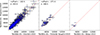 |
Fig. 1. Comparison of Te[N II] measurements used in this work (Brazzini et al. 2024) with three different sets of measurements from the literature. While the auroral line fits in Kreckel et al. (2022) (left) and Rickards Vaught et al. (2024) (center) are both based on the same underlying MUSE data set, different assumptions have been made in the SSP fitting and region boundaries. The Berg et al. (2015) measurements (right) are based on independent long-slit spectroscopy. As there are only five regions in common with Berg et al. (2015), no offset or scatter is calculated in comparison with this sample. |
Finally, we converted these measurements of Te into 12 + log(O/H) using the prescription from Méndez-Delgado et al. (2023a), namely,
![Mathematical equation: $$ \begin{aligned} 12+\mathrm{log(O/H)} = (-1.19\pm 0.14) \times T_{\rm e}([\mathrm{N}\,ii ])/10^4\,\mathrm{K} + (9.68\pm 0.15). \end{aligned} $$](/articles/aa/full_html/2025/11/aa56017-25/aa56017-25-eq2.gif) (1)
(1)
This relation is based on deep longslit spectra of ∼20 Galactic and extragalactic H II regions with temperatures between 8000–13 000 K, spanning approximately 0.6 dex in metallicty. This relation is calibrated to abundance measurements made using OII-recombination lines, which has long been known to produce ∼0.1–0.2 dex higher measurements of 12 + log(O/H) than collisionally excited lines (Wyse 1942; Ferland 2003; Peimbert et al. 2017), such as [O III] λ5007, which are typically used for abundance determinations. This long-standing discrepancy has been the focus of several studies (see Stasińska 2005; García-Rojas & Esteban 2007; Henney & Stasińska 2010; Ferland et al. 2016, and references therein), which attribute it to various physical phenomena, such as the presence of unresolved temperature fluctuations (Méndez-Delgado et al. 2023a). For these reasons, differences between abundances calculated with the Scal strong-line method (empirically calibrated against collisionally excited lines; see Section 2.2) and this prescription are expected to result in an absolute offset.
3. Results
3.1. Te gradients, in individual H II regions and stacks
In Figure 2 we show the measured Te[N II] as a function of radius for each galaxy, comparing the results for individual H II regions with the results obtained from the H II region stacks. Galaxies have been sorted by stellar mass, from low (top) to high (bottom), and all galaxies are shown with matched scales, so it is possible to directly compare the absolute values and slopes across the sample. Higher metallicities are associated with lower temperatures, as metal lines are responsible for cooling, and the overall sample follows the expected mass-metallicity relation (Tremonti et al. 2004), with lower mass systems showing systematically higher Te. While many of the radial gradients are quite flat (as was also seen in Groves et al. 2023), when trends are present, they are typically positive (e.g., NGC 5068, NGC 628, and NGC 1566), which corresponds to the expected negative radial metallicity trends.
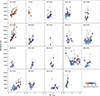 |
Fig. 2. Te[N II] as a function of radius for all 19 galaxies. We compare individual H II regions (S/N > 3 open circles, S/N > 5 filled circles) with measurements from H II region stacks (squares and lines). Points are color-coded by their [N II] λ6583 Luminosity (L[[N II]]). Note: H II regions in NGC 4254 and NGC 4535 do not cover the full disk due to the AO notch filter. Galaxies are ordered from low (top-left) to high (bottom-right) stellar mass. All galaxies are shown with matched scales, so it is possible to directly compare the absolute values and slopes across the sample. |
All points are colored by L([N II]) and when we consider only the individual H II regions, there are a number of galaxies (e.g., NGC 4303, NGC 1566) for which a secondary trend in luminosity is suggested. The less luminous regions (in [N II] λ6583) appear to have higher Te at fixed radius, in excess of the reported uncertainties. Given the faintness of the [N II] λ5755 line, and the fact that higher Te[N II] derives from a higher intrinsic [N II] λ5755/[N II] λ6583 line ratio, this is suspiciously suggestive of simple statistical outliers on the high-end tail of the [N II] λ5755 line flux distribution that bias us towards overestimating Te[N II]. This is supported by the large number of lower 3 < S/N < 5 sources with systematically higher Te measurements. The stacks confirm this, as while they also show a suggestion of a trend for higher Te and lower luminosity, there is significantly less scatter among different luminosity bins at any fixed radial bin (in each galaxy) compared to the individual regions, with temperature differences consistent within the 1σ uncertainties. We revisit the nature of some of the individual high S/N > 5 outliers in Section 3.3, but emphasize the good agreement between all stacked Te measurements and those from the brightest (and hence highest confidence) Te measurements based on individual H II regions.
We note that in addition to the S/N cuts on the [N II] λ5755 line detection, we have also excluded 27 individual regions from our analysis that have reported uncertainties in Te[N II] of more than 500 K. This is ∼3 times higher than the median uncertainty for the sample (146 K) and these 27 regions all have atypically large temperatures. These appear to be a combination of spurious spectral features and unusual emission line stars (see Appendix B).
3.2. Comparison of metallicity gradients
By converting our Te[N II] measurements into a metallicity measurement (see Section 2.4), we can directly compare these ‘direct method’ Te[N II] metallicities with the strong-line Scal metallicities derived for the entire H II region population, in both the individual H II regions and the stacked results. Figure 3 shows this directly for all 19 galaxies and we note that the axes are rescaled for each galaxy to emphasize the comparison between radial trends in the direct method and strong-line prescriptions. Similar comparisons are made for three additional strong-line prescriptions in Appendix C.
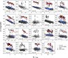 |
Fig. 3. Comparison of metallicity gradients. The Scal values (grey) are compared with individual Te[N II] metallicities (red) and Te[N II] stacked metallicities (black). For context, the subsample of individual regions with Te[N II] detections are highlighted within the Scal measurements in light blue. Linear radial gradients are fit when there are at least five measurements that cover at least 0.5 reff. Note: H II regions in NGC 4254 and NGC 4535 do not cover the full disk due to the AO notch filter. Galaxies are ordered from low (top-left) to high (bottom-right) stellar mass. The axis scalings are not matched between galaxies. |
We included all Te[N II] metallicities with S/N > 3 in our analysis. All radial gradients were fit with outlier removal, using 3σ clipping and three iterations. To ensure robust results, gradients were only fit when at least five data points were available and a range of at least 0.5 reff was covered by the data. All stacked H II region measurements for a given galaxy were considered together to obtain a Te[N II] stack radial gradient for that galaxy.
Qualitatively, we see very good agreements between the slopes in all fits. As explained in Section 2.4, the absolute offset between the Scal and Te[N II] based metallicities is expected, reflecting the abundance discrepancy factor between abundances derived from collisionally excited lines compared to recombination lines. The metallicity of the Te stacks is in good agreement with what is observed in individual H II regions. Our stacking approach also consistently achieves detections towards the galaxy centers where this low-temperature, high-metallicity regime is frequently inaccessible for individual regions without exceptionally deep spectroscopy.
NGC 4254 has sufficiently high systemic velocity that the [N II] λ5755 line detection is severely impacted by the AO filter notch, explaining the poor recovery of Te[N II] metallicities. Other galaxies with poorly sampled Te[N II] metallicities (IC 5332, NGC 1512, NGC 3351) display generally smaller H II region populations and limited radial coverage within the field of view, limiting the effectiveness of our statistical stacking approach.
As the individual H II regions with Te[N II] measurements represent a small fraction of the total H II region population, we isolated and separately fit the Scal metallicities for that exact subset of H II regions (light blue points) to also consider if their Scal gradients accurately reflect the entire population. In general, we see a good agreement, particularly in those galaxies with a large number (> 20) of H II regions with [N II] λ5755 detections. We do note that in some galaxies (e.g., NGC 5068, NGC 628, NGC 7496, NGC 1433), the subsamples with Te[N II] detections are offset towards higher Scal metallicties, but by only a small amount < 0.1 dex. This appears to depend on the calibration adopted (see Appendix C and Figure 13 in Brazzini et al. 2024). This could be related to the effect noted in Kreckel et al. (2019), where more luminous H II regions with higher ionization parameter are correlated with higher offsets from the radial trend (Δ(O/H)), which correspond to localized pockets of enriched material around vigorously star-forming regions that have not become well mixed over > 100 pc scales.
We provide a direct comparison of the metallicity gradient, intercept, and scatter about that gradient for the different linear fits in Figure 4. Both the gradient from the Te[N II] stacks and the individual H II regions follow the 1-to-1 trend compared to the Scal gradient, demonstrating that the Scal metallicities robustly trace the relative changes in metallicity that are recovered from the Te direct method metallicity. The offset in the intercept is well explained by the ADF and corresponds to an absolute underestimate of the Scal metallicities by ∼0.3 dex compared to the recombination line calibrated Te[N II] metallicities.
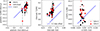 |
Fig. 4. Comparison of the metallicity gradient (left), intercept (center) and scatter (right) between Scal metallicities and the Te[N II] metallicities in individual H II regions (red) and stacks (black). For reference, the 1-to-1 line is shown, as well as a fixed offset of 0.3 dex for the intercept. In the right panel, the scatter is measured using individual regions with S/N > 3 (open) or S/N > 5 (filled). |
One of the surprising characteristics of the Scal metallicity gradients reported by Kreckel et al. (2019) and confirmed in other galaxies (Bresolin et al. 2025) is the very small σ(O/H) of 0.03–0.06 dex routinely measured, which is even smaller when considering σ(O/H) within < kpc scale sub-regions of the galaxies (Kreckel et al. 2020). This is effectively the uncertainty inherent to the prescription and suggests a high level of homogeneity (perhaps due to efficient mixing) in gas-phase abundances. From the Te[N II]-based metallicities of the individual H II regions with S/N > 3, we see slightly higher σ(O/H) (∼0.08 dex), but still almost exclusively measure variations of less than 0.1 dex. We note that the Te[N II]-based metallicities in the stacks show consistently higher levels of homogeneity, with σ(O/H) displaying a good match to the Scal derived values. If the variations in O/H are driven partly by luminosity or azimuthal location, then a possible reason for the stacks to show lower scatter is that we are averaging over the driving variable. However, we also find that σ(O/H) is systematically lower when considering only the high-confidence (S/N > 5) individual detections. As our observed σ(O/H) corresponds to Te variations of ∼700 K, while the typical errors in Te are only ∼150 K, this could also arise if errors in Te[N II] are routinely underestimated, propagating into higher reported values of σ(O/H). The possibility of systematic error underestimation is supported by our measurement of higher than expected scatter when comparing different Te[N II] measurements from the literature for the same set of H II regions (Figure 1), which display a ∼400 K scatter arising from variations in the treatment of the underlying SSP and region size when measuring the auroral line fluxes.
3.3. Metallicity outliers
Given the clear radial gradients in Te[N II] for many of the galaxies and large number of individual H II region detections, it is possible to look specifically at outliers in these distributions to try and understand if these are indicative of significant azimuthal abundance variations. We identified a total of 13 H II regions in nine galaxies with 12 + log(O/H) values based on the Te[N II] measurements that are high-confidence detections (S/N > 5) and are at least 0.1 dex offset below the radial trend, along with two regions at least 0.1 dex offset above the radial trend. Table 2 lists the position of all regions, along with the host galaxy name and region ID as given in Groves et al. (2023) and the Te[N II] metallicity measured for the individual region as well as the median value across all luminosities of the corresponding radial stack.
Locations and metallicities for H II regions with high and low reported Te[N II] metallicities.
These outlier H II regions are generally ∼1σ offset from the radial gradient measured in the individual Te[N II] metallicities (Δ(O/H)). In comparison to the corresponding stack at matched radius, the low-metallicity outliers similarly pronounced, with values 0.2–0.3 dex lower than in the stacks. The high metallicity outliers appear much more consistent with the stacked results (< 0.1 dex offsets).
The H II region outliers in metallicity do not show any strong kinematic signatures distinguishing them from the bulk rotational motion of the disk, as seen in surrounding ionized gas, which might have been expected if these differences were due to external gas accretion effects. Of the regions showing lower metallicities, three are located on spiral arms, three are located in the “disk” environment (typically where no pronounced spiral structure is seen) and seven are in interarm environments. Of the regions with higher metallicities, one is in the “disk” and the other is in an interarm environment. Although these are very small number statistics, the interarm environment appears slightly over-represented (see also Section 4.3), as they contain only ∼35% of all H II regions in these galaxies. Two of the regions with low metallicity in NGC 1385 are located next to each other, with a separation of ∼100 pc.
As it remains challenging to recover Te[N II] measurements for large numbers of individual H II regions, it is useful to examine whether these metallicity outliers are also apparent via their strong-line metallicities. Figure 5 offers of comparison of Δ(O/H) in our 15 outliers, as measured from the Scal prescription and radial gradients, with the full H II region sample. While the two outliers to high metallicity (in red) are also modest outliers in Δ(O/H)Scal, the distribution for the low metallicity outliers is quite flat. This would suggest that if these individual measurements of high Te[N II] are real, then it is not possible to easily identify them from strong-line metallicity prescriptions alone. Inconsistencies when attempting to identify metallicity outliers have also been seen when comparing strong-line methods (see Appendix C in Kreckel et al. 2019). Given large enough sample sizes, by design a small fraction will appear as 3σ outliers in the distribution; however, these inconsistencies (particularly for low metallicity outliers) suggest more stringent criteria should perhaps be applied before interpreting these in the context of pristine gas accretion.
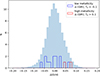 |
Fig. 5. Distribution of Δ(O/H) based on the Scal metallicities for the full H II region sample (filled blue). This is compared with the offsets measured from the strong-line Scal prescription for Te[N II] outliers to low (blue lines) and high (red lines) metallicities. The full H II region sample distribution has been normalized, while the outlier distribution reflects direct counts. |
Finally, we note two extreme outliers (excluded from Table 2 due to large uncertainties in Te[N II]) with reported temperatures that are unphysically large for H II regions (30 000 K and 70 000 K), but convincing [N II] λ5755 detections. However, these appear to be associated with Wolf-Rayet or other emission-line stars (see Appendix B) and a detailed analysis of these sources is beyond the scope of this work.
3.4. Comparison of spiral arm and interarm environments
Our stacking approach enables us to determine the bulk properties of H II regions at fixed radius and luminosity within each of our galaxies. Our sample size is large enough that we can take this a step further and also separate the sample by galactic environment. Many recent studies have identified differences in the metallicity of H II regions on spiral arms compared to interarm environments (Kreckel et al. 2019; Sánchez-Menguiano et al. 2020), although the trends are not strong and are not well reflected in the bulk distribution of metals across the entire environment (Williams et al. 2022).
We split our stacks in radius and luminosity into two further bins, reflecting the arm and interarm environments as defined by Querejeta et al. (2021). Here, we consider only those environments that are outside of the stellar bar (if present) and excluded galaxies where no spiral structure was clearly identified (six galaxies). For stacks where both environments have at least 5 H II regions, we can then directly compare Te[N II] measurements across both environments for the bulk H II region population. Figure 6 shows that both environments agree within ∼500 K across the full range of [N II] luminosities and radii that we cover here. We see no evidence of secondary trends or offsets with either parameter.
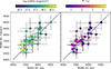 |
Fig. 6. Comparison of Te[N II] measured in stacked arm and interarm environments. We color-code the points by L([N II]) (left) and radius (right), but no evidence is seen for trends or bulk offsets between environments. |
4. Discussion
4.1. Comparison of Scal strong-line and Te[N II] direct method metallicities
Our comparison of direct method Te[N II] metallicities with strong-line Scal metallicities has demonstrated a good agreement between the derived radial gradients (Figure 4), particularly when improving the S/N of the faint [N II] λ5755 auroral line by stacking in radial bins. This provides confirmation that the trends identified within our order of magnitude larger samples of H II regions based on strong-line methods are an accurate reflection of trends in the metallicity. We note that our comparison is limited to the relatively high metallicities (from half-solar to solar) covered by our sample.
A comparison with other strong-line prescriptions is provided in Appendix C. Overall, the metallicity gradient slopes for all prescriptions are broadly correlated with the Te[N II] metallicities, with the O3N2 and N2 prescriptions showing the largest deviations and an overall narrower dynamic range in measured slopes. We observe that the N2S2 (Dopita et al. 2016) calibration behaves similarly to the Scal prescription, which is unsurprising given the strong correlation between metallicities in these two prescriptions (Groves et al. 2023). As the N2S2 metallicities are typically higher, the absolute metallicity values are also in slightly better agreement with our Te[N II] metallicities.
The low (< 0.1 dex) scatter in metallicity that is seen within galaxies relative to their radial gradients, even in the individual Te[N II] metallicity measurements, reflects that a systematic, kpc-scale mixing must be at work to homogenize the metal distribution within galaxy disks. Most of the scatter in the individually detected Te[N II] metallicities is associated with low confidence 3 < S/N < 5 H II regions and is likely to be spurious. Increasing the threshold to include only S/N > 5 regions, our statistics become limited but we do see that the scatter drops to 0.1–0.05 dex, similar to what is found in the Scal metallicities. Again, this provides confirmation that the results obtained on the relative metallicity variations using the Scal metallicities is robust. This high level of homogeneity has been reported in other individual galaxies (e.g., Li et al. 2013; Croxall et al. 2016; Rogers et al. 2022) and with our galaxy sample, we are able to demonstrate that this is likely a general characteristic of spiral galaxies.
The absolute offset between the Te[N II] and Scal metallicities is approximately 0.3 dex across the full range of metallicities probed by our sample. This is due to the ADF, as our prescription for calculating Te[N II] metallicities is calibrated based on recombination lines instead of collisionally excited lines (Méndez-Delgado et al. 2023a). A detailed comparison of strong-line metallicities and Te[N II] measurements for individual regions might reflect differences in unresolved spatial fluctuations in temperature between H II regions, but is beyond the scope of this work. In the calibration of Te[N II] as a metallicity indicator, no secondary dependence on unresolved spatial fluctuations in temperature was seen (Méndez-Delgado et al. 2023a), supporting the case for using this as a robust single-temperature indicator of gas-phase metallicity.
One feature of note in the radial metallicity gradients shown in Figure 3 is that for some galaxies (e.g., NGC 5068, NGC 628, NGC 1433), the individual H II regions with Te[N II] measurements (blue points) are not representative of the full H II region sample when considering their Scal metallicities. They are systematically offset towards higher metallicities by almost 0.1 dex. This effect is not present in all galaxies and does not correlate with absolute metallicity or any other obvious property (e.g., stellar mass, star formation rate, diffuse ionized gas contribution). As the [N II] λ5755 line is faint, these are preferentially the more luminous H II regions in each galaxy and this effect is reminiscent of the correlations reported in Kreckel et al. (2019) for H II regions with a higher ionization parameter, higher Hα luminosity, and younger stellar clusters as being associated with localized enrichment (higher Δ(O/H)). Considering only the Te[N II] metallicities, the smaller number of H II regions and overall larger scatter makes it hard to determine if a similar trend is present. In the H II region stacks, any trends in luminosity are minimized, suggesting that such a trend with luminosity in the Scal metallicities might also be spurious. If so, it would also imply that the radial gradients are even more homogeneous, as Δ(O/H) measured with the Scal prescription gets reduced to < 0.03 dex when considering the subsample of H II regions where [N II] λ5755 is detected.
4.2. Potential use of Te[N II] as a new standard
The use of direct method metallicities, where Te is directly measured in order to constrain ionic abundances, has long been considered a robust method of measuring metallicities in H II regions (Peimbert et al. 2017). Given the ionization structure of H II regions, the most precise approach comes from combining multiple temperatures from multiple ions, constructing two- or three-zone models that can be used to measure both O+ and O++ abundances to compute a total integrated O/H abundance (e.g., Garnett 1992; Bresolin et al. 2009; Berg et al. 2015). When measurements are not available for specific ions, temperature-temperature relations are commonly used to account for information on the missing ionization zones (e.g., Campbell 1988; Berg et al. 2020). However, this detailed approach still relies on assumptions about the nebular conditions (e.g., density; Méndez-Delgado et al. 2023b) and by using multiple ionization zones, it compounds the line flux uncertainties for multiple faint auroral lines.
The canonical approach comes from measuring Te[O III] using the [O III] λ4363 auroral line. However, this line is particularly faint in high metallicity systems, where it can also be blended with [FeII] lines such as λ4360 (Curti et al. 2017; Rogers et al. 2022). In addition, recent works have suggested it may be further biased by shocks arising from localized stellar feedback (Rickards Vaught et al. 2024; Khoram & Belfiore 2025). Constraining O+ requires detection of the [O II] λ7320,7330 auroral lines, which are blanketed by sky lines, and also widely separated from the [O II] λ3727 strong line (also needed to constrain O+); hence, it is sensitive to errors in the extinction correction. In addition, both of these oxygen temperatures rely on emission lines located at blue wavelengths that are not covered by VLT/MUSE, limiting the statistics on these lines until the advent of new instruments such as BlueMUSE (Richard et al. 2019). When these oxygen temperatures are not available, a common alternative is to substitute temperatures from different ions that are expected to populate a similar ionization zone in the nebula. For example, Te[S III] provides an alternative for Te[O III], although it only partly spans the O++ zone and has a strong line and auroral lines that are, again, widely separated in wavelength.
Méndez-Delgado et al. (2023a) demonstrated that Te[N II] provides a remarkably good representation of Te across the entire ionized nebula and it has the added advantage of appearing insensitive to unresolved temperature fluctuations. There is only a modest wavelength separation between the [N II] λ5755 auroral line and [N II] λ6583 strong line, relatively little sky line contamination, and it is very well suited to stacking approaches. In this work, we have explored the use of the sole Te[N II] measurement to infer metallicities across 534 H II regions and 215 stacks. We found good systematic agreement with the results derived from the strong-line Scal prescription.
We highlight two important caveats to our result. First, we have only tested this approach in the high-metallicity regime (8.2 < 12 + log(O/H) < 9.0) and [N II] λ5755 remains challenging to detect in low-metallicity systems. However, the range of metallicities over which Te[N II] provides robust measurements includes virtually all spiral galaxies, highlighting its potential for investigating gradients and mixing in massive galaxies. Second, any detailed dependence of the conversion between Te[N II] and 12 + log(O/H) on the ionization structure of the region (i.e., ionization- vs. density-bounded regions, Wolf-Rayet winds or extreme shocked interior conditions, or blister-like morphology) has not yet been explored. In the case of such realistic complications, the relative contribution of O++ to the total abundance could differ from the reference sample used in Méndez-Delgado et al. (2023a) and a one-zone approach might fail. However, we believe Te[N II] holds significant promise as a new gold standard worthy of more detailed exploration, as it could serve as a foundation for the development of improved strong-line prescriptions.
4.3. The challenge of detecting higher-order or environmental metallicity variations
IFU surveys of nearby galaxies are moving us from radial studies of metallicity, with a small number of H II regions, towards a more comprehensive 2D map of the “metal field”. These higher order patterns in the metal distribution are important to understand, as they hold information on the balance of feedback, accretion, transport, and winds in enriching the ISM (Sharda et al. 2024). The separation of trends by galaxy environment (Ho et al. 2017; Kreckel et al. 2019; Sánchez-Menguiano et al. 2020; Bresolin et al. 2025) mirror some effects seen in some simulations (Grand et al. 2016; Mollá et al. 2019; Spitoni et al. 2019, 2023; Khoperskov et al. 2023; Orr et al. 2023), although sometimes there will be less pronounced (or absent) differences between spiral arm and interarm metallicities (Grasha et al. 2022). Interpolating metallicity measurements between H II regions is also possible by assuming a smooth 2D underlying metal distribution (e.g., Metha et al. 2022); however, thus far this also fails to recover any systematic environmental or other higher-order trends beyond a linear radial gradient (Williams et al. 2022). However, concerns about biases to metallicity diagnostics remain, particularly due to the impact of diffuse ionized gas blended with fainter regions (Poetrodjojo et al. 2019; Pérez-Montero et al. 2023; Lugo-Aranda et al. 2024; González-Díaz et al. 2024).
Ho et al. (2019) demonstrated that metal enrichment along the spiral arm ridge of NGC 1672 is well recovered via azimuthal Te[N II] variations, however, they note that one galaxy remained an outlier (possibly due to its strong bar or well separated spiral arms) in demonstrating such a pronounced environmental trend. As seen in Section 3.3, the extreme outliers in Te[N II] show no strong environmental preference, with only a hint that lower metallicity regions are found more often in the interarm. Also, when stacking all regions at matched luminosity and radius by environment (see Figure 6), we do not see any pronounced difference due to environment alone. As the variation in NGC 1672 was also not recovered by this analysis, we believe this reflects how localized (< 300 pc) these metallicity variations are. This has also been suggested in studies using strong-line metallicities (Kreckel et al. 2020), as they are not easily captured by ∼ kpc scale environmental masks.
We note that our analysis entirely excludes any consideration of the galaxy centers. These environments have shown evidence for unusual stellar abundances (e.g., Sextl et al. 2024), but gas-phase studies remain challenging due to the high level of crowding of H II regions and the potential contribution to line ionization by low-mass stars (given the high stellar density), shocks (from bar-driven gas flows), or AGN excitation.
5. Conclusions
We used PHANGS-MUSE spectroscopy to examine Te[N II] measurements in 534 individual H II regions and 215 stacked regions across 19 nearby galaxies. Using the prescription from Méndez-Delgado et al. (2023a), we converted these values into measurements of the metallicity. After accounting for the instrumental masking of specific wavelength ranges due to the AO system and requiring radial coverage of more than 0.5 reff, we were able to constrain the metallicity gradients in 15 of our target galaxies. We found very good agreement between the radial gradients when compared to strong-line Scal metallicities, but a large 0.3 dex intercept offset due to the abundance discrepancy factor. Our stacking approach considered bins in fixed radius and [N II] λ6583 luminosity and we were able to demonstrate that much of the scatter in Te[N II] metallicities is due to low S/N ∼ 3 detections of [N II] λ5755 in individual regions that introduce biases towards high Te[N II] values. At high S/N > 5, we found very homogeneous gradients in our Te[N II] metallicities across each galaxy (σ(O/H) ∼ 0.1–0.05 dex). From our stacked data, we see consistent results across different luminosity bins and very slight deviations from a linear radial trend, suggesting efficient azimuthal mixing.
Using the individual H II region Te[N II] metallicities, we searched for outliers at the ∼0.1 dex level and identified 13 regions with anomalously low metallicity as well as two regions with anomalously high metallicity. These deviations are not well reflected in the corresponding strong-line metallicities and show no clear correlations with disk kinematics (which might indicate connections with gas flows or external accretion) or environment (e.g., arm vs. interarm). By stacking H II regions separately by arm and interam environments, we did not see any large kpc-scale systematic differences in the abundance either, suggesting that previously identified enrichment along spiral arm ridges must be due to localized processes.
This work tests a temperature-based approach to measuring metallicities that relies only on a single auroral line detection. By demonstrating a good systematic agreement with the well-used Scal strong-line prescription (Pilyugin & Grebel 2016), this serves to cross-validate the two methods for the metallicitiy regime probed by our galaxies. We find the use of Te[N II] demonstrates significant promise for future studies of precise abundance determinations within nearby galaxies.
Acknowledgments
We thank the referee for their careful reading of this work and thoughtful suggestions. KK, EE and FHL gratefully acknowledge funding from the Deutsche Forschungsgemeinschaft (DFG, German Research Foundation) in the form of an Emmy Noether Research Group (grant number KR4598/2-1, PI Kreckel) and the European Research Council’s starting grant ERC StG-101077573 (“ISM-METALS”). SCOG and RSK acknowledge financial support from the European Research Council via the ERC Synergy Grant “ECOGAL” (project ID 855130) and from the German Excellence Strategy via the Heidelberg Cluster of Excellence (EXC 2181 – 390900948) “STRUCTURES”. OE acknowledges funding from the Deutsche Forschungsgemeinschaft (DFG, German Research Foundation) – project-ID 541068876. Table 1 includes distances that were compiled by Anand et al. (2021) from Freedman et al. (2001), Nugent et al. (2006), Jacobs et al. (2009), Kourkchi & Tully (2017), Shaya et al. (2017), Kourkchi et al. (2020) and Scheuermann et al. (2022). Based on observations collected at the European Southern Observatory under ESO programmes 094.C-0623 (PI: Kreckel), 095.C-0473, 098.C-0484 (PI: Blanc), 1100.B-0651 (PHANGS-MUSE; PI: Schinnerer), as well as 094.B-0321 (MAGNUM; PI: Marconi), 099.B-0242, 0100.B-0116, 098.B-0551 (MAD; PI: Carollo) and 097.B-0640 (TIMER; PI: Gadotti). This research has made use of the NASA/IPAC Extragalactic Database (NED) which is operated by the Jet Propulsion Laboratory, California Institute of Technology, under contract with NASA. It also made use of a number of python packages, namely the main ASTROPY package (Astropy Collaboration 2013, 2018, 2022), NUMPY (Harris et al. 2020) and MATPLOTLIB (Hunter 2007).
References
- Anand, G. S., Lee, J. C., Van Dyk, S. D., et al. 2021, MNRAS, 501, 3621 [Google Scholar]
- Andrews, B. H., Weinberg, D. H., Schönrich, R., & Johnson, J. A. 2017, ApJ, 835, 224 [NASA ADS] [CrossRef] [Google Scholar]
- Arsenault, R., Madec, P. Y., Hubin, N., et al. 2008, in Adaptive Optics Systems, SPIE Conf. Ser., 7015, 701524 [NASA ADS] [CrossRef] [Google Scholar]
- Astropy Collaboration (Robitaille, T. P., et al.) 2013, A&A, 558, A33 [NASA ADS] [CrossRef] [EDP Sciences] [Google Scholar]
- Astropy Collaboration (Price-Whelan, A. M., et al.) 2018, AJ, 156, 123 [Google Scholar]
- Astropy Collaboration (Price-Whelan, A. M., et al.) 2022, ApJ, 935, 167 [NASA ADS] [CrossRef] [Google Scholar]
- Bacon, R., Accardo, M., Adjali, L., et al. 2010, in Ground-based and Airborne Instrumentation for Astronomy III, Proc. SPIE, 7735, 773508 [Google Scholar]
- Bacon, R., Conseil, S., Mary, D., et al. 2017, A&A, 608, A1 [NASA ADS] [CrossRef] [EDP Sciences] [Google Scholar]
- Baldwin, J. A., Phillips, M. M., & Terlevich, R. 1981, PASP, 93, 5 [Google Scholar]
- Belfiore, F., Maiolino, R., Tremonti, C., et al. 2017, MNRAS, 469, 151 [Google Scholar]
- Berg, D. A., Skillman, E. D., Croxall, K. V., et al. 2015, ApJ, 806, 16 [NASA ADS] [CrossRef] [Google Scholar]
- Berg, D. A., Pogge, R. W., Skillman, E. D., et al. 2020, ApJ, 893, 96 [NASA ADS] [CrossRef] [Google Scholar]
- Blanc, G. A., Weinzirl, T., Song, M., et al. 2013, AJ, 145, 138 [NASA ADS] [CrossRef] [Google Scholar]
- Brazzini, M., Belfiore, F., Ginolfi, M., et al. 2024, A&A, 691, A173 [NASA ADS] [CrossRef] [EDP Sciences] [Google Scholar]
- Bresolin, F., Gieren, W., Kudritzki, R.-P., et al. 2009, ApJ, 700, 309 [NASA ADS] [CrossRef] [Google Scholar]
- Bresolin, F., Kennicutt, R. C., & Ryan-Weber, E. 2012, ApJ, 750, 122 [NASA ADS] [CrossRef] [Google Scholar]
- Bresolin, F., Fernández-Arenas, D., Rousseau-Nepton, L., et al. 2025, MNRAS, 539, 755 [Google Scholar]
- Bryant, J. J., Owers, M. S., Robotham, A. S. G., et al. 2015, MNRAS, 447, 2857 [Google Scholar]
- Bundy, K., Bershady, M. A., Law, D. R., et al. 2015, ApJ, 798, 7 [Google Scholar]
- Campbell, A. 1988, ApJ, 335, 644 [Google Scholar]
- Cappellari, M. 2017, MNRAS, 466, 798 [Google Scholar]
- Cappellari, M., & Emsellem, E. 2004, PASP, 116, 138 [Google Scholar]
- Chen, Y., Jones, T., Sanders, R. L., et al. 2024, ApJ, submitted [arXiv:2405.18476] [Google Scholar]
- Croxall, K. V., Pogge, R. W., Berg, D. A., Skillman, E. D., & Moustakas, J. 2016, ApJ, 830, 4 [NASA ADS] [CrossRef] [Google Scholar]
- Curti, M., Cresci, G., Mannucci, F., et al. 2017, MNRAS, 465, 1384 [Google Scholar]
- Dalcanton, J. J. 2007, ApJ, 658, 941 [CrossRef] [Google Scholar]
- Dopita, M. A., Kewley, L. J., Sutherland, R. S., & Nicholls, D. C. 2016, Ap&SS, 361, 61 [NASA ADS] [CrossRef] [Google Scholar]
- Emsellem, E., Schinnerer, E., Santoro, F., et al. 2022, A&A, 659, A191 [NASA ADS] [CrossRef] [EDP Sciences] [Google Scholar]
- Esteban, C., García-Rojas, J., Carigi, L., et al. 2014, MNRAS, 443, 624 [NASA ADS] [CrossRef] [Google Scholar]
- Ferland, G. J. 2003, ARA&A, 41, 517 [Google Scholar]
- Ferland, G. J., Henney, W. J., O’Dell, C. R., & Peimbert, M. 2016, Rev. Mex. Astron. Astrofis., 52, 261 [Google Scholar]
- Freedman, W. L., Madore, B. F., Gibson, B. K., et al. 2001, ApJ, 553, 47 [Google Scholar]
- García-Rojas, J., & Esteban, C. 2007, ApJ, 670, 457 [CrossRef] [Google Scholar]
- Garnett, D. R. 1992, AJ, 103, 1330 [NASA ADS] [CrossRef] [Google Scholar]
- González-Díaz, R., Rosales-Ortega, F. F., Galbany, L., et al. 2024, A&A, 687, A20 [NASA ADS] [CrossRef] [EDP Sciences] [Google Scholar]
- Grand, R. J. J., Springel, V., Kawata, D., et al. 2016, MNRAS, 460, L94 [Google Scholar]
- Grasha, K., Chen, Q. H., Battisti, A. J., et al. 2022, ApJ, 929, 118 [NASA ADS] [CrossRef] [Google Scholar]
- Groves, B., Kreckel, K., Santoro, F., et al. 2023, MNRAS, 520, 4902 [Google Scholar]
- Harris, C. R., Millman, K. J., van der Walt, S. J., et al. 2020, Nature, 585, 357 [NASA ADS] [CrossRef] [Google Scholar]
- Henney, W. J., & Stasińska, G. 2010, ApJ, 711, 881 [Google Scholar]
- Ho, I. T. 2019, MNRAS, 485, 3569 [NASA ADS] [CrossRef] [Google Scholar]
- Ho, I. T., Seibert, M., Meidt, S. E., et al. 2017, ApJ, 846, 39 [NASA ADS] [CrossRef] [Google Scholar]
- Ho, I. T., Kreckel, K., Meidt, S. E., et al. 2019, ApJ, 885, L31 [NASA ADS] [CrossRef] [Google Scholar]
- Hunter, J. D. 2007, Comput. Sci. Eng., 9, 90 [NASA ADS] [CrossRef] [Google Scholar]
- Jacobs, B. A., Rizzi, L., Tully, R. B., et al. 2009, AJ, 138, 332 [NASA ADS] [CrossRef] [Google Scholar]
- Johnson, J. W., Weinberg, D. H., Blanc, G. A., et al. 2025, ApJ, 988, 8 [Google Scholar]
- Kauffmann, G., Heckman, T. M., Tremonti, C., et al. 2003, MNRAS, 346, 1055 [Google Scholar]
- Kewley, L. J., Groves, B., Kauffmann, G., & Heckman, T. 2006, MNRAS, 372, 961 [Google Scholar]
- Kewley, L. J., Nicholls, D. C., & Sutherland, R. S. 2019, ARA&A, 57, 511 [Google Scholar]
- Khoperskov, S., Sivkova, E., Saburova, A., et al. 2023, A&A, 671, A56 [NASA ADS] [CrossRef] [EDP Sciences] [Google Scholar]
- Khoram, A. H., & Belfiore, F. 2025, A&A, 693, A150 [NASA ADS] [CrossRef] [EDP Sciences] [Google Scholar]
- Kourkchi, E., & Tully, R. B. 2017, ApJ, 843, 16 [NASA ADS] [CrossRef] [Google Scholar]
- Kourkchi, E., Tully, R. B., Anand, G. S., et al. 2020, ApJ, 896, 3 [NASA ADS] [CrossRef] [Google Scholar]
- Kreckel, K., Groves, B., Bigiel, F., et al. 2017, ApJ, 834, 174 [NASA ADS] [CrossRef] [Google Scholar]
- Kreckel, K., Ho, I. T., Blanc, G. A., et al. 2019, ApJ, 887, 80 [NASA ADS] [CrossRef] [Google Scholar]
- Kreckel, K., Ho, I. T., Blanc, G. A., et al. 2020, MNRAS, 499, 193 [NASA ADS] [CrossRef] [Google Scholar]
- Kreckel, K., Egorov, O. V., Belfiore, F., et al. 2022, A&A, 667, A16 [NASA ADS] [CrossRef] [EDP Sciences] [Google Scholar]
- Lang, P., Meidt, S. E., Rosolowsky, E., et al. 2020, ApJ, 897, 122 [CrossRef] [Google Scholar]
- Leroy, A. K., Schinnerer, E., Hughes, A., et al. 2021, ApJS, 257, 43 [NASA ADS] [CrossRef] [Google Scholar]
- Li, Y., Bresolin, F., & Kennicutt, R. C., Jr. 2013, ApJ, 766, 17 [NASA ADS] [CrossRef] [Google Scholar]
- Lugo-Aranda, A. Z., Sánchez, S. F., Barrera-Ballesteros, J. K., et al. 2024, MNRAS, 528, 6099 [NASA ADS] [CrossRef] [Google Scholar]
- Luridiana, V., Morisset, C., & Shaw, R. A. 2012, in Planetary Nebulae: An Eye to the Future, IAU Symp., 283, 422 [Google Scholar]
- Luridiana, V., Morisset, C., & Shaw, R. A. 2015, A&A, 573, A42 [NASA ADS] [CrossRef] [EDP Sciences] [Google Scholar]
- Maiolino, R., & Mannucci, F. 2019, A&ARv, 27, 3 [Google Scholar]
- Makarov, D., Prugniel, P., Terekhova, N., Courtois, H., & Vauglin, I. 2014, A&A, 570, A13 [NASA ADS] [CrossRef] [EDP Sciences] [Google Scholar]
- Marino, R. A., Rosales-Ortega, F. F., Sánchez, S. F., et al. 2013, A&A, 559, A114 [NASA ADS] [CrossRef] [EDP Sciences] [Google Scholar]
- Méndez-Delgado, J. E., Esteban, C., García-Rojas, J., et al. 2023b, MNRAS, 523, 2952 [CrossRef] [Google Scholar]
- Méndez-Delgado, J. E., Amayo, A., Arellano-Córdova, K. Z., et al. 2022, MNRAS, 510, 4436 [CrossRef] [Google Scholar]
- Méndez-Delgado, J. E., Esteban, C., García-Rojas, J., Kreckel, K., & Peimbert, M. 2023a, Nature, 618, 249 [CrossRef] [Google Scholar]
- Metha, B., Trenti, M., & Chu, T. 2021, MNRAS, 508, 489 [NASA ADS] [CrossRef] [Google Scholar]
- Metha, B., Trenti, M., Chu, T., & Battisti, A. 2022, MNRAS, 514, 4465 [Google Scholar]
- Mollá, M., Díaz, Á. I., Cavichia, O., et al. 2019, MNRAS, 482, 3071 [NASA ADS] [Google Scholar]
- Morisset, C., Charlot, S., Sánchez, S. F., et al. 2025, MNRAS, 538, 1884 [Google Scholar]
- Nugent, P., Sullivan, M., Ellis, R., et al. 2006, ApJ, 645, 841 [CrossRef] [Google Scholar]
- O’Donnell, J. E. 1994, ApJ, 422, 158 [Google Scholar]
- Orr, M. E., Burkhart, B., Wetzel, A., et al. 2023, MNRAS, 521, 3708 [NASA ADS] [CrossRef] [Google Scholar]
- Palla, M., Matteucci, F., Spitoni, E., Vincenzo, F., & Grisoni, V. 2020, MNRAS, 498, 1710 [Google Scholar]
- Palla, M., Magrini, L., Spitoni, E., et al. 2024, A&A, 690, A334 [NASA ADS] [CrossRef] [EDP Sciences] [Google Scholar]
- Peimbert, M. 1967, ApJ, 150, 825 [NASA ADS] [CrossRef] [Google Scholar]
- Peimbert, M., Peimbert, A., & Delgado-Inglada, G. 2017, PASP, 129, 082001 [NASA ADS] [CrossRef] [Google Scholar]
- Pérez-Montero, E., Zinchenko, I. A., Vílchez, J. M., et al. 2023, A&A, 669, A88 [NASA ADS] [CrossRef] [EDP Sciences] [Google Scholar]
- Pessa, I., Schinnerer, E., Sanchez-Blazquez, P., et al. 2023, A&A, 673, A147 [NASA ADS] [CrossRef] [EDP Sciences] [Google Scholar]
- Pilyugin, L. S., & Grebel, E. K. 2016, MNRAS, 457, 3678 [NASA ADS] [CrossRef] [Google Scholar]
- Pilyugin, L. S., Grebel, E. K., & Kniazev, A. Y. 2014, AJ, 147, 131 [NASA ADS] [CrossRef] [Google Scholar]
- Poetrodjojo, H., D’Agostino, J. J., Groves, B., et al. 2019, MNRAS, 487, 79 [Google Scholar]
- Prantzos, N., Abia, C., Chen, T., et al. 2023, MNRAS, 523, 2126 [NASA ADS] [CrossRef] [Google Scholar]
- Querejeta, M., Schinnerer, E., Meidt, S., et al. 2021, A&A, 656, A133 [NASA ADS] [CrossRef] [EDP Sciences] [Google Scholar]
- Richard, J., Bacon, R., Blaizot, J., et al. 2019, ArXiv e-prints [arXiv:1906.01657] [Google Scholar]
- Rickards Vaught, R. J., Sandstrom, K. M., Belfiore, F., et al. 2024, ApJ, 966, 130 [NASA ADS] [CrossRef] [Google Scholar]
- Rogers, N. S. J., Skillman, E. D., Pogge, R. W., et al. 2022, ApJ, 939, 44 [NASA ADS] [CrossRef] [Google Scholar]
- Rosales-Ortega, F. F., Díaz, A. I., Kennicutt, R. C., & Sánchez, S. F. 2011, MNRAS, 415, 2439 [NASA ADS] [CrossRef] [Google Scholar]
- Rousseau-Nepton, L., Martin, R. P., Robert, C., et al. 2019, MNRAS, 489, 5530 [NASA ADS] [CrossRef] [Google Scholar]
- Sánchez, S. F., Kennicutt, R. C., Gil de Paz, A., et al. 2012, A&A, 538, A8 [Google Scholar]
- Sánchez, S. F., Rosales-Ortega, F. F., Iglesias-Páramo, J., et al. 2014, A&A, 563, A49 [CrossRef] [EDP Sciences] [Google Scholar]
- Sánchez-Menguiano, L., Sánchez, S. F., Pérez, I., et al. 2016, A&A, 587, A70 [NASA ADS] [CrossRef] [EDP Sciences] [Google Scholar]
- Sánchez-Menguiano, L., Sánchez, S. F., Pérez, I., et al. 2018, A&A, 609, A119 [NASA ADS] [CrossRef] [EDP Sciences] [Google Scholar]
- Sánchez-Menguiano, L., Sánchez, S. F., Pérez, I., et al. 2020, MNRAS, 492, 4149 [CrossRef] [Google Scholar]
- Santoro, F., Kreckel, K., Belfiore, F., et al. 2022, A&A, 658, A188 [NASA ADS] [CrossRef] [EDP Sciences] [Google Scholar]
- Scheuermann, F., Kreckel, K., Anand, G. S., et al. 2022, MNRAS, 511, 6087 [NASA ADS] [CrossRef] [Google Scholar]
- Sextl, E., Kudritzki, R.-P., Burkert, A., et al. 2024, ApJ, 960, 83 [Google Scholar]
- Sharda, P., Ginzburg, O., Krumholz, M. R., et al. 2024, MNRAS, 528, 2232 [NASA ADS] [CrossRef] [Google Scholar]
- Shaya, E. J., Tully, R. B., Hoffman, Y., & Pomarède, D. 2017, ApJ, 850, 207 [NASA ADS] [CrossRef] [Google Scholar]
- Skillman, E. D., Berg, D. A., Pogge, R. W., et al. 2020, ApJ, 894, 138 [NASA ADS] [CrossRef] [Google Scholar]
- Spitoni, E., Cescutti, G., Minchev, I., et al. 2019, A&A, 628, A38 [NASA ADS] [CrossRef] [EDP Sciences] [Google Scholar]
- Spitoni, E., Cescutti, G., Recio-Blanco, A., et al. 2023, A&A, 680, A85 [NASA ADS] [CrossRef] [EDP Sciences] [Google Scholar]
- Stasińska, G. 2005, A&A, 434, 507 [NASA ADS] [CrossRef] [EDP Sciences] [Google Scholar]
- Ströbele, S., La Penna, P., Arsenault, R., et al. 2012, in Adaptive Optics Systems III, SPIE Conf. Ser., 8447, 844737 [CrossRef] [Google Scholar]
- Toribio San Cipriano, L., García-Rojas, J., Esteban, C., Bresolin, F., & Peimbert, M. 2016, MNRAS, 458, 1866 [NASA ADS] [CrossRef] [Google Scholar]
- Tremonti, C. A., Heckman, T. M., Kauffmann, G., et al. 2004, ApJ, 613, 898 [Google Scholar]
- Vazdekis, A., Koleva, M., Ricciardelli, E., Röck, B., & Falcón-Barroso, J. 2016, MNRAS, 463, 3409 [Google Scholar]
- Williams, T. G., Kreckel, K., Belfiore, F., et al. 2022, MNRAS, 509, 1303 [Google Scholar]
- Wyse, A. B. 1942, ApJ, 95, 356 [NASA ADS] [CrossRef] [Google Scholar]
Appendix A: Example stacked spectra
In Section 2.3, we describe our technique for stacking H II regions in bins of luminosity and radius to improve our detection of the [N II]λ5755 auroral line. In Fig. A.1 we provide examples of our spectral stacks for a series of luminosity bins in NGC 628, at a fixed radius of 1 reff. Even for large samples of 100-200 H II regions, we generally do not recover auroral line detections at L([N II]) < 1037 erg s−1, however clear improvements are seen in the brighter luminosity bins.
Appendix B: Emission-line stars
In exploring our Te[N II] catalog (Groves et al. 2023) for outliers, we identified two sources (NGC 2835, region ID #16 and NGC 628, region ID #179) with extremely high Te > 20,000 K, large reported errors (above 500 K) but clear [N II]λ5755 line detections. Taken at face value, these objects have Te measurements of 70,000 K and 31,000 K. Reducing this to something closer to 10,000 K would require an overestimation of the [N II]λ5755 line flux by a factor of five. The spectra for the two robust detections, including the SSP model and single Gaussian fits to emission lines, are shown in Fig. B.1. Interestingly, both have very broad wings in the Hα emission, which are not well fit using a single Gaussian, though the [N II]λ6583 line fluxes appear only modestly affected by the blending.
This unusual broad Hα feature makes it likely these objects arise from some type of emission line star, possibly a Wolf-Rayet star. We note that the object identified in NGC 628, region ID#179 is already reported in Kreckel et al. (2017) and labeled as a possible emission line star. In the environments surrounding Wolf-Rayet stars, the wind ejection of enriched material may result in clumps of nitrogen-enriched material with high densities (ne > 10, 000 cm−3). If a low electron density is assumed (as would be suggested by the observed integrated [S II] line ratio), this may result in a subsequent overestimation of the corresponding electron temperature for these sources.
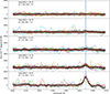 |
Fig. B.1. Example of the resulting stacked spectra in bins of log(L[N II]) = 0.5 at a radius of 1 reff within the galaxy NGC 628, with all spectra shifted to their rest wavelength based on their Hα velocity. Individual H II region spectra are shown in color, the mean stacked spectrum is shown in black, and the fit is shown in red. This wavelength range focuses on the [N II]λ5755 line, marked with a blue dashed line. The luminosity bin, number of individual H II regions included, and resulting S/N of the fit are shown in the upper left corner of each plot. |
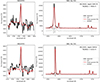 |
Fig. B.2. Two extreme outliers identified in our sample, with reported electron temperatures of 70,000 K (top, NGC 628 region ID #179) and 30,000 K (bottom, NGC 2835 region ID #16). For each object we show the observed spectrum (black) the SSP model (grey), single Gaussian line fits (red) and fit residuals (dashed). The [N II]λ5755 line (left panels) is significantly detected and well fit. Both objects exhibit extremely broad Hα wings (right panels). |
All other extreme outliers encountered in our catalog are associated with high stellar continuum flux, such that the auroral line detection is likely an artifact of the stellar subtraction procedure.
Appendix C: Alternative strong-line calibrations
In Section 3.1 and Fig. 3, we show a comparison of the strong-line S-calibration metallicities with our Te-based measurements. Here, we repeat this for alternative metallicity prescriptions, to facilitate a qualitative comparison of the behavior of each compared to the Te-based metallicities.
Figure C.1 uses the Dopita et al. (2016) calibration based on N2S2. Figure C.2 uses the Marino et al. (2013) calibration of the O3N2 diagnostic, and Fig. C.3 uses their N2 diagnostic calibration.
A direct comparison of the slopes derived for each calibration compared to the Te[N II] metallicity gradients is shown in Figure C.4. While all show clear correlations, O3N2 and N2 show a smaller dynamic range in metallicity gradients.
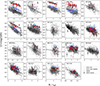 |
Fig. C.1. Comparison of the our Te-based metallicities with strong-line metallicities in our galaxy sample, as a function of radius. Here, we use the N2S2 Dopita et al. (2016) strong-line calibration. The N2S2 values (grey) are compared with individual Te[N II] metallicities (red) and Te[N II] stacked metallicities (black). For context, the subsample of individual regions with Te[N II] detections are highlighted within the N2S2 measurements in light blue. Linear radial gradients are fit when there are at least 5 measurements that cover at least 0.5 reff. Galaxies are ordered from low (top) to high (bottom) stellar mass, and axis scalings are not matched between galaxies. |
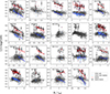 |
Fig. C.2. Comparison of the our Te-based metallicities with strong-line metallicities in our galaxy sample, as a function of radius. Here, we use the O3N2 Marino et al. (2013) strong-line calibration. The O3N2 values (grey) are compared with individual Te[N II] metallicities (red) and Te[N II] stacked metallicities (black). For context, the subsample of individual regions with Te[N II] detections are highlighted within the O3N2 measurements in light blue. Linear radial gradients are fit when there are at least five measurements that cover at least 0.5 reff. Galaxies are ordered from low (top) to high (bottom) stellar mass, and axis scalings are not matched between galaxies. |
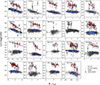 |
Fig. C.3. Comparison of the our Te-based metallicities with strong-line metallicities in our galaxy sample, as a function of radius. Here, we use the N2 Marino et al. (2013) strong-line calibration. The N2 values (grey) are compared with individual Te[N II] metallicities (red) and Te[N II] stacked metallicities (black). For context, the subsample of individual regions with Te[N II] detections are highlighted within the N2 measurements in light blue. Linear radial gradients are fit when there are at least 5 measurements that cover at least 0.5 reff. Galaxies are ordered from low (top) to high (bottom) stellar mass, and axis scalings are not matched between galaxies. |
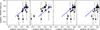 |
Fig. C.4. Comparison of the metallicity gradient slopes from our Te-based metallicities with different strong-line calibrations, including the Scal (left), N2S2 (center left), O3N2 (center right), and N2 (right). The blue one-to-one line is shown for reference. |
All Tables
Locations and metallicities for H II regions with high and low reported Te[N II] metallicities.
All Figures
|
Fig. 1. Comparison of Te[N II] measurements used in this work (Brazzini et al. 2024) with three different sets of measurements from the literature. While the auroral line fits in Kreckel et al. (2022) (left) and Rickards Vaught et al. (2024) (center) are both based on the same underlying MUSE data set, different assumptions have been made in the SSP fitting and region boundaries. The Berg et al. (2015) measurements (right) are based on independent long-slit spectroscopy. As there are only five regions in common with Berg et al. (2015), no offset or scatter is calculated in comparison with this sample. |
| In the text | |
|
Fig. 2. Te[N II] as a function of radius for all 19 galaxies. We compare individual H II regions (S/N > 3 open circles, S/N > 5 filled circles) with measurements from H II region stacks (squares and lines). Points are color-coded by their [N II] λ6583 Luminosity (L[[N II]]). Note: H II regions in NGC 4254 and NGC 4535 do not cover the full disk due to the AO notch filter. Galaxies are ordered from low (top-left) to high (bottom-right) stellar mass. All galaxies are shown with matched scales, so it is possible to directly compare the absolute values and slopes across the sample. |
| In the text | |
|
Fig. 3. Comparison of metallicity gradients. The Scal values (grey) are compared with individual Te[N II] metallicities (red) and Te[N II] stacked metallicities (black). For context, the subsample of individual regions with Te[N II] detections are highlighted within the Scal measurements in light blue. Linear radial gradients are fit when there are at least five measurements that cover at least 0.5 reff. Note: H II regions in NGC 4254 and NGC 4535 do not cover the full disk due to the AO notch filter. Galaxies are ordered from low (top-left) to high (bottom-right) stellar mass. The axis scalings are not matched between galaxies. |
| In the text | |
|
Fig. 4. Comparison of the metallicity gradient (left), intercept (center) and scatter (right) between Scal metallicities and the Te[N II] metallicities in individual H II regions (red) and stacks (black). For reference, the 1-to-1 line is shown, as well as a fixed offset of 0.3 dex for the intercept. In the right panel, the scatter is measured using individual regions with S/N > 3 (open) or S/N > 5 (filled). |
| In the text | |
|
Fig. 5. Distribution of Δ(O/H) based on the Scal metallicities for the full H II region sample (filled blue). This is compared with the offsets measured from the strong-line Scal prescription for Te[N II] outliers to low (blue lines) and high (red lines) metallicities. The full H II region sample distribution has been normalized, while the outlier distribution reflects direct counts. |
| In the text | |
|
Fig. 6. Comparison of Te[N II] measured in stacked arm and interarm environments. We color-code the points by L([N II]) (left) and radius (right), but no evidence is seen for trends or bulk offsets between environments. |
| In the text | |
|
Fig. B.1. Example of the resulting stacked spectra in bins of log(L[N II]) = 0.5 at a radius of 1 reff within the galaxy NGC 628, with all spectra shifted to their rest wavelength based on their Hα velocity. Individual H II region spectra are shown in color, the mean stacked spectrum is shown in black, and the fit is shown in red. This wavelength range focuses on the [N II]λ5755 line, marked with a blue dashed line. The luminosity bin, number of individual H II regions included, and resulting S/N of the fit are shown in the upper left corner of each plot. |
| In the text | |
|
Fig. B.2. Two extreme outliers identified in our sample, with reported electron temperatures of 70,000 K (top, NGC 628 region ID #179) and 30,000 K (bottom, NGC 2835 region ID #16). For each object we show the observed spectrum (black) the SSP model (grey), single Gaussian line fits (red) and fit residuals (dashed). The [N II]λ5755 line (left panels) is significantly detected and well fit. Both objects exhibit extremely broad Hα wings (right panels). |
| In the text | |
|
Fig. C.1. Comparison of the our Te-based metallicities with strong-line metallicities in our galaxy sample, as a function of radius. Here, we use the N2S2 Dopita et al. (2016) strong-line calibration. The N2S2 values (grey) are compared with individual Te[N II] metallicities (red) and Te[N II] stacked metallicities (black). For context, the subsample of individual regions with Te[N II] detections are highlighted within the N2S2 measurements in light blue. Linear radial gradients are fit when there are at least 5 measurements that cover at least 0.5 reff. Galaxies are ordered from low (top) to high (bottom) stellar mass, and axis scalings are not matched between galaxies. |
| In the text | |
|
Fig. C.2. Comparison of the our Te-based metallicities with strong-line metallicities in our galaxy sample, as a function of radius. Here, we use the O3N2 Marino et al. (2013) strong-line calibration. The O3N2 values (grey) are compared with individual Te[N II] metallicities (red) and Te[N II] stacked metallicities (black). For context, the subsample of individual regions with Te[N II] detections are highlighted within the O3N2 measurements in light blue. Linear radial gradients are fit when there are at least five measurements that cover at least 0.5 reff. Galaxies are ordered from low (top) to high (bottom) stellar mass, and axis scalings are not matched between galaxies. |
| In the text | |
|
Fig. C.3. Comparison of the our Te-based metallicities with strong-line metallicities in our galaxy sample, as a function of radius. Here, we use the N2 Marino et al. (2013) strong-line calibration. The N2 values (grey) are compared with individual Te[N II] metallicities (red) and Te[N II] stacked metallicities (black). For context, the subsample of individual regions with Te[N II] detections are highlighted within the N2 measurements in light blue. Linear radial gradients are fit when there are at least 5 measurements that cover at least 0.5 reff. Galaxies are ordered from low (top) to high (bottom) stellar mass, and axis scalings are not matched between galaxies. |
| In the text | |
|
Fig. C.4. Comparison of the metallicity gradient slopes from our Te-based metallicities with different strong-line calibrations, including the Scal (left), N2S2 (center left), O3N2 (center right), and N2 (right). The blue one-to-one line is shown for reference. |
| In the text | |
Current usage metrics show cumulative count of Article Views (full-text article views including HTML views, PDF and ePub downloads, according to the available data) and Abstracts Views on Vision4Press platform.
Data correspond to usage on the plateform after 2015. The current usage metrics is available 48-96 hours after online publication and is updated daily on week days.
Initial download of the metrics may take a while.