| Issue |
A&A
Volume 703, November 2025
|
|
|---|---|---|
| Article Number | A305 | |
| Number of page(s) | 7 | |
| Section | Extragalactic astronomy | |
| DOI | https://doi.org/10.1051/0004-6361/202556191 | |
| Published online | 25 November 2025 | |
Discovery of the asymmetric effect in the response of photoionization gas
1
Department of Astronomy, University of Science and Technology of China, Hefei 230026, China
2
School of Astronomy and Space Science, University of Science and Technology of China, Hefei, Anhui 230026, China
⋆ Corresponding author: mailto:This email address is being protected from spambots. You need JavaScript enabled to view it.
Received:
1
July
2025
Accepted:
7
October
2025
Context. Ionized gas is ubiquitous in the Universe and plays a central role in tracing the cosmic evolution and probing plasma physics under extreme conditions. Of the various ionizing sources, quasars (powered by supermassive black holes) are important contributors to the reionization of the universe. The variability of the quasar radiation provides a valuable opportunity to study the photoionization response of interstellar and intergalactic gas.
Aims. We investigate the physical origin of the asymmetric response of ionized gas to the variable quasar radiation, particularly as observed in broad absorption line (BAL) systems. We also place constraints on the gas density and spatial scale of the BAL outflows based on this asymmetry.
Methods. We conducted time-dependent photoionization simulations focusing on C IV to quantify the response timescales in different ionization states. Analytical estimates were also used to relate the response asymmetry to the gas density.
Results. We find that over 70% of BAL gas in quasar host galaxies exhibit a negative response to variations in the quasar radiation, indicating a strong asymmetry in the behavior of ionized gas. Our simulations show that this asymmetry arises from shorter response timescales at higher ionization states. For typical observational cadences (> 1 day), the observed asymmetry requires that at least 40% of the BAL gas has a density below nH = 106 cm−3, which is consistent with most measured BAL gas densities. This is in contrast to the typical density of accretion disk winds (nH > 108 cm−3), which suggests that BAL outflows either evolve significantly as they propagate outward or originate from larger-scale regions, such as the dusty torus.
Conclusions. We uncovered a fundamental asymmetry in the response of ionized gas: The response timescales of high-ionization states are shorter than those of low-ionization states. The role of the asymmetric response effects thus offers new constraints on the physical origin and structure of quasar outflows.
Key words: line: formation / ISM: jets and outflows / galaxies: active / galaxies: ISM
© The Authors 2025
 Open Access article, published by EDP Sciences, under the terms of the Creative Commons Attribution License (https://creativecommons.org/licenses/by/4.0), which permits unrestricted use, distribution, and reproduction in any medium, provided the original work is properly cited.
This article is published in open access under the Subscribe to Open model. This email address is being protected from spambots. You need JavaScript enabled to view it. to support open access publication.
1. Introduction
Ionized gas is prevalent in the universe at high redshifts (z > 1100) and after the cosmic reionization epoch with z < 6 (Barkana & Loeb 2001; Kriss et al. 2001; Zheng et al. 2004; Fan et al. 2006; Tilvi et al. 2020; Yung et al. 2020). Astrophysical plasma is found in entities such as the interstellar medium (ISM) and intergalactic medium (IGM). It serves as a valuable tool for exploring the evolutionary processes of the universe and celestial bodies. Simultaneously, cosmic celestial bodies provide an ideal laboratory for studying the principles of plasma physics in extreme situations such as extremely high temperatures or low densities. Quasars are a class of high-luminosity active galactic nuclei (AGNs), fueled by the accretion disk of supermassive black holes (SMBHs), stand out as the most luminous and persistent celestial objects in the universe. Their redshift frontier extends to approximately z ∼ 7.6 (Wang et al. 2021). Quasars are thought to play crucial roles in cosmic reionization (Jakobsen et al. 1994; Loeb & Barkana 2001; Fan et al. 2023) and in the evolution of galaxies (Fabian 2012; Kormendy & Ho 2013; Veilleux et al. 2020), through the intense ionizing radiation and enormous energy that is released outward.
The radiation of a quasar typically displays aperiodic variabilities that are often described by the damped random walk (DRW) model (Kelly et al. 2009). The variability of the quasar radiation provides a useful probe of the response of ionized gas and of its density and spatial distribution (Nicastro et al. 1999; Krongold et al. 2007; Kaastra et al. 2012; García et al. 2013; He et al. 2014, 2015, 2019; He et al. 2022; Rogantini et al. 2022; Sadaula et al. 2023; Sadaula & Kallman 2024). The ionization state of a gaseous outflow needs a period of time to respond to changes in the ionizing continuum (the recombination timescale t*; e.g., Krolik & Kriss 1995). Therefore, the gas ionization state is connected to the intensity of the ionizing continuum over t*. At this point, the function of the t* is to induce a smoothing effect. As illustrated in Fig. 1, the population density of a specific ion in the plasma initially increases to a peak and then decreases with the rise in ionization level. Based on the peak position, it can therefore be classified into two stages: the low-ionization state, and the high-ionization state. In the low-ionization state, the ion column density increases with increasing ionizing luminosity, indicating a positive correlation between the two that is referred to as a positive response. Conversely, in the high-ionization state, the ion column density decreases as the ionizing luminosity increases, which shows a negative correlation between the two that is known as a negative response.
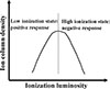 |
Fig. 1. Schematic diagram of the variation in the ion column density with ionization luminosity. The column density of a specific ion in the plasma initially increases to a peak and then decreases with the rise in ionization level. The vertical dashed line represents the peak position. |
Some studies (e.g., Wang et al. 2015; He et al. 2017) used the large sample from the Sloan Digital Sky Survey (SDSS) and revealed that over 70% of the Si IV (ionization energy 45.1 ev), C IV (64.5 ev), N V (97.9 ev) broad absorption lines (BALs) exhibit a negative response. In other words, the majority of gases with variable BALs are in a highly ionized state. This caused some speculation, for instance, whether this negative response persists for ions with higher ionization energies, such as O VI (138.1 ev), or highly ionized iron (> 1 kev), and if it arises because most BAL gases are in a highly ionized state, or if some physical asymmetry in the plasma causes highly ionized ions to respond more easily to variations in the radiation source.
We explore the asymmetry of the plasma response to radiation sources for low- and high-ionization states. Section 2 presents a comprehensive analysis of the asymmetry in the plasma response timescales. In Section 3 we apply this asymmetry to C IV using a photoionization simulation. The final section provides a summary.
2. The asymmetric effect of the response timescale
Studies of BALs in quasar spectra have shown that ions such as N4+, C3+, and Si3+ in the gas surrounding quasars are primarily governed by photoionization (e.g., Wang et al. 2015; He et al. 2017, 2022; Lu et al. 2018; Hemler et al. 2019; Vivek 2019; Zhao et al. 2021). Therefore, we focused on gases that are dominated by photoionization. We provide an overview of the derivation process for the precise recombination timescale of the photoionization gas in the literature (e.g., Arav et al. 2012; Netzer 2013). The population density of of a given element in ionization stage i is represented by
where the ionization rate per particle is Ii, and the recombination rate per particle from the ionization stage i+1 to i is Ri. We exclusively focused on the photoionization processes and omitted collisional ionization from our analysis. Equation (1) forms a set of n+1 coupled differential equations for an element with n electrons and n+1 ions. In the state of photoionization equilibrium, that is, when dni/dt = 0, these reduce to n equations of the form

This implies that the increase of stage i by recombination from stage i+1 must be balanced by the decrease of stage i by ionization to stage i+1. For an optically thin gas at a distance r from the radiation source with a spectral luminosity Lν at a frequency ν, the ionization rate (s−1) per ion of stage i is given by

Γi is the integral ionization cross-section rate (cm2 s−1) over the photons with frequency ν > νi,
where h is Planck’s constant, and σν is the ionization cross section for photons of energy hν. The σν for different atoms and ions can be obtained from the fitting formula in Equation (1) and Table (1) in Verner et al. (1996). The recombination rate per particle is given by

where the recombination coefficient αi depends on the electron temperature T (Osterbrock & Ferland 2006).
We assumed that an absorber in photoionization equilibrium experiences a sudden change in the incident ionizing flux such that Ii(t > 0) = (1 + f)Ii(t = 0), where −1 ≤ f ≤ +∞. At this moment, the column densities of adjacent valence ions and recombination coefficients have not yet had the opportunity to adjust in response to the sudden change in the incident photon flux, that is, dni = dni − 1 = dni + 1 = dRi = dRi − 1 = 0. Therefore, based on Equations (1) and (2), the evolution of ni can be written as
Then, the response timescale for change in the ionic fraction is
![$$ \begin{aligned} t_i^*=\frac{\mathrm{d} t}{\mathrm{d} \ln n_i}&=\left[f \alpha _{i} n_{e}\left(\frac{\alpha _{i-1}}{\alpha _{i}}-\frac{n_{i+1}}{n_{i}}\right)\right]^{-1},\ \mathrm{or} \end{aligned} $$](/articles/aa/full_html/2025/11/aa56191-25/aa56191-25-eq7.gif)
![$$ \begin{aligned}&= \left[f (n_{e}\alpha _{i-1}-I_i)\right]^{-1}. \end{aligned} $$](/articles/aa/full_html/2025/11/aa56191-25/aa56191-25-eq8.gif)
The response timescale here is the e-folding time, that is, the time required for the initial column density to increase e times or decrease to 1/e based on the initial rate of change. The e-folding time is directly proportional to the equilibrium time, with only one additional factor f compared to the equilibrium time. Strictly speaking, the above equations are valid only at the initial moment. Nevertheless, they remain highly informative because they reveal the sign of the response (positive or negative) and the response timescale over which the ion concentration evolves. As shown in Fig. 2, the regime can be divided into high- and low-ionization states according to the position of ni + 1/ni = αi − 1/αi or Ii = neαi − 1. The boundary between the low- and high-ionization states and the boundary defined by the peak column density are misaligned. This misalignment gives rise to a novel mixed-response effect (see He et al. 2025). This effect only arises near the intermediate boundary, however, and does not affect the asymmetry between the extremely low- and extremely high-ionization states that are the focus of this work. When the gas is in a sufficiently low ionization state, that is, ni + 1/ni ≪ αi − 1/αi or Ii ≪ neαi − 1, the response timescale is ti* = 1/(fneαi − 1). When the gas is in a sufficiently high ionization state, in contrast, that is, ni + 1/ni ≫ αi − 1/αi or Ii ≫ neαi − 1, the response timescale is  = −r2/(fΓi). Clearly, this timescale is asymmetrical for low- and high-ionization states. In the low-ionization state, the response timescale is dominated by the recombination coefficient (i.e., the so-called recombination timescale), and in the high-ionization state, it is dominated by the ionization rate. In a highly ionized state, t* is shorter, that is, when the radiation source flux changes, the time required to return to gas ionization equilibrium is shorter. The preceding discussion is based on a theoretical analysis. In the next section, we test these conclusions through time-dependent photoionization simulations.
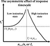 |
Fig. 2. Schematic diagram of the asymmetric effect of ion response timescale. The vertical dashed line is the boundary between the low ionized state and the high ionized state. In a sufficiently low ionization state, i.e., ni + 1/ni ≪ αi − 1/αi or Ii ≪ neαi − 1, the response timescale is ti* = 1/(fneαi − 1). In a sufficiently high ionization state, in contrast, i.e., ni + 1/ni ≫ αi − 1/αi or Ii ≫ neαi − 1, the response timescale is |
3. Photoionization simulations for carbon ions
In this section, we outline the detailed parameter settings of our photoionization simulations. Then, we use the ion C3+ as a case study to illustrate the asymmetric response.
We adopted typical parameters for BAL gas in quasars, with two gas densities of nH = 104, 106 cm−3 and a column density of NH = 1020 cm−2. Using CLOUDY simulations (Ferland et al. 2017), we computed models for a wide ionization parameter range, −4 < log10U < 2, with a step size of Δlog10U = 0.1. The spectral energy distribution (SED) of the ionizing radiation source was UV-SOFT (Dunn et al. 2010), which is representative of high-luminosity radio-quiet quasars. A standard solar metallicity was adopted for the gas. The ionization parameter was defined as
where
is the source emission rate of hydrogen-ionizing photons, and hν0 = 13.6 eV is the ionization potential of H0 for ionization out of the 1-s ground state. c is the speed of light in vacuum. As shown in Fig. 3, the column densities of carbon ions first increase and then decrease with the ionization parameter. Based on the peak position of each ion, we divide dthe parameter space into corresponding low- and high-ionization intervals. Moreover, as the ionization energy of the ions increased, the transition boundary between the low- and high-ionization states systematically shifted toward higher-ionization parameters.
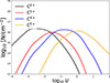 |
Fig. 3. Nonmonotonic dependence of the carbon ion column densities on the ionization parameter. The column densities of carbon ions first increase and then decrease with the ionization parameter. |
3.1. The asymmetrical response timescales of C IV
According the Equation (7), the expression for the response timescale of C IV (i.e., C3+) is
![$$ \begin{aligned} t^{*}_{\mathrm{C}\,{iv }}= \left[f \alpha _{\mathrm{C}\,{iv }} n_{e}\left(\frac{\alpha _{\mathrm{C}\,{iii }}}{\alpha _{\mathrm{C}\,{iv }}}-\frac{n_{\mathrm{C}\,{v }}}{n_{\mathrm{C}\,{iv }}}\right)\right]^{-1}. \end{aligned} $$](/articles/aa/full_html/2025/11/aa56191-25/aa56191-25-eq13.gif)
In our calculation, we adopted a typical variation amplitude f = 1 in the ionizing radiation band of AGN (mainly extreme ultraviolet). As shown in Fig. 4, the curves of the recombination coefficients of C III and C IV and the ratio of the population density nC V/nC IV as a function of ionization parameters U can be obtained from the photoionization simulations using Cloudy c17 (Ferland et al. 2017). As shown in Fig. 5, we calculated the value of the t∗(C IV) at log10 U from –4 to 2 for nH = 104 cm−3 and 106 cm−3, respectively, based on the curves of the recombination coefficients of C III and C IV and on the ratio of the population density nC V/nC IV. Consistent with theoretical expectations, the response timescales of high-ionization states are markedly shorter than those in low-ionization states. In the low-ionization state, t∗(C IV) is about 100 and 1 days for nH = 104 cm−3 and 106 cm−3, respectively. In the high-ionization state, such as log10U = 0, t∗(C IV) is lower than 10 and 0.1 days for nH = 104 cm−3 and 106 cm−3, respectively.
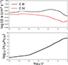 |
Fig. 4. Recombination coefficients and ion concentrations predicted by equilibrium-state photoionization simulations. The recombination coefficients of C III and C IV, as well as the population density ratio nC V/nC IV under different ionization parameters, were obtained from equilibrium photoionization simulations using Cloudy version c17 (Ferland et al. 2017). |
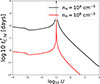 |
Fig. 5. Response timescale of C IV under different ionization parameters. The black and red curves correspond to gas densities of 104 cm−3 and 106 cm−3, respectively. The timescale exhibits strong asymmetry: the response timescale of highly ionized states is significantly shorter than that of low-ionized states. If the observational time interval falls within 1–1000 days, this asymmetry would not be detectable for gas at a density of 106 cm−3, but it would be observable for gas with a density of 104 cm−3. |
3.2. Time-dependent photoionization simulations
Although the response timescales predicted by equilibrium-state photoionization simulations in the previous section are consistent with the theoretical analysis, the determination of whether low- and high-ionization states exhibit positive or negative responses still requires verification through time-dependent simulations. Moreover, the response timescale given by Equation (11) is generally applicable only at the initial moment of a radiation change. Whether it can represent the characteristic timescale of the entire response process also needs to be examined through time-dependent simulations.
We used the time command in CLOUDY to perform time-dependent simulations. As shown in Fig. 6, we selected two ionization parameters, log10U = −3 and log10U = 0, to represent low- and high-ionization states, respectively. These two cases exhibit positive and negative responses, respectively. According to Equation (11), the response timescales for log10U = −3 and log10U = 0 are 48.3 days and 5.5 days, respectively, indicating that the C IV concentration changes more rapidly at log10U = 0. As shown in Fig. 6, the results are fully consistent with the time-dependent simulations, which indicate that the C IV concentration evolves more slowly at log10U = −3 than at log10U = 0. At the initial moment, the rate of change predicted by Equation (11) coincides with the tangent to the simulation curve, further validating the theoretical analysis. The response timescale of photoionized gases in this work ignores processes such as heating and cooling and radiative transfer (e.g., Sadaula et al. 2023). Therefore, it is a simplification of the actual situation. The predicted rate of change matches the Cloudy simulations well, however, indicating that processes such as heating and cooling and radiative transfer are indeed unimportant.
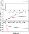 |
Fig. 6. Time-dependent photoionization simulations for the case of the light curve of the step function. At t = 0, the radiation flux is suddenly increased from 1 to 2, corresponding to a change amplitude of f = 1. This leads to a positive response in the low-ionization state (log10U = −3) and a negative response in the high-ionization state (log10U = 0). The dashed red lines represent the response timescales at the initial time predicted by Equation (11). The response timescales for log10U = −3 and log10U = 0 are 48.3 days and 5.5 days, respectively, indicating that the C IV concentration evolves more rapidly at higher ionization (log10U = 0). |
The above analysis is based on the simplified assumption that the light curve behaves as a step function. To further examine the response of high- and low-ionization states in AGN light curves, we adopted the damped random walk (DRW) model (Kelly et al. 2009; Kozłowski et al. 2009). For a representative high-luminosity quasar, we assumed a black hole mass of MBH = 109 M⊙, a characteristic timescale of τ = 30 days, and a structure function defined as SF(Δt) = SF∞(1 − e−|Δt|/τ)1/2 with an asymptotic amplitude of SF∞ = 0.2 mag around 200 Å (MacLeod et al. 2010). For the ionizing photons, the relevant energy transitions correspond to C III → C IV at ∼47.9 eV (259 Å) and C IV → C V at ∼64.5 eV (192 Å). As shown in the top panel of Fig. 7, we generated the light curve from the DRW model using the Python package astroML (Kelly et al. 2009). The bottom panel of Fig. 7 illustrates the corresponding response. Consistent with the analysis above, in the low-ionization state (log10U = −3) the NCIV curve shows a positive response and appears to be smoother, indicating a longer response timescale. In contrast, in the high-ionization state (log10U = 0), the response is negative, and the curve is somewhat rougher, suggesting a shorter response timescale.
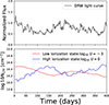 |
Fig. 7. Time-dependent photoionization simulations for the case of the DRW light curve. Top panel: DRW light curve. Bottom panel: Gas response at different ionization states, showing a positive response in the low-ionization state (log10U = −3) and a negative response in the high-ionization state (log10U = 0). In addition, in the low-ionization state the NCIV curve appears smoother, indicating that its response timescale is longer than that in the high-ionization state. |
4. Constraining the BAL gas density through the asymmetric response
In principle, an absorption line is expected to vary from one observation to the next only when the time over which the ionizing continuum varies and the time interval ΔT between the observations is longer than the t*. This asymmetry, that is, that the response timescale of high-ionization states is shorter than that of low-ionization states, suggests that in actual observations, the variations in the absorption line in high-ionization states (negative response) are expected to be more easily detected than variation in low-ionization states (positive response). This is consistent with actual observations, that is, more than 70% of the BAL in a quasar spectrum exhibit a negative response (Wang et al. 2015; He et al. 2017), based on large SDSS samples.
That the negative responses exceed 70% can impose certain limitations on the density range of BAL gas. As shown in Fig. 5, for gas with a density nH = 104 cm−3, t* for low-ionization states is about 100 days, while t* for high-ionization states is shorter than 100 days. When the observation time interval is shorter than 100 days, only responses in highly ionized states are expected to be detected, that is, only negative responses. When the gas density is nH = 106 cm−3, t* for low-ionization states is about one day, while t* for high-ionization states is shorter than one day. At this point, high- and low-ionization states can both be detected in response. We therefore evaluated the range of BAL gas density based on the fraction of negative response. In actual SDSS observations, the vast majority of observation time intervals ΔT are greater than one day. We made a rough assessment. We assumed that the fraction of BAL gas with a density below nH = 106 cm−3 was x%. If the number of intrinsic low-ionization and high-ionization states is the same, then the fraction of positive and negative responses observed for gases with a density above nH = 106 cm−3 is 0.5(1 − x%). Assuming that all gases with a density below nH = 106 cm−3 exhibit negative responses (which is an overestimate because ΔT > 1 day), then the upper limit of the observed fraction of negative responses is F. Therefore, we obtained a conservative estimate.

We therefore conclude that at least 40% of the BAL gas must have a density below nH = 106 cm−3.
Interestingly, most measured BAL outflow gas densities reported in the literature fall below 106 cm−3 (Korista et al. 2008; Moe et al. 2009; Dunn et al. 2010; Borguet et al. 2013; Lucy et al. 2014; Chamberlain et al. 2015; Arav et al. 2018; Leighly et al. 2018; Hamann et al. 2019; He et al. 2019, 2022; Xu et al. 2019; Zhao et al. 2021; Byun et al. 2022a,b, 2024). The typical gas density of an accretion disk wind (Murray et al. 1995; Proga et al. 2000) is greater than nH = 108 cm−3. At least 40% of the observed BAL gas has densities below 106 cm−3, which suggests two possibilities:
-
The accretion disk wind has propagated to larger distances, which leads to a decrease in the density.
-
Some BAL outflows may originate from larger-scale structures, such as dusty torus winds (Konigl & Kartje 1994; Scoville & Norman 1995; Elitzur & Shlosman 2006; Gallagher et al. 2015; He et al. 2022; Ishibashi et al. 2024), whose spatial scale exceeds that of the accretion disk by 100 times, which results in significantly lower densities.
For the sake of convenience in summarizing, we created a t∗(C IV) map (Fig. 8) on the plane composed of log10 U and log10 ne. The three dashed lines in the figure represent contour lines for observation time intervals ΔT = 100, 10, and 1 day, respectively. Below the respective dashed line, the observation time interval is shorter than the response timescale, that is,  , rendering it an unresponsive region. With observation time intervals of 100, 10, and 1 day, the lower-density limits that are detectable for low ionization and high ionization states are 104 cm−3, 105 cm−3, and 106 cm−3, respectively. On the one hand, given fixed observational time intervals, the lower the density of the gas, the more challenging the detection of the response of the low-ionized state. In other words, it becomes easier to detect the asymmetry of the response. On the other hand, to detect the response asymmetry of higher-density gases, a shorter observation time interval is required. This is just a simple quantitative analysis, but it indicates at least that low-density gas exists in BAL gas that is very far away from the SMBH. Some studies revealed that BAL gas likely has a low density and can exist at scales beyond the dust torus (e.g., Zhang et al. 2014; He et al. 2019, 2022; Naddaf et al. 2023; Ishibashi et al. 2024), which is consistent with our results.
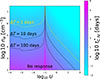 |
Fig. 8. Map of C IV response timescales on the plane of the ionization parameter and the gas density. The dashed lines represent contours that correspond to observation intervals ΔT of 1, 10, and 100 days. The dashed gold line marks one day, which is the typical minimum time interval of SDSS observations. Below each contour, the observation interval is shorter than the response timescale, indicating a nonresponsive region in which no ion concentration changes can be detected. |
5. Summary
We reported the discovery of an asymmetric response in photoionized gas. In low-ionization states, a positive correlation, called a positive response, exists between absorption lines and the ionizing source. In contrast, highly ionized states exhibit an inverse relation. Large-scale statistical analyses from the Sloan Digital Sky Survey (SDSS) revealed a striking asymmetry: More than 70% of the BAL gases in quasar host galaxies display a negative response to variations in the quasar radiation.
Our key findings are listed below.
-
Through analytical derivations and photoionization simulations of C IV, we demonstrated that the response of gas to radiation is inherently asymmetric between low- and high-ionization states. In sufficiently low-ionization conditions, that is, ni + 1/ni ≪ αi − 1/αi or Ii ≪ neαi − 1, the response timescale is given by
In contrast, for highly ionized states where ni + 1/ni ≫ αi − 1/αi or Ii ≫ neαi − 1, the response timescale becomes
Thus, in low-ionization states, the response is governed by the recombination coefficient, while in high-ionization states, it is governed by the ionization rate. This leads to shorter response timescales and a greater likelihood of observing negative responses in high-ionization states.
-
This asymmetric effect naturally explains that more than 70% of the BALs exhibit negative responses. Based on this, we further make the conservative estimate that at least 40% of the BAL gas must have a density below nH = 106 cm−3, which is consistent with the fact that most measured BAL gas densities fall below this threshold. In contrast, the typical gas density of an accretion disk wind is generally higher than nH = 108 cm−3. This discrepancy implies that either the accretion disk wind has expanded to larger scales, resulting in a lower density, or that BAL outflows may originate from more extended regions, such as dust torus winds.
While the asymmetry in the photoionization gas response offers a reasonable explanation for the observed excess of negative responses, it may not be the sole cause. To fully understand the prevalence of negative responses in absorption-line systems, further studies are needed, especially to determine whether this asymmetry persists for ions with higher-ionization potentials (e.g., O VI at 138.1 eV) or even for highly ionized iron species (> 1 keV). Another promising avenue for testing this effect is the study of absorption lines originating from stellar winds (Lamers & Cassinelli 1999) in stellar spectra.
Acknowledgments
Zhicheng He is supported by the USTC Research Launch Project KY2030000187 and the National Natural Science Foundation of China (nos. 12222304, 12192220, and 12192221).
References
- Arav, N., Edmonds, D., Borguet, B., et al. 2012, A&A, 544, A33 [NASA ADS] [CrossRef] [EDP Sciences] [Google Scholar]
- Arav, N., Liu, G., Xu, X., et al. 2018, ApJ, 857, 60 [NASA ADS] [CrossRef] [Google Scholar]
- Barkana, R., & Loeb, A. 2001, Phys. Rep., 349, 125 [NASA ADS] [CrossRef] [Google Scholar]
- Borguet, B. C., Arav, N., Edmonds, D., Chamberlain, C., & Benn, C. 2013, ApJ, 762, 49 [NASA ADS] [CrossRef] [Google Scholar]
- Byun, D., Arav, N., & Hall, P. B. 2022a, MNRAS, 517, 1048 [NASA ADS] [CrossRef] [Google Scholar]
- Byun, D., Arav, N., & Walker, A. 2022b, MNRAS, 516, 100 [NASA ADS] [CrossRef] [Google Scholar]
- Byun, D., Arav, N., Sharma, M., Dehghanian, M., & Walker, G. 2024, A&A, 684, A158 [NASA ADS] [CrossRef] [EDP Sciences] [Google Scholar]
- Chamberlain, C., Arav, N., & Benn, C. 2015, MNRAS, 450, 1085 [NASA ADS] [CrossRef] [Google Scholar]
- Dunn, J. P., Bautista, M., Arav, N., et al. 2010, ApJ, 709, 611 [NASA ADS] [CrossRef] [Google Scholar]
- Elitzur, M., & Shlosman, I. 2006, ApJ, 648, L101 [Google Scholar]
- Fabian, A. C. 2012, ARA&A, 50, 455 [Google Scholar]
- Fan, X., Carilli, C., & Keating, B. 2006, ARA&A, 44, 415 [NASA ADS] [CrossRef] [Google Scholar]
- Fan, X., Bañados, E., & Simcoe, R. A. 2023, ARA&A, 61, 373 [NASA ADS] [CrossRef] [Google Scholar]
- Ferland, G., Chatzikos, M., Guzmán, F., et al. 2017, Rev. Mex. Astron. Astrofis., 53, 385 [Google Scholar]
- Gallagher, S., Everett, J., Abado, M., & Keating, S. 2015, MNRAS, 451, 2991 [NASA ADS] [CrossRef] [Google Scholar]
- García, J., Dauser, T., Reynolds, C., et al. 2013, ApJ, 768, 146 [NASA ADS] [CrossRef] [Google Scholar]
- Hamann, F., Herbst, H., Paris, I., & Capellupo, D. 2019, MNRAS, 483, 1808 [NASA ADS] [CrossRef] [Google Scholar]
- He, Z.-C., Bian, W.-H., Jiang, X.-L., & Wang, Y.-F. 2014, MNRAS, 443, 2532 [Google Scholar]
- He, Z.-C., Bian, W.-H., Ge, X., & Jiang, X.-L. 2015, MNRAS, 454, 3962 [Google Scholar]
- He, Z., Wang, T., Zhou, H., et al. 2017, ApJS, 229, 22 [NASA ADS] [CrossRef] [Google Scholar]
- He, Z., Wang, T., Liu, G., et al. 2019, Nat. Astron., 3, 265 [NASA ADS] [CrossRef] [Google Scholar]
- He, Z., Liu, G., Wang, T., et al. 2022, Sci. Adv., 8, eabk3291 [NASA ADS] [CrossRef] [Google Scholar]
- He, Z., Wang, T., & Ferland, G. J. 2025, ApJ, 986, 164 [Google Scholar]
- Hemler, Z., Grier, C., Brandt, W., et al. 2019, ApJ, 872, 21 [NASA ADS] [CrossRef] [Google Scholar]
- Ishibashi, W., Fabian, A., & Hewett, P. 2024, MNRAS, 533, 4384 [NASA ADS] [CrossRef] [Google Scholar]
- Jakobsen, P., Boksenberg, A., Deharveng, J., et al. 1994, Nature, 370, 35 [NASA ADS] [CrossRef] [Google Scholar]
- Kaastra, J., Detmers, R., Mehdipour, M., et al. 2012, A&A, 539, A117 [NASA ADS] [CrossRef] [EDP Sciences] [Google Scholar]
- Kelly, B. C., Bechtold, J., & Siemiginowska, A. 2009, ApJ, 698, 895 [Google Scholar]
- Konigl, A., & Kartje, J. F. 1994, ApJ, 434, 446 [NASA ADS] [CrossRef] [Google Scholar]
- Korista, K. T., Bautista, M. A., Arav, N., et al. 2008, ApJ, 688, 108 [NASA ADS] [CrossRef] [Google Scholar]
- Kormendy, J., & Ho, L. C. 2013, ARA&A, 51, 511 [Google Scholar]
- Kozłowski, S., Kochanek, C. S., Udalski, A., et al. 2009, ApJ, 708, 927 [Google Scholar]
- Kriss, G., Shull, J., Oegerle, W., et al. 2001, Science, 293, 1112 [Google Scholar]
- Krolik, J. H., & Kriss, G. A. 1995, ApJ, 447, 512 [NASA ADS] [CrossRef] [Google Scholar]
- Krongold, Y., Nicastro, F., Elvis, M., et al. 2007, ApJ, 659, 1022 [NASA ADS] [CrossRef] [Google Scholar]
- Lamers, H. J., & Cassinelli, J. P. 1999, Introduction to Stellar Winds (Cambridge University Press) [Google Scholar]
- Leighly, K. M., Terndrup, D. M., Gallagher, S. C., Richards, G. T., & Dietrich, M. 2018, ApJ, 866, 7 [NASA ADS] [CrossRef] [Google Scholar]
- Loeb, A., & Barkana, R. 2001, ARA&A, 39, 19 [NASA ADS] [CrossRef] [Google Scholar]
- Lu, W.-J., Lin, Y.-R., & Qin, Y.-P. 2018, MNRAS, 473, L106 [Google Scholar]
- Lucy, A. B., Leighly, K. M., Terndrup, D. M., Dietrich, M., & Gallagher, S. C. 2014, ApJ, 783, 58 [NASA ADS] [CrossRef] [Google Scholar]
- MacLeod, C. L., Ivezić, Ž., Kochanek, C., et al. 2010, ApJ, 721, 1014 [Google Scholar]
- Moe, M., Arav, N., Bautista, M. A., & Korista, K. T. 2009, ApJ, 706, 525 [NASA ADS] [CrossRef] [Google Scholar]
- Murray, N., Chiang, J., Grossman, S., & Voit, G. 1995, ApJ, 451, 498 [NASA ADS] [CrossRef] [Google Scholar]
- Naddaf, M. H., Martinez-Aldama, M. L., Marziani, P., et al. 2023, A&A, 675, A43 [NASA ADS] [CrossRef] [EDP Sciences] [Google Scholar]
- Netzer, H. 2013, The Physics and Evolution of Active Galactic Nuclei (Cambridge University Press) [Google Scholar]
- Nicastro, F., Fiore, F., Perola, G. C., & Elvis, M. 1999, ApJ, 512, 184 [NASA ADS] [CrossRef] [Google Scholar]
- Osterbrock, D. E., & Ferland, G. J. 2006, Astrophysics of Gaseous Nebulae and Active Galactic Nuclei, 2nd edn. (University Science Books) [Google Scholar]
- Proga, D., Stone, J. M., & Kallman, T. R. 2000, ApJ, 543, 686 [Google Scholar]
- Rogantini, D., Mehdipour, M., Kaastra, J., et al. 2022, ApJ, 940, 122 [NASA ADS] [CrossRef] [Google Scholar]
- Sadaula, D. R., & Kallman, T. R. 2024, ApJ, 960, 120 [Google Scholar]
- Sadaula, D. R., Bautista, M. A., Garcia, J. A., & Kallman, T. R. 2023, ApJ, 946, 93 [NASA ADS] [CrossRef] [Google Scholar]
- Scoville, N., & Norman, C. 1995, ApJ, 451, 510 [Google Scholar]
- Tilvi, V., Malhotra, S., Rhoads, J., et al. 2020, ApJ, 891, L10 [NASA ADS] [CrossRef] [Google Scholar]
- Veilleux, S., Maiolino, R., Bolatto, A. D., & Aalto, S. 2020, Astron. Astrophys. Rev., 28, 1 [Google Scholar]
- Verner, D., Ferland, G., Korista, K., & Yakovlev, D. 1996, ApJ, 465, 487 [Google Scholar]
- Vivek, M. 2019, MNRAS, 486, 2379 [Google Scholar]
- Wang, T., Yang, C., Wang, H., & Ferland, G. 2015, ApJ, 814, 150 [Google Scholar]
- Wang, F., Yang, J., Fan, X., et al. 2021, ApJ, 907, L1 [Google Scholar]
- Xu, X., Arav, N., Miller, T., & Benn, C. 2019, ApJ, 876, 105 [NASA ADS] [CrossRef] [Google Scholar]
- Yung, L. A., Somerville, R. S., Finkelstein, S. L., et al. 2020, MNRAS, 496, 4574 [NASA ADS] [CrossRef] [Google Scholar]
- Zhang, S., Wang, H., Wang, T., et al. 2014, ApJ, 786, 42 [NASA ADS] [CrossRef] [Google Scholar]
- Zhao, Q., He, Z., Liu, G., et al. 2021, ApJ, 906, L8 [Google Scholar]
- Zheng, W., Kriss, G., Deharveng, J.-M., et al. 2004, ApJ, 605, 631 [Google Scholar]
All Figures
|
Fig. 1. Schematic diagram of the variation in the ion column density with ionization luminosity. The column density of a specific ion in the plasma initially increases to a peak and then decreases with the rise in ionization level. The vertical dashed line represents the peak position. |
| In the text | |
|
Fig. 2. Schematic diagram of the asymmetric effect of ion response timescale. The vertical dashed line is the boundary between the low ionized state and the high ionized state. In a sufficiently low ionization state, i.e., ni + 1/ni ≪ αi − 1/αi or Ii ≪ neαi − 1, the response timescale is ti* = 1/(fneαi − 1). In a sufficiently high ionization state, in contrast, i.e., ni + 1/ni ≫ αi − 1/αi or Ii ≫ neαi − 1, the response timescale is |
| In the text | |
|
Fig. 3. Nonmonotonic dependence of the carbon ion column densities on the ionization parameter. The column densities of carbon ions first increase and then decrease with the ionization parameter. |
| In the text | |
|
Fig. 4. Recombination coefficients and ion concentrations predicted by equilibrium-state photoionization simulations. The recombination coefficients of C III and C IV, as well as the population density ratio nC V/nC IV under different ionization parameters, were obtained from equilibrium photoionization simulations using Cloudy version c17 (Ferland et al. 2017). |
| In the text | |
|
Fig. 5. Response timescale of C IV under different ionization parameters. The black and red curves correspond to gas densities of 104 cm−3 and 106 cm−3, respectively. The timescale exhibits strong asymmetry: the response timescale of highly ionized states is significantly shorter than that of low-ionized states. If the observational time interval falls within 1–1000 days, this asymmetry would not be detectable for gas at a density of 106 cm−3, but it would be observable for gas with a density of 104 cm−3. |
| In the text | |
|
Fig. 6. Time-dependent photoionization simulations for the case of the light curve of the step function. At t = 0, the radiation flux is suddenly increased from 1 to 2, corresponding to a change amplitude of f = 1. This leads to a positive response in the low-ionization state (log10U = −3) and a negative response in the high-ionization state (log10U = 0). The dashed red lines represent the response timescales at the initial time predicted by Equation (11). The response timescales for log10U = −3 and log10U = 0 are 48.3 days and 5.5 days, respectively, indicating that the C IV concentration evolves more rapidly at higher ionization (log10U = 0). |
| In the text | |
|
Fig. 7. Time-dependent photoionization simulations for the case of the DRW light curve. Top panel: DRW light curve. Bottom panel: Gas response at different ionization states, showing a positive response in the low-ionization state (log10U = −3) and a negative response in the high-ionization state (log10U = 0). In addition, in the low-ionization state the NCIV curve appears smoother, indicating that its response timescale is longer than that in the high-ionization state. |
| In the text | |
|
Fig. 8. Map of C IV response timescales on the plane of the ionization parameter and the gas density. The dashed lines represent contours that correspond to observation intervals ΔT of 1, 10, and 100 days. The dashed gold line marks one day, which is the typical minimum time interval of SDSS observations. Below each contour, the observation interval is shorter than the response timescale, indicating a nonresponsive region in which no ion concentration changes can be detected. |
| In the text | |
Current usage metrics show cumulative count of Article Views (full-text article views including HTML views, PDF and ePub downloads, according to the available data) and Abstracts Views on Vision4Press platform.
Data correspond to usage on the plateform after 2015. The current usage metrics is available 48-96 hours after online publication and is updated daily on week days.
Initial download of the metrics may take a while.