| Issue |
A&A
Volume 703, November 2025
|
|
|---|---|---|
| Article Number | A219 | |
| Number of page(s) | 9 | |
| Section | Planets, planetary systems, and small bodies | |
| DOI | https://doi.org/10.1051/0004-6361/202556250 | |
| Published online | 18 November 2025 | |
HDO and SO2 thermal mapping on Venus
VII. SO2 variations with altitude and influence of the solar cycle
1
LESIA, Observatoire de Paris, PSL University, CNRS, Sorbonne Université, Université de Paris,
92195
Meudon,
France
2
SwRI, Div. 15,
San Antonio,
TX
78228,
USA
3
LATMOS/IPSL, UVSQ Université Paris-Saclay, Sorbonne Université, CNRS,
78280
Guyancourt,
France
4
Department of Astrophysics and Atmospheric Science, Kyoto Sangyo University,
603-8555
Kyoto,
Japan
5
Department of Space Research and Technology, Technical University of Denmark,
Denmark
★ Corresponding author.
Received:
4
July
2025
Accepted:
17
October
2025
Abstract
Context. Sulfur dioxide and water are two key minor species of Venus’ atmosphere which drive its chemical evolution. However, the long-term variations in the SO2 abundance at the cloud top, measured since 1978, remain unexplained.
Aims. In order to address this question, since 2012, we have performed a ground-based campaign to monitor the SO2 and H2O abundances in the region of the Venus upper cloud, using the TEXES (Texas Echelon Cross-Echelle Spectrograph) imaging spectrometer at the NASA InfraRed Telescope Facility (IRTF, Mauna Kea Observatory).
Methods. Observations were recorded in three spectral ranges: (1) the 1342–1348 cm−1 (7.4 µm) spectral range, where SO2, CO2 and HDO (used as a proxy for H2O) transitions are observed at an altitude of about 62 km, defined in our model as the cloud top; (2) the 529–530 cm−1 range (18.9 µm), where SO2 and CO2 are probed within the clouds a few kilometers below the cloud top; (3) the 1160–1165 cm−1 range (8.6 µm) where the weak SO2 v1 band is used to probe a few kilometers above the cloud top.
Results. We present here the data recorded from July 2023 to February 2025. As was reported in our previous analyses, the SO2 maps show evidence for the formation of SO2 plumes, mostly located around the equator, with a typical lifetime of a few hours; large variations in the SO2 disk-integrated abundance also appear on a timescale of a few months. In contrast, the H2O abundance is remarkably uniform over the disk and shows moderate variations as a function of time. The present dataset shows for the first time the detection of the SO2 v1 band above the cloud top. The simultaneous analysis of the three SO2 bands allows us to constrain the SO2 volume mixing ratio within and above the cloud. In addition, we have re-analyzed the long-term evolution of the SO2 and H2O mixing ratios at the cloud top. Between 2012 and 2023, the SO2 abundance is clearly anti-correlated with the solar activity, which suggests that photochemistry, activated by the solar UV flux, is the main mechanism driving the SO2 abundance. After 2023, SO2 exhibits strong variations with a timescale as short as two months, which suggest that other mechanisms are involved. Finally, we have re-analyzed the distribution of SO2 at the cloud top as a function of the local time, using three different data subsets (2012–2017, 2021–2022, 2023–2025). In spite of the differences, there is a general trend toward a minimum value around 12:00 and maxima around 5:00 and 17:00.
Conclusions. Our data suggest that the solar cycle plays an important role in the long-term evolution of SO2 and H2O at the cloud top. In addition, in some cases, other mechanisms are probably also involved, possibly associated with dynamical motions, implying sublimation/condensation processes and/or gas-aerosol conversion.
Key words: planets and satellites: atmospheres / planets and satellites: composition / planets and satellites: terrestrial planets / planets and satellites: individual: Venus
© The Authors 2025
 Open Access article, published by EDP Sciences, under the terms of the Creative Commons Attribution License (https://creativecommons.org/licenses/by/4.0), which permits unrestricted use, distribution, and reproduction in any medium, provided the original work is properly cited.
This article is published in open access under the Subscribe to Open model. This email address is being protected from spambots. You need JavaScript enabled to view it. to support open access publication.
1 Introduction
Water and sulfur dioxide are the drivers of Venus’ atmospheric chemistry (Krasnopolsky 1986, Krasnopolsky 2007, 2010; Mills et al. 2007; Zhang et al. 2012). Below the clouds, both species are present with relatively large abundances (about 30 ppmv and 130 ppmv, respectively, Bézard and De Bergh 2012; Marcq et al. 2018) and, at low latitude, are transported upward by Hadley convection. Following the SO2 photodissociation and the combination of SO3 with H2O, sulfuric acid H2SO4 is formed and condenses in the form of binary (H2SO4−H2O) aerosols in the cloud deck (Stolzenbach et al. 2023). Above the cloud top, the volume mixing ratios of H2O and SO2 drop drastically to about 1–3 ppmv (Fedorova et al. 2008; Belyaev et al. 2012) and 10–1000 ppbv (Zasova et al. 1993; Marcq et al. 2013, 2020; Vandaele et al. 2017a,b), respectively. Since the condensation mechanism consumes 2 H2O molecules for one SO2 molecule, another unknown mechanism is required to trap the extra SO2 within the clouds.
Both species have been extensively monitored over several decades, with Pioneer Venus, the Venera 15 spacecraft, Venus Express and Akatsuki using imaging and spectroscopy in the ultraviolet and infrared ranges. As a complement to these datasets, since 2012, we have been using the TEXES (Texas Echelon Cross-Echelle Spectrograph) imaging spectrometer at the NASA InfraRed Telescope Facility (IRTF, Mauna Kea Observatory) to map SO2 and H2O at the cloud top of Venus (using HDO as a proxy of H2O) and to monitor the behavior of these two species as a function of time. Eighteen runs have been recorded between January 2012 and July 2022 (Encrenaz et al. 2023, hereafter referred as E23, and references therein). The main result of these studies is that SO2 and H2O exhibit very different behaviors. H2O is always uniformly distributed over the disk and shows moderate variations on the long term; in contrast, the SO2 maps most often show sporadic plumes which appear and disappear with a typical timescale of a few hours; these features are probably the signature of dynamical activity within the clouds. The disk-integrated SO2 abundance also shows strong variations over the long term, with a contrast factor of about 10 between the minimum value observed in February 2014 and the maximum value of July 2018 (also reobserved early 2025). A plausible explanation for the absence of H2O plumes is the fact that the H2O mixing ratio is globally constant within and above the clouds, so it is not a good tracer of vertical motions.
In this paper, we present the results obtained during the seven new observing runs recorded between March 2023 and March 2025. The observations are described in Section 2, showing in particular the detection of the SO2 ν1 band at 8.6 µm. These data are used to constrain the SO2 vertical profile at the three altitudes probed by the three SO2 bands (Section 3). Then, we use the whole TEXES data set (2012–2022) at 7.4 µm to study the long-term evolution of H2O and SO2 (Section 4). Finally, we update our statistical analysis of the SO2 plumes, regarding their appearance as a function of the local time (Section 5). Results and conclusions are presented in Section 6.
2 The data
TEXES (Texas Echelon Cross Echelle Spectrograph) is an imaging high-resolution thermal infrared spectrometer in operation at the NASA InfraRed telescope Facility (Lacy et al. 2002), which combines high spectral (R = 80 000 at 7 µm) and spatial (around 1 arcsec) capabilities. As for our previous observations, we selected three spectral ranges: (1) 1342–1348 cm−1 (7.4 µm), (2) 529–530 cm−1 (18.9 µm) and (3) 1160–1165 cm−1 (8.6 µm). The first setting (7.4 µm) has been used since 2012 to monitor the mixing ratios of SO2 and HDO at the altitude level z = 62 km, referred in our model as the cloud top. The second setting (18.9 µm) has been also regularly used to monitor the SO2 abundance a few kilometers below the cloud top (z = 57 km). The third setting (8.6 µm) probes a few kilometers above the cloud top (z = 67 km) and also contains the weak ν1 band of SO2. This band is difficult to detect on Venus, both because of its intrinsic weakness and because the sharp depletion of SO2 above the cloud top (E23). However, when the SO2 abundance at the cloud top is over a few hundred ppbv, as in 2018 and 2019, the band might be detectable or its absence might bring a constraint on the SO2 vertical gradient above the clouds. For this reason, we have observed this spectral range regularly since June 2021.
Seven runs have taken place in March, July, October, and December 2023, in February 2024, and in January and March 2025; the observing parameters are listed in Table 1. The length and the width of the slit were respectively 6.0 and 1.0 arcsec at 7.4 µm, 12.0 and 2.0 arcsec at 18.9 µm, and 8.0 and 1.0 arcsec at 8.6 µm. As we did previously, we aligned the slit along the North-South celestial axis and we shifted it from west to east, with a step of half the slit width and an integration time of 2 seconds per position, to cover the planet in longitude from limb to limb, and to add a few pixels on the sky beyond each limb for sky subtraction. Since the rotation axis of Venus is close to the celestial axis, each scan corresponds to a given latitude range of about 6 arcsec. As the diameter of Venus was always larger than the slit length, we multiplied the scans to cover the full latitude range from North to South with some overlap. The TEXES data cubes were calibrated using the standard radiometric method (Lacy et al. 2002; Rohlfs and Wilson 2004). Calibration frames consisting of three measurements (black chopper blade, sky and low-emissivity chopper blade) are systematically taken before each observing scan, and the difference (black-sky) is taken as a flat field. As the atmospheric correction, however, is not complete for all terrestrial atmospheric lines (partly because these lines are not all formed at the same atmospheric levels, and thus have different temperatures), the HDO, SO2 and CO2 lines selected for our study are located outside the atmospheric features.
Figure 1 shows representative disk-integrated spectra corresponding to the 2023–2025 runs in the 7.4 and 18.9 µm ranges. The 7.4-µm spectral range (1344.8–1345.4 cm−1) includes several weak SO2 transitions, two weak CO2 lines and one weak HDO line. As in our previous studies (see E23 and references therein), we used the HDO line at 1344.90 cm−1, the SO2 multiplet at 1345.1 cm−1 and the CO2 line at 1345.22 cm−1. In the 18.9 µm range (529–530 cm−1) weak transitions of SO2 and CO2 are found. We used the SO2 multiplet at 529.69 cm−1 and the CO2 line at 529.81 cm−1. It immediately appears, in both datasets, that the SO2 lines depths show strong variations from run to run: they are as strong as the neighbor CO2 line at maximum, and almost disappear at minimum. In order to estimate the H2O and SO2 mixing ratios, as was discussed in earlier papers (see e.g., E23), we use the ratios of the SO2/CO2 and HDO/CO2 line depths which provide a good approximation of the SO2 and H2O mixing ratios at the altitude probed in each spectral range. The HDO/H2O ratio at the cloud deck and above is estimated to 200 times the terrestrial value VSMOW (Fedorova et al. 2008; E23).
In addition to the 7.4 and 18.9 µm spectral ranges, since 2021, we have observed the 1160–1165 cm−1 range, at 8.6 µm, which contains some transitions of the SO2 ν1 band at 8.6 µm (Zasova et al. 1993). As mentioned above, its detection is difficult. We failed to detect it in 2021 and 2022, which was not surprising as the SO2 abundance at that time was especially low. As shown in Figure 1, the SO2 abundance has been very high in July 2023, October 2023 and January 2025. As a consequence, the ν1 band has been actually detected in each of these three observing runs. This is its first ground-based detection; the only earlier report was in 1983 by the Venera 15 far infrared interferometer, in some specific locations on the planet (Zasova et al. 1993).
Figure 2 shows three disk-integrated spectra of Venus recorded in the 1160–1163 cm−1 spectral range, in July 2023, October 2023 and January 2025, respectively. The spectrum is fully dominated by terrestrial atmospheric lines, mostly due to nitrous oxide and ozone. As expected, the SO2 lines are very weak, and were not detected in March 2023, December 2023 and February 2024. We choose to study the spectral region around the SO2 transition at 1160.7733 cm−1 (I = 5.57×10⁻²¹ cm/mol, E = 74.66 cm−1) which is well separated from terrestrial lines whatever the Doppler shift is (Fig. 2).
Summary of TEXES runs in 2023–2025.
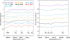 |
Fig. 1 Examples of disk-integrated spectra of Venus (normalized radiance) recorded in 2023–2025. Left: 1344.85–1345.30 cm−1 spectral range (7.4 µm). The spectra are shifted by −0.2 in vertical scale for clarity. Right: examples of disk-integrated spectra of Venus (normalized radiance) between 529.65 and 529.85 cm−1 (18.9 µm). The spectra are shifted by −0.1 in vertical scale for clarity. |
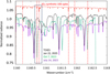 |
Fig. 2 Disk-integrated spectra of Venus between 1160 and 1163 cm−1 (8.6 µm) recorded on July 14, 2023, October 7, 2023 and January 22, 2025. The positions of the strongest SO2 lines are indicated in red by vertical dashed lines. The terrestrial lines coincide in the July 2023 and January 2025 because the Doppler shift is the same for both datasets, while it is different for the spectrum taken in October 2023. The spectra are dominated by terrestrial atmospheric absorption features, mostly N2O and O3. The black rectangle shows the spectral range used for our analysis. |
3 The SO2 vertical distribution
As was discussed in our earlier publications (see e.g., E23), observing Venus at three different infrared wavelengths allows us to probe different atmospheric levels, because of the variations in the H2SO4 extinction coefficient that is maximum around 8.6 µm and minimum around 19 µm, while its value at 7.4 µm is intermediate. Based on a thermal profile inferred from CO2 TEXES observations (Giles et al. 2022), our previous analyses of the CO2 lines at 7.4 and 18.9 µm have shown that the penetration levels at these two wavelengths are located near P = 250 mbar (T = 241 K, z = 57 km) at 18.9 µm and P = 100 mbar (T = 230 K, z = 62 km, referred as the cloud top in our model) at 7.4 µm. Note that this definition of the cloud top is somehow arbitrary: it is the penetration level (τ = 1) at 7.4 µm and is slightly model dependent, as the CO2 line profiles give access to the pressure, and not the altitude; in addition, this level shows slight variations from run to run. We note that our reference level is a few km lower than the cloud top defined at this wavelength by Titov et al. (2018) for the standard model, and better fits the model with enriched upper haze.
In our earlier work, we have inferred the SO2 mixing ratio at z = 57 and 62 km from the analysis of the SO2 lines. The detection of the SO2 lines at 8.6 µm gives us a new constrain on the SO2 vertical distribution above the cloud top. From the shape of the SO2 lines (broader than the CO2 lines) at 7.4 and 18.9 µm, it could be seen that depletion of SO2 had to occur a few kilometers above the cloud top. In the model described in E23, we introduced this cutoff at z = 70 km (T = 204 K, P = 23 mbar). Such a strong depletion with altitude is also observed in the UV range (Marcq et al. 2020). Using our radiative transfer calculations, we derived the HDO and SO2 mixing ratios from the line depth ratios of weak HDO and SO2 lines divided by a weak nearby CO2 line, as we did in our earlier studies (E23 and references therein). This simple method has the advantage of providing a good estimate of the H2O and SO2 mixing ratios, independently of the atmospheric parameters and the airmass factor. We have been using it to study the long-term evolution of the two species at the cloud top, and to obtain maps of the HDO and SO2 mixing ratios at 7.3 and 18.9 µm. For the conversion from the line depth ratios (ldr) into the volume mixing ratios (vmr), the following equations are used (E23):
At 7.4 µm (1345 cm−1):
vmr(SO2)(ppbv) = ldr(SO2) × 600.0
vmr(H2O)(ppmv) = ldr (HDO) × 1.5.
At 19 µm(530 cm−1):
vmr(SO2)(ppbv) = ldr(SO2) × 500.0.
In the case of the 8.6-µm spectra, we cannot apply this method, unfortunately, because there is no CO2 transition available in this spectral range. The only information about the penetration level at 8.6 µm comes from the infrared spectrum of the H2SO4 absorption coefficient (Zasova et al. 1993) which indicates that it is higher at 8.6 µm than at 7.4 µm. Then, we deduce that the penetration level at 8.6 µm must be a few km higher than the one at 7.4 µm. We modeled the SO2 line around 1160.77 cm−1 assuming different altitude levels and different values of the SO2 vmr above the cloud top and trying to fit the three disk-integrated spectra simultaneously. Our radiative transfer code is described in earlier publications (E23 and references therein). It is a forward model and no retrieval algorithm is used in our study. Our model consists in a line-by-line calculation without scattering. Spectroscopic data are taken from the GEISA data base (Jacquinet-Husson et al. 2018). In the case of SO2, for which the broadening coefficients by CO2 are not given in the database, as in our earlier studies, we multiplied the broadening coefficients by N2 by a factor 1.4 (Nakazawa and Tanaka 1982).
On the basis of the equations mentioned above, the SO2 vmr was set to 500 ppbv at 57 km and 400 ppbv at 62 km for the three data sets showing the SO2 line at 8.6 µm. An example of fit is shown in Figures 3–5. In this model, a cutoff is applied at z = 72 km (T = 201 K, P = 13 mbar). The influence of this parameter on the results is discussed in Section 5. From the direct comparison between the data and the models, in Figures 3–5, it can be seen that, at 7.4 and 18.9 µm, the best fit is obtained with a SO2 vmr of 150 ppbv, while the 8.6 µm spectrum favors a SO2 vmr of 100 ppbv. This discrepancy probably means that the choice of the SO2 cutoff altitude (fixed, in our earlier studies, from the shapes of the SO2 lines at 7.4 and 18.9 µm) is not optimized. It also probably illustrates that our model is too simple and does not account, in particular, for possible inhomogeneities over the Venus disk. From Figures 3–5, we conclude that a SO2 vmr between 100 and 150 ppbv at an altitude of 67 km (T = 223 K, P = 40 mbar), associated with a SO2 cutoff at z = 72 km, provides a reasonable fit of the three spectra. It must be reminded that this solution is not unique, as the SO2 measurement at 8.7 µm only provides a constraint upon the SO2 column density. The SO2 vmr estimated at 8.7 µm thus depends on both the altitude of the penetration level (here 67 km) and the altitude of the SO2 cutoff (here z = 72 km).
As the 8.6 µm spectral range does not include CO2 transitions, we cannot obtain SO2 maps at 67 km, as we did at 57 and 62 km using the 18.9 µm and 7.4 µm data. We cannot either determine precisely the penetration level at 8.6 µm. Still, we can use the depth of the SO2 transition at 1160.77 cm−1 as an indicator of the SO2 abundance a few kilometers above our reference level probed at 7.4 µm (in our model, z = 62 km). Figures 6–8 show these maps, compared to the maps of the SO2 volume mixing ratio obtained at 7.4 and 19 µm, from the data shown in Figure 1, using the transitions mentioned above. It can be seen that, not surprisingly, the SO2 spatial distribution at 62 km is usually well correlated with those observed at deeper levels. However, a remarkable behavior is observed in October 2023 (Fig. 7). As was discussed in earlier papers, the distribution of the SO2 plumes is usually concentrated around the equator (E23). In October 2023, the SO2 plumes are structured in two parallel bands located at mid-latitude, over a longitude range of about 120 degrees. This band structure appears on October 3 and is observed over 4 consecutive days; indeed, as shown by the different 18.9 µm SO2 maps between October 3 and October 7, it rotates by 90 degrees per day, following the 4-day rotation of the clouds. The structure also appears, although less clearly, on the SO2 maps at higher altitudes; on October 7, the SO2 map at z = 67 km shows clearly the band structure with a strong enhancement in the northern hemisphere. The longevity of this dynamical structure is actually exceptional, as the life time of SO2 plumes are usually shorter than a day (E23). It can be noticed also that the parallel latitudinal structure is not observed on the continuum maps which reflect the temperature field at the three altitudes probed in this study.
In order to investigate in more detail the anomaly observed in October 2023, we have selected, on the October 7 map, two locations close to the central meridian, at the disk center and at mid-northern latitude (Fig. 7). Figures 9–11 show the spectra of these two regions in the three spectral ranges. As expected from Figure 7, very strong variations are observed in the SO2 absorptions between the center and the northern hemisphere. In particular, the very low SO2 abundance observed at 18.9 µm (z = 57 km) at the disk center seems difficult to reconcile with the two other spectra; this discrepancy is discussed in Section 6.
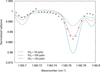 |
Fig. 3 Disk-integrated spectrum of Venus between 1160.69 and 1160.80 cm−1 (8.6 µm) recorded on July 14. Models: SO2(57 km) = 500 ppbv, SO2(62 km) = 400 ppbv, SO2(67 km) = 50 ppbv (green), 100 ppbv (red) and 150 ppbv (blue). |
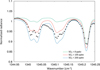 |
Fig. 4 Disk-integrated spectrum of Venus between 1344.95 and 1345.25 cm−1 (7.4 µm) recorded on July 14, 2023. Models: SO2(57 km) = 500 ppbv, SO2(62 km) = 400 ppbv, SO2(67 km) = 0 ppbv (green), 100 ppbv (red) and 200 ppbv (blue). |
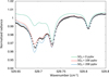 |
Fig. 5 Disk-integrated spectrum of Venus between 529.65 and 529.85 cm−1 (18.9 µm) recorded on July 14, 2023. Models: SO2(57 km) = 500 ppbv, SO2(62 km) = 400 ppbv, SO2 (67 km) = 0 ppbv (green), 100 ppbv (red) and 200 ppbv (blue). |
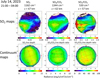 |
Fig. 6 Top: SO2 maps recorded on July 14, 2023. Left: z = 67 km (SO2 line depth); middle: z = 62 km (SO2/CO2 line depth ratio); right: z = 57 km (SO2/CO2 line depth ratio). Disk-integrated spectra corresponding to these maps are shown in Figs. 3–5. Bottom: continuum maps recorded on July 14, 2023 at z = 67 km (left), 62 km (middle) and 57 km (right). |
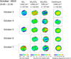 |
Fig. 7 SO2 maps recorded on October 3–7, 2023. Left: z = 67 km (SO2 line depth); middle: z = 62 km (SO2/CO2 line depth ratio); next: z = 57 km (SO2/CO2 line depth ratio). Last right column: continuum maps recorded on October 3–7, 2023 at z = 62 km. The black crosses on the October 7 SO2 maps indicate the positions corresponding to the spectra shown in Figs. 9–11 (disk center and 30°N latitude). |
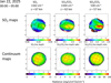 |
Fig. 8 Top: SO2 maps recorded on January 22, 2025. Left: z = 67 km (SO2 line depth); middle: z = 62 km (SO2/CO2 line depth ratio); right: z = 57 km (SO2/CO2 line depth ratio). Bottom: continuum maps recorded on January 22, 2025 at z = 67 km (left), 62 km (middle) and 57 km (right). |
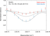 |
Fig. 9 Spectra of Venus between 1160.75 and 1160.79 cm−1 (8.6 µm) recorded on October 7, 2023 at the disk center (red points) and at 30N latitude (blue points). Models: SO2(57 km) = 500 ppbv, SO2(62 km) = 400 ppbv. From top to bottom: SO2(67 km) = 50, 100 and 200 ppbv. |
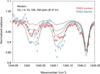 |
Fig. 10 Spectra of Venus between 1344.95 and 1345.25 cm−1 (7.4 µm) recorded on October 7, 2023 at the disk center (red points) and at 30°N latitude (blue points). Models: SO2(57 km) = 500 ppbv, SO2(62 km) = 400 ppbv. From top to bottom: SO2(67 km) = 0, 50, 100 and 200 ppbv. |
4 Long-term variations in SO2 and H2O
Figure 12 shows the temporal variations in the disk-integrated H2O and SO2 mixing ratios at the cloud top (z = 62 km) derived from the 7.4-µm data. The evolution of the solar activity is shown for comparison.
In our previous analysis (E23), we reported a clear anti-correlation of the two molecules (correlation coefficient = −0.9) between 2014 and 2019. Since this period, H2O and SO2 have evolved differently, with strong temporal variations in the SO2 abundance (by a factor as much as 5), over timescales as short as two months, while the H2O abundance has remained more or less constant. It is interesting to note that, between 2012 and 2023, the SO2 abundance is anti-correlated with the solar activity, while the H2O abundance shows a correlation with the solar cycle between 2012 and 2023. This strongly suggests that, in this period, photochemistry is the main mechanism driving the behaviors of SO2 and H2O at the cloud top of Venus. Indeed, an increase in the solar UV flux is expected to enhance the photodissociation of SO2, decreasing its abundance. As shown by Parkinson et al. (2015), H2O and SO2 are expected to regulate themselves through the formation of H2SO4 and this effect could be responsible for the anti-correlation observed between the two molecules.
We then wondered if the effect of the solar cycle could have been visible in the past. There is no long-term record of the water abundance at the cloud top (as no strong variations have been observed), but the SO2 abundance has been measured since 1978, thanks to the UV measurements of Pioneer Venus, and later Venus Express and Akatsuki. Figure 13 shows the long-term evolution of SO2 from 1978 to now, compared to the solar cycle. Because the UV data probe an altitude slightly higher than the TEXES data (around z = 70 km), we normalized our data by adjusting them to the Venus Express data taken in 2012–2015 by dividing them by a factor 3, which is consistent with the SO2 vmr inferred from our data at 8.6 µm, as was discussed above. It can be seen that the strong decrease of the SO2 abundance observed by Pioneer Venus in 1978–1982 can be explained by the strong increase in the solar UV flux during these periods.
However, the anti-correlation between the SO2 abundance and the solar activity is not observed at all times, in particular, the strong SO2 decrease observed by Venus Express in 2006–2009 corresponds to a minimum of the solar activity; in addition, no increase in SO2 is observed in 1985–1987 when the solar activity is at its minimum. This suggests that the solar cycle is not the only driver of the SO2 long-term evolution. This conclusion is also supported by the TEXES data after 2023, suggesting that a change of regime has occurred at that time. The strong fluctuations of the SO2 abundances, on timescales of only two months, cannot be explained by the solar cycle. In order to study which parameter could be responsible for these fluctuations, we have plotted the SO2 abundance at the cloud top as a function of the Venus diameter, the local time at the disk center and the longitude at the disk center (Fig. 14). There is no obvious relationship between any of these parameters with the SO2 abundance. It can be observed that, after 2023, the high values of SO2 are found when the nightside of Venus is observed (maximum diameter); however, the opposite is observed in January 2021, so no firm conclusion can be drawn.
Finally, we have used the long-term variations in the SO2 vmr at z = 57 km, measured at 18.9 µm, to study the evolution with time of the SO2 gradient within the cloud, between z = 57 and z = 62 km. Figure 15 shows the SO2(57 km)/SO2(62 km) ratio as a function of time. Not surprisingly, this ratio is usually higher than 1, which is expected as SO2 is known to decrease as the altitude increases. It can be seen that, in most of the cases, this ratio ranges between 0.9 and 2.2. The mean value of 1.6 corresponds to a scale height of about 10 km, i.e., larger than the scale height of about 5 km observed above the clouds. However, there are some noticeable exceptions. Values as high as 4 were observed in July–September 2018, and also in Autumn 2021, a period of very strong plume activity (E23). In contrast, values as low as 0.4–0.6 were observed occasionally between 2021 and 2024. These low values suggest an inversion of the SO2 vertical profile within the cloud; as was discussed above, this behavior is also suggested at the disk center on October 7, 2023.
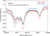 |
Fig. 11 Spectra of Venus between 529.65 and 529.85 cm−1 (18.9 µm) recorded on October 7, 2023 at the disk center (red points) and at 30°N latitude (blue points). Models: SO2(57 km) = 500 ppbv, SO2(62 km) = 400 ppbv. From top to bottom: SO2(67 km) = 0, 50, 100 and 200 ppbv. |
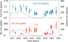 |
Fig. 12 Top: long-term variations in the disk-integrated H2O volume mixing ratio (blue points), inferred from the HDO measurements at the cloud top from the TEXES data at 7.4 µm. Bottom: long-term variations in the disk-integrated SO2 volume mixing ratio inferred at the cloud top (7.4 µm, red points). A daily value is shown in this figure. The error bars represent the uncertainty in the disk-integrated HDO and SO2 volume mixing ratios, averaged over a day. They depend upon the quality of the terrestrial atmospheric transparency, the size of the planetary disk, the continuum level and the number of maps recorded each day. In both cases, the solar activity (measured by the sunspot number) is shown for comparison. |
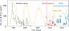 |
Fig. 13 Long-term variations in the SO2 volume mixing ratio measured at the cloud top between 1978 and 2025. The data prior to 2012 are taken from Esposito et al. 1984 (Pioneer Venus) and from Marcq et al. 2020 (Venus Express). They have been obtained in the UV, at an altitude of about 70 km, and the TEXES data have been normalized accordingly. The solar activity (measured by the sunspot number) is shown for comparison. |
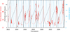 |
Fig. 14 Long-term variations in the SO2 volume mixing ratio measured by TEXES at the cloud top between 2012 and 2025 (red points). The Venus diameter (red line), the local time at the disk center (black line) and the longitude at the disk center (blue line) are shown for comparison. |
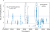 |
Fig. 15 Long-term variations in the SO2 (57 km)/SO2(62km) ratio between 2012 and 2025 (blue points), obtained from the disk-integrated SO2 mixing ratios derived at 7.4 µm (z = 62 km) and 18.9 µm (z = 57 km). |
5 Variation of the SO2 abundance as a function of local time
We have reconsidered our analysis of the SO2 variations at the cloud top as a function of the local time. As a reminder, our method consists in selecting one map per day and evaluating, on each map, the latitude, longitude and LT range of the SO2 plume (E23 and references therein). We then summed up all data from 2012 to 2022. Our previous study has shown that the SO2 plumes are mostly concentrated around the equator, while their distribution as a function of longitude has turned out to be inconclusive. For this reason, we concentrate here on the local time variations in SO2. Previous studies have shown that the probability of appearance of the SO2 plumes was apparently higher around the terminators (E23).
Figure 16 shows the probability of SO2 plume appearance (independent of the SO2 abundance) as a function of local time, using the whole dataset (2012–2025, 93 pts), and Figure 17 shows the SO2 distribution as a function of local time, which can be compared to Venus Express and Akatsuki observations. In the present study, we have also taken into account the fact that the SO2 abundance as a function of time might be driven by different mechanisms and we have isolated three data sets corresponding to three different periods. The first period includes the 2012–2017 data (27 points), for which the SO2 vertical gradient was relatively uniform (Fig. 15). The second period includes the data taken in 2021–2022 (28 points), when the SO2 abundance was especially low (Fig. 12 and 13). The last period is the most recent one (2023–2025, 17 points) which shows strong variations in the SO2 vmr.
It is interesting to note that the different data sets lead to significant differences. The probability of SO2 plume appearance shows, in all cases, a clear minimum around noon. Taking into account the whole data set, two maxima appear around 05:00 and 17:00, one hour before terminator. The SO2 vmr distribution shows even stronger differences between the different data sets. A maximum SO2 abundance appears in the afternoon (especially around 16:00) in 2012–2017, but there is no clear variation with local time in 2021–2022. In contrast, the last data set (2023–2025) exhibits a strong minimum around noon. These results are discussed in Section 6.
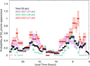 |
Fig. 16 Probability of SO2 appearance as a function of local time. Black: total (2012–2025, 93 points); violet: 2012–2017 (27 points); green: 2021–2022 (28 points); red: 2023–2025 (17 points). The error bar is proportional to n−0.5, where n is the number of observations for which the local time is observed. The local hour scale increases from right to left, corresponding to the orientation on the Venus disk as seen by an external observer. |
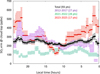 |
Fig. 17 Distribution of the SO2 vmr as a function of local time. Black: total (2012–2025 , 93 points); violet: 2012–2017 (27 points); green: 2021–2022 (28 points); red: 2023–2025 (17 points). The error bar is proportional to n−0.5, where n is the number of observations for which the local time is observed. The local hour scale increases from right to left, corresponding to the orientation on the Venus disk as seen by an external observer. |
6 Discussion and conclusions
6.1 The SO2 vertical distribution
When we started modeling the SO2 transitions at 7.4 and 18.9 µm, we soon realized that these lines were broader than the CO2 and HDO lines, which implied that a cutoff was needed in the SO2 vertical distribution a few kilometers above the clouds. In our latest calculations (E23), this cutoff, slightly depending on the thermal profile used, was fixed at z =70 km. The relations between the SO2/CO2 line depth ratios and the SO2 vmr were derived assuming this cutoff, and refer to the pressure levels of 100 mbar and 250 mbar, respectively.
The detection of the SO2 band at 8.6 µm introduces a new constraint in the SO2 vertical distribution. Figures 3–5 and 9–11 show that we have difficulties to fit the three spectra simultaneously, both in the case of disk-integrated and located spectra. They also illustrate that our determination of the SO2 vmr at z = 57 km and z = 62 km is model dependent, as the amplitude of the SO2 absorption at 7.4 and 18.9 µm depends upon the cutoff altitude assigned in our model. This means that the equations used in Section 3 to infer the HDO and SO2 volume mixing ratios are adequate in the case of HDO (because the H2O vmr appears to be constant with height in the altitude range probed by TEXES), but is model-dependent in the case of SO2, which exhibits significant variations as a function of altitude. Nevertheless, assuming for SO2 a constant altitude cutoff, as we did previously, allows us to determine what we call the SO2 vmr at 57 and 62 km, which we consider as representative indicators of the SO2 abundances at these altitudes. This simple method has allowed us to monitor the SO2 long-term evolution and to compare it to the temporal evolution of H2O. It has also allowed us to build maps of the two species over the Venus disk, which have revealed the existence of the SO2 plumes and have been used to monitor their short-term evolution.
Ideally, an inversion algorithm should be used to retrieve the H2O and SO2 vertical profiles. This analysis is beyond the scope of the present study, but will be considered in a future work. Here we limit ourselves to a few general comments. The strong modulation of the SO2 lines, in Figures 10 and 11, suggests that, at least in the two specific locations observed on October 7, 2025, SO2 is present above the cutoff level introduced at z = 72 km in our calculations. Another surprising feature is the very low SO2 vmr derived at z = 57 km at the disk center (Fig. 7). An inversion in the vertical profile of the SO2 vmr (being lower at 57 km than at 62 km), seems to be required to reconcile the data. It can be noted that this strange behavior is also observed in a few occasions on the disk-integrated SO2 vmr, especially in 2021–2023 (Fig. 15).
Another comment can be made about the parallel band structure observed on October 7, 2023. It can be seen from Figure 7 that the life time of this uncommon dynamical structure is exceptionally long, since it is continuously observed from October 3 to October 7, following the 4-day period rotation at the cloud top. In the past, we have seen only one example of a dynamical structure lasting more than a day, in November 7–9, 2021 (E23).
6.2 Long-term evolution of SO2 and H2O
Figures 12 and 13 illustrate the influence of the solar cycle on the long-term evolution of SO2 and H2O at the cloud top of Venus. In particular, the increase in the solar irradiance in 1978–1981 is likely to be responsible for the sharp decrease of the SO2 vmr which does not necessarily require episodic volcanic activity, as suggested previously by Esposito et al. (1984) and Marcq et al. (2013). The solar cycle also explains well the evolution of SO2 and H2O between 2012 and 2023. However, the sharp decrease of SO2 observed by Venus Express in 2006–2009 does not coincide with an increase in the solar activity, and the strong fluctuations of the SO2 vmr since 2023 remain a mystery. Theses anomalies suggest that other mechanisms are involved, possibly associated with dynamical motions, sublimation/condensation processes or SO2 gas-aerosol conversion.
6.3 SO2 distribution as a function of local time
The changes observed in the SO2 vmr distribution with local time between the three different period considered here (2012–2017, 2021–2022, 2023–2025, Fig. 17) could also be the signature of changes of regime. The SO2 maximum observed in the afternoon in 2012–2017 is in good agreement with the UV measurements of Akatsuki which probe a slightly higher altitude, at about 70 km (Iwanaka et al. 2025) which were taken in 2016–2022. It is also in good agreement with the global circulation models (Stolzenbach et al. 2023). However, this trend is no more visible in the TEXES data after 2021. In 2021–2022, the SO2 distribution as a function of local time is remarkably flat, while the 2023–2025 SO2 distribution shows a strong minimum around noon, in better agreement with the SPICAV/Venus Express data taken earlier (2006–2015; Marcq et al. 2020). This temporal evolution of the SO2 distribution as a function of local time is puzzling. It should be noted that the effects of local time and longitude are difficult to disentangle, and topographic effects (not considered in this analysis) could also possibly play a role in the SO2 distribution along the equator.
Data availability
The TEXES image cubes used in this paper are archived at the InfraRed Science Archive (IRSA), operated by the Infrared Processing and Analysis Center (IPAC) of the California Institute of Technology (https://irsa.ipac.caltech.edu/frontpage/) and can be downloaded at https://irsa.ipac.caltech.edu/applications/irtf/, specifying the Venus NAIF id 299 and the observing runs 2023A009 (March and July 2023), 2023B002 (October and December 2023), 2024A006 (February 2024), 2024B017 (January and March 2025). Data are available to the community after a 18-month proprietary period. The solar data are taken from the Solar Influences Data Analysis Center of the Royal Observatory of Belgium (https://sidc.be/SILSO/datafiles#total). The ephemeris are taken from the JPL Horizons system (https://ssd.jpl.nasa.gov/horizons).
Acknowledgements
TE, TKG and RG were visiting astronomers at the NASA Infrared Telescope Facility, which is operated by the University of Hawaii under Cooperative Agreement no. NNX-08AE38A with the National Aeronautics and Space Administration, Science Mission Directorate, Planetary Astronomy Program. We wish to thank the IRTF staff for the support of TEXES observations. This work was supported by the Programme National de Planétologie (PNP) of CNRS/INSU, co-funded by CNES. TKG acknowledges support of NASA Grant NNX14AG34G. TE and BB acknowledge support from CNRS. TW acknowledges support from the University of Versailles-Saint-Quentin and the European Commission Framework Program FP7 under Grant Agreement 606798 (Project EuroVenus). ML acknowledges funding from the European Union’s Horizon Europe research and innovation program under the Marie Sklodowska-Curie grant agreement 101110489/MuSICA-V. WS acknowledges support from China Scholarship Council Fellowship.
References
- Belyaev, D. A., Montmessin, F., Bertaux, J.-L., et al. 2012, Icarus, 217, 740 [CrossRef] [Google Scholar]
- Bézard, B., & DeBergh, C. 2012, J. Geophys. Res., 112, E04S07 [Google Scholar]
- Encrenaz, T., Greathouse, T. K., Richter, M. J., et al. 2013, Astron. Astrophys. 559, A65 [Google Scholar]
- Encrenaz, T., Greathouse, T. K., Giles, R., et al. 2023, Astron. Astrophys., 674, A199 [Google Scholar]
- Esposito, L. W. 1984, Science, 223, 1072 [Google Scholar]
- Esposito, L. W., Bertaux, J.-L., Krasnoposly, V., et al. 1997, Chemistry of lower atmosphere and clouds, in Venus II: Geology, Geophysics, Atmosphere, and Solar Wind Environment, eds. Bougher, S. W., Hunten, D. M., & Phillips, R. J., 415 [Google Scholar]
- Fedorova, A., Korablev, O., Vandaele, A.-C., et al. 2008, J. Geophys. Res., 113, E00B25 [Google Scholar]
- Giles, R., Greathouse, T. K., Irwin, P., et al. 2022, Icarus, 387, 115187 [NASA ADS] [CrossRef] [Google Scholar]
- Iwanaka, T., Imamura, T., Aoki, S., et al. 2025, JGR Planets, doi:10.1029/2024/E008775 [Google Scholar]
- Jacquinet-Husson, N., Scott, N., Chedin, A., et al. 2018, J. Quant. Spectr. Rad. Transfer 109, 1043 [Google Scholar]
- Krasnopolsky, V. A. 1986, Photochemistry of the atmospheres of Mars and Venus (New York: Springer Verlag) [Google Scholar]
- Krasnopolsky, V. A. 2007, Icarus, 191, 25 [NASA ADS] [CrossRef] [Google Scholar]
- Krasnopolsky, V. A. 2010, Icarus, 209, 314 [NASA ADS] [CrossRef] [Google Scholar]
- Krasnopolsky, V. A., Belyaev, D. A., Gordon, I. A., et al. 2013, Icarus, 224, 57 [NASA ADS] [CrossRef] [Google Scholar]
- Lacy, J. H., Richter, M. J., Greathouse, T. K., et al. 2002, Pub. Astron. Soc. Pac., 114, 153 [Google Scholar]
- Marcq, E., Bertaux, J.-L., Montmessin, F., et al. 2013, Nat. Geosci., 6, 25 [CrossRef] [Google Scholar]
- Marcq, E., Mills, F. P., Parkinson, C. P., & Vandaele, A. C. 2018, Space Sci. Rev., 214, 10 [NASA ADS] [CrossRef] [Google Scholar]
- Marcq, E., Jessup, K. L., Baggio, L., et al. 2020, Icarus, 335, 11368 [Google Scholar]
- Mills, F. P., Esposito, L. W., & Yung, Y. K. 2007, in Exploring Venus as a Terrestrial Planet, Geophysical Monograph Series, 176, 73 [CrossRef] [Google Scholar]
- Nakazawa, T., & Tanaka, M. 1982, J. Quant. Spect. Rad. Transfer, 28, 409 [Google Scholar]
- Parkinson, C., Gao, P., Esposito, L., et al. 2015, Plan. Space Sci., 112, 226 [Google Scholar]
- Rohlfs, K., & Wilson, T. L. 2004, Tools for Radioastronomy, 4th edn. (Berlin: Springer) [Google Scholar]
- Stolzenbach, A., Lefèvre, F., Lebonnois, S., et al. 2023, Icarus, 395, 115447 [NASA ADS] [CrossRef] [Google Scholar]
- Titov, D. V., Ignatiev, N. I., Mc Gouldrick, K., et al. 2018, Space Sci. Rev., 214, 126 [NASA ADS] [CrossRef] [Google Scholar]
- Vandaele, A.-C., Korablev, O., Belyaev, D., et al. 2017a, Icarus, 295, 16 [NASA ADS] [CrossRef] [Google Scholar]
- Vandaele, A.-C., Korablev, O., Belyaev, D., et al. 2017b, Icarus, 295, 1 [NASA ADS] [CrossRef] [Google Scholar]
- Zhang, K., Liang, M. C., & Mills, F. P. 2012, Icarus, 217, 714 [NASA ADS] [CrossRef] [Google Scholar]
- Zasova, L. V., Moroz, V. I., Esposito, L. W., & Na, C. Y. 1993, Icarus, 105, 92 [NASA ADS] [CrossRef] [Google Scholar]
All Tables
All Figures
|
Fig. 1 Examples of disk-integrated spectra of Venus (normalized radiance) recorded in 2023–2025. Left: 1344.85–1345.30 cm−1 spectral range (7.4 µm). The spectra are shifted by −0.2 in vertical scale for clarity. Right: examples of disk-integrated spectra of Venus (normalized radiance) between 529.65 and 529.85 cm−1 (18.9 µm). The spectra are shifted by −0.1 in vertical scale for clarity. |
| In the text | |
|
Fig. 2 Disk-integrated spectra of Venus between 1160 and 1163 cm−1 (8.6 µm) recorded on July 14, 2023, October 7, 2023 and January 22, 2025. The positions of the strongest SO2 lines are indicated in red by vertical dashed lines. The terrestrial lines coincide in the July 2023 and January 2025 because the Doppler shift is the same for both datasets, while it is different for the spectrum taken in October 2023. The spectra are dominated by terrestrial atmospheric absorption features, mostly N2O and O3. The black rectangle shows the spectral range used for our analysis. |
| In the text | |
|
Fig. 3 Disk-integrated spectrum of Venus between 1160.69 and 1160.80 cm−1 (8.6 µm) recorded on July 14. Models: SO2(57 km) = 500 ppbv, SO2(62 km) = 400 ppbv, SO2(67 km) = 50 ppbv (green), 100 ppbv (red) and 150 ppbv (blue). |
| In the text | |
|
Fig. 4 Disk-integrated spectrum of Venus between 1344.95 and 1345.25 cm−1 (7.4 µm) recorded on July 14, 2023. Models: SO2(57 km) = 500 ppbv, SO2(62 km) = 400 ppbv, SO2(67 km) = 0 ppbv (green), 100 ppbv (red) and 200 ppbv (blue). |
| In the text | |
|
Fig. 5 Disk-integrated spectrum of Venus between 529.65 and 529.85 cm−1 (18.9 µm) recorded on July 14, 2023. Models: SO2(57 km) = 500 ppbv, SO2(62 km) = 400 ppbv, SO2 (67 km) = 0 ppbv (green), 100 ppbv (red) and 200 ppbv (blue). |
| In the text | |
|
Fig. 6 Top: SO2 maps recorded on July 14, 2023. Left: z = 67 km (SO2 line depth); middle: z = 62 km (SO2/CO2 line depth ratio); right: z = 57 km (SO2/CO2 line depth ratio). Disk-integrated spectra corresponding to these maps are shown in Figs. 3–5. Bottom: continuum maps recorded on July 14, 2023 at z = 67 km (left), 62 km (middle) and 57 km (right). |
| In the text | |
|
Fig. 7 SO2 maps recorded on October 3–7, 2023. Left: z = 67 km (SO2 line depth); middle: z = 62 km (SO2/CO2 line depth ratio); next: z = 57 km (SO2/CO2 line depth ratio). Last right column: continuum maps recorded on October 3–7, 2023 at z = 62 km. The black crosses on the October 7 SO2 maps indicate the positions corresponding to the spectra shown in Figs. 9–11 (disk center and 30°N latitude). |
| In the text | |
|
Fig. 8 Top: SO2 maps recorded on January 22, 2025. Left: z = 67 km (SO2 line depth); middle: z = 62 km (SO2/CO2 line depth ratio); right: z = 57 km (SO2/CO2 line depth ratio). Bottom: continuum maps recorded on January 22, 2025 at z = 67 km (left), 62 km (middle) and 57 km (right). |
| In the text | |
|
Fig. 9 Spectra of Venus between 1160.75 and 1160.79 cm−1 (8.6 µm) recorded on October 7, 2023 at the disk center (red points) and at 30N latitude (blue points). Models: SO2(57 km) = 500 ppbv, SO2(62 km) = 400 ppbv. From top to bottom: SO2(67 km) = 50, 100 and 200 ppbv. |
| In the text | |
|
Fig. 10 Spectra of Venus between 1344.95 and 1345.25 cm−1 (7.4 µm) recorded on October 7, 2023 at the disk center (red points) and at 30°N latitude (blue points). Models: SO2(57 km) = 500 ppbv, SO2(62 km) = 400 ppbv. From top to bottom: SO2(67 km) = 0, 50, 100 and 200 ppbv. |
| In the text | |
|
Fig. 11 Spectra of Venus between 529.65 and 529.85 cm−1 (18.9 µm) recorded on October 7, 2023 at the disk center (red points) and at 30°N latitude (blue points). Models: SO2(57 km) = 500 ppbv, SO2(62 km) = 400 ppbv. From top to bottom: SO2(67 km) = 0, 50, 100 and 200 ppbv. |
| In the text | |
|
Fig. 12 Top: long-term variations in the disk-integrated H2O volume mixing ratio (blue points), inferred from the HDO measurements at the cloud top from the TEXES data at 7.4 µm. Bottom: long-term variations in the disk-integrated SO2 volume mixing ratio inferred at the cloud top (7.4 µm, red points). A daily value is shown in this figure. The error bars represent the uncertainty in the disk-integrated HDO and SO2 volume mixing ratios, averaged over a day. They depend upon the quality of the terrestrial atmospheric transparency, the size of the planetary disk, the continuum level and the number of maps recorded each day. In both cases, the solar activity (measured by the sunspot number) is shown for comparison. |
| In the text | |
|
Fig. 13 Long-term variations in the SO2 volume mixing ratio measured at the cloud top between 1978 and 2025. The data prior to 2012 are taken from Esposito et al. 1984 (Pioneer Venus) and from Marcq et al. 2020 (Venus Express). They have been obtained in the UV, at an altitude of about 70 km, and the TEXES data have been normalized accordingly. The solar activity (measured by the sunspot number) is shown for comparison. |
| In the text | |
|
Fig. 14 Long-term variations in the SO2 volume mixing ratio measured by TEXES at the cloud top between 2012 and 2025 (red points). The Venus diameter (red line), the local time at the disk center (black line) and the longitude at the disk center (blue line) are shown for comparison. |
| In the text | |
|
Fig. 15 Long-term variations in the SO2 (57 km)/SO2(62km) ratio between 2012 and 2025 (blue points), obtained from the disk-integrated SO2 mixing ratios derived at 7.4 µm (z = 62 km) and 18.9 µm (z = 57 km). |
| In the text | |
|
Fig. 16 Probability of SO2 appearance as a function of local time. Black: total (2012–2025, 93 points); violet: 2012–2017 (27 points); green: 2021–2022 (28 points); red: 2023–2025 (17 points). The error bar is proportional to n−0.5, where n is the number of observations for which the local time is observed. The local hour scale increases from right to left, corresponding to the orientation on the Venus disk as seen by an external observer. |
| In the text | |
|
Fig. 17 Distribution of the SO2 vmr as a function of local time. Black: total (2012–2025 , 93 points); violet: 2012–2017 (27 points); green: 2021–2022 (28 points); red: 2023–2025 (17 points). The error bar is proportional to n−0.5, where n is the number of observations for which the local time is observed. The local hour scale increases from right to left, corresponding to the orientation on the Venus disk as seen by an external observer. |
| In the text | |
Current usage metrics show cumulative count of Article Views (full-text article views including HTML views, PDF and ePub downloads, according to the available data) and Abstracts Views on Vision4Press platform.
Data correspond to usage on the plateform after 2015. The current usage metrics is available 48-96 hours after online publication and is updated daily on week days.
Initial download of the metrics may take a while.