| Issue |
A&A
Volume 703, November 2025
|
|
|---|---|---|
| Article Number | A245 | |
| Number of page(s) | 19 | |
| Section | Planets, planetary systems, and small bodies | |
| DOI | https://doi.org/10.1051/0004-6361/202556346 | |
| Published online | 24 November 2025 | |
Stellar-activity analysis of the nearby M dwarf GJ 526
Multi-dimensional Gaussian-process modelling of RV, FWHM, and S-index
1
Instituto de Astrofísica de Canarias, 38205 La Laguna, Spain
2
Departamento de Astrofísica, Universidad de La Laguna, 38206 La Laguna, Spain
3
Consejo Superior de Investigaciones Científicas (CSIC), 28006 Madrid, Spain
4
Light Bridges S. L., 35004 Las Palmas de Gran Canaria, Spain
5
Dipartimento di Fisica e Astronomia “Galileo Galilei”, Università di Padova, Vicolo dell’Osservatorio 3, 35122 Padova, Italy
6
Instituto de Astrofísica e Ciências do Espaço, CAUP, Universidade do Porto, Rua das Estrelas, 4150-762 Porto, Portugal
7
Departamento de Física de la Tierra y Astrofísica & IPARCOS-UCM (Instituto de Física de Partículas y del Cosmos de la UCM), Facultad de Ciencias Físicas, Universidad Complutense de Madrid, 28040 Madrid, Spain
8
Centro de Astrobiología (CAB), CSIC-INTA, ESAC campus, Camino Bajo del Castillo s/n, 28692 Villanueva de la Cañada, Spain
9
Observatoire Astronomique de l’Université de Genève, Chemin Pegasi 51b, 1290 Versoix, Switzerland
10
Departamento de Física e Astronomia, Faculdade de Ciências, Universidade do Porto, Rua do Campo Alegre, 4169-007 Porto, Portugal
11
INAF – Osservatorio Astrofisico di Torino, Via Osservatorio 20, 10025 Pino Torinese, Italy
12
INAF – Osservatorio Astrofisico di Trieste, via G. B. Tiepolo 11, 34143 Trieste, Italy
13
IFPU – Institute for Fundamental Physics of the Universe, via Beirut 2, 34151 Trieste, Italy
14
Centro de Astrofísica da Universidade do Porto, Rua das Estrelas, 4150-762 Porto, Portugal
★ Corresponding author: This email address is being protected from spambots. You need JavaScript enabled to view it.
Received:
10
July
2025
Accepted:
2
September
2025
Abstract
M dwarfs are the most abundant stars in the Galaxy, and their low masses make them natural favourites for exoplanet radial-velocity (RV) searches. Nevertheless, these stars often demonstrate strong stellar activity that is yet to be fully understood. We used high-precision ESPRESSO, HIRES, and HARPS spectroscopy to perform a stellar-activity analysis on the nearby early M dwarf GJ 526 (d = 5.4 pc). We carried out a joint modelling of (i) the stellar rotation in RV, full width at half maximum (FWHM), and Mount Wilson S-index through Gaussian processes; (ii) long-term trends in these three physical quantities; and (iii) RV planetary signals. We constrained the stellar-rotation period to Prot = 48.7 ± 0.3 d, and discovered a weak sinusoidal signature in RV, FWHM, and S-index of period Pcyc = 1680−40+50d. We propose phase-space trajectories between RV and activity indicators as a novel means to visualise and interpret stellar activity. Current evidence does not support planetary companions of GJ 526.
Key words: techniques: radial velocities / stars: activity / stars: low-mass / stars: individual: GJ 526
© The Authors 2025
 Open Access article, published by EDP Sciences, under the terms of the Creative Commons Attribution License (https://creativecommons.org/licenses/by/4.0), which permits unrestricted use, distribution, and reproduction in any medium, provided the original work is properly cited.
This article is published in open access under the Subscribe to Open model. This email address is being protected from spambots. You need JavaScript enabled to view it. to support open access publication.
1 Introduction
M dwarfs, the most prevalent stars in the Galaxy, remain very attractive for exoplanetary radial-velocity (RV) detection due to their low masses. In practice, however, M dwarfs stubbornly mask potential planetary RV signals through physical processes such as stellar activity on both short and long timescales (Borgniet et al. 2015 and Dumusque et al. 2011, respectively). To compound the situation, M-dwarf activity is sometimes exhibited at periods that overlap with the habitable zone of potential planetary companions (e.g. GJ 15A; Pinamonti et al. 2018). It is therefore important to understand better how stellar activity affects RV measurements, so as to improve our ways of detection.
In this work, we examined the RV behaviour of one such M dwarf, GJ 526 (α = 13h45m43.8s, δ = 14°53′29.5″; Gaia Collaboration 2022, hereafter GDR3). This nearby star has been known to the scientific community since the beginning of the nineteenth century at the latest (de Lalande 1801). Its close proximity to the Sun was identified at least since Porter (1892) measured its extraordinarily large proper motion. At present, the distance to GJ 526 is well constrained to 5.435 pc (GDR3), but its stellar parameters are moderately established. GJ 526 is thought to have a spectral class between M1 and M2 (Rojas-Ayala et al. 2012; Gaidos et al. 2014); recently, Passegger et al. (2022) computed standardised stellar parameters and reported an effective temperature Teff = 3648 ± 88 K and a surface gravity log g = 4.75 ± 0.04, in combination with past measurements in the literature (see references therein). GJ 526 exhibits a particularly slowly evolving and foreseeable activity, which made it an attractive choice for a spectral standard in studies of various nature (e.g. Binks & Jeffries 2016; Martinez et al. 2017; Pancino et al. 2017; Fuhrmeister et al. 2019). Its stellar rotation is revealed by periodic signatures in both RV and activity data; Suárez Mascareño et al. (2017), hereafter SM17, identified a strong RV signal at 49.2 ± 0.1 d and constrained the stellar-rotation period to 52.1 ± 12.0 d.
GJ 526 has been studied by several RV programmes, including the Lick Planet Search Program (hereafter Lick; Fischer et al. 2014), HIRES (Vogt et al. 1994), HARPS (Mayor et al. 2003), CARMENES (Quirrenbach et al. 2016), and ESPRESSO (Pepe et al. 2014, 2021), in this order. The combination of these surveys has provided 26 yr velocimetry, which includes high-precision measurements from the ultra-stable ESPRESSO spectrograph, with a typical photon-noise uncertainty near 10cm s−1. Even though all the aforementioned sources provide rich and multifaceted data, there has been no evidence of planetary companions of GJ 526 to date. This work continues as follows. Section 2 describes the observational data relevant to our study. Section 3 contains our derivation of stellar parameters for GJ 526. Section 4 reviews our modelling approach, Section 5 looks into the results of our models, and Section 6 discusses their implications. We summarise our work in Section 7.
2 Observations
2.1 ESPRESSO velocimetry
ESPRESSO is a high-resolution ultra-stable échelle spectrograph. It is located at the ESO Very Large Telescope, Paranal Observatory, Chile, and it can be fed with signal from just one or from all the 8.2 m unit telescopes of the facility (Pepe et al. 2014, 2021). This spectrograph was designed to reach an RV precision of 10cm s−1, allowing Earth-like planets to be detected in the habitable zones of GKM dwarfs. ESPRESSO already achieves an RV precision of 25cm s−1 over the course of a night and 50cm s−1 over the course of months. In fact, Pepe et al. (2021) suggests an instrumental precision of 10cm s−1, leaving aside photon-noise and stellar-jitter limits. We acquired 75 ESPRESSO measurements of GJ 526 as part of its Guaranteed Time Observations (GTO)1. In nine measurements, the atmospheric dispersion corrector of ESPRESSO malfunctioned, which led to a non-quantified error in velocimetry2. We removed them and continued with the 66 remaining measurements. ESPRESSO RVs were extracted from the spectra through the cross-correlation function method (CCF method; Baranne et al. 1996), and through its own Data Reduction Software (DRS), version 3.2.5.
Our data span from February 2019 to March 2023, with a median interval of 6.0 d between measurements. This temporal coverage includes the June 2019 fibre link change, which introduced an RV offset in measurements (Pepe et al. 2021). This led some works to regard the ESPRESSO data as two separate datasets: before and after the fibre link (e.g. Faria et al. 2022; Suárez Mascareño et al. 2023). We also followed this procedure, and hereafter label these datasets as ESPRESSO18 (N = 14) and ESPRESSO19 (N = 52). The two subsets have a similar RV root mean square (rms) and median uncertainty. ESPRESSO18 is characterised by an RV rms of 2.49 m s-1 and a median uncertainty of 0.13ms−1, while ESPRESSO19 has an RV rms of 2.20 m s−1 and a median photon-noise uncertainty of 0.14 m s−1.
2.2 HARPS velocimetry
HARPS is a high-resolution échelle spectrograph located at the 3.6 m telescope, ESO, La Silla, Chile, and was the first spectrograph to break the 1 m s−1 barrier in RV precision (Mayor et al. 2003). We made use of the public HARPS RV database by Trifonov et al. (2020) that contains 32 HARPS measurements of GJ 526, spanning from May 2005 to June 2009. All of these were acquired before the optical fibre update in May 2015. Two spectroscopic measurements were excluded on account of failing an iterative 3σ clipping criterion in FWHM. Then, the first and the last point of this intermediate dataset were separated by 310 d and 1845 d from the bulk of measurements (i.e. 21% and 125% relative to the bulk baseline). We chose to mask those out. This procedure yielded 28 spectroscopic measurements that span from May 2005 to June 2009, with a median interval of 3.1 d between measurements. Our HARPS data extend the baseline nicely, and have a median RV uncertainty of 0.62 m s−1.
2.3 HIRES velocimetry
HIRES is a high-resolution échelle spectrograph located at the 10 m Keck telescope, Mauna Kea Observatory, HI, USA (Vogt et al. 1994), and was initiated in 1994 as a search for exoplanets targeted around F, G, K, and M dwarfs. Butler et al. (2017) contains 56 HIRES measurements of GJ 526 that span from April 1997 to January 2014, with a median interval of 79 d between measurements. We used the systematic-corrected variant of this dataset, provided by Tal-Or et al. (2019). Their RV data have an rms of 3.43 m s−1 and a median uncertainty of 1.61 ms−1.
2.4 CARMENES velocimetry
CARMENES is a high-resolution échelle spectrograph located at the 3.5 m telescope at the Calar Alto Observatory, Spain, that was specially designed to search for planetary signatures around nearby, cool stars (Quirrenbach et al. 2014, 2016). There are 253 measurements of GJ 526 in the CARMENES Data Release 1 (Ribas et al. 2023), spanning from January 2016 to April 2018, with a median interval of 1.0 d between measurements, and a median RV uncertainty of 1.51 ms−1. We were unable to meaningfully work with these data, and it became necessary to exclude them from analysis. We describe the features of the CARMENES data and the issues we encountered with them in Sect. 5.3.2.
2.5 Lick velocimetry
The Lick programme was carried out with the Hamilton Spectrograph and the 3 m Shane telescope at the Lick Observatory, CA, USA (Fischer et al. 2014). The programme ran from 1987 to 2011 and supplied data that were fundamental to our current understanding of exoplanets (Marcy & Butler 1996; Butler et al. 1997, 1999). The Lick programme contains 16 RV measurements of GJ 526 from August 1992 to February 1997, with a median interval of 73 d between them. This dataset is characterised by large RV uncertainties, with a median of 21.21 ms−1. While we acknowledge the historical significance of the programme, such uncertainties are incompatible with the purposes of our study. This led us to exclude this dataset from our analysis.
2.6 Activity indicators
Active regions perturb the flux and velocity fields of the stellar disc, thereby changing the shape of observed lines. Consequently, the CCF also changes shape. Such perturbations are quantified by tracking the evolution of CCF width, depth, and symmetry; and their strength can be related to the coverage of the active regions, their contrast, and the stellar v sin i. In this work, we use the CCF full width at half maximum (CCF FWHM) as one of our main activity indicators. Two of the discussed datasets provide the CCF FWHM time series: ESPRESSO and HARPS. The ESPRESSO18 data are characterised by an FWHM rms of 2.99ms−1 and a median uncertainty of 0.26ms−1. For ESPRESSO19, those values stand at 8.15 ms−1 and 0.29ms−1 respectively. The HARPS FWHMs come with an rms of 4.49 ms−1 and a median uncertainty of 1.23 ms−1.
The emission intensity of the cores of Ca II H&K lines is a reliable proxy of the strength of the stellar magnetic field, and thereby of the stellar-rotation period Prot for late-type stars (Noyes et al. 1984; Lovis et al. 2005). We use the Mount Wilson S-index
 (1)
(1)
where ÑH and ÑK are triangular passbands centred at 3968.470 Å and 3933.664 A, with a common FWHM of 1.09 A; while ÑV and ÑR are rectangular passbands centred at 3901.07 A and 4001.07 A, with a common width of 20 A (Vaughan et al. 1978). Three discussed datasets provide the CCF S-index: ESPRESSO, HARPS, and HIRES. ESPRESSO18 is characterised by an Sindex rms of 40.4 × 10⁻³ and a median uncertainty of 0.14 × 10⁻³. For ESPRESSO19, those values stand at 125 × 10−3 and 0.17 × 10⁻³, respectively. Our HARPS measurements have an Sindex rms of 56.9 × 10⁻³ and a median uncertainty of 0.11 × 10⁻³, similar to both ESPRESSO18 and ESPRESSO19. Our HIRES Sindex measurements have an rms of 95.8 × 10⁻³, but came with no uncertainties; we assumed an uncertainty equal to the median in HARPS (0.11 × 10⁻³).
2.7 ASAS-SN, ASAS, and TESS photometry
ASAS-SN is an automated photometric programme that searches for supernovae and other transient events (Shappee et al. 2014; Kochanek et al. 2017). It is comprised of 24 ground-based 14 cm telescopes that are grouped in fours at six sites. ASAS was a programme that aimed to perform photometric monitoring over a large sky area (Pojmanski 1997), and its primary goal was to discover and catalogue variable stars of all kinds. TESS is a red-infrared all-sky survey that was specifically designed to detect exoplanetary transits and that continues to deliver precise long-term photometry (Ricker et al. 2015). The mission satellite utilises four wide optical cameras, each of which covering a solid angle of 24 deg × 24 deg. We give a short self-contained photometry analysis in Appendix A. Its key takeaway is that we found no signals we could attribute to stellar activity, except a 1333 d signal that we associated with the magnetic-cycle period Pcyc.
3 Stellar parameters
We derived the effective temperature Teff, the surface gravity log g, and the stellar metallicity [Fe/H] through STEPARSYN3 (Tabernero et al. 2022). We report the following measurements: Teff = 3699 ± 16 K, log g = 4.69 ± 0.05, [Fe/H] = −0.33 ± 0.07 dex, as well as the total line-broadening velocity vbroad = 2.26 ± 0.21 km s−1. For the STEPARSYN analysis, we used the line list and model grid described in Marfil et al. (2021). The stellar radius and mass were derived from the spectroscopic log g and from the linear mass-radius relation in Schweitzer et al. (2019). We report the following: M = 0.505 ± 0.058 M⊙, R = 0.479 ± 0.055 R⊙. Table 1 gives a complete list of stellar parameters.
We cross-checked our Teff, log g, and [Fe/H] results through ODUSSEAS4 (Antoniadis-Karnavas et al. 2024) on the combined high-resolution ESPRESSO spectra. The trigonometric surface gravity for this star was derived using recent GDR3 data and following Sousa et al. (2021). This derivation yielded the following: Teff = 3656 ± 92 K, log g = 4.67 ± 0.09, [Fe/H] = −0.242 ± 0.111 dex. These measurements are all consistent with our primary stellar-parameter derivation.
We validated our derivations of M, R, and the bolometric stellar luminosity L by computing the photometric spectral energy distribution (SED) of GJ 526 using the publicly available broad-band photometry from the following catalogues: GALEX (Bianchi et al. 2017), TYCHO (Høg et al. 2000), PanSTARRS (Chambers et al. 2016), SDSS (York et al. 2000), GDR3, 2MASS (Cutri et al. 2003), WISE (Wright et al. 2010), IRAS (Beichman et al. 1988), and AKARI (Ishihara et al. 2010). We used the photometric zero points listed in the Virtual Observatory SED Analyzer tool (VOSA; Bayo et al. 2008) to convert the observed magnitudes into fluxes, and the GDR3 trigonometric parallax to transform from observed to absolute fluxes. Figure B.1 compares the aforementioned photometric data against a PHOENIX model for solar metallicity and 3700 K (Allard et al. 2012). This fit agrees with the data, with the exception of the GALEX datapoint, which is the bluest photometric point. This suggests that GJ 526 is an active star. We then integrated the observed SED, excluding the GALEX datapoint, and obtained L = 0.0401 ± 0.0027 L⊙. Together with our derived Teff = 3699 ± 16 K from STEPARSYN, we derived R = 0.487 ± 0.029 R⊙ through the Stefan-Boltzmann law. The mass-radius relation of Schweitzer et al. (2019) suggests a stellar mass of M = 0.490 ± 0.030 M⊙. The computed surface gravity from these mass and radius values (log g = 4.753 ± 0.024) agree with our own spectroscopic derivation (log g = 4.69 ± 0.09). Finally, the mass-K-band luminosity relationship of (Mann et al. 2019) returned M = 0.483 ± 0.026 M⊙ for GJ 526, again in good agreement with our derivation.
The ESPRESSO spectra delivered log10 R′HK with a median value of −5.286, an rms of 0.087, and a median instrumental uncertainty of 1.2 × 10⁻⁴. We took the mean and the rms, and reported it in Table 1. Through the relation in Suárez Mascareño et al. (2018), our log10 R′HK translates to a stellar-rotation period of Prot = 51 d, a value that is consistent with our results to follow (Prot = 48.7 ± 0.3 d; Sect. 6.1)
Stellar parameters of GJ 526.
4 Modelling and inference
We used the modelling framework described in Stefanov et al. (2025), hereafter S25, that is generalised for N data sources (e.g. HIRES, HARPS; i ∈ [0..N - 1]) and M physical quantities (e.g. RV, FWHM; j ∈ [0..M - 1]). The S25 framework includes (i) long-term functions (LTFs) for data that follow physical or instrumental trends, (ii) offsets between different sources, (iii) source-dependent jitters for each quantity, (iv) Keplerian-and circular-orbit fitting, and (v) stellar-activity modelling using Gaussian processes. A brief discussion of the last step follows.
Gaussian processes (GPs) are collections of random variables, any finite number of which follow a joint Gaussian distribution (Rasmussen & Williams 2006). GPs are non-parametric models, meaning that the datasets themselves determine the functional form of the model. Instead, we feed to the GP certain functional relationships that are assumed to describe the correlations between individual measurements. For this reason, GPs are useful devices in the toolbox of planet-detection researchers as they require no other assumptions of the active regions that the star may exhibit (Haywood 2015).
Stellar activity is often modelled under the assumption that correlations between measurements are sensitive to a certain period - the stellar-rotation period - and at the same time, that correlations diminish exponentially at a certain timescale. These two assumptions motivate the squared-exponential periodic (SEP) kernel5, which has the form
![Mathematical equation: k_\text{SEP}(\Delta t) = \kappa^2\exp\left[ -\frac{\Delta t^2}{2\tau^2} -\frac{\sin^2\left(\pi\Delta t/P\right)}{2\eta^2} \right],](/articles/aa/full_html/2025/11/aa56346-25/aa56346-25-eq4.png) (2)
(2)
where κ2 is the maximum amplitude of the kernel, τ is the timescale of coherence, P is associated with the stellar-rotation period Prot, and η describes the kernel-feature complexity (Haywood et al. 2014; Rajpaul et al. 2015; Angus et al. 2018). We refer to η as the ‘sinescale’ on account of its algebraic analogy to the timescale τ. Invoking the SEP kernel directly comes with a computational overhead, and we work with two of its approximations: the Matérn 3/2 exponential periodic (MEP) kernel and the exponential-sine periodic (ESP) kernel, both as introduced in the S+LEAF6 library (Delisle et al. 2020, 2022).
Real-data experience shows that conditioning GP kernels onto RV data alone may cause the model to incorrectly address planetary signals as stellar activity, and therefore hinder planet detections. An emerging way to combat this is to fit GP-based models on RV and activity-indicator data, i.e. in several dimensions at the same time. By informing the GP kernel of the activity-indicator behaviour of the star, we allow that kernel to better separate planetary from non-planetary signals in RV (Ahrer et al. 2021; Rajpaul et al. 2021). In the case of GJ 526, we worked with RV, FWHM, and S-index at the same time. We followed the notation of S25, and assigned j = 0 for RV, j = 1 for FWHM, and j = 2 for S-index.
There are different ways to assign GPs to several physical quantities. One of them, the multi-dimensional regime, follows the FF′ formalism that was defined in Aigrain et al. (2012) and extended in Rajpaul et al. (2015). In this regime, one GP kernel is fitted on all physical quantities at the same time. For measurements yi,j at times ti,j, we solve the system of equations
![Mathematical equation: \left|\begin{array}{l} y_{i,j}=A_j\,G(t_{i,j})+B_j\,(\mathrm{d}G/\mathrm{d}t)_{t=t_{i,j}}\\[0.2ex] \shortvdots \end{array}\right.\qquad \begin{array}{l} \forall\, i, \\ \forall j, \end{array}](/articles/aa/full_html/2025/11/aa56346-25/aa56346-25-eq5.png) (3)
(3)
where Aj and Bj are quantity-specific fit hyperparameters, and G(ti,j) is the kernel estimation of the stellar activity at given times. The multi-dimensional regime is a common approach for the disentanglement of stellar activity in the velocimetry of late-type dwarfs (Barragán et al. 2023; Passegger et al. 2024), and it is useful to break degeneracies in cases where there is a significant correlation between physical quantities (Suárez Mascareño et al. 2020). Rajpaul et al. (2015) discussed how the FF′ formalism expects only some physical quantities to have non-zero Bj terms in (3); we refer to these as ‘gradiented’ with respect to the remaining quantities. We used the S+LEAF MultiSeriesKernel procedure to realise this regime.
4.1 Parameter priors
We used a set of default parameter priors across models unless stated explicitly. Our default LTF parameter priors are informed by the solutions of the Levenberg-Marquadt algorithm (LMA; Levenberg 1944; Marquardt 1963). We ran an instance of the LMA that returns a mean μ1m and an uncertainty σ1m for each LTF parameter. For these parameters, we then used the priors 𝒩 (μ1m, 200σ1m). The large scale factor of σ1m accounts for the minute errors that the LMA tends to return.
Our default offset priors are based on the common standard deviation of all yi,j, which we denote σj. The default prior on offsets is Oi,j = 𝒩(0,5σj). For jitters, we use the non-restrictive Ji,j = 𝒰log(10−3,103), except for RV jitters, where we take the log-normal distribution Oi,0 = exp [𝒩(ln σ0, ln σ0)], following González Hernández et al. (2024). In terms of SEP kernel hyperparameters, we use timescale priors of 𝒰log(20,104)d, period priors of 𝒰(40.1, 64.1)d as informed by SM17 (52.1 ± 12.0d), sinescale priors of 𝒰log(10−2,102), and the following amplitudes: A0, B0 = 𝒰(−10−3,103) for GP RV amplitudes, and Aj = 𝒰log(10−3,103) for GP indicator amplitudes.
4.2 Inference
Skilling (2004) noted that while directly sampling from the likelihood function L is exponentially more expensive, sampling uniformly within a bound L > k is much easier; increasing k iteratively upon reaching convergence can be used to evaluate the posterior. This strategy is now known as nested sampling. Its formalism allows it to have (i) lower computational complexity, (ii) the ability to explore multi-modal distributions of arbitrary complex shapes, and (iii) the ability to numerically evaluate the Bayesian evidence Z. We used ReactiveNestedSampler, a nested-sampling integrator provided by ULTRANEST7 (Buchner 2021). In every inference instance of Nparam model parameters, we required 40Nparam live points and a region-respecting slice sampler that accepted 4Nparam steps until the sample was considered independent.
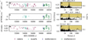 |
Fig. 1 Time series of mean-subtracted (a) RV, (c) FWHM, (e) S-index. The measurements are marked according to the data source: pink downward triangles for HIRES, teal upward triangles for HARPS, blue circles for ESPRESSO18, and green squares for ESPRESSO19. (b,d,f) Associated wide-period GLSPs of RV and activity indicators. Three FAP levels: 10%, 1%, and 0.1%, split GLSP ordinates in bands of different colours. We highlight the three most prominent peaks in each GLSP. |
5 Analysis
5.1 Features of available velocimetry
Figure 1 shows the generalised Lomb-Scargle periodograms (GLSPs; Lomb 1976; Scargle 1982; Zechmeister & Kürster 2009; VanderPlas & Ivezic 2015) of RV and all activity indicators in the period range 2-6000 d. RV data seem to be devoid of long-term trends. The GLSPs of FWHM and S-index, on the other hand, reveal significant periodicities near 1400 d in both physical quantities (Figs. 1d,f). This may be indicative of a magnetic cycle, and as such, it calls to be potentially included in the LTFs of our chosen models.
At shorter periods, we observe a distinct 48-49 d signal in RV and both activity indicators. This matches the stellar-rotation period measured by SM17 (Prot = 52.1 ± 12.0 d), and we likewise associate it with Prot. There are other signals in its company, most notably (i) a 3-4 d signature in RV, FWHM, and S-index; (ii) a forest of peaks extending up to 10 d in S-index; and (iii) a 63 d signature in RV and FWHM. A priori, we expect that these may be aliases of Prot, which come from the harmonic combination of Prot and any significant window-function (WF) peak at Pwf through the relation
 (4)
(4)
as described in Dawson & Fabrycky (2010). Therefore, by identifying the dominant WF peaks, we can check for aliases of Prot.
HIRES provides RV and S-index data, but not FWHM. Consequently, the WF formed by FWHM measurements is not equivalent to the WF that RV and S-index time series share. Although the timestamps of HIRES measurements certainly relocate powers in the WF, we verified that the first few WF peaks change marginally with the inclusion of HIRES points. We continued with the WF formed by HIRES, HARPS, and ESPRESSO to select alias-inducing peaks. Figure B.2 visualises our alias analysis. We identified four definite WF peaks that inject aliases of Prot. Those WF peaks are located at 215 d, 365 d, 477 d, and 657 d (Fig. B.2g). For Prot, they would generate aliases between 30-70 d. We observed that these WF peaks indeed generate aliases that match the observed structures, including the 0.1% FAP 63 d in RV, FWHM, and S-index (Figs. B.2a-c, teal upward triangle). A small peak between 30-40 d is also identified as an alias in all dimensions. The forest of signatures between 1-10 d remains unidentified in all physical quantities.
5.2 Long-term function selection
What remains to be verified is whether the 1400 d signals proposed by the FWHM and the S-index GLSPs are statistically significant. This can be checked through a suite of intermediate models that fit different LTFs to one-dimensional time series, without including any GPs. We prepared models that incorporate a polynomial function of degree pj ≤ 2 with respect to time, as well as a potential sinusoidal term. The full form of this general LTF is
![Mathematical equation: f_j(t_{i,j}) = \sum_{n=0}^{p_j} \alpha_n t^n_{i,j} + k_{\text{cyc, }j} \sin\left[\ \frac{2\pi(t_{i,j}+P_\text{cyc}\,\varphi_{\text{cyc, }j})}{P_\text{cyc}} \right],](/articles/aa/full_html/2025/11/aa56346-25/aa56346-25-eq7.png) (5)
(5)
where fj is the LTF as defined in S25; kcyc, j and φcyc, j are the cycle amplitude and cycle phase; and Pcyc is the cycle period8. We used a cycle-period prior of 𝒰log(200,104)d. For models with a sine-free LTF, we set kcyc,j = 0 and excluded the parameters of this term from sampling.
Zero-order polynomial LTFs scored best among all dimensions in terms of Bayesian evidence. This matches the lack of signals beyond 4000 d in GLSPs (Figs. 1b,d,f). The inclusion of a sine term in the LTF is favoured in FWHM (Δ ln Z = 2.8) and in S-index (Δ ln Z = 4.7). These intermediate models successfully recover a 1380 d FWHM signal of amplitude 4.59 m s−1, and a 1350
 d S-index signal of amplitude (5.77
 ) × 10−2. The phase posteriors from these two models hint that the two signals may be in phase (0.70
 in FWHM, 0.73
 in S-index). The agreement of these solutions with the 1400 d peaks in the GLSPs and the Δ ln Z improvement from their non-sine counterparts steers us towards a global zero-order LTF with a sine term.
5.3 Model selection
Having gained the insights described in Sect. 5.2, we adopted the LTF
![Mathematical equation: f_j(t_{i,j}) = \alpha_i + k_{\text{cyc, }j} \sin\left[\ \frac{2\pi(t_{i,j}+P_\text{cyc}\,\varphi_{\text{cyc, }j})}{P_\text{cyc}} \right].](/articles/aa/full_html/2025/11/aa56346-25/aa56346-25-eq13.png) (6)
(6)
We used the following LTF priors: a sine-term period of Pcyc = 𝒰(1000, 2000) d, and the following semi-amplitudes: kcyc,0 = 𝒰(0,10) m s−1 in RV, kcyc,1 = 𝒰(0,10)ms−1 in FWHM, and kcyc,2 = 𝒰(0,0.1) in S-index. Then we built a grid of multidimensional GP models that fit in all three physical quantities. This model grid probed different stellar-activity kernels, as well as different planetary configurations. For stellar activity, we used four different approximations of the SEP kernel: MEP, as well as ESP with two, three, and four harmonics (hereafter ESP2, ESP3, and ESP4). The ranks of these kernels increase in this order, and they can be assumed to grow likewise in complexity. In the design of planetary configurations, we either modelled for no planets or for a single circular-orbit planet. This gave a grid of eight different models. In all models, we used the multidimensional regime, with only RV being gradiented relative to FWHM and S-index. We used the default parameter priors as described in Sect. 4.1. For the modelled planet, we adopted an uninformed orbital-period prior of Pb = 𝒰log(1,1000) d and an amplitude prior of krv, b = 𝒰(0,5) m s−1.
Figure 2 displays a ln Z comparison of entries throughout our model grid. Entries are arranged so that planetary-system complexity increases downwards and stellar-activity complexity increases rightwards. The MEP kernel is widely endorsed in the model grid, with an average improvement in evidence of (Δ ln Z)avg > 5.4 relative to ESP kernels. The inclusion of a single circular-orbit planet is not favoured much by the data. We report an average improvement in evidence of (Δ ln Z)avg = 1.8 across all kernels; the largest improvement is Δ ln Z = 2.5 for the ESP4 kernel. We thereby select the most appropriate (‘best’) model in our analysis: the MEP planet-free model. What now follows is a discussion of the best-model fit and a brief comparison with similar models in our grid. We cover the implications of the best-model results in Sect. 6.1.
Our combined dataset of HIRES, HARPS, and ESPRESSO offers a very dissimilar temporal sampling. There are clusters of dozens of points within a few hundred days, as well as measurement gaps over several years. Although this uneven sampling is expected to challenge the GP framework, we observe a sound prediction in all physical quantities in the full baseline, as well as in clusters of densely sampled points. Figure B.3 displays the prediction of our best model (an LTF and a GP) against all raw time series. We observe stable structures, and no significant residual signals in any dimension. Figure 3 displays the same prediction, but in two selected densely sampled 240 d intervals: Interval A (approximately 2 458 504-2 458 744 BJD), and Interval B (approximately 2 459 219-2 459 459 BJD), both with 0.1 d prediction sampling. The MEP kernel models all measurements reasonably well, except for a few RV points in ESPRESSO18 (Fig. 3a). All O-C diagrams reveal residuals that are well distributed around the zero, with a spread similar to the assigned model jitters. We report the following residual rms against the median ‘jittered’ uncertainties: 1.46ms−1 against 1.89ms−1 in RV, 2.57ms−1 against 1.85ms−1 in FWHM, and 29 × 10−3 against 33 × 10−3 in S-index. We list the posterior of our best model in Table B.1, in the column ‘All-data’. All posteriors were well-behaved in shape and did not appear to be biased by the prior space we imposed. We discuss the meaning of these results in Sect. 6.1.
We compared our best model with other planet-free models in our model grid (Fig. 2), that is, against the ESP2, ESP3, and ESP4 models. Table B.2 lists the posteriors of the four aforementioned models. We report marginal differences between all posteriors overall, with the exception of a larger timescale in MEP (τ = 277 d) than in ESP kernels: 68
 d in ESP2, 79
 d in ESP3, and 81
 d in ESP4. This difference might come from how τ enters algebraically into the MEP and the ESP kernels (see Delisle et al. 2022). While our best model assigned a larger τ uncertainty compared to its ESP counterparts, it constrained the stellar-rotation period Prot better. We report Prot = 48.7 ± 0.3 d in MEP, against 49.2
 d in ESP2, 49.2
 d in ESP3, and 49.3
 d in ESP4.
Then, we took our best model, and reduced it to two twodimensional partitions: RV & FWHM and RV & S-index. Albeit with marginally noisier posteriors, these two partitions remained potent in the modelling of stellar activity. We report the following stellar-rotation period and timescale for the RV & FWHM and RV & S-index respectively: 48.8 d and 48.7
 d for Prot, as well as 353
 d and 147
 d for τ. Other partition-model parameters have a similar posterior to those from our best model, with the exception of the LTF period, where partition models assigned up to two secondary modes in the 𝒰(1000,2000) d prior.
Finally, we used S-BART9 (Silva et al. 2022) on the ESPRESSO and HARPS data in order to self-validate our results under a different reduction framework. We reduced all available raw ESPRESSO and HARPS spectra through S-BART, and from there we took only RVs and their associated uncertainties. Then, we cross-matched our dataset with S-BART RVs by time, thereby rejecting the same outliers. We report the following rms and median uncertainty of S-BART RVs: 2.37 m s−1 and 0.09ms−1 for ESPRESSO18, 2.35ms−1 and 0.10ms−1 for ESPRESSO19, and 2.41ms−1 and 0.51 m s−1 for HARPS. We ran a duplicate of our best model, though with S-BART RVs.
We found no differences from our best-model results (Table B.1) that warrant discussion.
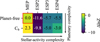 |
Fig. 2 Bayesian-evidence comparison between different planetary configurations and stellar-activity kernels. Planetary configurations include a circular-orbit component (Cb; e = 0). For stellar activity, we utilised the MEP kernel and the ESP kernel with two, three, and four harmonics. The model that we elected for analysis assumed a planet-free model with a MEP kernel (red border; ln Z = -434.4). We give the Bayesian factor Δ ln Z of remaining models relative to this model. |
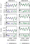 |
Fig. 3 Raw time series (markers) against our best model (black; LTF+GP) in two selected intervals. The data points come with two error bars: one assigned by the instrument (saturated) and another that includes the model jitter (semi-transparent). We provide a direct comparison and the associated O-C diagrams in (a,b,c,d) RV, (e,f,g,h) FWHM, and (i,j,k,l) S-index. |
5.3.1 ESPRESSO measurements
We tested whether the ESPRESSO data alone are sufficient to characterise the overall stellar activity. Figure B.4 displays the prediction of our best model that was re-run only on ESPRESSO data. No significant signals remain in the residuals except two FWHM signatures at 1.4d, 1.8d, and 3.4d (Fig. B.4d). These three signals were assigned a false-alarm probability (FAP; Baluev 2008) smaller than 1%.
We provide the posterior of this variant of the best model in Table B.1 in the column ‘ESPRESSO’. We observed only two appreciable differences between the ESPRESSO-only and the full-data best model. Firstly, the LTF cycle was not well constrained in the ESPRESSO-only model, with a Pcvc = 1720 d and a posterior shape that was sharply cut off by the prior 𝒰(1000,2000) d. This is likely because the 1500 d baseline of ESPRESSO data falls short of the inferred cycle period (1670
 d). The remaining LTF parameters deteriorated likewise. Secondly, the ESPRESSO-only model inferred a larger sinescale of η = 0.94
 (against 0.53
 ; Table B.1), which is, nevertheless, a 1σ agreement. We conclude that the inference on just these 65 ESPRESSO measurements returns very similar results to our all-data fits, except when it comes to LTF parameters. This affirms the central role of ESPRESSO data in the analysis.
5.3.2 CARMENES measurements
We tried to add CARMENES RV and FWHM measurements to our composite dataset, and to run the model grid anew. We found two apparent differences between CARMENES and the rest of the data: larger RV and FWHM scatter compared to other time series, and strong unexplained signals in both RV and FWHM (Fig. B.5). Despite having the largest median FWHM uncertainties (2.01 m s−1) and the second-largest median RV uncertainties (1.51 m s−1), the inclusion of CARMENES data in either dimension (or both) gave noticeably smaller timescales, and in most cases the posteriors converged to the lower end of the 𝒰log (20,104) d prior. Inferring our best model on the CARMENES data alone was affected by similar problems, and in this instance even the stellar-rotation period was not identified in its wide 𝒰(40.1,64.1) d prior (Fig. B.6). We attempted to preprocess CARMENES data in the different ways before inference, including (i) iterative 3σ clipping in RV and FWHM, (ii) nightly binning measurements, (iii) RVs with or without nightly zeropoint corrections (Ribas et al. 2023), and (iv) manual derivation of CCF FWHMs. None of this helped to solve the issue at hand, and this led to the exclusion of the CARMENES data from our analysis.
6 Discussion
6.1 Stellar activity of GJ 526
The stellar activity of GJ 526 in FWHM and S-index demonstrates a strong positive correlation (R = 0.85; Pearson 1895), which is apparent in Fig. 1. As such, FWHM and S-index fit nicely within the FF′ formalism, where they are modelled with the same kernel estimation G(ti,j), but under different scaling. Through our best model, we report a timescale of τ = 277 d and a stellar-rotation period of Prot = 48.7 ± 0.3 d. This implies the ratio τ/Prot = 5.7
 d, which hints towards a light-curve morphology that is not Sun-like (i.e.
  ; Giles et al. 2017). However, although disfavoured by the evidence, ESP models inferred very different timescales that suggest a Sunlike morphology; we report τ/Prot values of 1.4 ± 0.4 for ESP2, 1.6
 for ESP3, and 1.6 ± 0.4 for ESP4.
We report a sinescale of η = 0.53 , and this measurement appears stable for all planet-free models. We observe positive A0, B0, A1, A2 for all models. This hints that stellar-activity modulations correlate positively between RV and activity indicators, and between RV and the derivatives of the latter. Furthermore, A0 ≪ B0, meaning that stellar activity is more prominent in the RV gradient. These results can be interpreted in the following way. FWHM correlates positively with S-index, meaning that the former becomes wider when there are more active regions facing the observer. On the other hand, FWHM correlates negatively with stellar flux (Suárez Mascareño et al. 2020). This suggests that the active regions themselves are dark spots on the stellar surface. The positiveness of B0 implies that the RV gradient is also correlated positively with FWHM (and S-index), which would also explain this activity as a dark-spot flux effect.
We detect a weak cycle of period 1680 d with the following semi-amplitudes: 0.51
 m s−1 in RV, 2.73
 m s−1 in FWHM, and 0.019
 in S-index. Our cycle-phase uncertainties make it difficult to determine whether cycle components are in or out of phase. We report the following absolute phase differences: 0.65
 between RV and FWHM,
  between RV and S-index, and 0.08
 between FWHM and S-index. What we measure for Pcyc is approximately half that measured by Suárez Mascareño et al. (2016) (9.9 ± 2.8 yr), based on 281 photometric measurements over 6.5 yr. Recently, Ibañez Bustos et al. (2025) measured a similar value (3739 ± 288 d) from 47 S-index measurements over 12 yr. Our FWHM (N = 91) and S-index data (N = 147) over almost 26 yr show preference towards a shorter cycle, both at the GLSP stage (Fig. 1) as well as during our one-dimensional LTF selection (Sect. 5.2). Desaturated and de-mooned ASAS-SN photometry reveals a 1333 d signature that agrees with our measurement of Pcyc (Sect. A.1).
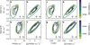 |
Fig. 4 Phase-space trajectories built from our best-model predictions in Fig. 3, in the same selected intervals. We compare RV with (a, b) FWHM, (c, d) the time derivative of FWHM, (e, f) S-index, and (g, h) the time derivative of S-index. Time runs from blue to yellow, as defined by the colour bars on the right-hand side. The same colour bars contain the temporal location of ESPRESSO18 (circles) and ESPRESSO19 (squares) measurements. Every trajectory comes with a mark at the bottom right that guides the direction of evolution, as well as the median model uncertainty in each dimension. |
6.2 Phase-space trajectories in RV, FWHM, and S-index
The two highlighted intervals in Fig. 3: intervals A and B, are among the most densely measured in our dataset. Each spans 240 d (i.e. about 5Prot) and they are also 715 d apart (i.e. about 0.4Pcyc). The dense ESPRESSO sampling allows us to peek into the stellar activity within a few stellar-rotation periods; the large gap between intervals offers the opportunity to compare them head-to-head and to look for long-term changes. We took our best-model predictions from Fig. 3, and computed the time derivatives of activity indicators, again at 0.1 d sampling10. Then, we plotted the predicted RVs against both indicators and their time derivatives, as a function of time, in Fig. 4. For instance, Fig. 4a takes the predicted RV against time (Fig. 3a) as well as the predicted FWHM against time (Fig. 3e), and plots them against one another, with time being colour-coded. These plots visualise the phase spaces between RV and activity indicators (or the time derivatives of the latter), and reveal the phase-space trajectories that GJ 526 follows over time.
Figure 4 shows phase-space trajectories over approximately 5Prot. At the same time, all trajectories comprise five closed contours that repeat themselves to some degree. This means that for each geometrical revolution of GJ 526 around itself (one Prot), we have one revolution in phase space (one contour). In addition, the trajectories reveal intricate features in stellar activity, which we now briefly address. By virtue of the apparent (and model-assumed) positive correlation between FWHM and S-index, we restrict ourselves to a discussion between RV, FWHM, and the time derivative of FWHM.
The first phase-space trajectory (Fig. 4a; RV and FWHM in Interval A) already reveals interesting features of the stellar activity of GJ 526. Here, the trajectory revolves clockwise, but the contours do not maintain the same size. The trajectory starts out small (Fig. 4a; dark-blue contour), then unwinds to a contour of a phase-space area that is several times larger at around 2 458 620-2 458 660 BJD, and then winds inwards again at the end of the interval. This behaviour can be verified by inspection of the peak-to-peak distance evolution in Fig. 3a and Fig. 3e, but it only becomes clear in a phase-space trajectory plot. It is worth mentioning that not all contours are convex; the first three contours all have an inward curl (Fig. 4a, near the origin). This is a manifestation of the flip-flop effect, i.e. a cyclic shift of active regions to the other parts of the stellar surface (Berdyugina et al. 1999; see also Oláh et al. 2006; Hackman et al. 2013), which can be again verified in the RV and FWHM time series (Figs. 3a,e).
In Interval B, almost half a cycle later, the RV-FWHM trajectory continues to revolve clockwise (Fig. 4e). We catch a remnant of a flip-flop effect at the very beginning of the interval, as well as a second curl near 2 459 270 BJD. Here, the whole phasespace trajectory is translated upwards and rightwards relative to Interval A. This suggests a positive shift in RV and FWHM, which we attribute to the long-term cycle itself. In this interval, we do not observe any apparent growth or shrinkage between contours, and their apparent centres seem to move at a slower rate than in Interval A.
We observe similar trajectory structures in the phase space formed by RV and the first FWHM derivative (Figs. 4b,f). Here, the contours are less circular, and have a more positive covariance. The trajectories revolve anticlockwise, opposite to the RV-FWHM trajectories. Curls can again be sighted, but this time they are easily spotted only in Interval A (Fig. 4b). In the same interval, we observe a similar situation of unwinding to a larger contour around 2 458 620-2 458 660 BJD, which winds inwards again at the end of the interval. This is consistent with Fig. 4a, since a large variance in the FWHM derivative would imply a large variance in FWHM as well. Finally, the apparent centre of contours only shifts upwards from Interval A to Interval B. This suggests that while FWHM appears to be offset significantly within a cycle (Figs. 4a, e), the derivative does not.
The phase-space trajectories of GJ 526 are a natural argument against the use of a direct correlation analysis between RV and activity indicators. Depending on the temporal sampling of an observing campaign, measurements may ‘land’ on different parts of the trajectory, meaning that an observer may get a positive or a negative correlation, or no correlation at all. The need to factor in the times of measurement as well as the measurements themselves has been noted in earlier works (e.g. Collier Cameron et al. 2019). Phase-space trajectories satisfy this need, and may open new doors for analysis.
We report the following median model uncertainties in Fig. 4 in RV, FWHM, FWHM derivative, S-index, and Sindex derivative: 0.74ms−1, 1.38 ms−1, 0.27 ms−1 d−1, 0.0202, and 0.0039 d−1 in Interval A; as well as 0.76 ms−1, 1.45 ms−1, 0.26ms−1d−1, 0.0212, and 0.0039d−1 in Interval B (marked with error bars in the subplots). Although these median uncertainties are larger than the intricate curls we observe in the phase spaces, we note that most curls are significant compared to their local uncertainties (e.g. near 2458 550BJD, 2458 640 BJD, and 2 459 270 BJD; Figs. 3a, b). We anticipate that the precision of a phase-space trajectory at a given time t grows with the number of measurements within one timescale τ from t, as well as with the precision of measurements themselves. As such, trajectory analyses should be conducted in well-measured intervals, even if only in one physical quantity, provided that the GP hyperparameters are sufficiently well defined.
We used the same model to analyse data from several instruments, and these data may in principle come with their own chromatic effects. In our case, however, the wavelength ranges are similar enough so that no significant chromaticity is expected for an early M dwarf (380-788 nm for ESPRESSO, 380-690nm for HARPS, 300-630 nm for HIRES RVs). There is only one time series overlap - that of HIRES and HARPS in RV and S-index - and we do not observe a strong discrepancy in behaviour or scatter in either case (Figs. 1a,e). The FWHM may have a different mean value depending on the instrumental profile, but relative variations have been shown to behave consistently while following astronomical phenomena. This consistency has been recently demonstrated between ESPRESSO and HARPS, in both RV and FWHM (Suárez Mascareño et al. 2025, Fig. F.1; Hobson et al. 2025, Fig. 6). The S-index is defined as a flux ratio of regions with strict wavelength boundaries (Eq. (1)), and is consequently expected to be invariant.
6.3 Detection limits for additional companions
Works related to exoplanetary searches often attempt to assess their sensitivity to any undiscovered planets in a system. This gives rise to different tests that probe the ‘detection limit’ of a certain study. However, the very design of these tests changes the meaning of a detection limit. For example, one way to assess sensitivity is to inject a random circular-planet signal in the raw RV data, and then to fit the best model again onto the modified raw time series, using the median posterior that had already been inferred in the main analysis. The best model may absorb the injected signal, or may leave it out, causing a strong peak in the residual GLSP in the second case. One can therefore inject different sines, one at a time, and determine sensitivity from some aggregate statistics of the injected signal after fitting (e.g. Konacki et al. 2009; Howard & Fulton 2016). Such tests are referred to as injection-recovery tests, and their detection limits are fundamentally based on the inability of their models to leave an injected RV signal out.
Other tests look for an extra planet directly in the data, with no injection or recovery. For example, Faria et al. (2020) used the sampled posteriors of their models with planets, and propagated them into a period-mass distribution. We used a variant of this test. We started with our best model, augmented it to include an extra circular-planet signal, and sampled for its parameters, having fixed all other model parameters except the RV zero offset α0 and the RV jitters Ji,011. We did this for many bins of the orbital-period space, with a separate inference run per bin. Then, for each bin, we considered the ±3σ percentiles of the RV semiamplitude posterior of the extra planet. The +3σ percentile can be interpreted as the maximum semi-amplitude an undiscovered planet would have with a 3σ probability, if it existed at all, and we took this value as our detection limit. The −3σ percentile tells of any significant signals that stand well away from the zero and that could deserve attention in further studies.
We took the orbital-period interval 𝒰log(1,1000) d, and partitioned it in 100 bins. In each of these simpler ‘bin models’, we used an RV semi-amplitude of 𝒰(0,5) ms−1, the same RV-offset prior as in our model grid, and a reduced RV-jitter prior of 𝒰(0,5) ms−1 for all instruments. To speed up the inference, in every instance of Nparam bin-model parameters, we required 20Nparam live points (instead of 40Nparam in the model grid), and integrated until 10% of the log-likelihood integral was left in the iterative remainder (instead of the default 1% in ULTRAN - EST). Figure 5 displays the ±3σ percentiles of our 100 bins in the parameter space. Overall, our +3σ detection limit stands around 1 m s−1, consistent with our model jitters (0.88-2.26 m s−1). This limit shows a very modest degradation to 1.5 ms−1 at periods in the range 20-80 d, on the same scale as Prot. The data at hand are already sensitive to the detection of any Neptune-mass planets up to 103 d, as they induce larger semi-amplitudes than the 3σ detection limit. On the other hand, the −3σ percentile never exceeds 10cms−1.
Our detection-limit test takes place in the space formed by the RV semi-amplitude and the orbital period. We took the derived stellar parameters and their uncertainties in Table 1, and used them to transform the semi-amplitude to minimum mass, as well as the orbital period to the semi-major axis (SMA). Under such transformations, we can reject the presence of planets up to a certain mass for a given SMA. Our test disfavours the presence of planets beyond 5 M⊙ in the interval 0.02-0.16 AU, and beyond 8 M⊙ in the interval 0.16-1.4 AU. At the same time, the vicinity of GJ 526 to the Sun allows the proper-motion anomaly technique to place similar limits on longer-period planets; Kervella et al. (2022) found that there appear to be no planets beyond 25-30 M⊙ in the interval 3-10 AU. Such combinations of techniques allow to screen for planets over wide ranges of orbital separations.
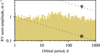 |
Fig. 5 Detection limits of GJ 526. Shaded bands show the 3σ RV semi-amplitude posterior of a modelled planet in our best model, in 100 log-spaced orbital-period bins. The two dotted lines show the RV semiamplitudes that an Earth-mass planet and a Neptune-mass planet would inject in the system. |
6.4 False-inclusion probability tests
We assessed the significance of any RV signals that escaped our modelling following Hara et al. (2022), hereafter H22. Their formalism uses the posterior distribution of an inference run to compute the probability of having no planets within a given element in the orbital-frequency space. H22 refers to this metric as the false-inclusion probability (FIP). We took the posteriors of our MEP model with one circular-orbit planet (Fig. 2; bottom left) and invoked the FIP formalism between 1-1000 d for an angular-frequency step Δω = 2π/5Tb1, where Tb1 is our dataset baseline. We found several inconspicuous peaks in the range 10100 d; the most significant was assigned a FIP of about 70% at a period near Prot. No signals passed the 1% threshold that supports a planetary detection suggested by H22.
7 Conclusions
We performed a stellar-activity analysis of GJ 526 in three physical quantities (RV, FWHM, S-index) on the rich and multi-faceted velocimetry provided by the HIRES, HARPS, and ESPRESSO instruments. Through simultaneously fitting a multi-dimensional GP model in all three quantities, we constrained the stellar-rotation period of GJ 526 to Prot = 48.7 ± 0.3 d and deduced that its active regions are dark spots on the stellar surface. We demonstrated that 65 ESPRESSO measurements alone replicate these results with an acceptable precision. The combined HIRES, HARPS, and ESPRESSO spectroscopy suggests that GJ 526 exhibits weak magnetic activity with a period of Pcyc = 1680 d. The current evidence does not support the existence of a planetary companion around GJ 526. We estimate that if such companion existed, it would likely have an RV semi-amplitude smaller than 1.5 m s−1.
We propose the use of phase-space trajectories as a way to illustrate and understand stellar activity (Sect. 6.2). We argue that their use allows the identification of less apparent details in activity. Unlike correlations between RV and activity indicators, phase-space trajectories contain temporal information and can be informative as long as the region of interest contains enough points to guarantee a precise model prediction. As an example, we qualitatively compared phase-space trajectories in RV, FWHM, and S-index in two intervals separated by almost half a magnetic cycle. Further work is required to determine the usefulness of such phase-space trajectories. For instance, it may be the case that the direction of revolution, or the geometrical features of phase-space trajectories (e.g. angular velocity or area) carry some physical meaning. These prospects can be explored through a trajectory comparison with observational data of other cool dwarfs or with synthetic data from stellar-activity simulation suites.
Acknowledgements
AKS acknowledges the support of a fellowship from the “la Caixa” Foundation (ID 100010434). The fellowship code is LCF/BQ/DI23/11990071. AKS, JIGH, ASM, NN and RR acknowledge financial support from the Spanish Ministry of Science and Innovation (MICINN) project PID2020-117493GB-I00 and from the Government of the Canary Islands project ProID2020010129. NN acknowledges funding from Light Bridges for the Doctoral Thesis “Habitable Earth-like planets with ESPRESSO and NIRPS”, in cooperation with the Instituto de Astrofísica de Canarias, and the use of Indefeasible Computer Rights (ICR) be- ing commissioned at the ASTRO POC project in the Island of Tenerife, Canary Islands (Spain). The ICR-ASTRONOMY used for his research was provided by Light Bridges in cooperation with Hewlett Packard Enterprise (HPE). Co-funded by the European Union (ERC, FIERCE, 101052347). Views and opinions expressed are however those of the author(s) only and do not necessarily reflect those of the European Union or the European Research Council. Neither the European Union nor the granting authority can be held responsible for them. This work was supported by FCT -Fundaçâo para a Ciência e a Tecnologia through national funds by these grants: UIDB/04434/2020 DOI: 10.54499/UIDB/04434/2020, UIDP/04434/2020 DOI: 10.54499/UIDP/04434/2020, PTDC/FIS-AST/4862/2020, UID/04434/2025, 2022.04048.PTDC DOI: 10.54499/2022.04048.PTDC. CJAPM also acknowledges FCT and POCH/FSE (EC) support through Investigador FCT Contract 2021.01214.CEECIND/CP1658/CT0001 (DOI 10.54499/2021.01214.CEECIND/CP1658/CT0001). AC-G is funded by the Spanish Ministry of Science through MCIN/AEI/10.13039/501100011033 grant PID2O19-107061GB-C61. This work includes data collected by the TESS mission and made use of LIGHTKURVE, a Python package for Kepler and TESS data analysis (Lightkurve Collaboration et al. 2018). Funding for the TESS mission is provided by the NASA’s Science Mission Directorate. This research has made use of NASA’s Astrophysics Data System Bibliographic Services. We made use of NASA’s Astrophysics Data System, which is operated by the California Institute of Technology, under contract with the National Aeronautics and Space Administration under the Exoplanet Exploration Program. This research has made use of the SIMBAD (Wenger et al. 2000) and VIZIER (Ochsenbein et al. 2000) databases, both operated at CDS, Strasbourg, France. Additionally, we made use of the Revised Version of the New Catalogue of Suspected Variable Stars (Kazarovets et al. 2022). We thank the anonymous referee for their time and effort. AKS acknowledges Jean-Baptiste Delisle for the prompt support on some technical queries regarding S+LEAF. We used the following PYTHON packages for data analysis and visualisation: ASTROPY (Astropy Collaboration 2022), MATPLOTLIB (Hunter 2007), NIEVA (Stefanov et al., in prep.), NUMPY (Harris et al. 2020), PANDAS (McKinney 2010; The Pandas Development Team 2022), SCIPY (Virtanen et al. 2020), SEABORN (Waskom 2021), S+LEAF (Delisle et al. 2020, 2022) and ULTRANEST (Buchner 2021). This manuscript was written and compiled in OVERLEAF. All presented analysis was conducted on UBUNTU machines. The bulk of modelling and inference was done on the Diva cluster (192 Xeon E7-4850 2.1GHz CPUs; 4.4 TB RAM) at Instituto de Astrofísica de Canarias, Tenerife, Spain.
References
- Ahrer, E., Queloz, D., Rajpaul, V. M., et al. 2021, MNRAS, 503, 1248 [NASA ADS] [CrossRef] [Google Scholar]
- Aigrain, S., Pont, F., & Zucker, S. 2012, MNRAS, 419, 3147 [NASA ADS] [CrossRef] [Google Scholar]
- Allard, F., Homeier, D., & Freytag, B. 2012, Philos. Trans. Roy. Soc. A: Math. Phys. Eng. Sci., 370, 2765 [Google Scholar]
- Angus, R., Morton, T., Aigrain, S., Foreman-Mackey, D., & Rajpaul, V. 2018, MNRAS, 474, 2094 [Google Scholar]
- Antoniadis-Karnavas, A., Sousa, S. G., Delgado-Mena, E., Santos, N. C., & Andreasen, D. T. 2024, A&A, 690, A58 [NASA ADS] [CrossRef] [EDP Sciences] [Google Scholar]
- Astropy Collaboration (Price-Whelan, A. M., et al.) 2022, ApJ, 935, 167 [NASA ADS] [CrossRef] [Google Scholar]
- Baluev, R. V. 2008, MNRAS, 385, 1279 [Google Scholar]
- Baranne, A., Queloz, D., Mayor, M., et al. 1996, A&AS, 119, 373 [NASA ADS] [CrossRef] [EDP Sciences] [Google Scholar]
- Barragán, O., Gillen, E., Aigrain, S., et al. 2023, MNRAS, 522, 3458 [CrossRef] [Google Scholar]
- Bayo, A., Rodrigo, C., Barrado Y Navascués, D., et al. 2008, A&A, 492, 277 [NASA ADS] [CrossRef] [EDP Sciences] [Google Scholar]
- Beichman, C. A., Neugebauer, G., Habing, H. J., Clegg, P. E., & Chester, T. J. 1988, Infrared Astronomical Satellite (IRAS) Catalogs and Atlases. Volume 1: Explanatory Supplement, 1 [Google Scholar]
- Berdyugina, S. V., Berdyugin, A. V., Ilyin, I., & Tuominen, I. 1999, A&A, 350, 626 [Google Scholar]
- Bianchi, L., Shiao, B., & Thilker, D. 2017, ApJS, 230, 24 [Google Scholar]
- Binks, A. S., & Jeffries, R. D. 2016, MNRAS, 455, 3345 [Google Scholar]
- Borgniet, S., Meunier, N., & Lagrange, A. M. 2015, A&A, 581, A133 [NASA ADS] [CrossRef] [EDP Sciences] [Google Scholar]
- Buchner, J. 2021, J. Open Source Softw., 6, 3001 [CrossRef] [Google Scholar]
- Butler, R. P., Marcy, G. W., Williams, E., Hauser, H., & Shirts, P. 1997, ApJ, 474, L115 [Google Scholar]
- Butler, R. P., Marcy, G. W., Fischer, D. A., et al. 1999, ApJ, 526, 916 [NASA ADS] [CrossRef] [Google Scholar]
- Butler, R. P., Vogt, S. S., Laughlin, G., et al. 2017, AJ, 153, 208 [Google Scholar]
- Caldwell, D. A., Tenenbaum, P., Twicken, J. D., et al. 2020, RNAAS, 4, 201 [NASA ADS] [Google Scholar]
- Castro-González, A., Demangeon, O. D. S., Lillo-Box, J., et al. 2023, A&A, 675, A52 [NASA ADS] [CrossRef] [EDP Sciences] [Google Scholar]
- Chambers, K. C., Magnier, E. A., Metcalfe, N., et al. 2016, The Pan-STARRS1 Surveys [Google Scholar]
- Collier Cameron, A., Mortier, A., Phillips, D., et al. 2019, MNRAS, 487, 1082 [Google Scholar]
- Cutri, R. M., Skrutskie, M. F., van Dyk, S., et al. 2003, VizieR Online Data Catalog, II/246 [Google Scholar]
- Damasso, M., Rodrigues, J., Castro-González, A., et al. 2023, A&A, 679, A33 [NASA ADS] [CrossRef] [EDP Sciences] [Google Scholar]
- Dawson, R. I., & Fabrycky, D. C. 2010, ApJ, 722, 937 [Google Scholar]
- de Lalande, J. J. L. F. 1801, Histoire Celeste Francaise, Contenant Les Observations Faites Par Plusieurs Astronomes Francais [Google Scholar]
- Delisle, J. B., Hara, N., & Ségransan, D. 2020, A&A, 638, A95 [EDP Sciences] [Google Scholar]
- Delisle, J.-B., Unger, N., Hara, N. C., & Ségransan, D. 2022, A&A, 659, A182 [NASA ADS] [CrossRef] [EDP Sciences] [Google Scholar]
- Dumusque, X., Lovis, C., Ségransan, D., et al. 2011, A&A, 535, A55 [NASA ADS] [CrossRef] [EDP Sciences] [Google Scholar]
- Faria, J. P., Adibekyan, V., Amazo-Gómez, E. M., et al. 2020, A&A, 635, A13 [NASA ADS] [CrossRef] [EDP Sciences] [Google Scholar]
- Faria, J. P., Suárez Mascareño, A., Figueira, P., et al. 2022, A&A, 658, A115 [NASA ADS] [CrossRef] [EDP Sciences] [Google Scholar]
- Fetherolf, T., Pepper, J., Simpson, E., et al. 2023, ApJS, 268, 4 [NASA ADS] [CrossRef] [Google Scholar]
- Fischer, D. A., Marcy, G. W., & Spronck, J. F. P. 2014, ApJS, 210, 5 [Google Scholar]
- Fuhrmeister, B., Czesla, S., Schmitt, J. H. M. M., et al. 2019, A&A, 623, A24 [NASA ADS] [CrossRef] [EDP Sciences] [Google Scholar]
- Gaia Collaboration (Vallenari, A., et al.) 2022, Gaia Data Release 3: Summary of the Content and Survey Properties [Google Scholar]
- Gaidos, E., Mann, A. W., Lépine, S., et al. 2014, MNRAS, 443, 2561 [Google Scholar]
- Giles, H. A. C., Collier Cameron, A., & Haywood, R. D. 2017, MNRAS, 472, 1618 [Google Scholar]
- González Hernández, J. I., Suárez Mascareño, A., Silva, A. M., et al. 2024, A&A, 690, A79 [NASA ADS] [CrossRef] [EDP Sciences] [Google Scholar]
- Hackman, T., Pelt, J., Mantere, M. J., et al. 2013, A&A, 553, A40 [NASA ADS] [CrossRef] [EDP Sciences] [Google Scholar]
- Hara, N. C., Unger, N., Delisle, J.-B., Díaz, R. F., & Ségransan, D. 2022, A&A, 663, A14 [NASA ADS] [CrossRef] [EDP Sciences] [Google Scholar]
- Harris, C. R., Millman, K. J., van der Walt, S. J., et al. 2020, Nature, 585, 357 [NASA ADS] [CrossRef] [Google Scholar]
- Haywood, R. D. 2015, PhD thesis [Google Scholar]
- Haywood, R. D., Collier Cameron, A., Queloz, D., et al. 2014, MNRAS, 443, 2517 [Google Scholar]
- Hobson, M., Suárez Mascareño, A., Lovis, C., et al. 2025, A&A, 702, A32 [NASA ADS] [CrossRef] [EDP Sciences] [Google Scholar]
- Høg, E., Fabricius, C., Makarov, V. V., et al. 2000, A&A, 355, L27 [Google Scholar]
- Howard, A. W., & Fulton, B. J. 2016, PASP, 128, 114401 [NASA ADS] [CrossRef] [Google Scholar]
- Huang, C. X., Vanderburg, A., Pál, A., et al. 2020a, RNAAS, 4, 204 [Google Scholar]
- Huang, C. X., Vanderburg, A., Pál, A., et al. 2020b, RNAAS, 4, 206 [Google Scholar]
- Hunter, J. D. 2007, Comput. Sci. Eng., 9, 90 [NASA ADS] [CrossRef] [Google Scholar]
- Ibañez Bustos, R. V., Buccino, A. P., Nardetto, N., et al. 2025, A&A, 696, A230 [NASA ADS] [CrossRef] [EDP Sciences] [Google Scholar]
- Ishihara, D., Onaka, T., Kataza, H., et al. 2010, A&A, 514, A1 [NASA ADS] [CrossRef] [EDP Sciences] [Google Scholar]
- Jenkins, J. M., Twicken, J. D., McCauliff, S., et al. 2016, SPIE Proc., 9913, 99133E [Google Scholar]
- Kazarovets, E. V., Samus, N. N., & Durlevich, O. V. 2022, Astron. Rep., 66, 555 [NASA ADS] [CrossRef] [Google Scholar]
- Kervella, P., Arenou, F., & Thévenin, F. 2022, A&A, 657, A7 [NASA ADS] [CrossRef] [EDP Sciences] [Google Scholar]
- Kochanek, C. S., Shappee, B. J., Stanek, K. Z., et al. 2017, PASP, 129, 104502 [Google Scholar]
- Konacki, M., Muterspaugh, M. W., Kulkarni, S. R., & Helminiak, K. G. 2009, ApJ, 704, 513 [Google Scholar]
- Kunimoto, M., Huang, C., Tey, E., et al. 2021, RNAAS, 5, 234 [NASA ADS] [Google Scholar]
- Kunimoto, M., Tey, E., Fong, W., et al. 2022, RNAAS, 6, 236 [NASA ADS] [Google Scholar]
- Levenberg, K. 1944, Quart. Appl. Math., 2, 164 [Google Scholar]
- Lightkurve Collaboration, Cardoso, J. V. d. M., Hedges, C., et al. 2018, Astrophysics Source Code Library [ascl:1812.013] [Google Scholar]
- Lomb, N. R. 1976, Ap&SS, 39, 447 [Google Scholar]
- Lovis, C., Mayor, M., Bouchy, F., et al. 2005, A&A, 437, 1121 [NASA ADS] [CrossRef] [EDP Sciences] [Google Scholar]
- Mann, A. W., Dupuy, T., Kraus, A. L., et al. 2019, ApJ, 871, 63 [Google Scholar]
- Marcy, G. W., & Butler, R. P. 1996, ApJ, 464, L147 [NASA ADS] [CrossRef] [Google Scholar]
- Marfil, E., Tabernero, H. M., Montes, D., et al. 2021, A&A, 656, A162 [NASA ADS] [CrossRef] [EDP Sciences] [Google Scholar]
- Marquardt, D. W. 1963, J. Soc. Ind. Appl. Math., 11, 431 [Google Scholar]
- Martinez, A. O., Crossfield, I. J. M., Schlieder, J. E., et al. 2017, ApJ, 837, 72 [Google Scholar]
- Mayor, M., Pepe, F., Queloz, D., et al. 2003, The Messenger, 114, 20 [NASA ADS] [Google Scholar]
- McKinney, W. 2010, in Python in Science Conference (Austin, Texas), 56 [Google Scholar]
- Noyes, R. W., Hartmann, L. W., Baliunas, S. L., Duncan, D. K., & Vaughan, A. H. 1984, ApJ, 279, 763 [Google Scholar]
- Ochsenbein, F., Bauer, P., & Marcout, J. 2000, A&AS, 143, 23 [NASA ADS] [CrossRef] [EDP Sciences] [Google Scholar]
- Oláh, K., Korhonen, H., Kővári, Zs., Forgács-Dajka, E., & Strassmeier, K. G. 2006, A&A, 452, 303 [NASA ADS] [CrossRef] [EDP Sciences] [Google Scholar]
- Pancino, E., Lardo, C., Altavilla, G., et al. 2017, A&A, 598, A5 [NASA ADS] [CrossRef] [EDP Sciences] [Google Scholar]
- Passegger, V. M., Bello-García, A., Ordieres-Meré, J., et al. 2022, A&A, 658, A194 [NASA ADS] [CrossRef] [EDP Sciences] [Google Scholar]
- Passegger, V. M., Suárez Mascareño, A., Allart, R., et al. 2024, A&A, 684, A22 [NASA ADS] [CrossRef] [EDP Sciences] [Google Scholar]
- Pearson, K. 1895, Proc. Roy. Soc. Lond. Ser. I, 58, 240 [NASA ADS] [CrossRef] [Google Scholar]
- Pepe, F., Molaro, P., Cristiani, S., et al. 2014, Astron. Nachr., 335, 8 [Google Scholar]
- Pepe, F., Cristiani, S., Rebolo, R., et al. 2021, A&A, 645, A96 [NASA ADS] [CrossRef] [EDP Sciences] [Google Scholar]
- Pinamonti, M., Damasso, M., Marzari, F., et al. 2018, A&A, 617, A104 [NASA ADS] [CrossRef] [EDP Sciences] [Google Scholar]
- Pojmanski, G. 1997, Acta Astron., 47, 467 [Google Scholar]
- Porter, J. G. 1892, AJ, 12, 25 [Google Scholar]
- Quirrenbach, A., Amado, P. J., Caballero, J. A., et al. 2014, SPIE Conf. Proc., 9147, 91471F [Google Scholar]
- Quirrenbach, A., Amado, P. J., Caballero, J. A., et al. 2016, SPIE Conf. Proc., 9908, 990812 [Google Scholar]
- Rajpaul, V., Aigrain, S., Osborne, M. A., Reece, S., & Roberts, S. 2015, MNRAS, 452, 2269 [Google Scholar]
- Rajpaul, V. M., Buchhave, L. A., Lacedelli, G., et al. 2021, MNRAS, 507, 1847 [NASA ADS] [CrossRef] [Google Scholar]
- Rasmussen, C. E., & Williams, C. K. I. 2006, Gaussian Processes for Machine Learning, Adaptive Computation and Machine Learning (Cambridge, Mass: MIT Press) [Google Scholar]
- Ribas, I., Reiners, A., Zechmeister, M., et al. 2023, A&A, 670, A139 [NASA ADS] [CrossRef] [EDP Sciences] [Google Scholar]
- Ricker, G. R., Winn, J. N., Vanderspek, R., et al. 2015, J. Astron. Telesc. Instrum. Syst., 1, 014003 [Google Scholar]
- Rojas-Ayala, B., Covey, K. R., Muirhead, P. S., & Lloyd, J. P. 2012, ApJ, 748, 93 [Google Scholar]
- Scargle, J. D. 1982, ApJ, 263, 835 [Google Scholar]
- Schweitzer, A., Passegger, V. M., Cifuentes, C., et al. 2019, A&A, 625, A68 [NASA ADS] [CrossRef] [EDP Sciences] [Google Scholar]
- Shakhovskaya, N. I. 1971, Veröff. Remeis-Sternwarte Bamberg, 9, 138 [Google Scholar]
- Shappee, B. J., Prieto, J. L., Grupe, D., et al. 2014, ApJ, 788, 48 [Google Scholar]
- Silva, A. M., Faria, J. P., Santos, N. C., et al. 2022, A&A, 663, A143 [NASA ADS] [CrossRef] [EDP Sciences] [Google Scholar]
- Skilling, J. 2004, AIP Conf. Proc., 735, 395 [Google Scholar]
- Sousa, S. G., Adibekyan, V., Delgado-Mena, E., et al. 2021, A&A, 656, A53 [NASA ADS] [CrossRef] [EDP Sciences] [Google Scholar]
- Stefanov, A. K., Suárez Mascareño, A., González Hernández, J. I., et al. 2025, A&A, 695, A62 [NASA ADS] [CrossRef] [EDP Sciences] [Google Scholar]
- Suárez Mascareño, A., Rebolo, R., & González Hernández, J. I. 2016, A&A, 595, A12 [Google Scholar]
- Suárez Mascareño, A., Rebolo, R., González Hernández, J. I., & Esposito, M. 2017, MNRAS, 468, 4772 [Google Scholar]
- Suárez Mascareño, A., Rebolo, R., González Hernández, J. I., et al. 2018, A&A, 612, A89 [NASA ADS] [CrossRef] [EDP Sciences] [Google Scholar]
- Suárez Mascareño, A., Faria, J. P., Figueira, P., et al. 2020, A&A, 639, A77 [Google Scholar]
- Suárez Mascareño, A., González-Álvarez, E., Zapatero Osorio, M. R., et al. 2023, A&A, 670, A5 [NASA ADS] [CrossRef] [EDP Sciences] [Google Scholar]
- Suárez Mascareño, A., Artigau, É., Mignon, L., et al. 2025, A&A, 700, A11 [NASA ADS] [CrossRef] [EDP Sciences] [Google Scholar]
- Tabernero, H. M., Marfil, E., Montes, D., & González Hernández, J. I. 2022, A&A, 657, A66 [NASA ADS] [CrossRef] [EDP Sciences] [Google Scholar]
- Tal-Or, L., Trifonov, T., Zucker, S., Mazeh, T., & Zechmeister, M. 2019, MNRAS, 484, L8 [Google Scholar]
- The Pandas Development Team. 2022, Pandas-Dev/Pandas: Pandas, Zenodo [Google Scholar]
- Trifonov, T., Tal-Or, L., Zechmeister, M., et al. 2020, A&A, 636, A74 [NASA ADS] [CrossRef] [EDP Sciences] [Google Scholar]
- Trifonov, T., Caballero, J. A., Morales, J. C., et al. 2021, Science, 371, 1038 [Google Scholar]
- van Belle, G. T., & von Braun, K. 2009, ApJ, 694, 1085 [NASA ADS] [CrossRef] [Google Scholar]
- VanderPlas, J. T., & IveziC, Z. 2015, ApJ, 812, 18 [NASA ADS] [CrossRef] [Google Scholar]
- Vaughan, A. H., Preston, G. W., & Wilson, O. C. 1978, PASP, 90, 267 [Google Scholar]
- Virtanen, P., Gommers, R., Oliphant, T. E., et al. 2020, Nat. Methods, 17, 261 [Google Scholar]
- Vogt, S. S., Allen, S. L., Bigelow, B. C., et al. 1994, in 1994 Symposium on Astronomical Telescopes & Instrumentation for the 21st Century, eds. D. L. Crawford, & E. R. Craine (Kailua, Kona, HI), 362 [Google Scholar]
- Waskom, M. 2021, J. Open Source Softw., 6, 3021 [CrossRef] [Google Scholar]
- Wenger, M., Ochsenbein, F., Egret, D., et al. 2000, A&AS, 143, 9 [NASA ADS] [CrossRef] [EDP Sciences] [Google Scholar]
- Winecki, D., & Kochanek, C. S. 2024, ApJ, 971, 61 [NASA ADS] [CrossRef] [Google Scholar]
- Wright, E. L., Eisenhardt, P. R. M., Mainzer, A. K., et al. 2010, AJ, 140, 1868 [Google Scholar]
- York, D. G., Adelman, J., Anderson, Jr., J. E., et al. 2000, AJ, 120, 1579 [NASA ADS] [CrossRef] [Google Scholar]
- Zechmeister, M., & Kürster, M. 2009, A&A, 496, 577 [CrossRef] [EDP Sciences] [Google Scholar]
Measurements came from the following programmes: 106.21M2, 108.2254, 110.24CD, 1102.C-0744, 1102.C-0958, and 1104.C-0350.
Those measurements took place near the following BJD timestamps: 2459278.8, 2459284.7, 2459289.7, 2459289.9, 2459299.7, 2459313.7, 2459322.7, and 2459327.6.
Also known as the quasi-periodic (QP) kernel in the literature.
This implies the conditions assumed in S25: (i)  , (ii) max ti,j = 0; see Sect. 3 of the same work for more details.
We computed activity-indicator time derivatives numerically through the centred finite-difference method ![Mathematical equation: $f'(x)|_{x_i}=[f(x_{i+1})-f(x_{i-1})]/2h$](/articles/aa/full_html/2025/11/aa56346-25/aa56346-25-eq299.png) , with h = 0.1 d. We used the matrix representation of this method to transform the conditional mean vector and the covariance matrix of each activity indicator so as to get to the conditional mean vector and the covariance matrix of its time derivative.
, with h = 0.1 d. We used the matrix representation of this method to transform the conditional mean vector and the covariance matrix of each activity indicator so as to get to the conditional mean vector and the covariance matrix of its time derivative.
The uneven sampling of a potential planet introduces its own RV offset, hence the need of sampling for α0. Such planets may also change the model jitters in RV, hence the need of sampling for Ji,0.
Appendix A GJ 526 photometry
Appendix A.1 ASAS-SN photometry
We used the ASAS-SN Sky Patrol online service12 to inspect the photometry of GJ 526 at hand. Our preliminary check of the field revealed that there are no significant contaminators that can bias photometry (Fig. A.1). However, the total proper motion of GJ 526 approaches 2.3″/yr (GDR3), which is comparable to the pixel size of the detector (8″). Past works address this issue through a computation of many separate light curves associated with smaller temporal intervals (e.g. Trifonov et al. 2021; Castro-González et al. 2023; Damasso et al. 2023). We went forward with the same procedure. We did split the region 2 456 000-2 461 000 JD in timestamps of 250 JD. Then, for each time stamp, we computed the expected position of GJ 526 and used the Sky Patrol service to compute an individual light curve for the temporal region defined by ±125JD around the time stamp. We used the saturated-stars photometry method as described in Winecki & Kochanek (2024). Finally, we concatenated individual light curves together, removed all points of lunar separation below 90 deg and clipped the remainder at 3σ. This procedure yielded 354 data points in Sloan g, and 99 data points in Johnson V.
Figure A.2 displays our ASAS-SN data. The rms of measurements against the median photometric uncertainty is 55 mmag against 37 mmag for Sloan g; and 41 mmag against 37 mmag for Johnson V. The observed rms can explain the variations measured by Shakhovskaya (1971) (Δmv = 40 mmag). Both time series follow an apparent trend, which manifested in the GLSPs as strong powers at infinite period. We did a linear fit on photometry (as highlighted by lines in Figs. A.3a,c), which partly, but not completely suppressed these infinite-period powers. Sloan g data appears featureless, except a large power in the range 2000-3000 d. Johnson V data, on the other hand, contains two significant peaks: one at 27.9 d and another at 1333 d. The former is close to the lunar orbital period, but we note a strong WF peak at the same location in these time series13, meaning that the 27.9 d signature in photometry likely comes from the interaction between the WF peak in question at the infinite-period power, as described in (4). After higher-order polynomial fitting, the 27.9 d peak disappeared, which confirmed our suspicions. The 1333 d peak is somewhat close to our measurements of a magnetic cycle at period Pcyc = 1670 ± 40 d.
Appendix A.2 ASAS photometry
We took all GJ 526 ASAS photometry of quality flag A or B, following Suárez Mascareño et al. (2016). Additionally, we required a minimum lunar separation of 90 deg, much like our ASAS-SN photometry. This query returned 150 data points in ASAS V with an rms of 17 mmag and a median uncertainty of 8 mmag. Photometry appears relatively stable and follows an inconspicuous linear trend with time (Fig. A.3a). After subtraction of said trend, no strong signatures remain in the GLSP (Fig. A.3b).
Appendix A.3 TESS photometry
There is available GJ 526 photometry in two TESS sectors: S23 and S50. S23 photometry was obtained in the primary mission and was analysed by the official pipeline, SPOC (Jenkins et al. 2016) - as well as by TESS-SPOC (Caldwell et al. 2020) and QLP (Huang et al. 2020a,b; Kunimoto et al. 2021, 2022) on the 30-minute FFIs. As a result, there are light-curves of 2 min and 30 min cadence in this sector alone. S50 photometry took place during the extended TESS mission, and was reduced by the QLP pipeline only, producing a light-curve of 30 min cadence. All of this amounts to four data products in total from both sectors. We present their photometry in Fig. A.4.
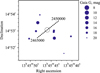 |
Fig. A.1 Proper motion of GJ 526 (black open circle) on the sky plane relative to other stars in the vicinity (blue circles). The line shows the trajectory of GJ 526 in the interval 2 450 000-2 465 000 JD, with small circular markers at every 1000 JD. The stars are size-coded relative to their brightness in Gaia G (Gaia Collaboration 2022). |
We took all aforementioned data, clipped it at 3σ and normalised it through division by the flux mean of each time series. We show the normalises time series Fig. A.4. Overall, we observe long-term trends in both S23 and S50, which are qualitatively similar and follow the same order: (i) a linear decline; (ii) a short curl upwards; (iii) a plateau until the first half of photometric coverage; (iv) a smooth rise in the second half. S23 and S50 are separated by more than 700 d, which makes any physical explanation unfavourable. Among all GLSPs, we note strong signals near 5 d, 7 d and 13 d. All of these signatures fall at periods where light-curve modulations can be attributed to instrument systematics (Fetherolf et al. 2023).
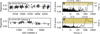 |
Fig. A.2 ASAS-SN photometry of GJ 526 discussed in this work, in: (a) Sloan g, (c) Johnson V. (b,d) The associated Lomb-Scargle periodograms of data after linear detrending. |
 |
Fig. A.3 ASAS-SN photometry of GJ 526 that we discuss in this work. (a) ASAS V time series. (b) The associated Lomb-Scargle periodogram of data after linear detrending. |
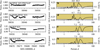 |
Fig. A.4 TESS photometry of GJ 526 discussed in this work, from the following pipelines: (a) SPOC PDCSAP from Sector 23, (c) TESS-SPOC from Sector 23, (e) QLP from Sector 23, (g) QLP from Sector 50. (b,d,f,h) The associated Lomb-Scargle periodograms of data. |
Appendix B Supplementary material
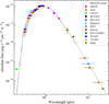 |
Fig. B.1 Observed spectral energy distribution of GJ 526 (coloured dots) from the ultraviolet through the mid-infrared. We compare those against a solar-metallicity, log g = 5.0, 3700 K PHOENIX model (grey line). |
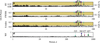 |
Fig. B.2 Alias analysis of raw time series: (a) RV, (b) FWHM, (c) S-index. We focus on the aliases of the 48.6 d signal. (d) The window function reveals four prominent peaks at 215 d (upward teal triangle), 365 d (blue circle), 475 d (downward red triangle), and 635 d (green square). The relevant aliases in data periodograms are plotted with dashed lines of a corresponding colour and marker. |
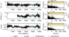 |
Fig. B.3 Raw time series (markers) against our best model (black; LTF+GP), over the whole dataset baseline in (a) RV, (c) FWHM, (e) S-index. The data points come with two error bars: one assigned by the instrument (saturated) and another that includes the model jitter (semi-transparent). (b,d,f) Associated GLSPs of the residual time series of our best model, accounting for the model jitter. |
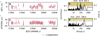 |
Fig. B.5 CARMENES 3σ clipped time series of mean-subtracted: (a) RV, (c) FWHM. (b,d) Associated wide-period GLSPs of RV and FWHM. Three FAP levels: 10%, 1% and 0.1%, split GLSP ordinates in bands of different colour. We highlight the three most prominent peaks in each GLSP. |
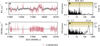 |
Fig. B.6 As in Fig. B.3, but for a derivative of the best model that was fit on CARMENES 3σ clipped data alone. |
Parameter posteriors of our best model on all data, against the same set up on ESPRESSO data alone.
All Tables
Parameter posteriors of our best model on all data, against the same set up on ESPRESSO data alone.
All Figures
|
Fig. 1 Time series of mean-subtracted (a) RV, (c) FWHM, (e) S-index. The measurements are marked according to the data source: pink downward triangles for HIRES, teal upward triangles for HARPS, blue circles for ESPRESSO18, and green squares for ESPRESSO19. (b,d,f) Associated wide-period GLSPs of RV and activity indicators. Three FAP levels: 10%, 1%, and 0.1%, split GLSP ordinates in bands of different colours. We highlight the three most prominent peaks in each GLSP. |
| In the text | |
|
Fig. 2 Bayesian-evidence comparison between different planetary configurations and stellar-activity kernels. Planetary configurations include a circular-orbit component (Cb; e = 0). For stellar activity, we utilised the MEP kernel and the ESP kernel with two, three, and four harmonics. The model that we elected for analysis assumed a planet-free model with a MEP kernel (red border; ln Z = -434.4). We give the Bayesian factor Δ ln Z of remaining models relative to this model. |
| In the text | |
|
Fig. 3 Raw time series (markers) against our best model (black; LTF+GP) in two selected intervals. The data points come with two error bars: one assigned by the instrument (saturated) and another that includes the model jitter (semi-transparent). We provide a direct comparison and the associated O-C diagrams in (a,b,c,d) RV, (e,f,g,h) FWHM, and (i,j,k,l) S-index. |
| In the text | |
|
Fig. 4 Phase-space trajectories built from our best-model predictions in Fig. 3, in the same selected intervals. We compare RV with (a, b) FWHM, (c, d) the time derivative of FWHM, (e, f) S-index, and (g, h) the time derivative of S-index. Time runs from blue to yellow, as defined by the colour bars on the right-hand side. The same colour bars contain the temporal location of ESPRESSO18 (circles) and ESPRESSO19 (squares) measurements. Every trajectory comes with a mark at the bottom right that guides the direction of evolution, as well as the median model uncertainty in each dimension. |
| In the text | |
|
Fig. 5 Detection limits of GJ 526. Shaded bands show the 3σ RV semi-amplitude posterior of a modelled planet in our best model, in 100 log-spaced orbital-period bins. The two dotted lines show the RV semiamplitudes that an Earth-mass planet and a Neptune-mass planet would inject in the system. |
| In the text | |
|
Fig. A.1 Proper motion of GJ 526 (black open circle) on the sky plane relative to other stars in the vicinity (blue circles). The line shows the trajectory of GJ 526 in the interval 2 450 000-2 465 000 JD, with small circular markers at every 1000 JD. The stars are size-coded relative to their brightness in Gaia G (Gaia Collaboration 2022). |
| In the text | |
|
Fig. A.2 ASAS-SN photometry of GJ 526 discussed in this work, in: (a) Sloan g, (c) Johnson V. (b,d) The associated Lomb-Scargle periodograms of data after linear detrending. |
| In the text | |
|
Fig. A.3 ASAS-SN photometry of GJ 526 that we discuss in this work. (a) ASAS V time series. (b) The associated Lomb-Scargle periodogram of data after linear detrending. |
| In the text | |
|
Fig. A.4 TESS photometry of GJ 526 discussed in this work, from the following pipelines: (a) SPOC PDCSAP from Sector 23, (c) TESS-SPOC from Sector 23, (e) QLP from Sector 23, (g) QLP from Sector 50. (b,d,f,h) The associated Lomb-Scargle periodograms of data. |
| In the text | |
|
Fig. B.1 Observed spectral energy distribution of GJ 526 (coloured dots) from the ultraviolet through the mid-infrared. We compare those against a solar-metallicity, log g = 5.0, 3700 K PHOENIX model (grey line). |
| In the text | |
|
Fig. B.2 Alias analysis of raw time series: (a) RV, (b) FWHM, (c) S-index. We focus on the aliases of the 48.6 d signal. (d) The window function reveals four prominent peaks at 215 d (upward teal triangle), 365 d (blue circle), 475 d (downward red triangle), and 635 d (green square). The relevant aliases in data periodograms are plotted with dashed lines of a corresponding colour and marker. |
| In the text | |
|
Fig. B.3 Raw time series (markers) against our best model (black; LTF+GP), over the whole dataset baseline in (a) RV, (c) FWHM, (e) S-index. The data points come with two error bars: one assigned by the instrument (saturated) and another that includes the model jitter (semi-transparent). (b,d,f) Associated GLSPs of the residual time series of our best model, accounting for the model jitter. |
| In the text | |
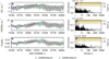 |
Fig. B.4 As in Fig. B.3, but for a derivative of the best model that was fit on ESPRESSO data alone. |
| In the text | |
|
Fig. B.5 CARMENES 3σ clipped time series of mean-subtracted: (a) RV, (c) FWHM. (b,d) Associated wide-period GLSPs of RV and FWHM. Three FAP levels: 10%, 1% and 0.1%, split GLSP ordinates in bands of different colour. We highlight the three most prominent peaks in each GLSP. |
| In the text | |
|
Fig. B.6 As in Fig. B.3, but for a derivative of the best model that was fit on CARMENES 3σ clipped data alone. |
| In the text | |
Current usage metrics show cumulative count of Article Views (full-text article views including HTML views, PDF and ePub downloads, according to the available data) and Abstracts Views on Vision4Press platform.
Data correspond to usage on the plateform after 2015. The current usage metrics is available 48-96 hours after online publication and is updated daily on week days.
Initial download of the metrics may take a while.