| Issue |
A&A
Volume 703, November 2025
|
|
|---|---|---|
| Article Number | A119 | |
| Number of page(s) | 16 | |
| Section | Stellar structure and evolution | |
| DOI | https://doi.org/10.1051/0004-6361/202556385 | |
| Published online | 20 November 2025 | |
Revisiting the extremely long-period cataclysmic variables V479 Andromedae and V1082 Sagittarii
1
Universidad Nacional Autónoma de México, Instituto de Astronomía, Aptdo Postal 6106, Ensenada, 22860 Baja California, Mexico
2
São Paulo State University (UNESP), School of Engineering and Sciences, Guaratinguetá, Brazil
3
European Southern Observatory, Karl Schwarzschild Straße 2, D-85748 Garching, Germany
4
Hamburger Sternwarte, University of Hamburg, Gojenbergsweg 112, 21029 Hamburg, Germany
5
Department of Physics and Astronomy, Texas Tech University, 2500 Broadway, Lubbock, TX 79409, USA
6
Department of Physics, University of Warwick, Coventry CV4 7AL, United Kingdom
7
American Association of Variable Star Observers (AAVSO), 185 Alewife Brook Pkwy, Suite 410, Cambridge, MA 02138, USA
8
Observadores de Supernovas (ObSN), Observatorio Cerro del Viento, MPC I84, Pl. Fernández Pirfano 3-5A, Badajoz 06010, Spain
9
Department of Astronomy, University of Washington, Seattle, WA 98195, USA
10
INAF - Osservatorio Astronomico di Capodimonte, Salita Moiariello 16, 80131 Naples, Italy
11
Departamento de Física, Universidad Técnica Federico Santa María, Av. España 1680, Valparaíso, Chile
12
Space Telescope Science Institute, 3700 San Martin Drive, Baltimore, MD 21218, USA
13
Eureka Scientific, Inc., 2452 Delmer Street Suite 100, Oakland, CA 94602-3017, USA
14
Silesian University of Technology, Akademicka 16, Gliwice, Poland
15
Observadores de Supernovas (ObSN), Observatorio Major de Dalt, C/ Major 54-2, Sant Celoni, Barcelona 08470, Spain
16
Abbey Ridge Observatory, 45 Abbey Rd, Stillwater Lake, NS B3Z1R1, Canada
17
Observadores de Supernovas (ObSN), Observatorio Magalofes, MPC Y85, C/ Feal 20, Fene, A Coruña 15509, Spain
18
Madrona Peak Observatory, 4635 Shadow Grass Dr, Katy, TX 77493, USA
19
Supra Solem Observing, SkiesAway Remote Observatory, Bradley, CA, USA
20
Observadores de Supernovas (ObSN), Observatorio El Llagarń, C/ Rio Dobra 18, Oviedo 33010, Spain
21
Vereniging voor Sterrenkunde, Zeeweg 96, 8200 Brugge, Belgium
22
Observadores de Supernovas (ObSN), Observatorio Estelia, MPC Y90, C/ Ladines 12, Ladines, Asturias 33993, Spain
23
Observadores de Supernovas (ObSN), Observatorio LaVara, MPC J38, Barrio La Vara s/n, Valdés, Asturias 33784, Spain
24
Observadores de Supernovas (ObSN), Observatorio Uraniborg C/ Antequera, 8, 41400 Écija, Sevilla, Spain
25
Mittelman ATMoB Observatory/Amateur Telescope Makers of Boston, Inc. 99 College Ave. Arlington, Massachusetts 02474, USA
26
Dept. Chemistry and Physics, College of Arts and Sciences, Western Carolina University, Apodaca 116B, 1 University Way, Cullowhee, NC 28723, USA
27
Homer L. Dodge Department of Physics and Astronomy, University of Oklahoma, 440 W. Brooks Street, Norman, OK 73019, USA
28
Vereniging Voor Sterrenkunde (VVS), Zeeweg 96, 8200 Brugge, Belgium
29
Groupe Européen d’Observations Stellaires (GEOS), 23 Parc de Levesville, 28300 Bailleau l’Evêque, France
30
Bundesdeutsche Arbeitsgemeinschaft für Veränderliche Sterne (BAV), Munsterdamm 90, 12169 Berlin, Germany
31
American Association of Variable Star Observers (AAVSO), bul. Rakovski 39-V-14, 6400 Dimitrovgrad, Bulgaria
32
Pelagia-Eleni observatory, Glyfada, Athens, Greece
33
CONICET-Universidad de Buenos Aires, Instituto de Astronomía y Física del Espacio (IAFE), Av. Inte. Güiraldes 2620, C1428ZAA Buenos Aires, Argentina
34
Universidade Estadual Paulista “Júlio de Mesquita Filho”, UNESP, Campus of Guaratinguetá, Av. Dr. Ariberto Pereira da Cunha, 3334 – Pedregulho, Guaratinguetá SP 12516-410, Brazil
35
Observadores de Supernovas (ObSN), Observatorio Mazariegos, MPC Z50, Mazariegos, Palencia 34170, Spain
36
Observadores de Supernovas (ObSN), Maritime Alps Observatory, MPC K32, Via Mellana 26, Cuneo 12100, Italy
37
Observadores de Supernovas (ObSN), Observatorio Carpe Noctem, MPC I72, Paseo de la maliciosa 11, Collado Mediano, Madrid 28027, Spain
38
Sección de Estrellas Variables – Centro de Observadores del Espacio – Liga Iberoamericana de Astronomía. (S.E.V.-C.O.D.E./L.I.A.D.A.), Av. Almirante Guillermo Brown Nro. 4998, Costanera Oeste, 3000 Santa Fe, Argentina
39
MCD Observatory, 23 Langlois G0K1H0, Canada
40
Fundación Astronomía Sigma Octante, Pasaje Man Cesped 592, 0301 Cochbamba, Bolivia
41
Observadores de Supernovas (ObSN), Observatorio de Sencelles, MPC K14, Camí de Sonfred 1, Sencelles, Islas Baleares 07140, Spain
42
American Association of Variable Star Observers (AAVSO), 5 Inverness Way, Hillsborough, CA 94010, USA
43
Observadores de Supernovas (ObSN), Observatorio Montcabrer, MPC 213, C/ Jaume Balmes 24, Cabrils, Barcelona 08348, Spain
44
American Association of Variable Star Observers (AAVSO), Via Gioacchino Rossini 2b, 95030 Pedara, Italy
45
Nedlands Observatory, 35 Viewway, Nedlands, WA 6009, Australia
46
Toadhall Observatory, 2095, Bakery Hill, Victoria 3354, Australia
47
Instituto Nacional de Pesquisas Espaciais (INPE/MCTI), Av. dos Astronautas, 1758, São José dos Campos, SP, Brazil
48
Instituto de Astrofísica de Canarias, C/O Vía Láctea s/n, 38200 La Laguna, Spain
49
Observadores de Supernovas (ObSN), Observatorio de Masquefa, MPC 232, Av. Can Marcet 41, Masquefa, Barcelona 08783, Spain
50
Observadores de Supernovas (ObSN), Cal Maciarol mòdul 8 Observatory, MPC A02, Masia Cal Maciarol, Camí de lÓbservatori s/n, Ager, Lleida 25691, Spain
51
British Astronomical Association Variable Star Section, P.O. Box 702 Tonbridge TN9 9TX, UK
52
Dark Sky New Mexico, 30 Washburn Rd., Animas, NM 88020, USA
53
Lake County Astronomical Association, 28478 W. Brandenburg Road, Ingleside, IL 60041, USA
54
Southwater Observatory, Horsham, West Sussex, UK
55
American Association of Variable Stars Observers (AAVSO), Tetoora Road Observatory, 2643 Warragul-Korumburra Road, Tetoora Road 3821, Australia
56
International Astronomical Union Centre for the Protection of the Dark and Quiet Sky from Satellite Constellation Interference, NOIRLab, 950 N. Cherry Ave, Tucson, AZ 85719, USA
⋆ Corresponding author: This email address is being protected from spambots. You need JavaScript enabled to view it.
Received:
12
July
2025
Accepted:
4
September
2025
Abstract
Context. The overwhelming majority of cataclysmic variables (CVs) have orbital periods shorter than 10 h. However, a few have much longer orbital periods, and their formation and existence pose certain challenges for the CV evolution models. These extremely long-period CVs must host nuclearly evolved donor stars (i.e., subgiants), as the companion of the white dwarf would otherwise be too small to fill its Roche lobe. This makes the extremely long-period CVs natural laboratories for testing binary evolution models and accretion processes with subgiant donors, with applications extending beyond white dwarf binaries. Despite the importance of compact objects accreting from subgiant donors, the process by which they form and evolve remains unclear.
Aims. To shed light on the formation and evolution of accreting compact objects with subgiant companions, we investigated two extremely long-period CVs in detail, namely V479 And (Porb ≃ 14 h) and V1082 Sgr (Porb ≃ 21 h). We searched for reasonable formation pathways to explain their refined stellar and binary parameters.
Methods. We used a broad set of new observations, including ultraviolet and infrared spectroscopy, results of circular polarimetry, and improved Gaia DR3 distance estimates, to determine the fundamental parameters (e.g., effective temperatures, masses, and radii of the donor stars) that would be confronted with numerical simulations. Furthermore, we utilized the MESA code to conduct numerical simulations, employing state-of-the-art prescriptions, such as the Convection And Rotation Boosted (CARB) model for strong magnetic braking.
Results. The two systems have an unusual chemical composition and very low masses for their assigned spectral classes. This most likely indicates that they underwent thermal timescale mass transfer. We found models for the two extremely long-period CVs that can reasonably reproduce their properties. CV evolution needs to be convergent (i.e., toward shorter orbital periods), which is only possible if the magnetic braking is sufficiently strong.
Conclusions. We conclude that the donor stars in both V479 And and V1082 Sgr are filling their Roche lobes, ruling out previous models in which they are underfilling their Roche lobes. Our findings suggest that orbital angular momentum loss is stronger due to magnetic braking in CVs with subgiant donors compared to those with unevolved donors. In addition, our findings suggest that extremely long-period CVs could significantly contribute to the population of double white dwarf binaries in close orbits (orbital periods ≲1 d).
Key words: binaries: close / stars: evolution / novae / cataclysmic variables / stars: individual: V479 Andromedae / stars: individual: V1082 Sagittarii
© The Authors 2025
 Open Access article, published by EDP Sciences, under the terms of the Creative Commons Attribution License (https://creativecommons.org/licenses/by/4.0), which permits unrestricted use, distribution, and reproduction in any medium, provided the original work is properly cited.
This article is published in open access under the Subscribe to Open model. This email address is being protected from spambots. You need JavaScript enabled to view it. to support open access publication.
1. Introduction
Cataclysmic variables are interacting binary stars in which a white dwarf (WD) accretes material from a low-mass, near-main-sequence companion star. The long-term evolution of CVs is driven by the secular angular momentum loss (AML), which provides conditions to maintain them in a semi-detached configuration. In the standard model of CV evolution, the dominant AML mechanism in long-period systems (Porb ≥ 3 h) is thought to be the magnetic braking (MB). Meanwhile, short-period CVs (Porb ≤ 3 h) are assumed to be driven by AML caused by gravitational radiation emission. However, this model is incomplete since it cannot account for the main CV observables (i.e., orbital period distribution, orbital period minimum, space density, and WD mass distribution). Most likely, other sources of AMLs, such as consequential AML and/or residual MB below the orbital period gap, are not taken into account, which are required to better explain these observables (e.g., Knigge et al. 2011; Schreiber et al. 2016; Belloni et al. 2018; Pala et al. 2022; Belloni & Schreiber 2023a).
Struggles in developing fully consistent evolutionary models for CV evolution are likely related to the fact that observational samples are still strongly biased against fainter systems (Schreiber et al. 2024). Therefore, larger and less biased samples are required to properly compare simulations and observations. The best way to progress further is by creating highly complete and large volume-limited samples. Large observational efforts toward providing such samples are currently ongoing, and the first results are promising (Pala et al. 2020; Inight et al. 2023, 2025).
Most CVs host M dwarf donors, and the small scatter in the radius-mass relation of this population provides strong evidence for a tight evolutionary pathway not affected by the evolutionary stage of the donor stars (McAllister et al. 2019). However, around 5 − 15% (Gänsicke et al. 2003; Pala et al. 2020) of the CVs host nuclear evolved donors, with a much greater scatter in the radius–mass relation, which is most likely due to the different degrees of evolution of the donor stars. Until recently, the evolution of CVs with nuclear evolved donors has been investigated with the RVJ prescription for magnetic braking (Rappaport et al. 1983). This prescription, though, does not work generally. It provides AML rates that are too low to explain observations not only of accreting WDs but also of accreting neutron stars (e.g., Van et al. 2019) and accreting black holes (e.g., Wiktorowicz et al. 2014). It also fails to explain the existence of close detached millisecond pulsars with extremely low-mass WDs (e.g., Istrate et al. 2014), which are descendants of low-mass X-ray binaries.
A more promising magnetic braking prescription, the Convection And Rotation Boosted (CARB) model, was proposed by Van & Ivanova (2019), who derived a self-consistent prescription that takes into account wind mass loss, rotation, and the generation of the magnetic field due to motions in the convective zone. This model provides significantly stronger torques and was put forward to solve the disagreement between observed and predicted (by the RVJ prescription) mass transfer rates in neutron star low-mass X-ray binaries, as the predictions by the RVJ model were at least an order of magnitude lower (e.g., Deng et al. 2021). The CARB model was later applied to progenitors of millisecond pulsar binaries with extremely low mass WDs by Soethe & Kepler (2021), who showed that they could be formed without facing any fine-tuning problem. More recently, Belloni & Schreiber (2023b) applied the CARB model to progenitors of AM CVn binaries and showed that the main problems faced by the CV channel (i.e., difficulty to form them and detectable amounts of hydrogen) are solved and that CVs with nuclear evolved donors might even be the dominant population among progenitors of AM CVn binaries.
A population of CVs with nuclear evolved donors that have been overlooked are those with extremely long orbital periods. The overwhelming majority of CVs, including those with nuclear evolved donors, have orbital periods ≤10 h (Gänsicke et al. 2009; Inight et al. 2023). Among the few systems with longer orbital periods, the evolutionary status of two particular CVs, which are V479 Andromedae and V1082 Sagittarii (hereafter V479 And and V1082 Sgr) with orbital periods of 14.26 and 20.82 h, has been a source of debate for years (Schwope et al. 2002; Tovmassian et al. 2016; Xu et al. 2019; Shaw et al. 2020).
Another potential issue regarding CVs with extremely long orbital periods is the large fraction of magnetic white dwarfs in known systems. V479 And was shown to harbor a strongly magnetic white dwarf based on the X-ray light curve (González-Buitrago et al. 2013). Recently, Lima et al. (2025) measured the circular polarization of V1082 Sgr and demonstrated its presence with an amplitude of less than 1%. The modulation in the polarization curve was interpreted as the spin period of a magnetic WD, produced by the cyclotron emission from the post-shock region near the WD surface. The estimated magnetic field strength of ∼107 G and temperatures that reach up to 17 keV at the top of the postshock region are consistent with the estimate using X-ray data by Bernardini et al. (2013).
Here, we present new observations of these two CVs that largely improve previous observational characterizations and present evolutionary models that can naturally explain both systems as extremely long-period CVs with nuclear evolved donors. We show that they host subgiant donors and underwent thermal timescale mass transfer and that CV evolution has to be convergent to explain their properties, which occurs if the magnetic braking torques are stronger than those required to explain CVs with unevolved main-sequence stars.
2. New observations
2.1. HST COS spectroscopy
V479 And was observed using the Cosmic Origin Spectrograph (COS) as part of a large HST program in Cycle 30 (GO-16659, PIs: A.F. Pala and T. Kupfer) on 22 and 23 December 2022. The data were collected for a total exposure time of 9317.76 s through the Primary Science Aperture. The far-ultraviolet (FUV) channel, covering the wavelength range 800 Å < λ < 1950 Å, and the G140L grating, at the central wavelength of 800 Å and with a nominal resolving power of R ≃ 3000, were used. The data were collected in TIME–TAG mode, i.e., recording the time of arrival and the position on the detector of each detected photon, thus allowing for the construction of ultraviolet light curves. The HST, SDSS spectra, and Vizier data for V479 And were dereddened according to Fitzpatrick (1999) using the unred procedure included in Python AstroLib packages. A color excess E(B-V) = 0.07 (Green et al. 2019; Schlegel et al. 1998) with a standard reddening ratio of RV = 3.1 were used.
The COS FUV detector consists of a photon-counting microchannel plate that converts the incoming photons into electronic pulses. An excessive photon flux could result in permanent damage and even the loss of the detector. CVs are characterized by quiescent states of low-mass transfer rates onto the WD, interrupted by bright disc outbursts, during which the binary typically brightens by 2–8 magnitudes (Maza & Gonzalez 1983; Warner 1995; Templeton 2007). These outbursts last for a few days or weeks. Their recurrence times vary widely among CVs and do not depend directly on the orbital period. During the outbursts, the disc is the dominant source of emission even in the far ultraviolet and becomes sufficiently bright to potentially damage the COS detector. To ensure that COS spectroscopy was obtained during quiescence and that our targets were safe to observe, we conducted intensive continuous ground-based monitoring up to 24 hours prior to the COS observations. We carried out this monitoring programme using the Las Cumbres Observatory (LCO), in close collaboration with the global citizen scientist community, including the American Association of Variable Star Observers (AAVSO) and the Observadores de Supernovas (ObSN). Only their outstanding support has made the HST observations of V479 And possible. In selected cases, we applied for an approximately 1000 s exposure with either UV filter of the UVOT telescope (Roming et al. 2005) on board the Swift spacecraft (Gehrels et al. 2004) to get a good idea of the UV flux of the objects programmed for observation and ensure safety of the COS detectors.
Unfortunately, in the case of V1082 Sgr, the monitoring revealed that the object was in a high state at the time of the scheduled HST observation. As the increased ultraviolet flux could have damaged the HST COS detectors, the observations were aborted and no data were collected for this object.
2.2. TESS photometry
V479 And was observed with the Transiting Exoplanet Survey Satellite (TESS) (Ricker et al. 2015) on 2019-10-08 (Sector 17), 2022-09-30 (Sector 57), and 20-24-27 (Sector 84) under programs G05094, G022071, and G07025. For each sector, TESS continuously collects photometric data for about 28 days, except for a gap of about 2–3 days in the middle, near perigee. Our data consists of three sectors, about ∼1100 and ∼700 days apart. The data were extracted from the TESS database through the Mikulski Archive for Space Telescopes (MAST) High-Level Science Products (HLSP). The TESS bandpass is similar to a combined R and I filter. All of the photometry presented here was obtained at 120-s cadence.
For the photometric analysis, we employed the PDCSAP fluxes (Pre-search Data Conditioning Simple Aperture Photometry) provided by the TESS pipeline. These fluxes are corrected for known instrumental systematics – such as spacecraft jitter, scattered light, and thermal effects – and thus provide more reliable light curves than the raw SAP fluxes. We converted these fluxes to TESS magnitudes using the relation recommended in the TESS Instrument Handbook (Vanderspek et al. 2018): mTESS = −2.5log10(F)+ZP, where F is the PDCSAP flux in electrons per second and ZP = 20.44 (uncertainty ≈0.05 mag). We note that, due to TESS’s large pixel scale (≈21″), flux contamination from neighboring sources within the aperture may dilute the observed variability. However, the closest sources to our object are at least 25″ away.
2.3. GTC EMIR JHK IR-spectroscopy
V1082 Sgr was observed using EMIR, a NIR imager/spectrograph (Garzón et al. 2022) on the Gran Telescopio Canarias (GTC) in queue mode (Proposal ID: GTC3-18BMEX, PI: G. Tovmassian). The observations were taken in the J, H, and K bands on 17, 20, 22, 23, and 25 September 2018 for ∼2770 s length exposures on each date with 320 s of on-source exposure time, respectively. The exposure times were selected to evenly cover all orbital phases. The average seeing during these observations was ∼0.6 arcsec. Standard procedures for data reduction and calibrations of the raw images were performed using specialized software developed by the EMIR team. For that purpose, the telluric standard star HIP92663 was also observed along the object.
2.4. Additional data
We also included V479 And SDSS DR9 & DR12 spectra for this study (Ahn et al. 2012; Alam et al. 2015). They were obtained with the SDSS BOSS spectrograph (Smee et al. 2013) covering the 3600 − 10 400 Å wavelength range. Finally, we used the VizieR Catalogue to access the photometric spectral energy distribution (SED) data (Ochsenbein 1996).
3. Results
3.1. TESS light curve and ellipsoidal variability of V479 And
The advantage of the continuous, long monitoring provided by TESS is that it helps to discover any small orbital modulation in the light curve of this extremely long-period CV, otherwise lost in short-episodic ground-based observations. The entire V479 And data collected by TESS, shown as three segments, is presented in Fig. 1.
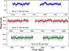 |
Fig. 1. Global TESS light curve of V479 And comprising three sectors (marked as 17, 57, and 84). Each sector is ≈28-day long. The original data has a cadence of 120 s. For better visualization, we binned the data to 600 points. The X-axes have similar lengths. |
The period analysis was performed using the Lomb–Scargle method (Lomb 1976; Scargle 1982), as implemented in the astropy.timeseries.LombScargle class (VanderPlas 2018). Fig. 2 shows the resulting power spectra. The first noteworthy characteristic is that the exact orbital frequency (Forb = 1.68325 d−1) corresponding to 0.594093 d), as determined from the spectroscopy (González-Buitrago et al. 2013), shows up in all sectors and is marked by a vertical green dotted line. The power is strongest in Sector 84 and weakest in 17 (the latter is very noisy and for clarity is not shown in Fig. 2). Meanwhile, the peak at twice the orbital frequency (2 × Forb = 3.3665 d−1) is also present in all sectors, but is much stronger in Sector 57, comparable to the orbital frequency in Sectors 84 and 17. False alarm probability (FAP) levels were derived for values of 0.1, 0.05, and 0.01, corresponding approximately to confidence levels of 90%, 95%, and 99%, respectively. These FAP thresholds were computed using the analytical prescription in the Astropy implementation. All relevant power peaks reach or exceed confidence levels, plotted as horizontal lines at a false alarm probability of 0.01 for each sector1. The power of Sectors 84 and 17 contains a multitude of other peaks exceeding FAP, but we did not explore them due to the low levels of variability in the data. We assume, nevertheless, that the frequencies strictly coinciding with the orbital and double orbital are not random.
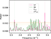 |
Fig. 2. Power spectra of V479 And for individual sectors, i.e., 57 (pink), and 84 (green). The horizontal lines indicate false alarm probability levels corresponding to 0.1 (dash-dotted; yellow), 0.05 (dotted; orange), and 0.01 (dashed; dark orange). The vertical dotted lines indicate meaningful frequencies: the red is the double orbital frequency, the green is the orbital frequency. |
The frequency corresponding to twice the orbital frequency is commonly attributed to the ellipsoidal variability produced by the Roche-Lobe-filling donor star. The amplitude of this variability is barely 0.018 mag, preventing us from getting a meaningful phase-folded light curve.
3.2. HST spectrum and chemical composition of V479 And
The COS spectrum of V479 And is presented in Fig. 3. No spectral features in absorption belonging to the underlying WD are detected. The spectrum is dominated by accretion-powered emission. Such spectra of magnetic CVs are rather common (e.g., Mauche et al. 1997; Schmidt & Stockman 2001). They are generally interpreted as a combination of accretion-heated photospheric spots, cyclotron-emitting shock spots, or emission from the accretion stream that is responsible for the UV continuum emission (Mauche et al. 1997). In a few cases, such as V1309 Ori, the extreme ratio of N Vλ1240/C IVλ1549 = 7.2 is suggestive of an overabundance of nitrogen in the gas stream (Schmidt & Stockman 2001). The spectrum of V479 And is also remarkable for the high intensity of N V and He IIλ1640 lines in comparison to very modest C IV. The strength of the He II line confirms that V479 And is a polar-type magnetic CV, deduced by observing repeating X-ray pulses with the orbital period (González-Buitrago et al. 2013). The X-ray/EUV emission from the magnetic pole provides sufficient energy to ionize He in the mass transfer streams and sometimes at the irradiated face of the donor star.
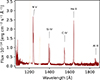 |
Fig. 3. HST COS UV spectrum of V479 And. The major emission lines are marked. The geocoronal lines are masked but displayed in a bleak color. |
The measured N V/C IV = 2.8 ratio (Table 1) is much larger than the value of 0.6 that is observed in the majority of CVs (e.g., the surveys of UV emission line ratios conducted by Mauche et al. 1997; Gänsicke et al. 2003; Godon & Sion 2023; Sanad 2011, and Toloza et al. 2023). There are currently about 30 CVs with such an inverted carbon-to-nitrogen ratio. They are all considered to have an evolved donor star that was formed from a binary containing a relatively massive secondary star with a CNO-dominated nuclear engine, which underwent an unstable thermal timescale mass transfer (TTMT) stage in its evolution (Schenker et al. 2002; Ge et al. 2010, 2020; El-Badry et al. 2021).
Fluxes and logarithmic line ratios for selected emission lines in the UV spectrum of V479 And.
The system CSS 120422:111127+571239 is one such binary with an evolved donor, on the short extreme of the orbital period distribution. Kennedy et al. (2015, their Fig. 12) illustrates perfectly how UV emission line ratios help to separate these objects from CVs formed according to a standard evolutionary scenario (i.e., those with unevolved main-sequence donor stars).
For resonance doublets such as N V λλ1238, 1242 and Si IV λλ1393, 1402, our COS spectra resolve the two components. We measured the flux of each component individually and then summed the fluxes to obtain the total doublet strength before computing line ratios and their logarithms. This approach ensures direct comparability with previous studies, many of which either used lower spectral resolution data or chose to report only combined doublet fluxes (e.g., Mauche et al. 1997; Gänsicke et al. 2003; Godon & Sion 2023; Sanad 2011; Toloza et al. 2023). While these works generally present non-logarithmic ratios, we follow the convention of Kennedy et al. (2015) and quote the logarithm of the flux ratios in Table 1, to compress the dynamic range and facilitate visual comparison with their diagnostic diagrams.
The composite spectrum of V479 And, comprised of the HST COS UV and the SDSS optical spectra, is shown in Fig. 4. In the ultraviolet spectrum, the continuum is dominated by emission from accretion processes, which effectively hide the white dwarf. By this we mean that no distinct spectral features attributable to the white dwarf photosphere are detected, because they are masked by the much stronger accretion–powered continuum.
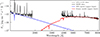 |
Fig. 4. Spectral energy distribution of V479 And comprised of the HST/COS ultraviolet spectrum (dark grey) and the SDSS optical spectrum (black). In blue and red are shown the upper limits for a white dwarf and a main-sequence star, respectively (see Section 3.2). The donor’s model assumes a distance of 1850 pc. The white dwarf model is scaled to the same distance, and both are plotted on an absolute flux scale. |
Ignoring the dominant UV contribution from accretion, we overplot a synthetic DA model spectrum of a white dwarf with M1 = 0.94 M⊙ (see Table B.1), computed from the 3D pure–hydrogen LTE grids including H2 molecular opacity (Tremblay et al. 2013, 2015), and scaled to a distance of 1850 pc. The adopted Teff = 38 000 K represents the hottest white dwarf still compatible with the short–wavelength edge of the HST spectrum, and thus sets an upper limit to the WD temperature. This corresponds to the maximum temperature at which the white dwarf can remain hidden in the composite spectrum. Using the mass–radius relation from the La Plata group2 (Camisassa et al. 2016), these parameters yield a radius of R1 = 0.0088 R⊙.
We subsequently performed a fit of the SDSS spectrum, fixing the WD mass to 0.94 M⊙, while allowing the donor’s Teff and mass to vary and constraining the donor radius to the Roche–lobe radius via Eq. (1). Using the grid of M-dwarf models by Allende Prieto et al. (2018), we obtained Md = 0.24 ± 0.10 M⊙, Rd = 0.84 ± 0.14 R⊙, and Teff = 5000 ± 170 K. These values should also be regarded as upper limits, since the contribution from accretion was not included in the fit. The donor’s model assumes Z = 0.13 and the same system distance of 1850 pc. Importantly, the parameters derived from this spectroscopic fit are consistent with the values obtained in Sect. 4.1 from photometry and Roche–geometry arguments, reinforcing the reliability of both approaches.
3.3. GTC IR spectrum of V1082 Sgr and chemical deviations
Although we could not obtain UV spectra of V1082 Sgr, we were able to get NIR spectra covering the full orbital cycle, revealing deviations of some key metal lines. To constrain the spectral type and luminosity class of the donor star, we compared the observed near-infrared spectra in the J, H, and K bands to a library of observed stellar spectral standards (Wallace & Hinkle 1997; Meyer et al. 1998; Wallace et al. 2000) spanning spectral types K0–K5 and luminosity classes V and IV. The comparison was performed by computing the reduced chi-square statistic, defined as χ2 = ∑i[(Fobs, i−Fstd, i)/σi]2, where Fobs, i and Fstd, i are the normalized flux densities of the observed and standard spectra, respectively, and σi represents the uncertainty in the observed flux at each wavelength point. All spectra were aligned in wavelength space using cross-correlation techniques and resampled to a common grid.
In the J and H bands, where dwarf and K1–K1.5 subgiant standards were available, the best fit in terms of minimum χ2 was obtained consistently for subgiant stars, despite small differences in effective temperature. For the J band, the minimum χ2 = 0.929 was found with a K1 IV standard, while nearby dwarf standards such as K0 V and K2 V yielded slightly higher values of χ2 = 1.185 and 1.060, respectively. In the H band, a K1.5 IV standard produced the best fit (χ2 = 6.89), compared to χ2 = 8.98 for the K2 V dwarf. These results favor a subgiant luminosity class for the donor. In the K band, where only a K0 IV standard was available for the subgiant class, the lowest χ2 was obtained using a K3 V dwarf template, suggesting a possible ambiguity in this band, likely due to the limited spectral coverage in available standards.
We measured radial velocities (RVs) of complexes of absorption lines in all three (J, H & K) bands, obtaining RVs presented in Fig. 5. They are concurring with the much more precise RV curve from high-resolution optical observations (Tovmassian et al. 2018a). Moreover, the Na I, Mg I lines, which we subsequently consider, follow the RV curve of the donor star, that is, do not have an interstellar or other exotic origin. A large fraction of NIR spectra are presented in Fig. 6. Significant lines from Rayner et al. (2009, Table 7) are marked, where the spectra of the corresponding standards are from the databases described in Wallace & Hinkle (1997), Meyer et al. (1998), and Wallace et al. (2000).
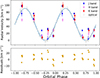 |
Fig. 5. Radial velocities measured from a complex of absorption lines in the J (blue), H (magenta), and K (red) bands of V1082 Sgr spectra. The curve fits the radial velocities obtained from high-resolution optical data shown as light-gray points in the upper panel. The residuals of J and K measurements from the radial velocity curve obtained from optical data are presented in the bottom panel. |
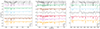 |
Fig. 6. IR spectra of V1082 Sgr. The spectra are co-added from five individual spectra taken evenly around orbital phases. They were shifted to zero velocity after measuring RVs before co-adding and normalizing. They are placed between K2 and later spectral-type standards because they best resemble the K2 spectral class, or slightly earlier if compared to IV luminosity class. |
The doublets Na I lines at λ22062.4 & 22089.7 Å show orbital variability, testifying that they originate in the atmosphere of the donor star. The zoom-in portions of the co-added and normalized spectra are shown in Fig. 7 together with standard stars, testifying that despite good accordance, there is a significant excess Na I and deficit of Mg I in the spectrum of V1082 Sgr. Na Iλ 22062.4 Å has an equivalent width EW = 2.65±0.05 Å, while it is expected for the K2 spectral type to be around 1.66 (Rayner et al. 2009).
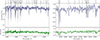 |
Fig. 7. Portions of the IR spectra of V1082 Sgr, emphasizing spectral lines in discordance with the corresponding standards, are presented in the upper panel. The residuals between the observed normalized spectrum and a K2 V type standard are shown in the bottom panels. Horizontal dotted orange lines mark the 3σ deviation level. Vertical dotted lines mark the deviating lines. |
The presence of an enhanced Na I doublet and a deficit of Mg I in V1082 Sgr also aligns with the findings of Harrison (2018), who noted that these chemical anomalies are common in hydrogen-deficient CV donor stars, particularly those with evolved secondaries. Harrison (2018, their Fig. 1) provided excellent evidence of an increasing strength of Na I doublet toward the hydrogen-poor synthetic spectra. The enhanced sodium abundance in V1082 Sgr is particularly striking, suggesting a donor star that has undergone substantial nuclear evolution, possibly due to its higher initial mass compared to typical CV donors.
The comparison with the CVs mentioned above, which harbor evolved secondaries, is telling. These systems exhibit evolved donor stars but do not show the same substantial sodium excess observed in V1082 Sgr. The absence of a similar Na I enhancement in these systems, despite their evolved nature, highlights the unusual and distinctive nature of the V1082 Sgr donor star. This divergence in chemical behavior suggests that the donor star in V1082 Sgr may have evolved through a different, possibly more extreme, evolutionary path, which could be linked to its higher initial mass or alternative evolutionary mechanisms, such as TTMT. Therefore, the sodium excess in V1082 Sgr strengthens the argument that its donor is not just evolved but may represent an alternative evolutionary pathway for CV evolution.
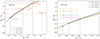 |
Fig. 8. Diagnostic diagrams of the R2–M2 relation for V1082 Sgr (left) and V479 And (right), assuming that the donor star fills its Roche lobe and accounting for the revised Gaia distance ranges. The methodology is described in Sect. 4.1. Horizontal dotted lines indicate the donor star radii (assuming spherical geometry) corresponding to the spectral class Teff needed to match the observed luminosity for different distances. Vertical lines mark the inferred donor masses. In the left panel, the solutions fall within the shaded green area. In contrast, solutions from the previous studies (labeled) illustrate that they are inconsistent with the revised distances adopted in this work. |
4. Basic parameters of the donor stars
We adopted improved Gaia DR3 distances in our following analyses. With these, we can derive the parameters of the donor stars in V1082 Sgr and V479 And.
4.1. Radii and masses
The mass of the donor star in a close binary system containing a WD can be estimated using a combination of Roche geometry, Kepler’s third law, and distance measurements. In systems where the donor star fills its Roche lobe and undergoes mass transfer, the size of the Roche lobe can be related to the mass ratio of the system, providing a means to estimate the donor’s mass. Here, we outline a methodology to estimate the donor star’s mass by constructing a mass–radius relation, leveraging the Eggleton approximation for the Roche lobe, and incorporating precise distances from the Gaia mission to derive absolute magnitudes and luminosities.
We used the volume–equivalent Roche–lobe radiusRL, ve3, i.e., the radius of a sphere having the same volume as the Roche lobe, computed with the Eggleton approximation (Eggleton 1983):
 (1)
(1)
where a is the binary separation and  is the mass ratio of the donor star to the WD. Assuming that the donor star fills its Roche lobe, we have R2 ≈ RL, where R2 is the donor radius.
The orbital separation, a, can be derived from Kepler’s third law as
 (2)
(2)
where G is the gravitational constant, M1 is the mass of the WD, M2 is the mass of the donor star, and Porb is the observed orbital period. From this, the orbital separation, a, can be computed for a given system.
To estimate the donor star’s mass, we construct a mass-radius relation for a range of WD masses. For each assumed M1, we calculate the Roche lobe radius RL as a function of M2, using the Eggleton formula and the corresponding binary separation a from Kepler’s law. This generates a set of curves in the R2-M2 plane for various assumed WD masses.
At the same time, the radius R2 of the donor star can be independently determined from its observed photometric properties. The donor star’s luminosity, L2; radius, R2; and effective temperature, T2, are related by the dimensionless relation:
 (3)
(3)
where L⊙, R⊙, and T⊙ are the solar luminosity, radius, and temperature, respectively. This allowed us to estimate the radius R2, based on the effective temperature, T2, derived from the spectrophotometric energy distribution fitting.
The luminosity, L, is derived from the absolute bolometric magnitude, Mbol, which we computed from the observed V-band apparent magnitude, the distance, the line-of-sight extinction, and the bolometric correction. The absolute visual magnitude is
 (4)
(4)
where mV is the observed apparent magnitude (not de-reddened), d is the distance in parsecs, and AV is the extinction in the V band. The bolometric magnitude is then
 (5)
(5)
In revisiting the distances adopted for the donor star analysis, we corrected the Gaia DR3 parallaxes for the zero point and recalculated the distances using both geometric and photogeometric estimates from Bailer-Jones et al. (2021a). For V479 And, the corrected parallax yields a distance of 1981 pc (ϖ = 0.505 mas), while the Bailer-Jones (Bailer-Jones et al. 2021b) estimates provide  pc (geometric) and
  pc (photogeometric). Applying an exponentially decreasing space density prior with a scale height of 250 pc, more appropriate for CVs above the period gap, we obtain a refined distance of
  pc. This is consistent with the Gaia DR3 spectrophotometric estimate (distance_gspphot = 1821 pc) and within the error range given the moderate ruwe of 1.0. Similarly, for V1082 Sgr, the corrected parallax (ϖ = 1.55 mas) gives 644 pc, fully consistent with the Bailer-Jones estimate (644 ± 7 pc geometric,
  pc photogeometric) and our prior-adjusted distance of 644 ± 8 pc. The radii-mass diagnostic diagram (Fig. 8) shows a range of solutions that account for the uncertainty in distance determination.
We used bolometric corrections corresponding to the spectral classes of the donor stars, adopting the tables of Flower (1996) and Eker & Bakış (2025). There is evidence that the bolometric corrections for K-type subgiants do not differ significantly from those of dwarfs; on the other hand, the choice of method for calculating BC introduces a larger source of uncertainty (Worthey & Lee 2011; Eker & Bakış 2025).
For V1082 Sgr, we adopted an apparent visual magnitude of mV ≃ 14.8 at minimum brightness, as measured by Tovmassian et al. (2016). For V479 And, no reliable direct photometric measurement of the donor exists. Instead, we used the same dataset as González-Buitrago et al. (2013), but estimated the donor’s contribution by scaling and subtracting template spectra of late-type standard stars until the absorption lines were optimally balanced and the continuum was smooth. This spectral-decomposition procedure yields an effective donor brightness equivalent to mV = 17.8 ± 0.1. These values should be regarded as upper limits to the donor brightness, since residual accretion light or the white dwarf may still contribute even in low states.
The intersection of the calculated donor radius R2 and the Roche lobe curves in the R2-M2 provides a solution for M2, the mass of the donor star. In Fig. 8, we present the Eggleton approximation for Roche lobe size for various M1 as a series of curves. The horizontal lines indicate possible R2 derived from the estimated effective T2, mV and the distance. We estimated the M2 range, assuming that the donor star fills its Roche lobe, and using the observed photometric brightness in the V band (González-Buitrago et al. 2013; Tovmassian et al. 2018a) of these two systems. However, the distance, the effective temperature, and even the brightness of the donor star are known to have large uncertainties. Hence, we have a series of R2 values that depend on the adopted observables. The vertical lines indicate M2 for different sets of parameters. While it is difficult to pinpoint the exact mass of the donor star, we can state unambiguously that the donor star is drastically smaller than an isolated main-sequence or pre-main-sequence star of corresponding temperature.
In the case of V1082 Sgr, we know well the brightness of the donor star, since the object often goes to very low states, in which the naked donor star is observed. The distance error is also relatively small. We get an M2 ≈ 0.22 − 0.24 M⊙ estimate for the donor mass (blue dots and dotted lines). Also shown are other solutions: the green point and dotted lines correspond to the proposed model of the object with an unevolved underfilling its Roche lobe donor star and for R2’s obtained with the models of Xu et al. (2019) models. They require much larger distances to the object than measured by Gaia.
There are no robust dynamical constraints on the masses of white dwarfs. For V1082 Sgr, indirect estimates from X-ray studies exist. Bernardini et al. (2013) derived M1 ≃ 0.64 M⊙ from the X-ray luminosity, while Xu et al. (2019) obtained a higher value of M1 ≃ 0.77 M⊙ by fitting the X-ray spectrum. Such differences are typical for X-ray based mass determinations in intermediate polars, which suffer from systematic uncertainties (e.g., Suleimanov et al. 2025) related to assumptions about accretion column structure, shock height, and partial covering absorption. We therefore consider these values as indicative only, rather than precise dynamical measurements.
For V479 And, the distance limits are wider, and the donor star’s temperature and brightness are deduced from the SED with significant uncertainties. All possible solutions, however, correspond to a donor mass of M2 < 0.31 M⊙. In both systems, the adopted MWD has no significant influence on our donor mass estimates. The ranges in Teff and mV of the secondary star are much larger than the modest differences introduced by the white dwarf mass.
4.2. Orbital Inclination
The orbital inclination can, in principle, be derived from the observed mass function,
 (6)
(6)
where K2 is the radial velocity semi-amplitude of the donor star. Observations fix the left-hand side, but the inclination angle i can only be determined if both stellar masses are specified.
Although one could, in principle, insert plausible average values of M1 and M2, there are no robust dynamical constraints on either system. We therefore adopted the values of M1 and M2 provided by our evolutionary models (see Sect. 5) to evaluate i. This exercise shows that both systems must be observed at relatively low inclinations (i ≃ 13°–18°). Moreover, V1082 Sgr is inferred to be slightly less inclined than V479 And.
While such low inclinations are a priori unlikely (∼3% for a single system and ∼0.1% for two), the observational constraints leave no alternative: both systems are best explained by low-inclination geometries.
5. Evolutionary models
We can use the parameters of the donors in V479 And and V1082 Sgr we derived in the previous sections to search for decent evolutionary models that can explain both extremely long-period CVs. We used the MESA code (version r15140 Paxton et al. 2011, 2013, 2015, 2018, 2019; Jermyn et al. 2023) for that and our assumptions for single star and binary evolution are described in the Appendix A. We were able to successfully find reasonable formation pathways for both V479 And and V1082 Sgr, which are provided in the Appendix B (Tables B.2 and B.1). The properties we predict in our modeling with MESA are compared to the observed in Table 2.
Predicted and observed parameters of V1082 Sgr and V479 And.
The evolution of the post-CE binaries leading to the present-day configurations of both V1082 Sgr and V479 And is rather similar. In particular, we can explain both systems with an initial post-CE binary having a WD mass of 0.8 M⊙ and a main-sequence star companion of mass 1.1 M⊙. However, as the observed orbital period of V1082 Sgr is longer than that of V479 And, the orbital period of the initial post-CE binary has to be longer for the former (3.5 d) in comparison to the latter (3 d). Therefore, the slight differences observed in both systems can be explained as the evolutionary stage of the companion of the WD at the onset of mass transfer. Right after CE evolution, the orbital period is too long for the companion of the WD to fill its Roche lobe as a main-sequence star. Therefore, it has to first become a subgiant before eventually filling its Roche lobe due to the expansion driven by hydrogen shell burning, as illustrated in Figs. 9 and 10. This detached post-CE evolution takes several Gyr (Tables B.2 and B.1).
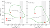 |
Fig. 9. Post-CE evolution of the luminosity with the effective temperature of the donor in V1082 Sgr (left panel) and V479 And (right panel). The red solar symbol indicates the properties at the moment the WD was formed (i.e., just after CE evolution), and the thick red cross indicates the properties at the moment the orbital period is the same as observed. The thick grey vertical strip corresponds to the properties derived from observations. More details are provided in Sect. 5. |
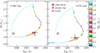 |
Fig. 10. Post-CE evolution of the radius with the effective temperature of the donor in V1082 Sgr (left panel) and V479 And (right panel), color coded by its mass. The red solar symbol indicates the properties at the moment the WD was formed (i.e. just after CE evolution) and the thick red cross the properties at the moment the orbital period is the same as observed. The grey star corresponds to the properties derived from observations. More details are provided in Sect. 5. |
After the onset of mass transfer, although the donor star can maintain its hydrostatic equilibrium, it must sacrifice its thermal equilibrium in response to Roche-lobe-filling mass transfer. This causes the mass-loss timescale to be comparable to the thermal (Kelvin–Helmholtz) timescale of the donor star. During thermal timescale mass transfer, the mass transfer rates are so high (≳10−7 M⊙ yr−1) that hydrogen can be burnt steadily on the surface of the WD, causing an increase in its mass, as illustrated in Figs. 11 and 12. As the mass of the donor star decreases, at some point the mass-loss timescale starts to increase and becomes greater than the thermal timescale of the donor star. When this happens, the donor can reestablish thermal equilibrium, and the thermal timescale mass transfer ends.
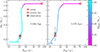 |
Fig. 11. Post-CE evolution of the donor mass with the orbital period, color coded by the WD mass, for V1082 Sgr (left panel) and V479 And (right panel). The red solar symbol indicates the moment at which the white dwarf was formed, while the thick red cross the properties at the moment the orbital period is the same as the observation. More details are provided in Sect. 5. |
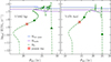 |
Fig. 12. Post-CE evolution of the mass transfer rate (green dot-dashed line) with the orbital period for V1082 Sgr (left panel) and V479 And (right panel). The thick red cross indicates the properties at the moment the orbital period is the same as the observation. The purple line corresponds to the critical mass transfer rate Ṁstable above which hydrogen can burn steadily in a shell. The blue line corresponds to the maximum burning rate Ṁred-giant such that, for higher mass transfer rates, not all the transferred mass is accreted. The non-accreted mass piles up above the WD and is eventually lost from its vicinity in the form of fast winds similar to those of red giants. More details are provided in Sect. 5. |
From this point on, the mass transfer rate decreases as the donor mass decreases since the evolution becomes driven by magnetic braking, and hydrogen burning on the surface of the WD is unstable, leading to cyclic nova eruptions. The accreted matter is then ejected from the binary due to these repetitive nova eruptions, which keep the WD mass roughly constant. Meanwhile, the binary evolves towards shorter periods as the donor mass decreases. At present, the binary has properties comparable to those observed (Table 2).
6. Discussion
A new data set was collected on the two extremely long period CVs V1082 Sgr and V479 including TESS-photometry, UV and IR spectroscopy. Combined with the circular polarimetry recently reported by Lima et al. (2025), the data set allowed us to better interpret the controversial nature of these systems and carry out detailed evolutionary models to account for their characteristics.
The TESS data helped to reveal periodic variability in the light curves of V479 And. The double orbital frequency, prominent in only one block of TESS data, is evidence of a double-hump light curve per orbital period, characteristic of ellipsoidal distortion of the Roche-lobe-filling donor star. The donor star is a significant contributor to light at the near-IR wavelength, corresponding to the TESS bandpass. However, a small amplitude of variability ≤1.5% results either from a star not completely filling its Roche Lobe, or a very small angle of the binary orbit. We show in Section 4.2 that the inclination angle is indeed small from other considerations.
The UV spectrum of V479 And revealed an anomalously high N V/C IV emission-line flux ratios. This is a common feature among CVs with evolved donors (Gänsicke et al. 2003). A more extensive selection of such systems with nuclearly evolved donors is presented by Kennedy et al. (2015). V479 And with N V/C IV = 2.8 falls within a cluster of CVs of inverted line ratio systems BY Cam, EY Cyg, BZ UMa, EI Psc, and AE Aqr (Kennedy et al. 2015, their Fig. 12). It confirms that V479 And had an alternative evolutionary path in comparison to typical CV evolution with unevolved donor stars.
Meanwhile, the circular polarization data of V1082 Sgr revealed the presence of significant power at f = 12.352 d−1 (i.e., 1.943 h, Lima et al. 2025). By detecting the circular polarization modulated with an ≈0.1× Porb, it was firmly established that V1082 Sgr is indeed an intermediate polar with the third longest known spin period. This, alone, essentially invalidates the previously proposed mass transfer model governed by the coupling magnetic fields (Tovmassian et al. 2016). That model already had difficulties explaining a high mass transfer rate from the stellar wind. This system is better explained by assuming it is semi-detached, with mass transfer occurring through the L1 point from the Roche-filling secondary.
In addition, the IR spectroscopy showed an anomalous chemical composition of the donor star in V1082 Sgr, identical to some other CVs (Harrison 2016). Much like the similarly divergent chemical composition of accretion material of V479 And it is strong proof that V1082 Sgr went through a TTMT evolutionary episode, as proposed by Xu et al. (2019).
We revisited the basic binary parameters of both systems. We showed in Sect. 4.1 that both V479 And and V1082 Sgr contain radically lightweight donor stars. This confirms and strengthens the argument that their secondary stars are not only nuclearly evolved but also have lost most of their envelopes. It makes their further evolution even more intriguing.
The scenario according to which the companion of V1082 Sgr has evolved off the main sequence and lost ∼0.5 − 2.0 M⊙ of its mass was initially proposed by Xu et al. (2019) for V1082 Sgr. According to their numerical calculations, the companion appears as a K-type star with an effective temperature of 4660–5100 K and mass ranging from M2 = 0.45 − 0.568 M⊙. However, this is inconsistent with the parameters of the donor star we derived here (Fig. 8). We calculated evolutionary models, achieving a satisfactory agreement between the predicted and observed properties of the donor stars, specifically their masses, radii, and luminosities.
After CE evolution, the evolution of the binary can be driven by either nuclear evolution, or angular momentum loss due to magnetic braking, or a combination of both. While the nuclear timescale evolution is relatively well understood, the same cannot be said about magnetic braking. The strength and main dependencies of magnetic braking on stellar parameters (e.g. mass, structure, magnetic field, and evolutionary stage) are highly uncertain. Despite that, there has been progress in understanding magnetic braking in the past years.
Regarding unevolved main-sequence stars, there is growing evidence that magnetic braking saturates (e.g., Reiners et al. 2009), that is, beyond a certain rotation rate, the activity becomes independent of the rotation rate. This means that the angular momentum loss due to magnetic braking becomes only weakly dependent on the rotation rate (e.g., Chaboyer et al. 1995). This also occurs for stars in binary main-sequence stars as well as detached and semi-detached post-CE WD binaries (e.g., El-Badry et al. 2022; Belloni et al. 2024; Barraza-Jorquera et al. 2025). Additionally, magnetic braking is much more efficient for stars with a radiative core and a convective envelope in comparison to fully convective stars (Belloni et al. 2024; Schreiber et al. 2024; Barraza-Jorquera et al. 2025).
On the other hand, predictions for evolved main-sequence stars and subgiants are in better agreement with observations when magnetic braking is assumed to be much stronger in comparison to unevolved main-sequence stars. For instance, the characteristics of the populations of transient and persistent neutron star low-mass X-ray binaries, transitional millisecond pulsar binaries, and ultra-compact X-ray binaries are much better explained by assuming the CARB (Van & Ivanova 2019) model (or other similar prescriptions) for strong magnetic braking (e.g. Van et al. 2019; Van & Ivanova 2019, 2021; Deng et al. 2021; Chen et al. 2021; Shahbaz et al. 2022; Wei et al. 2023; Castro Segura et al. 2024; Echeveste et al. 2024; Cui & Li 2024; Yang & Li 2024; Kar et al. 2025; Yang et al. 2025). Similarly, the fine-tuning problem related to the formation of ultra-compact X-ray binaries, detached close millisecond pulsar binaries, and AM CVn binaries can be solved by assuming strong magnetic braking (e.g. Chen et al. 2021; Soethe & Kepler 2021; Belloni & Schreiber 2023b). Here, we provide further evidence for strong magnetic braking acting on subgiants, which is required to explain the orbital periods of both V479 And and V1082 Sgr, whose donor stars have undergone CNO processing.
We performed new evolutionary calculations adopting the CARB model (Van & Ivanova 2019) for magnetic braking. Due to the high AML rates predicted by this model, the binary evolution after CE evolution is convergent, despite the donor star having already evolved into a subgiant. The introduction of the CARB in our modeling is the noteworthy difference between our models and those calculated by Xu et al. (2019).
Despite the success of the CARB model when applied to nuclear evolved donors in accreting compact objects, it also faces problems. For example, Fan et al. (2024) showed that the CARB model cannot explain the orbital-period derivative of two neutron star low-mass X-ray binaries (SAX J1748.9-2021 and XTE J1710-281) and two black hole low-mass X-ray binaries (A0620-00 and Nova Muscae 1991). More recently, Belloni et al. (2025) showed that the paradoxical system SDSS J1257+5428, which is a double WD binary with an orbital period of only 4.56 h, can only be explained if the post-CE evolution is convergent, requiring an AML rate that is ∼100 times higher than the predicted by the CARB model. That being said, although the CARB model is a promising model for nuclear evolved stars, it still needs improvements to account for several difficulties.
7. Conclusions
We have collected a wealth of new data on two unusual CVs, V1082 Sgr and V479 And, with extremely long orbital periods, 20.8 and 14.3 hours, respectively, compared to most CVs. We have used these data to determine the properties of the secondary stars in the two systems. As detailed in Table 2, both have secondary star masses of about 0.24 M⊙, and effective temperatures of about 5100 K. V479 And has a smaller donor star radius of about 0.85 R⊙, while V1082 Sgr is about 1.1 R⊙, as a result of its longer period. Curiously, we find that both objects have a very low inclination. This explains the low amplitude of the double-hump variability of the light curve of V479 And (TESS) data described here and non-detection in V1082 Sgr (Tovmassian et al. 2018b).
A recent study has established that V1082 Sgr hosts a moderate strength magnetic white dwarf and is classified as an intermediate polar (Lima et al. 2025). For V479 And, we report the presence of an intense He II line in its UV spectrum, which is generally regarded as indirect evidence of a strongly magnetic white dwarf, consistent with the conclusion of González-Buitrago et al. (2013) who identified repetitive X-ray flashes as a signature of a polar. Our analysis shows that, despite these differences in magnetic properties and classification, both binaries appear to follow a similar evolutionary trajectory. This suggests that the secular evolution of these long-period CVs is not strongly dependent on whether the accreting white dwarf is an intermediate polar or a polar candidate.
Furthermore, we find that the donor stars in both systems have atypical chemical compositions and significantly lower masses than most objects in their spectral classes. These differences in characteristics compared to most CVs lead us to conclude that a brief and unstable phase of mass transfer has been involved in the evolution of both systems. Our evolutionary models explain the diverging chemical composition of the emitting gas in these systems compared to the normal CVs. By simulating binary evolution models that assume strong magnetic braking, we achieved a better agreement with observations, considering the measured distances, luminosities, and radii of donor stars determined independently from observations, in comparison to previous models.
Our findings provide further evidence for stronger magnetic braking acting on subgiants in close-orbit accreting compact objects in comparison to unevolved main-sequence stars. Among accreting white dwarfs, they might significantly contribute to the population of close binary white dwarfs. To further test this hypothesis, similarly detailed investigations of other extremely long-period systems are required.
We note that these thresholds are commonly referred to as ‘false alarm probabilities’ in the literature (e.g., Press et al. 1992), although they do not strictly represent false detection rates in a Bayesian sense.
We refer to RL, ve simply as the Roche lobe radius, RL, further in the text.
Acknowledgments
We thank the referee of this paper, Dr Albert Bruch, for his detailed reading and insightful comments, which enhanced the clarity and rigor of the manuscript. GT was supported by grants IN113723, IN109723 from the Programa de Apoyo a Proyectos de Investigación e Innovación Tecnológica (PAPIIT). DB acknowledges support from the São Paulo Research Foundation (FAPESP), Brazil, Process Numbers #2024/03736-2 and #2025/00817-4. This project has received funding from the European Research Council (ERC) under the European Union’s Horizon 2020 research and innovation programme (Grant agreement No. 101020057). This research was supported by Deutsche Forschungsgemeinschaft (DFG, German Research Foundation) under Germany’s Excellence Strategy – EXC 2121 “Quantum Universe” – 390833306. Co-funded by the European Union (ERC, CompactBINARIES, 101078773) Views and opinions expressed are, however, those of the author(s) only and do not necessarily reflect those of the European Union or the European Research Council. Neither the European Union nor the granting authority can be held responsible for them. Partial support for KSL’s effort on the project was provided by NASA through grant numbers HST-GO-16489 and HST-GO-16659 from the Space Telescope Science Institute, which is operated by AURA, Inc., under NASA contract NAS 5-26555. RIH acknowledges support from NASA through grant number HST-GO-15454 from the Space Telescope Science Institute, which is operated by AURA, Inc., under NASA contract NAS 5-26555.
References
- Ahn, C. P., Alexandroff, R., Allende Prieto, C., et al. 2012, ApJS, 203, 21 [Google Scholar]
- Alam, S., Albareti, F. D., Allende Prieto, C., et al. 2015, ApJS, 219, 12 [Google Scholar]
- Allende Prieto, C., Koesterke, L., Hubeny, I., et al. 2018, A&A, 618, A25 [NASA ADS] [CrossRef] [EDP Sciences] [Google Scholar]
- Anders, E. H., & Pedersen, M. G. 2023, Galaxies, 11, 56 [NASA ADS] [CrossRef] [Google Scholar]
- Angulo, C., Arnould, M., Rayet, M., et al. 1999, Nucl. Phys. A, 656, 3 [Google Scholar]
- Bailer-Jones, C. A. L., Rybizki, J., Fouesneau, M., Demleitner, M., & Andrae, R. 2021a, AJ, 161, 147 [Google Scholar]
- Bailer-Jones, C. A. L., Rybizki, J., Fouesneau, M., Demleitner, M., & Andrae, R. 2021b, VizieR On-line Data Catalog: I/352 [Google Scholar]
- Barraza-Jorquera, J. A., Schreiber, M. R., & Belloni, D. 2025, A&A, 696, A92 [NASA ADS] [CrossRef] [EDP Sciences] [Google Scholar]
- Belloni, D., & Schreiber, M. R. 2023a, in Handbook of X-ray and Gamma-ray Astrophysics, eds. C. Bambi, & A. Santangelo (Singapore: Springer Nature Singapore), 1 [Google Scholar]
- Belloni, D., & Schreiber, M. R. 2023b, A&A, 678, A34 [NASA ADS] [CrossRef] [EDP Sciences] [Google Scholar]
- Belloni, D., Schreiber, M. R., Zorotovic, M., et al. 2018, MNRAS, 478, 5639 [Google Scholar]
- Belloni, D., Schreiber, M. R., Moe, M., El-Badry, K., & Shen, K. J. 2024, A&A, 682, A33 [NASA ADS] [CrossRef] [EDP Sciences] [Google Scholar]
- Belloni, D., Schreiber, M. R., & El-Badry, K. 2025, A&A, 697, A100 [NASA ADS] [CrossRef] [EDP Sciences] [Google Scholar]
- Bernardini, F., de Martino, D., Mukai, K., et al. 2013, MNRAS, 435, 2822 [NASA ADS] [CrossRef] [Google Scholar]
- Buchler, J. R., & Yueh, W. R. 1976, ApJ, 210, 440 [NASA ADS] [CrossRef] [Google Scholar]
- Camisassa, M. E., Althaus, L. G., Córsico, A. H., et al. 2016, ApJ, 823, 158 [CrossRef] [Google Scholar]
- Cassisi, S., Potekhin, A. Y., Pietrinferni, A., Catelan, M., & Salaris, M. 2007, ApJ, 661, 1094 [NASA ADS] [CrossRef] [Google Scholar]
- Castro Segura, N., Knigge, C., Matthews, J. H., et al. 2024, MNRAS, 527, 2508 [Google Scholar]
- Chaboyer, B., Demarque, P., & Pinsonneault, M. H. 1995, ApJ, 441, 865 [Google Scholar]
- Chen, H.-L., Tauris, T. M., Han, Z., & Chen, X. 2021, MNRAS, 503, 3540 [NASA ADS] [CrossRef] [Google Scholar]
- Chugunov, A. I., Dewitt, H. E., & Yakovlev, D. G. 2007, Phys. Rev. D, 76, 025028 [NASA ADS] [CrossRef] [Google Scholar]
- Cui, Z., & Li, X.-D. 2024, MNRAS, 533, 3637 [Google Scholar]
- Cyburt, R. H., Amthor, A. M., Ferguson, R., et al. 2010, ApJS, 189, 240 [NASA ADS] [CrossRef] [Google Scholar]
- Deng, Z.-L., Li, X.-D., Gao, Z.-F., & Shao, Y. 2021, ApJ, 909, 174 [NASA ADS] [CrossRef] [Google Scholar]
- Echeveste, M., Novarino, M. L., Benvenuto, O. G., & De Vito, M. A. 2024, MNRAS, 530, 4277 [NASA ADS] [CrossRef] [Google Scholar]
- Eggleton, P. P. 1983, ApJ, 268, 368 [Google Scholar]
- Eker, Z., & Bakış, V. 2025, Phys. Astron. Rep., 3, 43 [Google Scholar]
- El-Badry, K., Rix, H.-W., Quataert, E., Kupfer, T., & Shen, K. J. 2021, MNRAS, 508, 4106 [CrossRef] [Google Scholar]
- El-Badry, K., Conroy, C., Fuller, J., et al. 2022, MNRAS, 517, 4916 [NASA ADS] [CrossRef] [Google Scholar]
- Fan, Y.-N., Shao, Y., & Chen, W.-C. 2024, ApJ, 976, 210 [Google Scholar]
- Ferguson, J. W., Alexander, D. R., Allard, F., et al. 2005, ApJ, 623, 585 [Google Scholar]
- Fitzpatrick, E. L. 1999, PASP, 111, 63 [Google Scholar]
- Flower, P. J. 1996, ApJ, 469, 355 [NASA ADS] [CrossRef] [Google Scholar]
- Freedman, R. S., Marley, M. S., & Lodders, K. 2008, ApJS, 174, 504 [NASA ADS] [CrossRef] [Google Scholar]
- Freedman, R. S., Lustig-Yaeger, J., Fortney, J. J., et al. 2014, ApJS, 214, 25 [CrossRef] [Google Scholar]
- Freytag, B., Ludwig, H. G., & Steffen, M. 1996, A&A, 313, 497 [NASA ADS] [Google Scholar]
- Fuller, G. M., Fowler, W. A., & Newman, M. J. 1985, ApJ, 293, 1 [NASA ADS] [CrossRef] [Google Scholar]
- Gänsicke, B. T., Szkody, P., de Martino, D., et al. 2003, ApJ, 594, 443 [NASA ADS] [CrossRef] [Google Scholar]
- Gänsicke, B. T., Dillon, M., Southworth, J., et al. 2009, MNRAS, 397, 2170 [NASA ADS] [CrossRef] [Google Scholar]
- Garzón, F., Balcells, M., Gallego, J., et al. 2022, A&A, 667, A107 [CrossRef] [EDP Sciences] [Google Scholar]
- Ge, H., Hjellming, M. S., Webbink, R. F., Chen, X., & Han, Z. 2010, ApJ, 717, 724 [NASA ADS] [CrossRef] [Google Scholar]
- Ge, H., Webbink, R. F., & Han, Z. 2020, ApJS, 249, 9 [NASA ADS] [CrossRef] [Google Scholar]
- Gehrels, N., Chincarini, G., Giommi, P., et al. 2004, ApJ, 611, 1005 [Google Scholar]
- Godon, P., & Sion, E. M. 2023, ApJ, 950, 139 [Google Scholar]
- González-Buitrago, D., Tovmassian, G., Zharikov, S., et al. 2013, A&A, 553, A28 [Google Scholar]
- Green, G. M., Schlafly, E., Zucker, C., Speagle, J. S., & Finkbeiner, D. 2019, ApJ, 887, 93 [NASA ADS] [CrossRef] [Google Scholar]
- Harrison, T. E. 2016, ApJ, 833, 14 [NASA ADS] [CrossRef] [Google Scholar]
- Harrison, T. E. 2018, ApJ, 861, 102 [NASA ADS] [CrossRef] [Google Scholar]
- Henyey, L., Vardya, M. S., & Bodenheimer, P. 1965, ApJ, 142, 841 [Google Scholar]
- Herwig, F. 2000, A&A, 360, 952 [NASA ADS] [Google Scholar]
- Iglesias, C. A., & Rogers, F. J. 1993, ApJ, 412, 752 [Google Scholar]
- Iglesias, C. A., & Rogers, F. J. 1996, ApJ, 464, 943 [NASA ADS] [CrossRef] [Google Scholar]
- Inight, K., Gänsicke, B. T., Breedt, E., et al. 2023, MNRAS, 524, 4867 [NASA ADS] [CrossRef] [Google Scholar]
- Inight, K., Gänsicke, B. T., Schwope, A., et al. 2025, MNRAS, 536, 1057 [Google Scholar]
- Irwin, A. W. 2004, The FreeEOS Code for Calculating the Equation of State for Stellar Interiors, http://freeeos.sourceforge.net/ [Google Scholar]
- Istrate, A. G., Tauris, T. M., & Langer, N. 2014, A&A, 571, A45 [NASA ADS] [CrossRef] [EDP Sciences] [Google Scholar]
- Itoh, N., Hayashi, H., Nishikawa, A., & Kohyama, Y. 1996, ApJS, 102, 411 [NASA ADS] [CrossRef] [Google Scholar]
- Jermyn, A. S., Schwab, J., Bauer, E., Timmes, F. X., & Potekhin, A. Y. 2021, ApJ, 913, 72 [NASA ADS] [CrossRef] [Google Scholar]
- Jermyn, A. S., Bauer, E. B., Schwab, J., et al. 2023, ApJS, 265, 15 [NASA ADS] [CrossRef] [Google Scholar]
- José, J., Shore, S. N., & Casanova, J. 2020, A&A, 634, A5 [EDP Sciences] [Google Scholar]
- Joyce, M., & Tayar, J. 2023, Galaxies, 11, 75 [NASA ADS] [CrossRef] [Google Scholar]
- Kar, A., Ojha, P., & Bhattacharyya, S. 2025, ApJ, 980, 51 [Google Scholar]
- Kennedy, M., Garnavich, P., Callanan, P., et al. 2015, ApJ, 815, 131 [NASA ADS] [CrossRef] [Google Scholar]
- King, A. R., & Kolb, U. 1995, ApJ, 439, 330 [NASA ADS] [CrossRef] [Google Scholar]
- Knigge, C., Baraffe, I., & Patterson, J. 2011, ApJS, 194, 28 [Google Scholar]
- Langanke, K., & Martínez-Pinedo, G. 2000, Nucl. Phys. A, 673, 481 [NASA ADS] [CrossRef] [Google Scholar]
- Lima, I. J., Tovmassian, G., Rodrigues, C. V., et al. 2025, ApJ, 984, 152 [Google Scholar]
- Lomb, N. R. 1976, Ap&SS, 39, 447 [Google Scholar]
- Mauche, C. W., Lee, Y. P., & Kallman, T. R. 1997, ApJ, 477, 832 [Google Scholar]
- Maza, J., & Gonzalez, L. E. 1983, IAU Circ., 3854, 2 [Google Scholar]
- McAllister, M., Littlefair, S. P., Parsons, S. G., et al. 2019, MNRAS, 486, 5535 [NASA ADS] [CrossRef] [Google Scholar]
- Meyer, M. R., Edwards, S., Hinkle, K. H., & Strom, S. E. 1998, ApJ, 508, 397 [CrossRef] [Google Scholar]
- Ochsenbein, F. 1996, The VizieR database of astronomical catalogues (CDS, Centre de Données astronomiques de Strasbourg) [Google Scholar]
- Oda, T., Hino, M., Muto, K., Takahara, M., & Sato, K. 1994, At. Data Nucl. Data Tables, 56, 231 [NASA ADS] [CrossRef] [Google Scholar]
- Pala, A. F., Gänsicke, B. T., Breedt, E., et al. 2020, MNRAS, 494, 3799 [Google Scholar]
- Pala, A. F., Gänsicke, B. T., Belloni, D., et al. 2022, MNRAS, 510, 6110 [NASA ADS] [CrossRef] [Google Scholar]
- Paxton, B., Bildsten, L., Dotter, A., et al. 2011, ApJS, 192, 3 [Google Scholar]
- Paxton, B., Cantiello, M., Arras, P., et al. 2013, ApJS, 208, 4 [Google Scholar]
- Paxton, B., Marchant, P., Schwab, J., et al. 2015, ApJS, 220, 15 [Google Scholar]
- Paxton, B., Schwab, J., Bauer, E. B., et al. 2018, ApJS, 234, 34 [NASA ADS] [CrossRef] [Google Scholar]
- Paxton, B., Smolec, R., Schwab, J., et al. 2019, ApJS, 243, 10 [Google Scholar]
- Potekhin, A. Y., & Chabrier, G. 2010, Contrib. Plasma Phys., 50, 82 [NASA ADS] [CrossRef] [Google Scholar]
- Press, W. H., Teukolsky, S. A., Vetterling, W. T., & Flannery, B. P. 1992, The Art of Scientific Computing (Cambridge: University Press) [Google Scholar]
- Rappaport, S., Verbunt, F., & Joss, P. C. 1983, ApJ, 275, 713 [Google Scholar]
- Rayner, J. T., Cushing, M. C., & Vacca, W. D. 2009, ApJS, 185, 289 [Google Scholar]
- Reimers, D. 1975, Mem. Soc. R. Sci. Liege., 8, 369 [Google Scholar]
- Reiners, A., Basri, G., & Browning, M. 2009, ApJ, 692, 538 [NASA ADS] [CrossRef] [Google Scholar]
- Ricker, G. R., Winn, J. N., Vanderspek, R., et al. 2015, J. Astron. Telesc. Instrum. Syst., 1, 014003 [Google Scholar]
- Ritter, H. 1988, A&A, 202, 93 [NASA ADS] [Google Scholar]
- Rogers, F. J., & Nayfonov, A. 2002, ApJ, 576, 1064 [Google Scholar]
- Roming, P. W. A., Kennedy, T. E., Mason, K. O., et al. 2005, Space Sci. Rev., 120, 95 [Google Scholar]
- Sanad, M. R. 2011, New Astron., 16, 19 [Google Scholar]
- Saumon, D., Chabrier, G., & van Horn, H. M. 1995, ApJS, 99, 713 [NASA ADS] [CrossRef] [Google Scholar]
- Scargle, J. D. 1982, ApJ, 263, 835 [Google Scholar]
- Schaller, G., Schaerer, D., Meynet, G., & Maeder, A. 1992, A&AS, 96, 269 [Google Scholar]
- Schenker, K., King, A. R., Kolb, U., Wynn, G. A., & Zhang, Z. 2002, MNRAS, 337, 1105 [NASA ADS] [CrossRef] [Google Scholar]
- Schlegel, D. J., Finkbeiner, D. P., & Davis, M. 1998, ApJ, 500, 525 [Google Scholar]
- Schmidt, G. D., & Stockman, H. S. 2001, ApJ, 548, 410 [Google Scholar]
- Schreiber, M. R., Zorotovic, M., & Wijnen, T. P. G. 2016, MNRAS, 455, L16 [NASA ADS] [CrossRef] [Google Scholar]
- Schreiber, M. R., Belloni, D., & Schwope, A. D. 2024, A&A, 682, L7 [NASA ADS] [CrossRef] [EDP Sciences] [Google Scholar]
- Schwope, A. D., Brunner, H., Hambaryan, V., & Schwarz, R. 2002, ASP Conf. Ser., 261, 102 [NASA ADS] [Google Scholar]
- Shahbaz, T., González-Hernández, J. I., Breton, R. P., et al. 2022, MNRAS, 513, 71 [NASA ADS] [CrossRef] [Google Scholar]
- Shaw, A. W., Heinke, C. O., Maccarone, T. J., et al. 2020, MNRAS, 492, 4344 [Google Scholar]
- Smee, S. A., Gunn, J. E., Uomoto, A., et al. 2013, AJ, 146, 32 [Google Scholar]
- Soethe, L. T. T., & Kepler, S. O. 2021, MNRAS, 506, 3266 [NASA ADS] [CrossRef] [Google Scholar]
- Suleimanov, V. F., Ducci, L., Doroshenko, V., & Werner, K. 2025, A&A, 700, A180 [NASA ADS] [CrossRef] [EDP Sciences] [Google Scholar]
- Templeton, M. R. 2007, AAVSO Alert Notice, 349 [Google Scholar]
- Timmes, F. X., & Swesty, F. D. 2000, ApJS, 126, 501 [NASA ADS] [CrossRef] [Google Scholar]
- Toloza, O., Gänsicke, B. T., Guzmán-Rincón, L. M., et al. 2023, MNRAS, 523, 305 [CrossRef] [Google Scholar]
- Tovmassian, G., González-Buitrago, D., Zharikov, S., et al. 2016, ApJ, 819, 75 [Google Scholar]
- Tovmassian, G., González, J. F., Hernández, M. S., et al. 2018a, ApJ, 869, 22 [Google Scholar]
- Tovmassian, G., Szkody, P., Yarza, R., & Kennedy, M. 2018b, ApJ, 863, 47 [Google Scholar]
- Tremblay, P. E., Ludwig, H. G., Steffen, M., & Freytag, B. 2013, A&A, 559, A104 [NASA ADS] [CrossRef] [EDP Sciences] [Google Scholar]
- Tremblay, P. E., Gianninas, A., Kilic, M., et al. 2015, ApJ, 809, 148 [NASA ADS] [CrossRef] [Google Scholar]
- Van, K. X., & Ivanova, N. 2019, ApJ, 886, L31 [NASA ADS] [CrossRef] [Google Scholar]
- Van, K. X., & Ivanova, N. 2021, ApJ, 922, 174 [NASA ADS] [CrossRef] [Google Scholar]
- Van, K. X., Ivanova, N., & Heinke, C. O. 2019, MNRAS, 483, 5595 [NASA ADS] [CrossRef] [Google Scholar]
- VanderPlas, J. T. 2018, ApJS, 236, 16 [Google Scholar]
- Vanderspek, R., Doty, J., Fausnaugh, M., et al. 2018, TESS Instrument Handbook, Tech. rep. (MIT Kavli Institute for Astrophysics and Space Research) [Google Scholar]
- Wallace, L., & Hinkle, K. 1997, ApJS, 111, 445 [NASA ADS] [CrossRef] [Google Scholar]
- Wallace, L., Meyer, M. R., Hinkle, K., & Edwards, S. 2000, ApJ, 535, 325 [NASA ADS] [CrossRef] [Google Scholar]
- Warner, B. 1995, Camb. Astrophys. Ser., 28 [Google Scholar]
- Wei, N., Jiang, L., & Chen, W.-C. 2023, A&A, 679, A74 [NASA ADS] [CrossRef] [EDP Sciences] [Google Scholar]
- Wiktorowicz, G., Belczynski, K., & Maccarone, T. 2014, in Binary Systems, their Evolution and Environments, 37 [Google Scholar]
- Wolf, W. M., Bildsten, L., Brooks, J., & Paxton, B. 2013, ApJ, 777, 136 [Google Scholar]
- Worthey, G., & Lee, H.-C. 2011, ApJS, 193, 1 [CrossRef] [Google Scholar]
- Xu, X., Shao, Y., & Li, X.-D. 2019, MNRAS, 489, 3031 [NASA ADS] [CrossRef] [Google Scholar]
- Yang, H.-R., & Li, X.-D. 2024, ApJ, 974, 298 [Google Scholar]
- Yang, X.-P., Xu, K., Gao, Z.-F., Jiang, L., & Chen, W.-C. 2025, ApJ, 986, 219 [Google Scholar]
Appendix A: Secular evolution modeling of V479 And and V1082 Sgr
We used the version r15140 of the MESA code (Paxton et al. 2011, 2013, 2015, 2018, 2019; Jermyn et al. 2023) to calculate post-common-envelope (CE) binary evolution from the moment just after CE evolution onward. We describe here our assumptions for single star and binary evolution, which are summarized in Table A.1. For reference, our approach follows closely that by Belloni & Schreiber (2023b)4.
The MESA equation of state is a blend of the OPAL (Rogers & Nayfonov 2002), SCVH (Saumon et al. 1995), FreeEOS (Irwin 2004), HELM (Timmes & Swesty 2000), PC (Potekhin & Chabrier 2010) and Skye (Jermyn et al. 2021) equations of state. Nuclear reaction rates are a combination of rates from NACRE (Angulo et al. 1999), JINA REACLIB (Cyburt et al. 2010), plus additional tabulated weak reaction rates (Fuller et al. 1985; Oda et al. 1994; Langanke & Martínez-Pinedo 2000). Screening is included via the prescription of Chugunov et al. (2007) and thermal neutrino loss rates are from Itoh et al. (1996). Electron conduction opacities are from Cassisi et al. (2007) and radiative opacities are primarily from OPAL (Iglesias & Rogers 1993, 1996), with high-temperature Compton-scattering dominated regime calculated using the equations of Buchler & Yueh (1976).
We varied the metallicity by adopting the values from Z = 0.005 to 0.025, in step of 0.005, to account for sub-solar, solar, and super-solar metallicity models. We assumed the grey Eddington T(tau) relation to calculate the outer boundary conditions of the atmosphere (Paxton et al. 2011, their sect. 5.3). We adopted either a uniform opacity that is iterated to be consistent with the final surface temperature and pressure at the base of the atmosphere, or a varying opacity consistent with the local temperature and pressure throughout the atmosphere. For low-temperature radiative opacities, we adopted those from either Ferguson et al. (2005) or Freedman et al. (2008, 2014). We further used the nuclear network cno_extras.net, which accounts for the nuclear reactions of the carbon-nitrogen-oxygen hydrogen burning cycle.
We allowed the stars to lose mass through winds, adopting the Reimers (1975) prescription, setting the wind efficiency to 0.5. For the evolutionary phases with convective core, that is, core hydrogen and helium burning, we took into account exponential diffusive overshooting, assuming a smooth transition in the range 1.2 − 2.0 M⊙ (e.g., Anders & Pedersen 2023). We assumed that the extent of the overshoot region corresponds to 0.016 Hp (e.g., Schaller et al. 1992; Freytag et al. 1996; Herwig 2000), with Hp being the pressure scale height at the convective boundary. We treated convective regions using the scheme by Henyey et al. (1965) for the mixing-length theory, varying the mixing length (in units of Hp): 1.5, 2.0, 2.5 (e.g., Joyce & Tayar 2023).
The Roche-lobe radius of each star was computed using the fit of Eggleton (1983). The mass transfer rates due to Roche-lobe overflow are determined following the prescription of Ritter (1988), in which the atmosphere of the star is filling the Roche lobe. In this so-called atmospheric Roche-lobe overflow model, mass transfer occurs even when the star radius is smaller than the Roche-lobe radius.
We enforced that the WD accretor can only accrete a part of the mass being transferred from its companion. Depending on the accretion rate onto the WD, hydrogen shell burning could be stable, which increases its mass. We implemented the critical accretion rate Ṁstable calculated by Wolf et al. (2013), above which WDs are thermally stable, that is, hydrogen burns steadily in a shell. For accretion rates lower than this critical value, the WD undergoes nova eruptions, such that all of the accreted mass is assumed to be expelled from the binary (although it is unlikely that exactly 100% of the mass is ejected, e.g. José et al. 2020). We further assumed that there is a maximum possible accretion rate Ṁred-giant (Wolf et al. 2013) such that WDs accreting at rates above it will burn stably at this maximum rate, and the remaining non-accreted matter will be piled up, forming a red giant-like envelope, which is assumed to be lost from the binary in the form of stellar-like winds.
Adopted stellar and binary evolution parameters in MESA.
Evolution of a zero-age post-CE binary towards the present-day properties of V479 And.
Evolution of a zero-age post-CE binary towards the present-day properties of V1082 Sgr.
Regarding orbital angular momentum loss, we assumed for the magnetic braking the CARB prescription (Van & Ivanova 2019) given by
![Mathematical equation: $$ \begin{aligned} \dot{J}_{\rm MB} &= \ - \, 2\times 10^{-6} \left( \frac{-\dot{M}_{\rm wind}}{\mathrm{g\ s^{-1}}} \right)^{-1/3} \left( \frac{R}{\mathrm{cm}} \right)^{14/3} \left( \frac{\Omega }{\Omega _\odot } \right)^{11/3} \, \times \\ &\left( \frac{\tau _{\rm conv} }{\tau _{\odot , \mathrm {conv}}} \right)^{8/3} \left[ \left( \frac{v_{\rm esc}}{\mathrm{cm\ s^{-1}}} \right)^2\,+\,\frac{2}{K_2^2}\, \left( \frac{\Omega }{{\mathrm s^{-1}}} \right)^2 \left( \frac{R}{\mathrm{cm}} \right)^2 \right]^{-2/3}\quad , \end{aligned} $$](/articles/aa/full_html/2025/11/aa56385-25/aa56385-25-eq12.gif) (A.1)
(A.1)
where Ṁwind, R, Ω, and τconv are the wind mass-loss rate, radius, spin and convective turnover timescale of the companion of the white dwarf, respectively. The convective turnover timescale was calculated by integrating the inverse of the velocity of convective cells, as given by the mixing-length theory, over the radial extent of the convective envelope. The Sun spin and convective turnover timescale are 3 × 10⁻⁶ s−1 and 2.8 × 10⁶ s, respectively, and K2 = 0.07. Finally, vesc is the escape velocity.
We started all our simulations immediately after the white dwarf formation, that is, we assume as initial configuration a detached post-CE binary consisting of a point-mass white dwarf and a zero-age main-sequence star. The initial parameters of the post-CE binaries covered white dwarf masses from 0.6 to 1.0 M⊙, companion masses from 1.0 to 1.5 M⊙, and orbital periods ranging from ∼0.1 to ∼5 d. We would like to emphasize that starting with zero-age main-sequence stars does not compromise our results. This is because, given their initial masses, they will spend at least a few gigayears on the main sequence, while the typical timescale for the formation of an average CV white dwarf is much shorter (∼300 Myr, Belloni et al. 2018).
Appendix B: Formation pathways for of V479 And and V1082 Sgr
The formation pathways we obtained for V1082 Sgr and V479 And are given in Tables B.2 and B.1, respectively.
All Tables
Fluxes and logarithmic line ratios for selected emission lines in the UV spectrum of V479 And.
Evolution of a zero-age post-CE binary towards the present-day properties of V479 And.
Evolution of a zero-age post-CE binary towards the present-day properties of V1082 Sgr.
All Figures
|
Fig. 1. Global TESS light curve of V479 And comprising three sectors (marked as 17, 57, and 84). Each sector is ≈28-day long. The original data has a cadence of 120 s. For better visualization, we binned the data to 600 points. The X-axes have similar lengths. |
| In the text | |
|
Fig. 2. Power spectra of V479 And for individual sectors, i.e., 57 (pink), and 84 (green). The horizontal lines indicate false alarm probability levels corresponding to 0.1 (dash-dotted; yellow), 0.05 (dotted; orange), and 0.01 (dashed; dark orange). The vertical dotted lines indicate meaningful frequencies: the red is the double orbital frequency, the green is the orbital frequency. |
| In the text | |
|
Fig. 3. HST COS UV spectrum of V479 And. The major emission lines are marked. The geocoronal lines are masked but displayed in a bleak color. |
| In the text | |
|
Fig. 4. Spectral energy distribution of V479 And comprised of the HST/COS ultraviolet spectrum (dark grey) and the SDSS optical spectrum (black). In blue and red are shown the upper limits for a white dwarf and a main-sequence star, respectively (see Section 3.2). The donor’s model assumes a distance of 1850 pc. The white dwarf model is scaled to the same distance, and both are plotted on an absolute flux scale. |
| In the text | |
|
Fig. 5. Radial velocities measured from a complex of absorption lines in the J (blue), H (magenta), and K (red) bands of V1082 Sgr spectra. The curve fits the radial velocities obtained from high-resolution optical data shown as light-gray points in the upper panel. The residuals of J and K measurements from the radial velocity curve obtained from optical data are presented in the bottom panel. |
| In the text | |
|
Fig. 6. IR spectra of V1082 Sgr. The spectra are co-added from five individual spectra taken evenly around orbital phases. They were shifted to zero velocity after measuring RVs before co-adding and normalizing. They are placed between K2 and later spectral-type standards because they best resemble the K2 spectral class, or slightly earlier if compared to IV luminosity class. |
| In the text | |
|
Fig. 7. Portions of the IR spectra of V1082 Sgr, emphasizing spectral lines in discordance with the corresponding standards, are presented in the upper panel. The residuals between the observed normalized spectrum and a K2 V type standard are shown in the bottom panels. Horizontal dotted orange lines mark the 3σ deviation level. Vertical dotted lines mark the deviating lines. |
| In the text | |
|
Fig. 8. Diagnostic diagrams of the R2–M2 relation for V1082 Sgr (left) and V479 And (right), assuming that the donor star fills its Roche lobe and accounting for the revised Gaia distance ranges. The methodology is described in Sect. 4.1. Horizontal dotted lines indicate the donor star radii (assuming spherical geometry) corresponding to the spectral class Teff needed to match the observed luminosity for different distances. Vertical lines mark the inferred donor masses. In the left panel, the solutions fall within the shaded green area. In contrast, solutions from the previous studies (labeled) illustrate that they are inconsistent with the revised distances adopted in this work. |
| In the text | |
|
Fig. 9. Post-CE evolution of the luminosity with the effective temperature of the donor in V1082 Sgr (left panel) and V479 And (right panel). The red solar symbol indicates the properties at the moment the WD was formed (i.e., just after CE evolution), and the thick red cross indicates the properties at the moment the orbital period is the same as observed. The thick grey vertical strip corresponds to the properties derived from observations. More details are provided in Sect. 5. |
| In the text | |
|
Fig. 10. Post-CE evolution of the radius with the effective temperature of the donor in V1082 Sgr (left panel) and V479 And (right panel), color coded by its mass. The red solar symbol indicates the properties at the moment the WD was formed (i.e. just after CE evolution) and the thick red cross the properties at the moment the orbital period is the same as observed. The grey star corresponds to the properties derived from observations. More details are provided in Sect. 5. |
| In the text | |
|
Fig. 11. Post-CE evolution of the donor mass with the orbital period, color coded by the WD mass, for V1082 Sgr (left panel) and V479 And (right panel). The red solar symbol indicates the moment at which the white dwarf was formed, while the thick red cross the properties at the moment the orbital period is the same as the observation. More details are provided in Sect. 5. |
| In the text | |
|
Fig. 12. Post-CE evolution of the mass transfer rate (green dot-dashed line) with the orbital period for V1082 Sgr (left panel) and V479 And (right panel). The thick red cross indicates the properties at the moment the orbital period is the same as the observation. The purple line corresponds to the critical mass transfer rate Ṁstable above which hydrogen can burn steadily in a shell. The blue line corresponds to the maximum burning rate Ṁred-giant such that, for higher mass transfer rates, not all the transferred mass is accreted. The non-accreted mass piles up above the WD and is eventually lost from its vicinity in the form of fast winds similar to those of red giants. More details are provided in Sect. 5. |
| In the text | |
Current usage metrics show cumulative count of Article Views (full-text article views including HTML views, PDF and ePub downloads, according to the available data) and Abstracts Views on Vision4Press platform.
Data correspond to usage on the plateform after 2015. The current usage metrics is available 48-96 hours after online publication and is updated daily on week days.
Initial download of the metrics may take a while.