| Issue |
A&A
Volume 703, November 2025
|
|
|---|---|---|
| Article Number | A228 | |
| Number of page(s) | 16 | |
| Section | Stellar structure and evolution | |
| DOI | https://doi.org/10.1051/0004-6361/202556458 | |
| Published online | 28 November 2025 | |
New theoretical predictions concerning Type II Cepheids: Towards a self-consistent Population II distance scale
1
INAF-Osservatorio Astronomico di Capodimonte, Salita Moiariello 16, 80131 Napoli, Italy
2
European Southern Observatory, Karl-Schwarzschild-Str. 2, 85748 Garching bei München, Germany
3
Scuola Superiore Meridionale, Largo S. Marcellino 10, 80138 Napoli, Italy
4
INAF-Osservatorio Astronomico di Roma, via Frascati 33, I-00078 Monteporzio Catone, Roma, Italy
5
Università di Salerno, Dipartimento di Fisica “E.R. Caianiello”, Via Giovanni Paolo II 132, 84084 Fisciano (SA), Italy
6
INAF-Osservatorio Astronomico d’Abruzzo, Via Maggini sn, 64100 Teramo, Italy
7
Istituto Nazionale di Fisica Nucleare (INFN) – Sez. di Napoli, Compl. Univ.di Monte S. Angelo, Edificio G, Via Cinthia, I-80126 Napoli, Italy
⋆ Corresponding author.
Received:
17
July
2025
Accepted:
16
September
2025
Abstract
Context. Type II Cepheids are pulsating stars that can be used as standard candles for old stellar populations due to their characteristic period-luminosity and period-luminosity-colour relations. They are traditionally divided into three sub-classes, namely BL Her, W Vir, and RV Tauri.
Aims. In this paper, we focus on the first two sub-classes in order to provide a new theoretical scenario and develop tools and relations to be adopted in distance-scale and old stellar population studies.
Methods. We built new non-linear convective pulsation models of Type II Cepheids, computed along selected stellar evolution tracks and spanning a wide range of pulsation period and stellar parameters. Three chemical compositions have been taken into account, namely Z = 0.0001 Y = 0.245, Z = 0.001 Y = 0.245, and Z = 0.01 Y = 0.26. For each assumed Z and Y, models were computed following stellar evolution predictions for of-zero-age horizontal-branch evolution of stellar masses lower than typical RR Lyrae stars, crossing the classical instability strip as BL Her or W Vir pulsating stars.
Results. A new theoretical prediction for the instability strip boundaries of these classes of variable stars has been obtained together with their dependence on metal abundance. The predicted light and radial-velocity curves were computed along the evolution inside the strip, showing how the amplitude and the morphology are affected by the position relative to the edges and by the luminosity and mass values. The transformation of bolometric light curves into various photometric systems allowed us to provide new theoretical period-luminosity and period-Wesenheit relations for BL Her and W Vir.
Conclusions. These relations are found to be consistent with previously published RR Lyrae model results but with a smaller metallicity dependence. Moreover, the application of the inferred theoretical relations to Magellanic and Galactic Type II Cepheid data provides results in good agreement with some independent distance estimates in the literature.
Key words: stars: distances / stars: oscillations / stars: variables: Cepheids
© The Authors 2025
 Open Access article, published by EDP Sciences, under the terms of the Creative Commons Attribution License (https://creativecommons.org/licenses/by/4.0), which permits unrestricted use, distribution, and reproduction in any medium, provided the original work is properly cited.
This article is published in open access under the Subscribe to Open model. This email address is being protected from spambots. You need JavaScript enabled to view it. to support open access publication.
1. Introduction
One of the most debated topics of astrophysics today is the so-called Hubble constant tension, which is the discrepancy at the 4–5σ level between the early Universe determinations of the Hubble constant, H0, through Planck satellite measurement of the cosmic microwave background combined with flat cold-dark-matter (CDM) theory (Planck Collaboration VI 2020) and the values obtained by using classical Cepheids as primary and Type Ia supernovae as secondary distance indicators, in the calibration of the cosmic distance ladder (see, e.g. Verde et al. 2019; Riess et al. 2022, and references therein). From the stellar point of view, in order to clarify the origin of this tension, we need to accurately investigate possible residual systematics affecting the calibration of the cosmic distance scale, also exploring the capabilities of alternative primary distance indicators. Recent results based on the adoption of the tip of the red giant branch (TRGB) to calibrate the subsequent rung of Type Ia supernovae (SNIa), in place of classical Cepheids, pointed towards a value of H0 somewhat intermediate between early and late-Universe results, thus significantly reducing the tension (see, e.g. Freedman 2021a, and references therein), even if subsequent reanalysis of the method, for example by Scolnic et al. (2023), seemed to confirm the value by Riess et al. (2022). More recently, Hoyt et al. (2025) claimed that the adoption of JWST measurements of the TRGB to calibrate SNIa in external galaxies essentially removes the tension.
In the context of investigating Population II standard candles, in Sicignano et al. (2024) we used new empirical calibrations of Type II Cepheids’ (T2Cs) period-luminosity (PL) and period-Wesenheit (PW) relations to obtain distances to 22 GGCs, providing strong support for using these pulsating stars together with the TRGB for cosmic-distance scale studies (see also Baade 1958; Bono et al. 2016; Bhardwaj et al. 2021, and references therein). T2Cs are brighter by more than 0.2 dex than the extensively studied RR Lyrae (RRL) class and have been identified in a variety of environments: the Galactic bulge (e.g. Matsunaga et al. 2013; Braga et al. 2019; Soszyński et al. 2011, 2017), the GGCs (GGCs; see Matsunaga et al. 2006; Ngeow et al. 2022), the Galactic halo (Ripepi et al. 2023), and the Magellanic Clouds (e.g. Ripepi et al. 2015; Soszyński et al. 2018; Sicignano et al. 2024). According to their pulsation period, T2Cs can be classified into three sub-groups (e.g. Soszyński et al. 2008; Bono et al. 2020): BL Herculis (BL Her) stars with periods longer than RRLs and shorter than five days; W Virginis (WVir) stars with periods ranging from four to 20 days, RV Tauri stars with periods longer than 20 days. From the theoretical point of view, stellar evolution models for T2Cs were first produced by Gingold (1976, 1985), spanning a broad range of stellar masses and chemical compositions. More recently, BL Her stellar evolution and pulsation properties have been investigated by Bono et al. (1997b, 2020), Di Criscienzo et al. (2007), Marconi & Di Criscienzo (2007). Here, we plan to extend the pulsation analysis computing the oscillation properties of post zero-age horizontal-branch (ZAHB) stars along their evolutionary tracks for the first time; we did this for three different metallicity values following the detailed theoretical framework provided by Bono et al. (2020). Here, we exclude W Vir with periods longer than about ten days and RV Tauri stars. In particular, for the latter, it is difficult to constrain their upper mass limits (see Bódi & Kiss 2019), and their evolutionary origins appear highly diverse, spanning both young massive stars and evolved binaries (Manick et al. 2018). The paper is structured as follows. In Section 2, we present the new set of pulsation models. The predicted instability strip for both BL Her and W Vir pulsating stars as a function of the assumed metal abundance, the new pulsation relations, and the predicted atlas of light and radial-velocity curves are presented in Section 3. In Section 4, we derive new theoretical metal-dependent PL-mass-temperature, PL, and PW relations, whereas in Section 5 we discuss the application to samples of Magellanic and Galactic pulsators. Finally, we report our conclusions in Section 6.
2. New pulsation models of BL Her and W Vir
In order to model BL Her and W Vir pulsating stars, we took into account the evolutionary predictions by Bono et al. (2020) for low-mass, core-helium-burning models. As extensively discussed by several authors (see, e.g. Cassisi & Salaris 2011, and references therein), along the ZAHB the helium core mass is constant, mainly being fixed by the chemical composition of the progenitor and with a negligible dependence on age for ages above a few gigayears. On the other hand, the total mass of the models decreases when the effective temperature increases from the red horizontal branch (HB) to extremely blue HB (EHB), in accordance with the mass lost along RGB (see, e.g. Origlia et al. 2014). During the post-ZAHB evolution, stars with masses lower than RRLs, for a given chemical composition, enter the instability strip at higher luminosity levels, becoming BL Her or W Vir. In Figure A.1 (in the Appendix) we show a subset of the stellar evolutionary tracks presented by Bono et al. (2020) (see their Fig. 5), with a wide range of stellar masses (M/M⊙ ≈ 0.50 − 0.90) and three different initial metal abundances, namely Z = 0.01 (top panel), Z = 0.001 (middle panel), and Z = 0.0001 (bottom panel). The physical and numerical assumptions adopted in the computation of non-linear convective-pulsation models have already been detailed in previous papers (see, e.g. Di Criscienzo et al. 2007; Marconi et al. 2015, and references therein). Here, we only summarise the main properties of these models. They treat the non-linear stellar pulsation including a non-local time-dependent treatment of convection that adopts a free mixing-length equivalent parameter to close the system of non-linear equations. The opacity tables are the same as in De Somma et al. (2024). In particular, the radiative Rosseland opacity is taken from the latest release of OPAL calculations Iglesias & Rogers (1996) for temperatures higher than log(T) = 4.0 and compilations by Ferguson et al. (2005), which include, for lower temperatures, contributions from molecules and grains. This update was performed in the context of the SPECTRUM project (see De Somma et al. 2024, for details). The non-linear hydrodynamical equations were integrated until a stable limit cycle was reached. We notice that, considering the relatively high luminosity levels, only pulsation in the fundamental mode (F) is investigated for these models. Indeed, as expected on the basis of previous results (see, e.g Di Criscienzo et al. 2007; Marconi et al. 2015, and references therein), the region where the first overtone mode is efficient is generally limited (for a given mass) to the luminosity levels below the intersection between the first overtone and the fundamental red edge. Increasing the luminosity and decreasing the stellar mass makes this occurrence less and less probable. Table 1 reports the stellar parameters of computed models that are found to pulsate. The first two columns list the metal and helium abundances, the third and fourth columns the stellar mass and luminosity, and the following columns the effective temperature and oscillationperiod.
Structural parameters of all computed models.
3. Results of non-linear model computation
The computed pulsation models can be divided in two groups corresponding to the BL Her and W Vir classes. Following the prescriptions in the literature (see Bono et al. 2020, and refrences therein), we labelled the models with periods shorter than about four days as BL Her, which corresponds to stellar masses from about 0.58 to about 0.65 M⊙, and those with periods longer than about four days that are less massive and brighter than the BL Her ones as W Vir models.
3.1. The predicted instability strip
The effective temperatures for the fundamental blue and red edges are reported in Table 2. The corresponding instability strips for both classes are overplotted to the three left panels of Figure A.1, as computed for the corresponding metal abundances. In the right panels, the extrapolated RRL instability strip, as predicted by Marconi et al. (2015) and shown in Bono et al. (2020) (green lines), is over-imposed for comparison, for each selected metallicity, together with the recently derived BL Her instability strip by Deka et al. (2024) (blue lines) and the previously computed boundaries by Di Criscienzo et al. (2007) (orange lines).
Predicted instability strip edges.
We notice that the new predicted instability strip is slightly wider than the extrapolated RRL one (Bono et al. 2020), but slightly narrower than the one by Deka et al. (2024), at least for the two lowest metal abundances. At Z = 0.01, the predicted instability strip is moderately redder than the one by Deka et al. (2024). Moreover, the obtained instability strip boundaries are consistent with the results obtained from BL Her non-linear, convective pulsation models by Di Criscienzo et al. (2007) for the same metal abundances but using a grid of input parameters instead of following the evolutionary tracks as done in this paper. This result is expected considering that the adopted luminosity levels in Di Criscienzo et al. (2007) were consistent with the ones taken along the evolutionary tracks in this paper, even if we are exploring higher metal abundances and smaller masses and include a space of parameters that is typical ofW Vir stars.
3.2. The predicted bolometric and multi-filter light curves
One of the important advantages of non-linear convective pulsation hydro-codes is the possibility to predict the light-curve amplitude and morphology. The atlas of bolometric light curves for the three selected metal abundances and the assumed stellar masses and luminosity levels were obtained and are provided electronically. An example is provided in Fig. A.2 in the appendix.
We notice that the morphology of the predicted light curves significantly varies across the instability strip, with the pulsation amplitude generally decreasing with the effective temperature. However, in the case of the highest adopted metallicity, the minimum is not reached at the red boundary, but about 200 K hotter. This occurrence is similar to what is found in the case of metal-rich RRL models (see, e.g. Fig. 4 in Bono et al. 1997a). Moreover, a similar behaviour was noted in previous BL Her models by Di Criscienzo et al. (2007). The physical cause of this hotter minimum has to be ascribed to the complex balance between convection and the pulsation driving mechanism in metal-rich models where iron photo-ionisation produces a small but not negligible contribution to pulsation and a remarkable reduction of radiative damping (see Bono et al. 1996, for a detailed discussion). Figure A.3 shows the radial-velocity curves for the same models. The bolometric light curves are then converted into various photometric systems, including Johnson Cousins UBVRIJHK, Gaia G, GBP and GRP, Rubin-LSST ugrizy, and VISTA JYKs bands. In Figs. A.4 and A.5, we show the same curves already displayed in Fig. A.2, but in the Gaia and Rubin-LSST bands,respectively.
These plots confirm the trends for the pulsation amplitude and morphology as a function of the effective temperature, already noted for the bolometric curves. We remark that we are providing the first theoretical light curves of T2Cs in the Gaia filters.
3.3. The multi-filter period-amplitude diagrams
Mean magnitudes, colours, and pulsation amplitudes can be derived from the transformed light curves for any selected photometric system. In Fig. A.6, we show the predicted period-amplitude diagram in the three Gaia bands for all the computed models and the labelled metal abundances. The same diagram, but for the Rubin-LSST bands, is shown in Fig. A.7. In both plots, models are colour-coded by the assumed stellar mass. The well-known property of the pulsation amplitude decreasing as the wavelength increases is particularly evident in Fig. A.7, where the maximum amplitude decreases from around 2 mag in the u band to around 1 mag in the z and y filters, independently of the adopted metalcontent.
4. The new theoretical relations
4.1. The PL-mass–temperature-metallicity relations
Similarly to what was performed for classical Cepheids and RRL in our previous papers (De Somma et al. 2022; Marconi et al. 2015), the derived pulsation periods (reported in Table 1) were used in combination with the model mass, luminosity, effective temperatures, and metallicities to derive the following linear period-luminosity-mass–temperature-metallicity (PLMTZ) relation, also known as the van Albada-Baker relation (Van Albada & Baker 1971):
 (1)
(1)
which is characterized by an rms = 0.014 dex and a determination coefficient R2 = 0.991. The coefficient of the metallicity term [Fe/H] is found to be generally below 0.1 mag/dex with a sign in agreement with what has already been found for RRLs (Marconi et al. 2015, 2018, 2022). This metallicity dependence is small, but has to be taken into account to apply these relations to derive accurate pulsationperiods.
4.2. The PL relations
The obtained PL relations in the Gaia GBP, G, and GRP bands; Johnson-Cousins I, J, H, and K bands; VISTA J, Y, and Ks bands; and LSST g, r, i, z, and y bands are shown in Fig. 1 for the three assumed metal abundances. Coefficient results for all the considered bands are listed inTable 3.
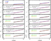 |
Fig. 1. PL relations obtained for several bands. In order, from top to bottom and left to right, we show the Gaia GBP, G, and GRP bands; Johnson-Cousins I, J, H, and K bands; VISTA J, Y, and Ks bands; and the Rubin-LSST g, r, i, z, and y bands. Different colours reflect the three different metallicities. The dashed lines correspond to the relations from RRL models (Marconi et al. 2015, 2022), while the relations from Sicignano et al. (2024) for the Gaia and VISTA bands are plotted in green and yellow. |
In Fig. 1, the relations obtained for RRL models (Marconi et al. 2015, 2022) and the empirical ones obtained from VISTA data by Sicignano et al. (2024), for the corresponding metallicities and filters, are overlapped. It seems quite evident that (i) the predicted metallicity effect on the zero point of the NIR PL relations is generally smaller for T2Cs than for RRLs, but the slopes are highly consistent; and (ii) there is an excellent agreement with results by Sicignano et al. (2024).
We note that an often-overlooked source of uncertainty arises when T2Cs stars are inadvertently classified as RRLs (or vice versa) and the corresponding PL or PLW relations are applied. Based on our results (see Figs. 8 and 9), this effect is negligible at higher metallicities, where the PL relations of the two classes nearly overlap. However, at lower metallicities, the PL zero points for T2Cs are systematically fainter, implying that using RRL PL relations would lead to brighter absolute magnitudes and consequently to underestimated distances by some tenths of magnitudes.
4.3. The PW relations
In Fig. 2, we show the obtained PW relations2 for the selected metal abundances and the labelled filter combinations. Again, theoretical RRL relations from Marconi et al. (2015) are overimposed where available, and a comparison with the empirical results by Sicignano et al. (2024) is shown for the VISTA band combinations. Similarly to what was found for RRL (see, e.g. Marconi et al. 2015, 2022, for detail), we identify optical band combinations that minimise the metallicity effect. In particular, the metallicity dependence seems to be completely negligible in the case of the PW relation involving the Rubin-LSST g and i bands and very small (but still significant given the tiny errors on coefficients), in all the other cases, making these relations very solid tools to derive individual T2C distances irrespective of uncertainties in their metal abundance. These results are in agreement with the empirical evidence provided by Groenewegen & Jurkovic (2017), which found no difference in the PL relations of T2Cs in the LMC and SMC.
5. Application to observed T2Cs
As an application of the previously derived relationships, we calculated the distances of various samples of T2Cs collected from the literature. Specifically, in the following sections, we focus on datasets belonging to the Large Magellanic Cloud (LMC), the Small Magellanic Cloud (SMC), and the MilkyWay (MW).
5.1. LMC and SMC distances
We used two samples of 149 LMC and 26 SMC T2Cs, respectively, with photometric data available from Gaia Data Release 3 (DR3; Gaia Collaboration 2023; Ripepi et al. 2023). The adopted mean values of [Fe/H] are −0.409 ± 0.076 dex and −0.78 ± 0.08 dex for the LMC and the SMC, respectively, are taken from the literature (see, e.g. Romaniello et al. 2008, 2022).
The Wesenheit magnitude in the Gaia bands, defined as WGaia = G − 1.9 ⋅ (GBP − GRP) (Ripepi et al. 2019), was taken into account. The observed Wesenheit magnitudes were obtained by applying the last equation to the mean magnitudes in the G, GBP, and GRP, retrieved from the public Gaiaarchive.
The absolute Wesenheit magnitudes in the Gaia photometric bands were obtained by applying the corresponding theoretical PWZ relation (reported in Table 3) to all the selected sources. From the difference between the absolute and observed Wesenheit magnitudes, we infer the individual distance moduli (μ0). The associated errors are evaluated by taking into account both the observational uncertainties and the rms of the adoptedrelations.
The coefficients of the PLZ and PWZ relations.
The best distance moduli for the LMC and SMC (Columns 8 and 10 of Table 3 were determined by computing the median of the distributions of the individual μ0 values derived for the T2Cs described above. The uncertainties associated with these best estimates were calculated using the robust standard deviation, defined as 1.4826 ⋅ MAD, of the corresponding distributions.
In Fig. 3, we show the distribution of μ0 values obtained by applying our theoretical PWZ relations to the selected LMC (left column) and SMC (right column) T2Cs. The results for different bands are plotted in different panels. We show that our results are slightly shorter than the value by Pietrzyński et al. (2019) and Graczyk et al. (2020), but still consistent within the errors. The worse quality of the inferred distribution in the case of the SMC is likely due to the small number of Cepheidsconsidered.
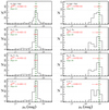 |
Fig. 3. Distributions of μ0 values obtained by applying our PWZ theoretical relations to a sample of LMC T2Cs (left panels) and SMC T2Cs (right panels). The results for different bands are plotted in different panels. From top to bottom: Gaia G, BP − RP, VISTA Ks, J − Ks, VISTA Ks, Y − Ks, and Johnson I, V − I PWZ relations. The vertical green lines represent the LMC and SMC distance ranges around the currently adopted geometric best values from Pietrzyński et al. (2019) and Graczyk et al. (2020), respectively, while the red square and the error bar indicate the median value of our distribution and its robust standard deviation (i.e. 1.4826 ⋅ MAD), respectively. |
5.2. Galactic T2Cs
We also selected a sample of 100 Galactic T2Cs from the Gaia DR3 as detailed in Sicignano et al. (2024) and repeated the analysis described above, adopting the PWZ relation in the Gaia photometric bands. Since metallicity measurements for these stars are unavailable, we tested our PWZ relations by assuming three fixed metallicity values, namely Z = 0.01, Z = 0.001, and Z = 0.0001, which correspond to those used in the computation of the pulsation models.
The individual μ0, derived by applying the PWZ relation, was converted into parallaxes to enable a direct comparison with Gaia DR3 results, including the zero-point correction provided by Lindegren et al. (2021) (L21). The resulting theoretical parallaxes (ϖteo), along with their associated uncertainties, are reported in Table 4, together with the Gaia DR3 parallaxes and L21 correction values. The comparison with Gaia astrometric results is shown in Fig. 4, for the three assumed metallicities. In each panel, the predicted theoretical parallaxes are plotted against the corrected Gaia DR3 values with a 1:1 reference line shown to make the comparison easier. The residuals, computed as ϖDR3 + L21 − ϖteo, are displayed in the three smaller panels, centred around the zero line. A statistical analysis of these residuals indicates that Gaia DR3 parallaxes, after applying the L21 correction, are systematically larger than those inferred from the pulsation models. The median differences range from a marginally significant value of 9 ± 5 μas for the most metal-poor models, up to 14.0 ± 5.4 μas for the most metal-rich ones. The uncertainties on the median values are estimated as  . Our results are consistent with recent findings in the literature, which suggest that the application of the correction proposed by Lindegren et al. (2021) tends to over-correct Gaia DR3 parallaxes, resulting in values that are systematically larger than expected. This trend has been noted in several independent studies (see, e.g. Molinaro et al. 2023, for a recent review).
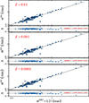 |
Fig. 4. Theoretical parallaxes of Galactic Type II Cepheids in the Gaia database, as obtained from inversion of the theoretical PWZ relation in the Gaia bands, versus Gaia astrometric values, as corrected for the Lindegren et al. (2021) offset. In each panel, we show the results obtained assuming the labelled metal abundance in the PWZ relation. The bottom plot of each panel shows the corresponding residuals computed as ϖDR3 + L21 − ϖteo. |
Adopted Galactic T2Cs.
5.3. Globular clusters
As a further test, we applied our PWZ relations in the Gaia bands to a sample of T2C host GGCs. The three large panels of Fig. 5 display our derived distance moduli (vertical axis) compared with reference values from the literature: Baumgardt & Vasiliev (2021) in the top panel and Sicignano et al. (2024) in the middle and bottom panels. In each case, the reference values are plotted on the horizontal axis. The corresponding residuals to the 1:1 relation are shown in the smaller panels below each main plot. A quick inspection suggests that Sicignano et al. (2024) distance moduli are in better agreement with the theoretical predictions than the value published by Baumgardt & Vasiliev (2021). This is not a surprise as Sicignano et al. (2024) used their derived empirical calibrations of PL and PW relations to obtain distances to these T2C-host GGCs systematically smaller by ∼0.1 mag and 0.03–0.06 mag than Baumgardt & Vasiliev (2021) when the zero points are calibrated with the distance of the LMC or Gaia parallaxes, respectively. Moreover, it is worth noting that Bhardwaj et al. (2023) also found that their derived RRL-based GGC distances are systematically smaller, by about 0.015 mag, than those provided byBaumgardt & Vasiliev (2021).
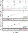 |
Fig. 5. Distance moduli derived in this work (vertical axis) for GGC T2Cs pulsators compared to those from Baumgardt & Vasiliev (2021) in the Gaia bands (top large panel), from Sicignano et al. (2024) in the Gaia bands (middle large panel), and from Sicignano et al. (2024) in the Ks, J − Ks bands (bottom large panel). The residuals are shown in the corresponding smaller panels. |
6. Conclusions
A new theoretical scenario was presented for BL Her and W Vir pulsating stars with periods up to about ten days for three selected metal abundances (Z = 0.01, 0.001, and 0.0001). The main results of this investigation are listed below
-
The obtained model predictions show that the new T2Cs theoretical instability strip is consistent with the results obtained from BL Her non-linear convective pulsation models by Di Criscienzo et al. (2007), which are slightly wider than the extrapolated RRL one (Marconi et al. 2015), but slightly narrower and/or redder than the one by Deka et al. (2024), depending on the assumed metal content.
-
The morphology of the predicted light curve varies across the instability strip with similarities to the case of RRL stars. Through the adoption of model atmospheres, we obtained theoretical light curves and pulsation amplitudes in a variety of photometric systems and for the first time in the Gaia and Rubin-LSST filters for T2C models.
-
The obtained mean magnitudes and colours have been adopted to build theoretical PL and PW relations in all the considered photometric bands and to investigate the effect of the assumed metal abundance. We find that the predicted metallicity effect on the zero point of the NIR PL relations is generally smaller for T2Cs than for RRL. Moreover, we find an excellent agreement with the results by Sicignano et al. (2024). In the case of the PW relations, similarly to what was found for RRL, we identified optical band combinations that minimise the metallicity dependence.
The application of the inferred theoretical relations to Magellanic Cloud and Galactic T2C data shows a good agreement. In particular, the LMC and SMC distance moduli, μ0, obtained as the medians of the distributions of the individual values derived for the investigated T2Cs are found to be slightly shorter than the value by Pietrzyński et al. (2019) and Graczyk et al. (2020), but still consistent within the errors. As for Galactic T2Cs, 100 targets taken from the ESA Gaia DR3 were considered. The individual distance moduli, derived by applying the PWZ relations, were converted into parallaxes to enable a direct comparison with Gaia DR3 values, including the zero-point correction provided by Lindegren et al. (2021). As a result, we found a deviation of theoretical parallaxes from Gaia results, which is consistent with published independent indications that the Lindegren et al. (2021) correction tends to overestimate Gaia parallaxes (see also Molinaro et al. 2023, for details). We finally applied our PWZ relations in the Gaia bands to a sample of T2C host GGCs. As a result, we find that Sicignano et al. (2024) distance moduli are in better agreement with the theoretical predictions than the value published by Baumgardt & Vasiliev (2021). On the basis of the obtained relations and distances, we can conclude that T2C non-linear convective pulsation models provide additional tools to constrain individual distances and stellar properties of the host old stellar populations. In the future, we plan to extend the model set to a wider range of input parameters, apply the model-fitting technique (see, e.g. Molinaro et al. 2025, and references therein), reproduce the observed multi-filter light curves available in current and future surveys, and provide a theoretical calibration of the tip of the RGB as an alternative Type II population distance indicator calibrating SNIa in the stellar route to the Hubble constant (see, e.g. Freedman 2021b, and references therein).
Data availability
Tables 1 and 4 are available at the CDS via https://cdsarc.cds.unistra.fr/viz-bin/cat/J/A+A/703/A228
Acknowledgments
We thank the anonymous referee for her/his very useful comments. We acknowledge the financial support from INAF (Large Grant MOVIE, PI: Marconi), Project PRIN MUR 2022 (code 2022ARWP9C) “Early Formation and Evolution of Bulge and HalO (EFEBHO)”, PI: M. Marconi, funded by European Union – Next Generation EU, ASI-Gaia (“Missione Gaia Partecipazione italiana al DPAC – Operazioni e Attività di Analisi dati”), the INAF GO-GTO grant 2023 “C-MetaLL – Cepheid Metallicities in the Leavitt Law” (PI: V. Ripepi) and INAF-ASTROFIT fellowship (PI: G. De Somma). This research was also supported by the International Space Science Institute (ISSI) in Bern, through ISSI International Team project SHoT: The Stellar Path to the Ho Tension in the Gaia, TESS, LSST and JWST Era. G.D.S. and T.S. thank INFN (Naples section) for support via QGSKY initiatives, with additional INFN support for Moonlight2 (G.D.S.). This research also benefited from COST Action CA21136 (CosmoVerse), addressing cosmological tensions through systematics and fundamental physics, funded by COST (European Cooperation in Science and Technology).
References
- Baade, W. 1958, AJ, 63, 207 [Google Scholar]
- Baumgardt, H., & Vasiliev, E. 2021, MNRAS, 505, 5957 [NASA ADS] [CrossRef] [Google Scholar]
- Bhardwaj, A., Braga, V. F., Minniti, D., Contreras Ramos, R., & Rejkuba, M. 2021, ASP Conf. Ser., 529, 259 [Google Scholar]
- Bhardwaj, A., Marconi, M., Rejkuba, M., et al. 2023, ApJ, 944, L51 [NASA ADS] [CrossRef] [Google Scholar]
- Bódi, A., & Kiss, L. L. 2019, ApJ, 872, 60 [CrossRef] [Google Scholar]
- Bono, G., Incerpi, R., & Marconi, M. 1996, ApJ, 467, L97 [Google Scholar]
- Bono, G., Caputo, F., Cassisi, S., Incerpi, R., & Marconi, M. 1997a, ApJ, 483, 811 [Google Scholar]
- Bono, G., Caputo, F., Castellani, V., & Marconi, M. 1997b, A&AS, 121, 327 [NASA ADS] [CrossRef] [EDP Sciences] [Google Scholar]
- Bono, G., Pietrinferni, A., Marconi, M., et al. 2016, Comm. Konkoly Obs. Hung., 105, 149 [Google Scholar]
- Bono, G., Braga, V. F., Fiorentino, G., et al. 2020, A&A, 644, A96 [NASA ADS] [CrossRef] [EDP Sciences] [Google Scholar]
- Braga, V. F., Contreras Ramos, R., Minniti, D., et al. 2019, A&A, 625, A151 [NASA ADS] [CrossRef] [EDP Sciences] [Google Scholar]
- Cassisi, S., & Salaris, M. 2011, ApJ, 728, L43 [NASA ADS] [CrossRef] [Google Scholar]
- De Somma, G., Marconi, M., Molinaro, R., et al. 2022, ApJS, 262, 25 [NASA ADS] [CrossRef] [Google Scholar]
- De Somma, G., Marconi, M., Cassisi, S., & Molinaro, R. 2024, ApJ, 977, 1 [Google Scholar]
- Deka, M., Bellinger, E. P., Kanbur, S. M., et al. 2024, MNRAS, 530, 5099 [Google Scholar]
- Di Criscienzo, M., Caputo, F., Marconi, M., & Cassisi, S. 2007, A&A, 471, 893 [NASA ADS] [CrossRef] [EDP Sciences] [Google Scholar]
- Ferguson, J. W., Alexander, D. R., Allard, F., et al. 2005, ApJ, 623, 585 [Google Scholar]
- Freedman, W. L. 2021a, ApJ, 919, 16 [NASA ADS] [CrossRef] [Google Scholar]
- Freedman, W. L. 2021b, ApJ, 919, 16 [NASA ADS] [CrossRef] [Google Scholar]
- Gaia Collaboration (Vallenari, A., et al.) 2023, A&A, 674, A1 [NASA ADS] [CrossRef] [EDP Sciences] [Google Scholar]
- Gingold, R. A. 1976, ApJ, 204, 116 [NASA ADS] [CrossRef] [Google Scholar]
- Gingold, R. A. 1985, Mem. Soc. Astron. It., 56, 169 [Google Scholar]
- Graczyk, D., Pietrzyński, G., Thompson, I. B., et al. 2020, ApJ, 904, 13 [Google Scholar]
- Groenewegen, M. A. T., & Jurkovic, M. I. 2017, A&A, 604, A29 [NASA ADS] [CrossRef] [EDP Sciences] [Google Scholar]
- Hoyt, T. J., Jang, I. S., Freedman, W. L., et al. 2025, arXiv e-prints [arXiv:2503.11769] [Google Scholar]
- Iglesias, C. A., & Rogers, F. J. 1996, ApJ, 464, 943 [NASA ADS] [CrossRef] [Google Scholar]
- Lindegren, L., Bastian, U., Biermann, M., et al. 2021, A&A, 649, A4 [EDP Sciences] [Google Scholar]
- Madore, B. F. 1982, ApJ, 253, 575 [NASA ADS] [CrossRef] [Google Scholar]
- Manick, R., Van Winckel, H., Kamath, D., et al. 2018, A&A, 618, 21 [Google Scholar]
- Marconi, M., & Di Criscienzo, M. 2007, A&A, 467, 223 [EDP Sciences] [Google Scholar]
- Marconi, M., Coppola, G., Bono, G., et al. 2015, ApJ, 808, 50 [Google Scholar]
- Marconi, M., Bono, G., Pietrinferni, A., et al. 2018, ApJ, 864, L13 [Google Scholar]
- Marconi, M., Molinaro, R., Dall’Ora, M., et al. 2022, ApJ, 934, 29 [NASA ADS] [CrossRef] [Google Scholar]
- Matsunaga, N., Fukushi, H., Nakada, Y., et al. 2006, MNRAS, 370, 1979 [Google Scholar]
- Matsunaga, N., Feast, M. W., Kawadu, T., et al. 2013, MNRAS, 429, 385 [CrossRef] [Google Scholar]
- Molinaro, R., Ripepi, V., Marconi, M., et al. 2023, MNRAS, 520, 4154 [NASA ADS] [CrossRef] [Google Scholar]
- Molinaro, R., Marconi, M., De Somma, G., et al. 2025, A&A, 700, A212 [NASA ADS] [CrossRef] [EDP Sciences] [Google Scholar]
- Ngeow, C.-C., Bhardwaj, A., Henderson, J.-Y., et al. 2022, AJ, 164, 154 [NASA ADS] [CrossRef] [Google Scholar]
- Origlia, L., Ferraro, F. R., Fabbri, S., et al. 2014, A&A, 564, A136 [NASA ADS] [CrossRef] [EDP Sciences] [Google Scholar]
- Pietrzyński, G., Graczyk, D., Gallenne, A., et al. 2019, Nature, 567, 200 [Google Scholar]
- Planck Collaboration VI. 2020, A&A, 641, A6 [NASA ADS] [CrossRef] [EDP Sciences] [Google Scholar]
- Riess, A. G., Yuan, W., Macri, L. M., et al. 2022, ApJ, 934, L7 [NASA ADS] [CrossRef] [Google Scholar]
- Ripepi, V., Moretti, M. I., Marconi, M., et al. 2015, MNRAS, 446, 3034 [NASA ADS] [CrossRef] [Google Scholar]
- Ripepi, V., Molinaro, R., Musella, I., et al. 2019, A&A, 625, A14 [NASA ADS] [CrossRef] [EDP Sciences] [Google Scholar]
- Ripepi, V., Clementini, G., Molinaro, R., et al. 2023, A&A, 674, A17 [NASA ADS] [CrossRef] [EDP Sciences] [Google Scholar]
- Romaniello, M., Primas, F., Mottini, M., et al. 2008, A&A, 488, 731 [NASA ADS] [CrossRef] [EDP Sciences] [Google Scholar]
- Romaniello, M., Riess, A., Mancino, S., et al. 2022, A&A, 658, A29 [NASA ADS] [CrossRef] [EDP Sciences] [Google Scholar]
- Scolnic, D., Riess, A. G., Wu, J., et al. 2023, ApJ, 954, L31 [NASA ADS] [CrossRef] [Google Scholar]
- Sicignano, T., Ripepi, V., Marconi, M., et al. 2024, A&A, 685, A41 [NASA ADS] [CrossRef] [EDP Sciences] [Google Scholar]
- Soszyński, I., Udalski, A., Szymański, M. K., et al. 2008, Acta Astron., 58, 293 [NASA ADS] [Google Scholar]
- Soszyński, I., Udalski, A., Pietrukowicz, P., et al. 2011, Acta Astron., 61, 285 [NASA ADS] [Google Scholar]
- Soszyński, I., Udalski, A., Szymański, M. K., et al. 2017, Acta Astron., 67, 297 [NASA ADS] [Google Scholar]
- Soszyński, I., Udalski, A., Szymański, M. K., et al. 2018, Acta Astron., 68, 89 [NASA ADS] [Google Scholar]
- Van Albada, T., & Baker, N. 1971, ApJ, 169, 311 [NASA ADS] [CrossRef] [Google Scholar]
- Verde, L., Treu, T., & Riess, A. G. 2019, Nat. Astron., 3, 891 [Google Scholar]
The coefficient of determination, R2, quantifies the proportion of variance in the observed data explained by the model. An R2 value close to 1 indicates a good fit, while values near 0 imply a poor explanatory power.
Wesenheit magnitudes, introduced by Madore (1982), provide reddening-free magnitudes once we assume to know the extinction law. They are defined as WX1, X2 − X3 = X1 − ξ12; 3 ⋅ (X2 − X3), where Xi indicates the generic band and the coefficient ξ12, 3 coincides with the total-to-selective absorption.
Appendix A: Figures that are not shown in the text
In Figure A.1 we show a subset of the stellar evolutionary tracks presented by Bono et al. (2020) (see their Fig. 5), with a wide range of stellar masses (M/M⊙ ≈ 0.50-0.90) and three different initial metal abundances, namely Z = 0.01 (top panel), Z = 0.001 (middle panel), Z = 0.0001 (bottom panel).
In Fig. A.2 we show an example of the produced atlas of bolometric light curves, whereas Figure A.3 shows the radial velocity curves for the same models.
In Fig. A.4 and A.5 we show the same curves already displayed in Fig. A.2 but in the Gaia and Rubin-LSST bands, respectively.
In Fig. A.6 we show the predicted period-amplitude diagram in the three Gaia bands for all the computed models and the labelled metal abundances. The same diagram but for the Rubin-LSST bands is shown in Fig. .
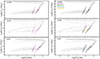 |
Fig. A.1. Left: the predicted F-mode instability strips (solid lines) for the three labelled metallicities over-imposed to the evolutionary tracks from Bono et al. (2020). Right: the same but compared with the extrapolated RRL instability strip, as predicted by Marconi et al. (2015) and shown in Bono et al. (2020) (green lines), for each selected metallicity, together with the recently derived BL Her instability strip by Deka et al. (2024) (blue lines) and the previously computed boundaries by Di Criscienzo et al. (2007) (orange lines). |
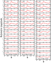 |
Fig. A.2. Example of predicted bolometric light curves with decreasing effective temperature and the highest computed stellar mass (see labels) for each metallicity Z = 0.0001 (left panel), Z = 0.001 (middle panel) and Z = 0.01 (right panel). |
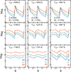 |
Fig. A.4. An example of predicted GBP (red), G (green) and GRP (blue) light curves for Z = 0.0001 (left panel), Z = 0.001 (middle panel) and Z = 0.01 (right panel). The three vertical panels correspond to different values of the model stellar mass and metallicity (see labels). Three values of the effective temperature are considered and labelled in each panel. |
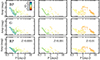 |
Fig. A.6. Predicted period-amplitude diagrams for the Gaia bands (top:GBP, middle: G, bottom: GRP) for all the computed models and the labelled metal abundances (left: Z = 0.0001, center: Z = 0.001, right: Z= 0.01), colour-coded by the assumed stellar mass. |
All Tables
All Figures
|
Fig. 1. PL relations obtained for several bands. In order, from top to bottom and left to right, we show the Gaia GBP, G, and GRP bands; Johnson-Cousins I, J, H, and K bands; VISTA J, Y, and Ks bands; and the Rubin-LSST g, r, i, z, and y bands. Different colours reflect the three different metallicities. The dashed lines correspond to the relations from RRL models (Marconi et al. 2015, 2022), while the relations from Sicignano et al. (2024) for the Gaia and VISTA bands are plotted in green and yellow. |
| In the text | |
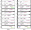 |
Fig. 2. PW relation calculated in this work. Colours and line style are the same as in Fig. 1. |
| In the text | |
|
Fig. 3. Distributions of μ0 values obtained by applying our PWZ theoretical relations to a sample of LMC T2Cs (left panels) and SMC T2Cs (right panels). The results for different bands are plotted in different panels. From top to bottom: Gaia G, BP − RP, VISTA Ks, J − Ks, VISTA Ks, Y − Ks, and Johnson I, V − I PWZ relations. The vertical green lines represent the LMC and SMC distance ranges around the currently adopted geometric best values from Pietrzyński et al. (2019) and Graczyk et al. (2020), respectively, while the red square and the error bar indicate the median value of our distribution and its robust standard deviation (i.e. 1.4826 ⋅ MAD), respectively. |
| In the text | |
|
Fig. 4. Theoretical parallaxes of Galactic Type II Cepheids in the Gaia database, as obtained from inversion of the theoretical PWZ relation in the Gaia bands, versus Gaia astrometric values, as corrected for the Lindegren et al. (2021) offset. In each panel, we show the results obtained assuming the labelled metal abundance in the PWZ relation. The bottom plot of each panel shows the corresponding residuals computed as ϖDR3 + L21 − ϖteo. |
| In the text | |
|
Fig. 5. Distance moduli derived in this work (vertical axis) for GGC T2Cs pulsators compared to those from Baumgardt & Vasiliev (2021) in the Gaia bands (top large panel), from Sicignano et al. (2024) in the Gaia bands (middle large panel), and from Sicignano et al. (2024) in the Ks, J − Ks bands (bottom large panel). The residuals are shown in the corresponding smaller panels. |
| In the text | |
|
Fig. A.1. Left: the predicted F-mode instability strips (solid lines) for the three labelled metallicities over-imposed to the evolutionary tracks from Bono et al. (2020). Right: the same but compared with the extrapolated RRL instability strip, as predicted by Marconi et al. (2015) and shown in Bono et al. (2020) (green lines), for each selected metallicity, together with the recently derived BL Her instability strip by Deka et al. (2024) (blue lines) and the previously computed boundaries by Di Criscienzo et al. (2007) (orange lines). |
| In the text | |
|
Fig. A.2. Example of predicted bolometric light curves with decreasing effective temperature and the highest computed stellar mass (see labels) for each metallicity Z = 0.0001 (left panel), Z = 0.001 (middle panel) and Z = 0.01 (right panel). |
| In the text | |
 |
Fig. A.3. Same as Fig. A.2 but for radial velocity curves. |
| In the text | |
|
Fig. A.4. An example of predicted GBP (red), G (green) and GRP (blue) light curves for Z = 0.0001 (left panel), Z = 0.001 (middle panel) and Z = 0.01 (right panel). The three vertical panels correspond to different values of the model stellar mass and metallicity (see labels). Three values of the effective temperature are considered and labelled in each panel. |
| In the text | |
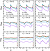 |
Fig. A.5. The same as Fig. A.5 but for the Rubin-LSST filters. |
| In the text | |
|
Fig. A.6. Predicted period-amplitude diagrams for the Gaia bands (top:GBP, middle: G, bottom: GRP) for all the computed models and the labelled metal abundances (left: Z = 0.0001, center: Z = 0.001, right: Z= 0.01), colour-coded by the assumed stellar mass. |
| In the text | |
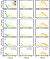 |
Fig. A.7. Same as Fig. A.6 but for the 6 Rubin-LSST bands labelled in the first column of each row. |
| In the text | |
Current usage metrics show cumulative count of Article Views (full-text article views including HTML views, PDF and ePub downloads, according to the available data) and Abstracts Views on Vision4Press platform.
Data correspond to usage on the plateform after 2015. The current usage metrics is available 48-96 hours after online publication and is updated daily on week days.
Initial download of the metrics may take a while.