| Issue |
A&A
Volume 703, November 2025
|
|
|---|---|---|
| Article Number | A147 | |
| Number of page(s) | 13 | |
| Section | Interstellar and circumstellar matter | |
| DOI | https://doi.org/10.1051/0004-6361/202556498 | |
| Published online | 13 November 2025 | |
A high geometric albedo and small size for the Haumea cluster member (24835) 1995 SM55 determined from a stellar occultation and photometric observations
1
Instituto de Astrofisica de Andalucía, IAA-CSIC,
Glorieta de la Astronomía s/n,
18008
Granada,
Spain
2
LTE, Observatoire de Paris, Université PSL, Sorbonne Université, Université de Lille,
LNE, CNRS 61 Avenue de l’Observatoire,
75014
Paris,
France
3
Florida Space Institute (FSI) – University of Central Florida (UCF),
Partnership I, Research Parkway,
32826
Orlando,
USA
4
Federal University of Technology - Paraná (PPGFA/UTFPR-Curitiba),
Av. Sete de Setembro,
3165
Curitiba –
PR,
Brazil
5
Laboratório Interinstitucional de e-Astronomia - LIneA,
Av. Pastor Martin Luther King Jr 126,
20765-000
Rio de Janeiro,
RJ,
Brazil
6
LIRA, CNRS UMR8254, Observatoire de Paris, Université PSL, Sorbonne Université, Université Paris Cité, CY Cergy Paris Université,
92190
Meudon,
France
7
Federal University of Rio de Janeiro – Observatory of Valongo,
Rio de Janeiro,
Brazil
8
Deutsches Zentrum für Astrophysik (DZA),
Postplatz 1,
02826
Görlitz,
Germany
9
Institut Polytechnique des Sciences Avancées IPSA,
63 boulevard de Brandebourg,
94200
Ivry-sur-Seine,
France
10
Türkiye National Observatories, TUG,
07070
Antalya,
Türkiye
11
The Scientific and Technological Research Council of Türkiye (TÜBİTAK),
06680
Ankara,
Türkiye
12
School of Physics & Astronomy and the Wise Observatory, Tel-Aviv University,
Tel-Aviv
6997801,
Israel
13
Astronomical Observatory Institute, Faculty of Physics and Astronomy, Adam Mickiewicz University,
Słoneczna 36,
60-286
Poznań,
Poland
14
Astronomical Observatory, Cluj-Napoca Branch, Astronomical Institute of the Romanian Academy,
Cluj-Napoca,
Romania
15
Astronomical Institute of the Romanian Academy,
5 Cutitul de Argint Street,
040557
Bucharest,
Romania
16
Université de Liège, Space Sciences, Technologies and Astrophysics Research Institute (STAR),
COMETA,
Belgium
17
Royal Observatory of Belgium,
Avenue Circulaire 3,
1180
Uccle,
Belgium
18
naXys, Department of Mathematics, University of Namur,
Rue de Bruxelles 61,
Namur
5000,
Belgium
19
Observatório Nacional/MCTI,
R. General José Cristino 77,
CEP 20921-400
Rio de Janeiro –
RJ,
Brazil
20
UNESP-São Paulo State University, Grupo de Dinâmica Orbital e Planetologia,
CEP 12516-410,
Guaratinguetá,
SP,
Brazil
21
University Observatory Munich, Faculty of Physics, Ludwig-Maximilians-Universität München,
Scheinerstr. 1,
81679
Munich,
Germany
22
National Research Institute of Astronomy and Geophysics (NRIAG),
11421
Helwan,
Cairo,
Egypt
23
Črni Vrh Observatory,
Predgriže 29A,
5274
Črni Vrh nad Idrijo,
Slovenia
24
University of Ljubljana, Faculty of Mathematics and Physics,
Jadranska 19,
1000
Ljubljana,
Slovenia
25
Dark Sky Slovenia,
Savlje 89,
1000
Ljubljana,
Slovenia
26
Société Astronomique de Liège,
Belgium
27
Department of Physical Geography and Geoecology, Faculty of Science, Charles University,
Prague,
Czech Republic
28
Department of Spatial Ecology, Landscape Research Institute,
Pruhonice,
Czech Republic
29
TÜRKSAT Satellite Communication, Cable TV and Operation Inc.,
Gölbaşı,
Ankara,
Türkiye
30
Department of Astronomy and Space Sciences, Faculty of Science, Istanbul University,
34116
Istanbul,
Türkiye
31
Istanbul University Observatory Research and Application Centre,
34116
Istanbul,
Türkiye
32
ISTEK Belde Observatory,
Istanbul,
Türkiye
33
Konkoly Observatory, HUN-REN Research Centre for Astronomy and Earth Sciences,
Konkoly Thege 15-17,
1121
Budapest,
Hungary
34
CSFK, MTA Centre of Excellence, Budapest,
Konkoly Thege 15–17,
Budapest
1121,
Hungary
35
ELTE Eötvös Loránd University, Institute of Physics and Astronomy,
Budapest,
Hungary
36
Czech Astronomical Society, IOTA-ES
37
Institute of Space Science – INFLPR Subsidiary,
Măgurele,
Romania
38
Section of Astrophysics, Astronomy and Mechanics, Department of Physics, National and Kapodistrian University of Athens,
15784
Zografos,
Athens,
Greece
39
Starhoper Observatory,
Romania
40
Dipartimento di Fisica e Astronomia “Galileo Galilei” – Università degli Studi di Padova,
Vicolo dell’Osservatorio 3,
35122
Padova,
Italy
41
INAF – Osservatorio Astronomico di Padova,
vicolo dell’Osservatorio 5,
35122
Padova,
Italy
42
Observatory Rokycany and Pilsen,
Czech Republic
43
Department of Physics, Adiyaman University,
Adiyaman
02040,
Türkiye
44
Department of Physics, The George Washington University,
Washington,
DC 20052,
USA
45
University of National Education Commission,
Krakow,
Poland
46
Fondazione GAL Hassin – Centro Internazionale per le Scienze Astronomiche,
Via della Fontana Mitri,
90010
Isnello,
Italy
47
Montarrenti Observatory,
Str. di Montarrenti, 2,
53018
Sovicille,
Siena,
Italy
48
Astronomical Observatory, Department of Physical Sciences, Earth and Environment, University of Siena,
Via Roma 56,
53100
Siena,
Italy
49
Department of Mechatronics Engineering, Faculty of Engineering and Natural Sciences, Istanbul Health and Technology University,
34445
Istanbul,
Türkiye
50
Space Science and Solar Energy Research and Application Center (UZAYMER), University of Çukurova,
Adana
01330,
Türkiye
51
Yüregir Science Center
Adana
01260,
Türkiye
52
Mesopotamia Astronomy Association,
Batman
72040,
Türkiye
53
International Occultation Timing Association/European Section,
Am Brombeerhag 13,
30459
Hannover,
Germany
54
UAI – Unione Astrofili Italiani, GAMP – Gruppo Astrofili Montagna
Pistoiese,
Italy
55
Department of Astronomy, Faculty of Mathematics, University of Belgrade,
Serbia
56
Astronomical Observatory of Belgrade,
Serbia
57
Vasile Lucaciu National College,
Baia Mare,
Romania
58
Eskişehir Technical University, Astrophysics Education and Research Unit,
Eskişehir,
Türkiye
59
Astronomical Institute of the Czech Academy of Sciences,
Fričova 298,
251 65
Ondřejov,
Czech Republic
60
Associazione Astronomica Antares APS,
Italy
61
Osservatorio Astronomico di Monte Agliale,
Via Cune Motrone,
55023
Borgo a Mozzano,
Italy
62
ELTE Eötvös Loránd University, Gothard Astrophysical Observatory,
9700
Szombathely,
Szent I. h. u 112,
Hungary
63
Astronomical Institute, Slovak Academy of Sciences,
059 60
Tatranská Lomnica,
Slovakia
64
Valasské Meziříčí Observatory,
Czech Republic
65
Bavarian Public Observatory,
Munich,
Germany
66
Astroclub Radebeul e.V.,
Radebeul,
Germany
67
Harpoint Observatory,
Harpoint,
Austria
68
EUR ING,
Hviezdoslavova 1971,
022 01
Cadca,
Slovakia
69
Ondokuz Mayis University Observatory,
Kurupelit Campus,
55139
Atakum, Samsun,
Türkiye
★ Corresponding author: This email address is being protected from spambots. You need JavaScript enabled to view it.
Received:
18
July
2025
Accepted:
16
September
2025
Abstract
Context. Trans-Neptunian objects (TNOs) are thought to be some of the most ancient and primitive bodies in our Solar System. Understanding their basic physical properties is crucial to unraveling their origin and the evolution of the outer Solar System beyond Neptune. Stellar occultations are a highly effective and sensitive method of studying these distant and faint objects, allowing us to gather essential information about their physical characteristics. (24835) 1995 SM55 is one of the few members of the Haumea orbital cluster and, therefore, is an especially relevant body to study within the TNO population.
Aims. The main objectives of the present work are to determine the projected size, absolute magnitude, and geometric albedo of 1995 SM55 and to analyze the results compared to Haumea.
Methods. We predicted a stellar occultation by this TNO for February, 25, 2024, carried out a specific campaign to observe the occultation, and derived the projected size and shape from the occultation observations using an elliptical fit to the occultation chords. We also analyzed a large set of photometric observations of (24835) 1995 SM55 to obtain the absolute magnitude and the rotational period. Finally, we combined these results to derive the geometric albedo of this TNO.
Results. The occultation was successfully detected from seven instruments located at five different sites; 33 other sites reported negative detections. Using an elliptical fit to the occultation chords, we determined the size and shape of the limb of (24835) 1995 SM55 during the occultation: an ellipse with semi-axes (104.3 ± 0.4) × (83.5 ± 0.5) km. The area-equivalent diameter (Deq,A) for this ellipse is 186.7 ± 1.8 km. This is consistent with the upper limit of 250 km estimated from Herschel Observatory thermal data. From our photometric observations, we derived an absolute magnitude (HV) of 4.55 ± 0.03, a phase slope parameter of 0.04 ± 0.02 mag/deg, and a V − R value of 0.37 ± 0.05. The rotational variability has a maximum peak-to-valley amplitude (∆m) of 0.05 mag, but we could not derive an unambiguous rotational period. Combining the projected size from the occultation with the absolute photometry, we obtained a geometric albedo in the V band (pV) of 0.80 ± 0.04 for 1995 SM55. This value is remarkably high for a TNO and somewhat higher than that of Haumea, but consistent with the concept that 1995 SM55 is a member of the orbital cluster of Haumea.
Key words: occultations / Kuiper belt: general / Kuiper belt objects: individual: (24835) 1995 SM55
Publisher note: The author's name "S. Fiek" was incorrect. It has been corrected to "S. Fişek" on 18 November 2025.
© The Authors 2025
 Open Access article, published by EDP Sciences, under the terms of the Creative Commons Attribution License (https://creativecommons.org/licenses/by/4.0), which permits unrestricted use, distribution, and reproduction in any medium, provided the original work is properly cited.
This article is published in open access under the Subscribe to Open model. This email address is being protected from spambots. You need JavaScript enabled to view it. to support open access publication.
1 Introduction
Trans-Neptunian objects (TNOs), defined as celestial bodies with a semimajor axis exceeding Neptune’s, along with Centaurs (thought to be in a transitional phase between TNOs and Jupiter-family comets; e.g., Horner et al. 2004; Sarid et al. 2019), are considered some of the least altered objects since the Solar System’s genesis. Their preserved primordial characteristics and materials offer a unique window into the early stages of Solar System formation and evolution. Consequently, investigating their physical and dynamical attributes is a potent method for learning more about these formative periods. Currently, over 5000 TNOs and Centaurs have been identified, though their total population is believed to surpass that of asteroids in the main asteroid belt.
Due to their considerable distance from the Sun, TNOs present a challenge for optical observation, as the brightness of a Solar System body diminishes with the fourth power of its heliocentric distance. The vast majority of these objects typically exhibit magnitudes fainter than 20 in visible light. Furthermore, with average surface temperatures of approximately 30–40 K, their thermal emission peaks in the far-IR, a spectral region significantly attenuated by Earth’s atmosphere. Aside from a few exceptionally large TNOs, determining radiometric sizes for this population generally requires observations with ALMA or space telescopes, similar to the approach taken by the ESA Herschel mission’s “TNOs are Cool” open time key program (e.g., Müller et al. 2009; Lellouch et al. 2013; Farkas-Takács et al. 2020, and references therein) for over 120 TNOs and Centaurs. That said, stellar occultations provide an alternative means to derive sizes and albedos, potentially with greater precision than from thermal data.
The use of stellar occultations is an effective method for directly measuring the sizes and shapes of Solar System bodies, often achieving sub-kilometer accuracies (depending on timing and photometric precision). It also enables their immediate surroundings to be probed for features like rings (Braga-Ribas et al. 2014; Ortiz et al. 2015, 2017; Morgado et al. 2023) and offers the potential to identify binary systems (Leiva et al. 2020) and discover moons (e.g., Gault et al. 2022). This method can furthermore be used to detect or constrain the presence of atmospheres down to nano-bar pressure levels (e.g., Hubbard et al. 1988; Sicardy et al. 2003; Oliveira et al. 2022).
Moreover, multi-chord occultation observations yield angular positional measurements of the occulting object with sub-milliarcsecond accuracy, leveraging the high precision of the Gaia reference system (Rommel et al. 2020; Ferreira et al. 2022; Kaminski et al. 2023). This can be used to significantly refine orbital parameters and, consequently, improve predictions for the shadow path of future occultations. Unlike occultations by asteroids, forecasting and successfully observing stellar occultations by TNOs is typically very demanding (Ortiz et al. 2020), primarily due to the minute angular sizes of TNOs coupled with often substantial ephemeris uncertainties.
Trans-Neptunian object (24835) 1995 SM55 was discovered by the 0.9 m Spacewatch telescope at Steward Observatory (Kitt Peak, Arizona)on September 19, 1995 (MPEC 1999-L24). This object holds particular significance within the TNO population as one of the few recognized members of a cluster of bodies with orbital characteristics highly similar to those of the dwarf planet Haumea. While these Haumea-like bodies have been proposed as a typical collisional family resulting from a disruptive impact (Brown et al. 2007), they do not fully satisfy several criteria for collisional families (Schlichting & Sari 2009). Instead, they more closely resemble asteroid clusters (Ortiz et al. 2019) or mini-families, which are now understood to form from rotational ejections following a nondisruptive collision (Pravec et al. 2018). A similar formation mechanism was suggested for the Haumea system by Ortiz et al. (2012), who analyzed various rotational fission scenarios. For these reasons, we refer to the set of bodies with orbits related to that of Haumea as a cluster rather than a family. Given that the members would have been formed from the crust of the progenitor, their surfaces should also have similar characteristics. Indeed, the color and spectrum of 1995 SM55 are highly consistent with those of other cluster members, though its geometric albedo remained an unknown, particularly with regards to whether it aligns with Haumea’s.
This body, as part of the “TNOs are Cool” project’s target list, was observed by the Herschel Space Observatory, but no signal was detected. Consequently, only an upper limit on its size and a lower limit on its albedo could be determined (Vilenius et al. 2018), and this lower limit – 0.36 – was already unusually high for a TNO. This was also the case for other known members of the Haumea orbital cluster (see Müller et al. 2020 for a review). Therefore, 1995 SM55 presented an excellent opportunity for study via the occultation technique to precisely ascertain its size, shape, and geometric albedo.
An extensive observational campaign, involving 50 telescopes, was organized to observe a stellar occultation by 1995 SM55 on February 25, 2024. This effort was prompted by an astrometric update shortly before the event, which indicated a high probability of detection. Given that the occulted star was relatively bright (12.4 mag in the Gaia G filter), making it accessible to numerous instruments, the likelihood of success was considerable. Ultimately, seven positive detections were secured from five different observatories, while 33 sites reported negative results.
In this paper we present the observations of the stellar occultation by 1995 SM55 and the primary results derived from this event (Sect. 2). We also incorporate photometric measurements from observations of this target, accumulated over more than a decade from various telescope facilities, to estimate its absolute magnitude, phase slope, and rotational light curve. Finally, we combine all these findings to provide an accurate determination of 1995 SM55’s geometric albedo (Sect. 4). We conclude with an analysis and discussion of these results.
2 The February 25, 2024, occultation
2.1 Prediction
Within the framework of the Lucky Star collaboration1, we generated a prediction for a stellar occultation of a G = 12.3 mag star, scheduled for February 25, 2024. This prediction was computed using the Gaia Data Release 3 (DR3) star catalog in conjunction with the NIMA ephemerides (Desmars et al. 2015). Table 1 summarizes the pertinent occultation parameters and critical details of the occulted star. The specific prediction data presented in Table 1 were sourced from the nominal NIMA (version 9) prediction2. Some time prior to the occultation date, the prediction was updated and refined through the acquisition of high-precision astrometry. This astrometric data were obtained using the 2 m Liverpool Telescope (LT) at the Roque de Los Muchachos Observatory (ORM) on La Palma, Spain, as well as the 1.5 m telescope at Sierra Nevada Observatory (Granada, Spain), the 1.2 m telescope at Calar Alto Observatory (Almería, Spain) and the T120 at PHP (Observatoire de Haute Provence, France). This updated information resulted in a eastward shift of the shadow path, directing it into a region with favorable observational prospects (Fig. 1).
2.2 Observations
During the event, meteorological conditions were unfavorable across significant portions of the occultation path. Nevertheless, we successfully obtained seven positive detections from five distinct observatories located in Poland, Romania, Turkey, and Israel. Additionally, we recorded instances of near misses both to the south and north of the object (as depicted in Fig. 1, and detailed in Table A.1.
The Occultation Portal (Kilic et al. 2022)3 was utilized for observation reporting and data archival. Synthetic aperture photometry was performed on the reduced images to derive the occultation light curves. The seven positive detections are presented in Fig. 2.
The star’s apparent diameter was determined to be 0.0228 mas (in the V band) and 0.0225 mas (in the B band), calculated using formulas published by Kervella et al. (2004). This corresponds to a projected distance of 0.6 km at 1995 SM55’s location, or a duration of 0.06 s for the shadow’s velocity of 10.42 km/s. The Fresnel scale,  , is calculated to be 1.32 km or 0.134 s for a wavelength band of λ = 700 ± 300 nm. Given that all positive detections were recorded with exposure times of ≥2 s, any effects stemming from diffraction or the apparent stellar diameter are negligible, with the specific exception of the Chalin light curve, for which these effects were considered during the determination of ingress and egress times.
The ingress (disappearance) and egress (reappearance) times were extracted from the fitted occultation light curves and subsequently converted into chords on the sky plane. For modeling the light curves and fitting the profile, we employed the SORA Python package (Gomes-Júnior et al. 2022). This package also provides capabilities for extracting ingress and egress times using models that account for stellar diameter and diffraction effects where necessary. The extracted timings are listed in Table 2.
Occultation circumstances and target star parameters for (24835) 1995 SM55 on February 25, 2024.
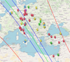 |
Fig. 1 Map of the ground track from our refined prediction, which incorporated astrometry acquired at the 1.5 m Sierra Nevada telescope, the 1.2 m Calar Alto telescope, and the 2 m Liverpool telescope. The blue lines mark the boundaries of the body’s shadow, calculated assuming a spherical shape with a diameter (D) of 398 km. The central path is indicated by a green line. Red lines illustrate the 3-sigma uncertainties associated with the prediction. The map also shows the observation sites: green markers denote positive detections, red negative detections (i.e., “misses”), blue planned but unexecuted observations, yellow locations with adverse weather, and purple technical problems. Map credit: OpenStreetMap. |
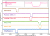 |
Fig. 2 Occultation light curves from the various instruments that successfully registered the event. The light curves (flux versus time) are normalized to one, with an arbitrary offset applied for enhanced clarity. Dots represent the observational data, while the lines correspond to the model as described in Sect. 2. The Chalin light curve (pink) is enlarged the inset. |
2.3 Elliptical fit to the projected shape
Assuming the object’s form is either spheroidal or a triaxial ellipsoid, its projection onto the sky plane can be accurately represented as an ellipse. Consequently, we fitted an ellipse to the extremities of the chords, which were derived from the disappearance and appearance times as outlined in Sect. 2.2. We also incorporated data from near misses of the occultation as additional constraints (Fig. 3). The five parameters of the fitted ellipse are: the center of the ellipse (f, 𝑔) with respect to the fundamental plane’s origin, which is defined by the geocentric star position at the event time and the TNO’s ephemeris; the apparent semimajor axis a′; the apparent oblateness ϵ′ = (a′ − b′)/a′; and the position angle of the ellipse φ′4. The prime (′) notation is used to denote that these parameters correspond to the object’s projected (“apparent”) profile ellipse, distinguishing them from the axes of a physical body (a triaxial ellipsoid with semi-axes a, b, c). These parameters were estimated using a Levenberg-Marquardt optimization algorithm. The goodness of the fit was assessed using the χ2 per degree of freedom (pdf) value, defined as  , where N = 14 represents the number of data points and M = 5 is the number of adjustable parameters. An ideal value for this metric is close to one. Our fit yielded
  . The 1σ-uncertainties in the retrieved parameters were determined via a grid search in the parameter space, specifically by varying one parameter from its nominal solution while keeping the other parameters constant. Acceptable values were those that produced a χ2 within the range
  to
to  . The results for our best-fitting instantaneous limb ellipse are summarized in Table 3.
It should be noted that the chord from Chalin is basically grazing the body as shown in the elliptical fit. In those situations, topographic relief can cause features in the observed occultation light curves. This could be the case here. Hence, we analyzed the curve in some detail here. In Fig. 4, we show a zoomed version of the light curve where strong Fresnel diffraction effects are observed both at ingress and egress together with a gradual drop to minimum flux and gradual rise to the normal stellar flux. To fit those features, the velocity of the body with respect to the star must be lower than the 10.41 km/s nominal velocity, but this difference can be explained by the inclination between the limb and the occultation path, and the presence of some topography may be playing a small role. There is some structure at the bottom of the light curve but the oscillations are at the noise level and accurate measurements of the height and depth of the potential elevations and depressions cannot be accurately derived. A fit with no topography and a velocity of 4.07 ± 0.82 km/s is shown in Fig. 4 to illustrate this point.
Ingress and egress times obtained for the February 25, 2024, occultation.
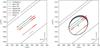 |
Fig. 3 Left: positive chords obtained from the sites indicated in the legend. Red segments illustrate the 1σ uncertainties originating from errors in ingress and egress times. Note that the large uncertainties come from the fact that the detector was at readout when the star reappeared. Continuous gray lines denote locations where negative data were obtained. Right: elliptical fit to the chords from the February 25, 2024, occultation. This fit characterizes the limb of 1995 SM55 as projected onto the sky plane, defined by the (f, g) axes with origin on the NIMA v10 ephemeris, at the moment of the occultation. The two chords obtained using the T100 and RTT150 telescopes at the Türkiye National Observatories are graphically indistinguishable in these plots, as are those from the two telescopes at Wise Observatory. The gray shaded area represents the 3σ-uncertainty region of the derived ellipse. |
Elliptical fit to the occultation profile.
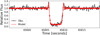 |
Fig. 4 Grazing light curve at Chalin (black dots) together with a model fit (red line) as described in the text. The light curve (flux versus time) clearly shows diffraction spikes at both disappearance and reappearance. |
3 Photometry
To comprehensively interpret occultation outcomes concerning an occulting body’s 3D shape and size, reliance on a single occultation (which captures a specific rotational phase) is insufficient. Instead, additional stellar occultations at varying rotational phases, i.e., epochs are ideal. Alternatively, leveraging rotational light curves can impose valuable constraints on a TNO’s physical model when combined with occultation data, provided that brightness variations are primarily shape-driven rather than albedo-driven. For these reasons, we analyzed existing images of 1995 SM55 from our long-term TNO photometry program and conducted new observations to ascertain its rotational light curve.
Our dataset comprises 649 observations acquired with the 1.5 m telescope at Sierra Nevada Observatory (Spain), the 1.2 m telescope at Calar Alto Observatory (Spain), and the 2 m Liver-pool Telescope on La Palma (as discussed in Sect. 2.1). Observations with the Liverpool Telescope utilized the IO:O instrument and a Sloan r′ filter. At the 1.5 m Sierra Nevada telescope, an Andor iKon-L CCD camera (model DZ936N-BEX2-DD)5 was used, sometimes without filters and other times with Johnson R and V filters. The 1.2 m Calar Alto telescope employed the DLR-MKIII instrument6, similarly observing without filters or with Johnson R and V filters. Exposure times typically ranged from 300 to 500 seconds. Image reduction and photometric analysis were performed consistently across data from all three telescopes, applying standard bias and flat-field corrections to the raw science images. The observations span from September 2012 to March 2024.
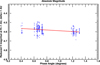 |
Fig. 5 Reduced magnitude, mV (1, 1, α), plotted against the phase angle, α. A total of 649 observations, obtained with the 2 m Liverpool telescope, the 1.5 m telescope at Sierra Nevada Observatory, and the 1.2 m telescope at Calar Alto Observatory, were analyzed. This plot was constructed after applying a sigma-clip rejection for outliers and selecting images with a signal-to-noise ratio greater than 30. |
3.1 Absolute magnitude
From the processed CCD images, we determined magnitudes in the R band and V band using our own algorithms. These algorithms utilize Gaia DR3 field stars to derive photometric transformation equations that incorporate color information (Morales et al. 2022). For 1995 SM55’s color, uncorrected for solar color, we adopted a V − R value of 0.37 ± 0.05, obtained from closely spaced V and R observations at the Calar Alto 1.2 m telescope. This value aligns well with the known color for most members of the Haumea cluster. The R-filter dataset was the most extensive. By performing a linear regression of the reduced R magnitude (representing the apparent magnitude the TNO would have at 1 au from both the Sun and Earth) against the phase angle (α), we determined the absolute magnitude, mR(1, 1, 0) (HR ), and the phase slope, β (Fig. 5). From this fitted trend line, we derived an absolute magnitude HR = 4.18 ± 0.01 and a slope parameter β = 0.04 ± 0.02 mag/°. Our observations encompassed the phase angle range α = [0.36°, 1.54°]. The observed scatter around the trend line may suggest a rotational modulation, albeit with a potential amplitude below 0.1 mag.
3.2 Rotational light curve
After removing the linear phase trend from the photometry (using the O-C residuals of the linear fit discussed in Sect. 3.1), and correcting for light-travel time, we searched for 1995 SM55’s rotation period using various period-finding techniques. We employed the Lomb-Scargle (L-S; Lomb 1976; Scargle 1982) algorithm to identify the most probable rotation period from our data. As L-S operates in the frequency domain, the most prominent light curve frequencies (in cycles/day, corresponding to the timescale of the data in days) are displayed in the L-S periodogram (Fig. 6). The normalized spectral power reveals a dominant frequency of approximately 0.9139 cycles/day or P = 26.26 h. Considering that typical small Solar System bodies exhibit two maxima and two minima in brightness per rotation period, the most likely rotation frequency would be f = 0.9139/2 (day−1), which corresponds to a rotation period P = 52.52 h. It is also possible that the TNO could have an oblate shape and the variability could be caused by albedo variations on its surface, giving rise to small variability. In this case the rotation period would be P = 26.26 h.
We confirmed that folded plots for the two periods yielded essentially the same low dispersion relative to a fitted curve, meaning that we cannot conclude what the cause of the variability is. From the optimal Fourier fit (Fig. 7), we determined a peak-to-valley amplitude ∆m = 0.05 ± 0.02 mag.
The periodogram shows other high peaks apart from the peak at 0.9139 cycles/day, such as the peaks at ~0.1 cycles/day and ~1.9 cycles/day. They are at frequencies ƒ0 + k * 1.0027 or ƒo − k * 1.0027, where k is an integer and ƒ0 is the main frequency. Thus, they appear to be 24 h aliases of the true frequency, but correctly assessing which corresponds to the true frequency and which is a 24 h alias is often not possible, especially when the variability is small, as in this case. As noted in Sheppard et al. (2008) where the problem of aliasing is specifically dealt with in TNOs light curves, for low variability objects, very small night-to-night calibration shifts can transfer power to different aliases and identifying the real frequency is problematic. For instance, frequencies of ~0.1 cycles/day and ~1.9 cycles/day would appear possible in our case. It should be noted that Sheppard & Jewitt (2003) previously proposed a possible rotation period of 8.08 h for this body, with a double-peaked light curve and a peak-to-peak variability of 0.04 mag, corresponding to a frequency of 5.94 cycles/day, which would be a 24 h alias at k = 5 in our interpretation. Thirouin et al. (2016) reached a similar conclusion as that of Sheppard & Jewitt (2003) by combining data from Sheppard & Jewitt (2003) with observations from the 1.5m Sierra Nevada telescope. However, given the significantly extended time span of our observations, which includes campaigns of five consecutive nights in September 2012 and five consecutive nights in December 2013 (the same observations used in Thirouin et al. 2016), we were unable to reproduce that period. Considering that the visibility windows for this target, located at a low southern declination, were limited to only a few hours at the aforementioned observatories, individual runs spanning only a few days may be prone to favoring shorter 24 h aliases of a truly longer period. In contrast, a dataset accumulated over many years can potentially reveal much longer periods. At present, we cannot definitively conclude on the rotation period, but we can affirm that its amplitude is very low.
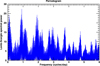 |
Fig. 6 Lomb-Scargle periodogram displaying spectral power versus frequency. The frequency is given in cycles per day so that potential 24 h aliases are easy to identify by their regular spacing. The most prominent peak occurs at 0.91387408 cycles/day, equivalent to 26.26 h, but other large peaks at ~1.9 cycles/day and ~0.1 cycles/day that appear to be 24 h aliases might actually be the true periodicity. A previous period reported in the literature (Sheppard & Jewitt 2003; Thirouin et al. 2016) is compatible with the small alias seen at ~5.94 cycles/day in this plot. |
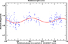 |
Fig. 7 Rotational light curve for 1995 SM55 using all photometric data, folded with a period (P) of 52.52 h. It exhibits a double-peaked profile with an amplitude of 0.05 mag. The time for phase 0.0 was chosen at the moment of mid-occultation. |
4 Results and discussion
4.1 Size and shape
The instantaneous elliptical limb fit to 1995 SM55’s projected profile (Fig. 3) yielded semi-axes a'′= 104.3 ± 0.3 km and b'′= 83.5 ± 0.5 km, with a position angle φ′ = 44.1° ± 0.4°. The goodness of fit, quantified by  , was 1.55 (Table 3). If the observed light curve intensity variations are attributed to shape effects, this suggests that 1995 SM55 deviates from a perfectly spherical form, although not dramatically, given the modest amplitude of the light curve. A triaxial ellipsoid with semi-axes a > b > c (where c is the small semi-axis and is in the spin axis direction) offers a suitable approximation for the physical body. In this section we present potential shapes and sizes of this ellipsoid by combining the occultation observations with our light curve results. According to Maclaurin spheroid theory (Chandrasekhar 1969), a hydrostatically equilibrated body rotating at approximately 52 h would adopt a Maclaurin spheroid shape with the observed axial ratio if its density were around ρ ~ 0.03 g/cm3 and ρ ~ 0.115 g/cm3 for a rotation of 26 h. Both densities are too low. On the other hand, realistic Jacobi solutions for triaxial ellipsoids in hydrostatic equilibrium are only feasible for densities that are also too low for bodies of this size range. For all the above, it is clear that 1995 SM55’s shape is not governed by hydrostatic equilibrium, as expected given that its size is well below the size needed to overcome the strength of the internal material.
Under the assumption that 1995 SM55’s shape is triaxial, we could make further analyses. The orthogonal projection of a triaxial ellipsoid (with axes a > b > c, spinning about c) for a given spin state, characterized by the aspect angle, ψ (the angle between the rotation axis c and the line of sight) and the rotational phase, ϕ, can be described as (e.g., Magnusson 1986)
 (1)
(1)
 (2)
(2)
 (3)
(3)
 (4)
(4)
where (a′, b′) denote the projected semi-axes, corresponding to the apparent semi-axes of the object’s projected cross section during a stellar occultation. A and B are the coefficients of a second degree equation in q whose solutions are the inverse of the squared semiaxes of the projected ellipse (Drummond et al. 1985). The rotational light curve amplitude for such an ellipsoid can be calculated using (e.g., Binzel et al. 1989, p. 426)
 (5)
(5)
By conducting a grid search across the three body semi-axes (a, b, c) and the polar aspect angle (ψ), and applying the rotational phase angle (ϕ) corresponding to the observed occultation time, we could identify the optimal fit to the projected shape derived from the occultation while concurrently fitting the observed rotational light curve amplitude (∆m). The rotational phase at the time of the observed occultation was 0 and the maximum brightness takes place at phase 0.91 (Fig. 7) so the rotational phase relative to the maximum of brightness is approximately 0.09 at the occultation. The observed peak-to-valley amplitude was ∆m = 0.05 ± 0.02 mag. We defined the cost function to be minimized as χ2 = (0.05 − ∆mc)2/0.022 + (1.25 − a′c/b′c)2/0.022 + (104.3 − a′c)2/0.42, where ∆mc is the modeled light curve amplitude derived from Eq. (5), and a′c, b′c are the apparent semi-axes at the rotation phase for the time of the occultation with respect to the maximum obtained from Eqs. (3)–(4) for each triaxial ellipsoid “clone” (defined by a, b, c, ψ; ϕ = 0.09 ⋅ 2π) generated during the grid search. The parameter space scanned was c = [60, 120] km, b = [c, 150] km, a = [b, 170] km, with a grid spacing of 2 km. The aspect angle ψ was varied from 0 to 90 degrees in 1° increments. This search yielded a family of potential triaxial ellipsoid solutions and aspect angles. The model that minimizes χ2 has axes  km,
km,  km,
km,  km, with an aspect angle
  . The diameter of an equal-volume sphere for this solution is Deq = 181 ± 12 km. The 1σ-uncertainties for the retrieved parameters were obtained by varying one parameter from its nominal solution value (with corresponding
  ) up to
  , while maintaining other parameters constant. In this way, the triaxial parameters derived from the light curve are consistent with those derived from the occultation.
4.2 Absolute magnitude and geometric albedo of 1995 SM55
Numerous absolute magnitude data points for 1995 SM55 are available in the literature. Doressoundiram et al. (2002) reported 4.53 ± 0.02 at a solar phase angle of 1.3°, assuming a G phase parameter of 0.15. Romanishin & Tegler (2005) provided HV = 4.54, also with an assumed G phase parameter of 0.15. Rabinowitz et al. (2008) derived 4.49 ± 0.03 with a phase slope parameter of 0.06 ± 0.03 mag/°. Jewitt et al. (2007) observed the object at a phase angle of 0.86° and applied a slope parameter of 0.04 mag/° in the R band. Using a V − R = 0.37 ± 0.07 color for this body (consistent with Belskaya et al. (2015) for 1995 SM55 and Verbiscer et al. (2022) for Haumea), the absolute magnitude becomes 4.67. Peixinho et al. (2012) quoted HR = 4.352, which, with the addition of the V − R value of 0.37, yields HV = 4.73. Absolute magnitudes in 𝑔, r, i, z bands are also presented by Ofek (2012) in their Table 3. Transforming these 𝑔riz magnitudes to UBVRI using the equations available online7 results in an absolute magnitude in V of 4.67.
Our own photometric database, comprising over 400 observations collected spanning more than 10 years, yields an absolute magnitude of 4.55 ± 0.01 with a phase slope parameter of 0.04 ± 0.02. We find no notable long-term variations within the observation period, which suggests that the spin axis’s orientation relative to an Earth observer has remained largely unchanged. Since our observations cover a wide range of phase angles and a substantial time span, effectively smoothing out rotational variability, we still have confidence in our absolute magnitude determination, which is also consistent with the average of literature values. Given our use of Gaia DR3 stars as calibrators and transformation equations accurate to approximately 0.02 mag, our final estimate is 4.55 ± 0.03 mag.
The geometric albedo (pV) and diameter (D) of a small Solar System body are linked by the following relation (e.g., Russell 1916; Harris 1998):
 (6)
(6)
where HV is the object’s absolute magnitude,  , and V⊙ is the Sun’s apparent V magnitude. Standard values for V⊙ include −26.76 (Willmer 2018) and −26.74 (Rieke et al. 2008), which lead to D0 values of 1330.2 km and 1342.6 km, respectively. An older, commonly cited value is D0 = 1329 km.
Applying Eq. (6) with D0 = 1330.2 km and our derived area-equivalent diameter D = 186.7 km, and using the absolute magnitude HV = 4.55 derived in this work (corrected for the rotational phase at the time of the occultation by 0.02 mag using the rotational light curve shown in Fig. 7), we obtain a geometric albedo of 0.80 ± 0.04. The geometric albedo of Haumea coming from occultation results is reported as 0.51 ± 0.02 (Ortiz et al. 2017). Dunham et al. (2019) later refined the 3D shape of Haumea proposed by Ortiz et al. (2017), suggesting a slightly smaller body in terms of equivalent diameter (both rotational average and volume-equivalent) compared to the original estimate. Based on this reduced size, they proposed a higher albedo of 0.66. However, it is crucial to emphasize that the geometric albedo determined by Ortiz et al. (2017) was derived directly from the accurately measured projected shape at the time of the occultation (without relying on the inferred 3D shape) and incorporated the precise instantaneous absolute magnitude measured concurrently. Therefore, no correction for a smaller overall diameter of Haumea is necessary, and the geometric albedo derived from the occultation remains accurate, with a value of 0.66 being inconsistent with these direct measurements.
Interestingly, the geometric albedo of 1995 SM55 derived in this study is higher than that of Haumea. A similar observation holds for (55636) 2002 TX300, another member of the Haumea cluster, for which an occultation of only two chords allowed an albedo determination of  (Elliot et al. 2010). Furthermore, the precise geometric albedo of Haumea’s satellite Hi’iaka, obtained from a stellar occultation, is also higher than that of Haumea (Fernández-Valenzuela et al. 2025). In all three instances, these bodies exhibit a higher geometric albedo than that of Haumea itself.
It is also recognized that the spectral water ice features of these bodies are more pronounced (Dumas et al. (2011), Pinilla-Alonso private communication), and their phase slope parameters are slightly smaller for 1995 SM55 and 2002 TX300 compared to Haumea. These differences suggest that the surface ice has distinct properties on the parent body versus its cluster members and satellites. The underlying reason for this systematic disparity remains unclear. Perhaps some mechanism has caused a darkening of Haumea’s surface relative to the surfaces of its cluster members and satellites. While collisional resurfacing of Haumea might tend to replenish its surface with fresh ice from beneath, unexposed to space weathering, it is also plausible that ejecta fallback (which is more significant for Haumea due to its higher escape velocity compared to cluster members) could darken its surface if darker material is excavated during collisional processes. Alternatively, Haumea might experience some form of internal cryovolcanism or another process that alters its surface compared to the rest of the cluster. Cryovolcanism has been hypothesized for TNOs displaying methane ice on their surfaces, such as Eris and Makemake, based on D/H ratios (Grundy et al. 2024), but Haumea lacks methane on its surface. Models concerning the collisional evolution of Haumea’s surface (Gil-Hutton et al. 2009) indicate that the high abundance of crystalline water ice relative to its amorphous phase might be explained by collisional processes, although no analysis of the effect on geometric albedo was performed. Further insight into the cause of the differing geometric albedo might come from models of multiple-scattered light on these bodies’ surfaces, incorporating various particle sizes for ices and slightly different compound mixtures compared to JWST spectra. Additionally, future occultation observations of other members of the Haumea cluster could shed more light on this issue.
4.3 Astrometry
The ellipse center coordinates presented in Table 3 constitute two of the five parameters solved for in the ellipse fit. These coordinates represent the observed-computed (O-C) offset between the observed and predicted position (defined by the ephemeris and the star’s position). This information is then used to determine the astrometric position of the object. We derived an astrometric position (ICRS) for 1995 SM55 at 2024-02-25 18:13:53.460 UT for a geocentric observer as
 (7)
(7)
 (8)
(8)
This high-precision astrometry can be employed to determine the TNO’s orbit with enhanced accuracy, which will subsequently improve the precision of future occultation predictions.
5 Conclusions
For the first time, a stellar occultation by the TNO 1995 SM55, a recognized member of the Haumea orbital cluster, was accurately predicted, subsequently refined, and successfully observed. Making use of seven occultation chords gathered from five distinct observing sites, we determined the object’s instantaneous projected shape and size by fitting an elliptical profile with semi-axis dimensions of (104.3 ± 0.3) × (83.5 ± 0.5) km. The computed area-equivalent diameter (Deq,A) at the time of the occultation is 186.7 ± 1.8 km.
Additionally, our study yielded an absolute magnitude (HV) of 4.55 ± 0.03, a V − R color of 0.37 ± 0.05, and a phase slope of 0.04 ± 0.02 mag/°. These values are consistent with prior research. Furthermore, we attempted to ascertain this TNO’s rotation period from our extensive photometric observation campaigns. However, a definitive rotation period could not be established with certainty. Our preferred rotation period (P) is 52.52 ± 0.02 hours or 26.26 ± 0.01 hours. The light curve is either double-peaked or single-peaked, a distinction that could not be conclusively made, exhibiting a peak-to-valley amplitude (∆m) of 0.05 ± 0.02 mag.
By integrating the occultation data with the rotational light curve results, we derived some constraints on 1995 SM55’s 3D size and shape. Nevertheless, these constraints remain weak due to significant uncertainties in the aspect angle and rotational properties.
From the derived area-equivalent diameter (Deq,A) of 186.7 ± 1.8 km, the aforementioned absolute magnitude, and applying a 0.02 mag correction for the rotational phase at the time of the occultation, we calculated a geometric albedo (pV) of 0.80 ± 0.04. This value is notably higher than the geometric albedo reported for Haumea. This trend also appears to extend to other members of the Haumea orbital cluster and its satellites, suggesting systematic differences in the ice composition or properties covering their surfaces compared to Haumea. Finally, we successfully derived an occultation-based astrometric position (ICRS) for (24835) 1995 SM55 (Sect. 4.3).
Acknowledgements
This work was supported by multiple funding agencies and institutions. It was partly funded by the Spanish projects PID2020-112789GB-I00 (AEI) and Proyecto de Excelencia de la Junta de Andalucía PY20-01309. J.L.O., P.S.-S., N.M., A.A.C. and R.D. acknowledge financial support from the Severo Ochoa grant CEX2021-001131-S (MCIN/AEI/10.13039/501100011033). P.S.-S. also acknowledges support from the Spanish I+D+i project PID2022-139555NB-I00 (TNO-JWST) funded by MCIN/AEI/10.13039/501100011033. AAC acknowledges financial support from the project PID2023-153123NB-I00 funded by MCIN/AEI. Gy.M.Sz. acknowledges the SNN-147362, GINOP-2.3.2-15-2016-00003, and K-138962 grants of the Hungarian Research, Development and Innovation Office (NKFIH). Z.G. acknowledges the PRODEX Experiment Agreement No. 4000137122 between ELTE Eötvös Loránd University and ESA, the VEGA grant No. 2/0031/22 of the Slovak Academy of Sciences, the Slovak Research and Development Agency contract No. APVV-20-0148, and support from the city of Szombathely. J.I.B.C. acknowledges CNPq grants 305917/2019-6 and 306691/2022-1, and FAPERJ grant 201.681/2019. F.B.R. acknowledges CNPq grant 316604/2023-2. This study was financed in part by CAPES (Finance Code 001) and the National Institute of Science and Technology of the e-Universe project (INCT do e-Universo, CNPq grant 465376/2014-2). A. Takey and A.M. Abdelaziz acknowledge financial support from the Egyptian Science, Technology & Innovation Funding Authority (STDF) under grant 48102. M.A. acknowledges grants 427700/2018-3, 310683/2017-3, and 473002/2013-2. The work of A.S. and D.A.N. was supported by a grant of the Ministry of Research, Innovation and Digitalization (CCCDI – UEFISCDI, project PN-IV-P6-6.3-SOL-2024-2-0220, within PNCDI IV). D.I. acknowledges funding provided by the University of Belgrade – Faculty of Mathematics through grant 451-03-136/2025-03/200104 from the Ministry of Science, Technological Development and Innovation of the Republic of Serbia. V.N. acknowledges support from the Bando Ricerca Fondamentale INAF 2023 Data Analysis Grant: “Characterization of transiting exoplanets by exploiting the unique synergy between TASTE and TESS”. Operation of the University of Haifa’s H80 telescope at the Wise Observatory is partly supported by ISF grant 3200/20. .IST60 and .IST40 are observational facilities of Istanbul University Observatory, funded by the Istanbul University Scientific Research Projects Coordination Unit (projects BAP-3685 and FBG-2017-23943) and by the Presidency of Strategy and Budget of the Republic of Türkiye (project 2016K12137). This work is partly based on observations collected at the Centro Astronómico Hispano en Andalucía (CAHA), Observatorio de Sierra Nevada (IAA-CSIC), and the Liverpool Telescope at the Roque de los Muchachos Observatory (IAC). This research has made use of data from the European Space Agency (ESA) mission Gaia (https://www.cosmos.esa.int/gaia), processed by the Gaia Data Processing and Analysis Consortium (https://www.cosmos.esa.int/web/gaia/dpac/consortium), with funding provided by institutions participating in the Gaia Multilateral Agreement. The authors thank Peter C. Slansky and M. Krahn for their observational contribution, and gratefully acknowledge all observers who attempted to observe this occultation event but are not explicitly mentioned in Table A.1. They also thank their collaborators at the University of Athens Observatory for utilizing the robotic Cassegrain reflector (see Gazeas (2016) for details).
Appendix A Observation details
Observation details for the February 25, 2024, occultation by 1995 SM55.
References
- Belskaya, I. N., Barucci, M. A., Fulchignoni, M., & Dovgopol, A. N. 2015, Icarus, 250, 482 [Google Scholar]
- Binzel, R., Gehrels, T., & Matthews, M. 1989, Asteroids II, Asteroids II No. v. 1 (University of Arizona Press) [Google Scholar]
- Braga-Ribas, F., Sicardy, B., Ortiz, J. L., et al. 2014, Nature, 508, 72 [NASA ADS] [CrossRef] [Google Scholar]
- Brown, M. E., Barkume, K. M., Ragozzine, D., & Schaller, E. L. 2007, Nature, 446, 294 [NASA ADS] [CrossRef] [Google Scholar]
- Chandrasekhar, S. 1969, Ellipsoidal Figures of Equilibrium, Lectures (Silliman Foundation) (Yale University Press) [Google Scholar]
- Desmars, J., Camargo, J. I. B., Braga-Ribas, F., et al. 2015, A&A, 584, A96 [NASA ADS] [CrossRef] [EDP Sciences] [Google Scholar]
- Doressoundiram, A., Peixinho, N., de Bergh, C., et al. 2002, AJ, 124, 2279 [NASA ADS] [CrossRef] [Google Scholar]
- Drummond, J. D., Cocke, W. J., Hege, E. K., & Strittmatter, P. A. 1985, Icarus, 61, 132 [NASA ADS] [CrossRef] [Google Scholar]
- Dumas, C., Carry, B., Hestroffer, D., & Merlin, F. 2011, A&A, 528, A105 [NASA ADS] [CrossRef] [EDP Sciences] [Google Scholar]
- Dunham, E. T., Desch, S. J., & Probst, L. 2019, ApJ, 877, 41 [NASA ADS] [CrossRef] [Google Scholar]
- Elliot, J. L., Person, M. J., Zuluaga, C. A., et al. 2010, Nature, 465, 897 [NASA ADS] [CrossRef] [Google Scholar]
- Farkas-Takács, A., Kiss, Cs., Vilenius, E., et al. 2020, A&A, 638, A23 [NASA ADS] [CrossRef] [EDP Sciences] [Google Scholar]
- Fernández-Valenzuela, E., Ortiz, J. L., Morales, N., et al. 2025, Nat. Commun., accepted, in press [Google Scholar]
- Ferreira, J. F., Tanga, P., Spoto, F., Machado, P., & Herald, D. 2022, A&A, 658, A73 [NASA ADS] [CrossRef] [EDP Sciences] [Google Scholar]
- Gault, D., Nosworthy, P., Nolthenius, R., Bender, K., & Herald, D. 2022, Minor Planet Bull., 49, 3 [Google Scholar]
- Gazeas, K. 2016, in Revista Mexicana de Astronomia y Astrofisica Conference Series, 48, 22 [Google Scholar]
- Gil-Hutton, R., Licandro, J., Pinilla-Alonso, N., & Brunetto, R. 2009, A&A, 500, 909 [NASA ADS] [CrossRef] [EDP Sciences] [Google Scholar]
- Gomes-Júnior, A. R., Morgado, B. E., Benedetti-Rossi, G., et al. 2022, MNRAS, 511, 1167 [CrossRef] [Google Scholar]
- Grundy, W. M., Wong, I., Glein, C. R., et al. 2024, Icarus, 411, 115923 [NASA ADS] [CrossRef] [Google Scholar]
- Harris, A. W. 1998, Icarus, 131, 291 [Google Scholar]
- Horner, J., Evans, N. W., & Bailey, M. E. 2004, MNRAS, 354, 798 [NASA ADS] [CrossRef] [Google Scholar]
- Hubbard, W. B., Hunten, D. M., Dieters, S. W., Hill, K. M., & Watson, R. D. 1988, Nature, 336, 452 [NASA ADS] [CrossRef] [Google Scholar]
- Jewitt, D., Peixinho, N., & Hsieh, H. H. 2007, AJ, 134, 2046 [Google Scholar]
- Kaminski, K., Weber, C., Marciniak, A., Zolnowski, M., & Gedek, M. 2023, PASP, 135, 025001 [CrossRef] [Google Scholar]
- Kervella, P., Thévenin, F., Di Folco, E., & Ségransan, D. 2004, A&A, 426, 297 [NASA ADS] [CrossRef] [EDP Sciences] [Google Scholar]
- Kilic, Y., Braga-Ribas, F., Kaplan, M., et al. 2022, MNRAS, 515, 1346 [NASA ADS] [CrossRef] [Google Scholar]
- Leiva, R., Buie, M. W., Keller, J. M., et al. 2020, Planet. Sci. J., 1, 48 [NASA ADS] [CrossRef] [Google Scholar]
- Lellouch, E., Santos-Sanz, P., Lacerda, P., et al. 2013, A&A, 557, A60 [NASA ADS] [CrossRef] [EDP Sciences] [Google Scholar]
- Lomb, N. R. 1976, Astrophys. Space Sci., 39, 447 [Google Scholar]
- Magnusson, P. 1986, Icarus, 68, 1 [NASA ADS] [CrossRef] [Google Scholar]
- Morales, N., Ortiz, J. L., Morales, R., et al. 2022, in European Planetary Science Congress, EPSC2022-664 [Google Scholar]
- Morgado, B. E., Sicardy, B., Braga-Ribas, F., et al. 2023, Nature, 614, 239 [NASA ADS] [CrossRef] [Google Scholar]
- Müller, T. G., Lellouch, E., Böhnhardt, H., et al. 2009, Earth Moon Planet, 105, 209 [CrossRef] [Google Scholar]
- Müller, T., Lellouch, E., & Fornasier, S. 2020, in The Trans-Neptunian Solar System, eds. D. Prialnik, M. A. Barucci, & L. Young, 153 [Google Scholar]
- Ofek, E. O. 2012, ApJ, 749, 10 [NASA ADS] [CrossRef] [Google Scholar]
- Oliveira, J. M., Sicardy, B., Gomes-Júnior, A. R., et al. 2022, A&A, 659, A136 [NASA ADS] [CrossRef] [EDP Sciences] [Google Scholar]
- Ortiz, J. L., Thirouin, A., Campo Bagatin, A., et al. 2012, MNRAS, 419, 2315 [NASA ADS] [CrossRef] [Google Scholar]
- Ortiz, J. L., Duffard, R., Pinilla-Alonso, N., et al. 2015, A&A, 576, A18 [NASA ADS] [CrossRef] [EDP Sciences] [Google Scholar]
- Ortiz, J. L., Santos-Sanz, P., Sicardy, B., et al. 2017, Nature, 550, 219 [NASA ADS] [CrossRef] [Google Scholar]
- Ortiz, J. L., Santos-Sanz, P., Licandro, J., & Pravec, P. 2019, in EPSC-DPS Joint Meeting 2019, EPSC-DPS2019-1458 [Google Scholar]
- Ortiz, J. L., Sicardy, B., Camargo, J. I. B., Santos-Sanz, P., & Braga-Ribas, F. 2020, in The Trans-Neptunian Solar System, eds. D. Prialnik, M. A. Barucci, & L. Young, 413 [Google Scholar]
- Peixinho, N., Delsanti, A., Guilbert-Lepoutre, A., Gafeira, R., & Lacerda, P. 2012, A&A, 546, A86 [NASA ADS] [CrossRef] [EDP Sciences] [Google Scholar]
- Pravec, P., Fatka, P., Vokrouhlický, D., et al. 2018, Icarus, 304, 110 [Google Scholar]
- Rabinowitz, D. L., Schaefer, B. E., Schaefer, M., & Tourtellotte, S. W. 2008, AJ, 136, 1502 [Google Scholar]
- Rieke, G. H., Blaylock, M., Decin, L., et al. 2008, AJ, 135, 2245 [NASA ADS] [CrossRef] [Google Scholar]
- Romanishin, W., & Tegler, S. C. 2005, Icarus, 179, 523 [Google Scholar]
- Rommel, F. L., Braga-Ribas, F., Desmars, J., et al. 2020, A&A, 644, A40 [NASA ADS] [CrossRef] [EDP Sciences] [Google Scholar]
- Russell, H. N. 1916, ApJ, 43, 173 [Google Scholar]
- Sarid, G., Volk, K., Steckloff, J. K., et al. 2019, ApJ, 883, L25 [Google Scholar]
- Scargle, J. D. 1982, ApJ, 263, 835 [Google Scholar]
- Schlichting, H. E., & Sari, R. 2009, ApJ, 700, 1242 [Google Scholar]
- Sheppard, S. S., & Jewitt, D. C. 2003, Earth Moon Planets, 92, 207 [Google Scholar]
- Sheppard, S. S., Lacerda, P., & Ortiz, J. L. 2008, in The Solar System Beyond Neptune, eds. M. A. Barucci, H. Boehnhardt, D. P. Cruikshank, A. Morbidelli, & R. Dotson, 129 [Google Scholar]
- Sicardy, B., Widemann, T., Lellouch, E., et al. 2003, Nature, 424, 168 [NASA ADS] [CrossRef] [Google Scholar]
- Thirouin, A., Sheppard, S. S., Noll, K. S., et al. 2016, AJ, 151, 148 [Google Scholar]
- Verbiscer, A. J., Helfenstein, P., Porter, S. B., et al. 2022, PSJ, 3, 95 [NASA ADS] [Google Scholar]
- Vilenius, E., Stansberry, J., Müller, T., et al. 2018, A&A, 618, A136 [NASA ADS] [CrossRef] [EDP Sciences] [Google Scholar]
- Willmer, C. N. A. 2018, ApJS, 236, 47 [Google Scholar]
- Zacharias, N., Monet, D. G., Levine, S. E., et al. 2004, in American Astronomical Society Meeting Abstracts, 205, 48.15 [Google Scholar]
The (clockwise-positive) angle between the “g-positive” direction (i.e., north) and the semiminor axis, b′.
All Tables
Occultation circumstances and target star parameters for (24835) 1995 SM55 on February 25, 2024.
All Figures
|
Fig. 1 Map of the ground track from our refined prediction, which incorporated astrometry acquired at the 1.5 m Sierra Nevada telescope, the 1.2 m Calar Alto telescope, and the 2 m Liverpool telescope. The blue lines mark the boundaries of the body’s shadow, calculated assuming a spherical shape with a diameter (D) of 398 km. The central path is indicated by a green line. Red lines illustrate the 3-sigma uncertainties associated with the prediction. The map also shows the observation sites: green markers denote positive detections, red negative detections (i.e., “misses”), blue planned but unexecuted observations, yellow locations with adverse weather, and purple technical problems. Map credit: OpenStreetMap. |
| In the text | |
|
Fig. 2 Occultation light curves from the various instruments that successfully registered the event. The light curves (flux versus time) are normalized to one, with an arbitrary offset applied for enhanced clarity. Dots represent the observational data, while the lines correspond to the model as described in Sect. 2. The Chalin light curve (pink) is enlarged the inset. |
| In the text | |
|
Fig. 3 Left: positive chords obtained from the sites indicated in the legend. Red segments illustrate the 1σ uncertainties originating from errors in ingress and egress times. Note that the large uncertainties come from the fact that the detector was at readout when the star reappeared. Continuous gray lines denote locations where negative data were obtained. Right: elliptical fit to the chords from the February 25, 2024, occultation. This fit characterizes the limb of 1995 SM55 as projected onto the sky plane, defined by the (f, g) axes with origin on the NIMA v10 ephemeris, at the moment of the occultation. The two chords obtained using the T100 and RTT150 telescopes at the Türkiye National Observatories are graphically indistinguishable in these plots, as are those from the two telescopes at Wise Observatory. The gray shaded area represents the 3σ-uncertainty region of the derived ellipse. |
| In the text | |
|
Fig. 4 Grazing light curve at Chalin (black dots) together with a model fit (red line) as described in the text. The light curve (flux versus time) clearly shows diffraction spikes at both disappearance and reappearance. |
| In the text | |
|
Fig. 5 Reduced magnitude, mV (1, 1, α), plotted against the phase angle, α. A total of 649 observations, obtained with the 2 m Liverpool telescope, the 1.5 m telescope at Sierra Nevada Observatory, and the 1.2 m telescope at Calar Alto Observatory, were analyzed. This plot was constructed after applying a sigma-clip rejection for outliers and selecting images with a signal-to-noise ratio greater than 30. |
| In the text | |
|
Fig. 6 Lomb-Scargle periodogram displaying spectral power versus frequency. The frequency is given in cycles per day so that potential 24 h aliases are easy to identify by their regular spacing. The most prominent peak occurs at 0.91387408 cycles/day, equivalent to 26.26 h, but other large peaks at ~1.9 cycles/day and ~0.1 cycles/day that appear to be 24 h aliases might actually be the true periodicity. A previous period reported in the literature (Sheppard & Jewitt 2003; Thirouin et al. 2016) is compatible with the small alias seen at ~5.94 cycles/day in this plot. |
| In the text | |
|
Fig. 7 Rotational light curve for 1995 SM55 using all photometric data, folded with a period (P) of 52.52 h. It exhibits a double-peaked profile with an amplitude of 0.05 mag. The time for phase 0.0 was chosen at the moment of mid-occultation. |
| In the text | |
Current usage metrics show cumulative count of Article Views (full-text article views including HTML views, PDF and ePub downloads, according to the available data) and Abstracts Views on Vision4Press platform.
Data correspond to usage on the plateform after 2015. The current usage metrics is available 48-96 hours after online publication and is updated daily on week days.
Initial download of the metrics may take a while.