| Issue |
A&A
Volume 703, November 2025
|
|
|---|---|---|
| Article Number | A12 | |
| Number of page(s) | 11 | |
| Section | Extragalactic astronomy | |
| DOI | https://doi.org/10.1051/0004-6361/202556652 | |
| Published online | 31 October 2025 | |
The nebular phase of SN 2024ggi: A low-mass progenitor with no signs of interaction
1
Instituto de Astrofísica de La Plata (UNLP – CONICET), Paseo del Bosque S/N, 1900 Buenos Aires, Argentina
2
Facultad de Ciencias Astronómicas y Geofísicas, Universidad Nacional de La Plata, Paseo del Bosque S/N, B1900FWA La Plata, Argentina
3
Kavli Institute for the Physics and Mathematics of the Universe (WPI), The University of Tokyo, Kashiwa, 277-8583 Chiba, Japan
4
Finnish Centre for Astronomy with ESO (FINCA), 20014 University of Turku, Finland
5
Tuorla Observatory, Department of Physics and Astronomy, 20014 University of Turku, Finland
6
Institute for Astronomy, University of Hawai’i at Manoa, 2680 Woodlawn Dr., Hawai’i, HI 96822, USA
7
Planetary Science Institute, 1700 E. Fort Lowell Rd, Ste 106, Tucson, AZ 85719, USA
8
Hamburger Sternwarte, Gojenbergsweg 112, 21029 Hamburg, Germany
9
Homer L. Dodge Dept. of Physics and Astronomy, University of Oklahoma, 440 W. Brooks, Rm 100, Norman, OK 73019, USA
10
Observatories of the Carnegie Institution for Science, 813 Santa Barbara Street, Pasadena, CA 91104, USA
11
Institute of Space Sciences (ICE-CSIC), Campus UAB, Carrer de Can Magrans, s/n, E-08193 Barcelona, Spain
12
Institut d’Estudis Espacials de Catalunya (IEEC), 08860 Castelldefels (Barcelona), Spain
13
Department of Astronomy, Kyoto University, Kitashirakawa-Oiwake-cho, Sakyo-ku, Kyoto 606-8502, Japan
14
Las Campanas Observatory, Carnegie Observatories, Casilla 601, La Serena, Chile
15
Department of Physics and Astronomy, Aarhus University, Ny Munkegade 120, DK-8000 Aarhus C, Denmark
16
Department of Physics, Florida State University, 77 Chieftan Way, Tallahassee, FL 32306, USA
⋆ Corresponding authors: This email address is being protected from spambots. You need JavaScript enabled to view it.
; This email address is being protected from spambots. You need JavaScript enabled to view it.
Received:
29
July
2025
Accepted:
3
September
2025
Abstract
Context. SN 2024ggi is a Type II supernova (SN) discovered in the nearby galaxy NGC 3621 (D ≈ 6.7 ± 0.4 Mpc) on 2024 April 03.21 UT. Its proximity has prompted a detailed investigation of the SN’s properties and its progenitor star. This work focuses on the optical evolution of SN 2024ggi at the nebular phase.
Aims. We investigate the progenitor properties and possible asymmetries in the ejecta by studying the nebular phase evolution between days 287 and 400 after the explosion.
Methods. We present the optical photometry and spectroscopy of SN 2024ggi during the nebular phase, obtained with the Las Campanas and Gemini South Observatories. Four nebular spectra were taken at 287, 288, 360, and 396 days post-explosion, supplemented by late-time uBVgri-band photometry spanning 320–400 days. The analysis of the nebular emission features was performed to probe the ejecta asymmetries. Based on the [O I] flux and [O I]/[Ca II] ratio, coupled with comparisons with spectra models from the literature, we arrived at an estimate of the progenitor mass. Additionally, we constructed the bolometric light curve from optical photometry and near-infrared data to derive the synthesized nickel mass.
Results. Our analysis suggests a progenitor zero-age main sequence mass between 12 − 15 M⊙. The late-time bolometric light curve is consistent with a synthesized 56Ni mass of 0.05 − 0.06 M⊙. The line profiles exhibit only minor changes over the observed period, suggesting roughly symmetrical ejecta, with a possible clump of oxygen-rich material moving towards the observer. There were no signatures of circumstellar material interaction detected up to 400 days after the explosion.
Key words: supernovae: general / supernovae: individual: SN 2024ggi
© The Authors 2025
 Open Access article, published by EDP Sciences, under the terms of the Creative Commons Attribution License (https://creativecommons.org/licenses/by/4.0), which permits unrestricted use, distribution, and reproduction in any medium, provided the original work is properly cited.
This article is published in open access under the Subscribe to Open model. This email address is being protected from spambots. You need JavaScript enabled to view it. to support open access publication.
1. Introduction
Core-collapse supernovae (CCSNe) mark the demise of massive stars with initial masses ≳8 M⊙. The majority of these explosions are classified as hydrogen-rich Type II SNe (Li et al. 2011). They are believed to arise from stars in the red supergiant (RSG) phase that managed to retain a substantial hydrogen-rich envelope. Observationally, the association with RSG stars has been supported by direct progenitor identifications in archival images (Van Dyk et al. 2003; Maund et al. 2005). In spite of the well-established connection with RSGs, there are still major uncertainties related to their initial masses and evolutionary paths. The zero-age main sequence (ZAMS) mass of the progenitor star plays a decisive role in governing its evolutionary path and the resulting SN observational features.
Despite the efforts engaged across a number observational and theoretical works, there are still many significant unknowns around the progenitor mass distribution of SNe. On one hand, there is uncertainty around the lower limiting mass for core-collapse and this limit value varies depending on the numerical modeling and physical parameters of the star, such as metallicity, rotation, mass-loss rates, and mixing processes (Eldridge & Tout 2004; Ibeling & Heger 2013). On the other hand, while stellar evolution models predict that stars up to ∼25 M⊙ would be expected to undergo successful CC explosions, pre-SN observations of RSGs indicate an apparent upper mass limit of only ∼17 M⊙ (Smartt et al. 2009). This tension, known as the RSG problem, suggests either (1) a fundamental gap in our understanding of late-stage massive stellar evolution (e.g., enhanced mass loss Crowther 2007, binary interactions Podsiadlowski et al. 2004; Smith 2014, or fallback-induced black hole formation MacFadyen et al. 2001) or (2) systematic biases in progenitor detection and mass determination. In this context, it becomes essential to obtain increasingly precise progenitor mass determinations through both improved pre-explosion imaging and detailed modeling of supernova light curves and spectra, particularly for events occurring in nearby galaxies with well-characterized stellar populations.
Another principal factor governing the evolution of high-mass stars is their mass loss. This mass loss can be driven by line-driven winds, eruptive episodes, and/or binary interactions. These processes not only shape the stellar evolution, but also create extensive circumstellar material (CSM) which the SN ejecta subsequently interact with. Such interactions are manifested observationally through an early light curve evolution (Förster et al. 2018), high luminosities and blue colors at early times (Jacobson-Galán et al. 2024a), X-ray and radio emission (Chevalier & Fransson 2017; Moriya 2021), highly ionized emission features in early-time spectra (known as flash features; Gal-Yam et al. 2014; Khazov et al. 2016; Yaron et al. 2017; Bruch et al. 2021; Jacobson-Galán et al. 2022), and strong, boxy emission profiles in late-time spectra (Kotak et al. 2009; Weil et al. 2020; Folatelli et al. 2025; Jacobson-Galán et al. 2025).
Constraining both the progenitor masses and their mass-loss histories is therefore essential for understanding the final evolutionary stages and explosion mechanisms of massive stars. The nebular phase, beginning ∼100 − 150 days post-explosion, when the ejecta become optically thin, provides particularly valuable diagnostics. During this phase, photons from the innermost regions escape, revealing the explosion geometry and nucleosynthetic products. Observed asymmetries in the nebular emission lines may reflect intrinsic asymmetries in the explosion itself, offering clues to the progenitor’s structure and explosion dynamics. Late-time modeling of SNe spectra has provided another tool to investigate the progenitor properties and, more specifically, the progenitor masses (Jerkstrand et al. 2012; Dessart et al. 2021). Recent work by Fang et al. (2025a) has further addressed the RSG problem by demonstrating that nebular spectral analysis supports the absence of high-mass RSG progenitors, reinforcing the possibility of revising stellar evolution models.
SN 2024ggi, discovered on April 11, 2024, by the Asteroid Terrestrial-impact Last Alert System (ATLAS; Tonry et al. 2018) in NGC 3621, represents a pivotal case study. With a first detection at JD = 2460411.64 (Tonry et al. 2024; Chen et al. 2025) and a rapid classification as a Type II SN (Hoogendam et al. 2024; Zhai et al. 2024), it stands alongside SN 2023ixf as one of the nearest and most intensively observed core-collapse SNe in recent years (see e.g., Jacobson-Galán et al. 2023; Kilpatrick et al. 2023; Bersten et al. 2024; Ferrari et al. 2024).
Its proximity and early discovery have enabled intensive monitoring campaigns, resulting in high-cadence ultraviolet, optical, and infrared (IR) observations. The SN presented flash ionized features, as reported by Hoogendam et al. (2024), Zhang et al. (2024), Pessi et al. (2024), Jacobson-Galán et al. (2024b), and Shrestha et al. (2024). Multiwavelength follow-up efforts yielded X-ray detections within the first three days post-explosion (Margutti & Grefenstette 2024; Lutovinov et al. 2024; Zhang et al. 2024) and a radio counterpart weeks later (Ryder et al. 2024), while no significant emission was found in the centimeter and millimeter range (Chandra et al. 2024; Hu et al. 2025), nor in γ-rays (Marti-Devesa & Fermi-LAT Collaboration 2024). Baron et al. (2025) reported IR observations obtained with the James Webb Space Telescope (JWST) and ground-based telescopes during the plateau phase, ∼55 days after the explosion.
The archival image analyses showed a progenitor candidate consistent with an RSG star. Xiang et al. (2024) combined Hubble Space Telescope (HST) and Spitzer Space Telescope pre-explosion images to characterize the progenitor as a bright, red star with an estimated initial mass of 13 ± 1 M⊙. Chen et al. (2024), using Dark Energy Camera Legacy Survey data, independently proposed a slightly more massive progenitor (14 − 17 M⊙). An alternative approach by Hong et al. (2024) leveraged HST imaging to analyze the local stellar environment. By dating the youngest stellar population near the supernova site, they inferred a progenitor mass of 10.2 M⊙, providing a complementary estimate to direct detection methods. Ertini et al. (2025) presented the first hydrodynamical model of the bolometric light curve during the full plateau phase and derived a progenitor mass of 15 M⊙. Lastly, a recent work by Dessart et al. (2025) proposes that the nebular features in the optical and NIR spectra are aptly reproduced by a progenitor of M = 15.2 M⊙.
This paper is organized as follows. Section 2 presents our observational dataset, including details of the data reduction procedures and the adopted reddening and distance parameters. In Section 3, we describe our detailed analysis of the nebular-phase spectra, with a particular emphasis on emission line profiles and their implications for ejecta geometry. Section 4 examines the late-time light curve evolution and provides estimates of the synthesized 56Ni mass. We explain how we derived progenitor mass constraints from the nebular spectra in Sect. 5. Finally, Sect. 6 synthesizes our key findings and discusses their implications, placing SN 2024ggi in context with both previous progenitor studies and our current understanding of Type II SNe.
2. Observations, reddening, and distance
This work is based on spectroscopic and photometric data acquired at the Gemini South Observatory and the Las Campanas Observatory. The spectra acquired at the Las Campanas Observatory were taken by the Precision Observations of Infant Supernova Explosions (POISE1, Burns et al. 2021) collaboration. Phases presented in this paper are referred to an explosion date of JD = 2460411.295 ± 0.345, which corresponds to the midpoint between the first detection of the SN (JD = 2460411.64, Tonry et al. 2024) and the last non-detection (JD = 2460410.95, Killestein et al. 2024). The heliocentric redshift of the host galaxy reported by Koribalski et al. (2004) is zHel = 0.0024, which is the value we adopted throughout the work to correct the spectra and the light-curve phases.
The distance to NGC 3621 was measured by Paturel et al. (2002) using the Cepheid period-luminosity relation, yielding D = 6.7 ± 0.5 Mpc. An independent determination by Saha et al. (2006) obtained D = 7.4 ± 0.4 Mpc through a similar methodology. Given the comparable uncertainties between the two measurements, we adopted the former value to maintain consistency with the analysis of Ertini et al. (2025), facilitating a direct comparison of the results.
Several independent studies have estimated the host galaxy extinction for this source using different methods. Following the calibration from Stritzinger et al. (2018), Jacobson-Galán et al. (2024b) derived E(B − V)host = 0.084 ± 0.018 mag by analyzing the Na I D1 and D2 equivalent widths in high-resolution spectra. In contrast, Pessi et al. (2024) and Shrestha et al. (2024) obtained lower values of E(B − V)host = 0.036 ± 0.007 mag and 0.034 ± 0.020 mag, respectively, using the relations from Poznanski et al. (2012). When combined with the Milky Way’s contribution, the total extinction estimates from these studies are consistent due to a different treatment of the Milky Way extinction contribution. Jacobson-Galán et al. (2024b) reported E(B − V)tot = 0.154 mag, while Pessi et al. (2024) found 0.16 mag and Shrestha et al. (2024) found 0.154 mag. Given the uncertainties in these values, we adopt the coincident total reddening of E(B − V)tot = 0.16 mag for our analysis using the Cardelli et al. (1989) law with Rv = 3.1.
2.1. Spectra
Two optical spectra were taken with the Inamori-Magellan Areal Camera & Spectrograph (IMACS, Dressler et al. 2011), mounted at the 6.5 m Baade telescope, on 2025 January 23 and 2025 April 06 UT, 286.8 and 359.6 rest-frame days relative to the explosion date given above. All spectra were acquired with the grism Gri-300-17.5; the first one consisted of two 600 s exposures, while the last one consisted of two 900 s exposures. The dispersion of both spectra is ≈5 Å; thus, the spectral resolution is ≈250 km s−1 at 6000 Å.
Another spectrum was obtained with the Gemini Multi-Object Spectrograph (GMOS; Hook et al. 2004) mounted on the Gemini South Telescope (Program GS-2025A-Q-120, PI Ferrari) on 2025 January 24 UT, 287.7 rest-frame days after the explosion. The observations were divided into four 900 s exposures in long-slit mode with the R400 grating. The data were processed with standard procedures using the IRAF Gemini package. The flux calibration was performed with a baseline standard observation. The spectrum dispersion is ≈10 Å, resulting in a spectral resolution of ≈500 km s−1 at 6000 Å.
The last epoch was taken on 2025 May 12 and 13 UT, with the Low Dispersion Survey Spectrograph (LDSS3, upgraded from LDSS2, Allington-Smith et al. 1994) mounted on the 6.5 m Clay Telescope of the Las Campanas Observatory. We combined both spectra and obtained a single epoch, which, on average, is 395.9 rest-frame days after the explosion date. The grism used was the VPH-ALL, with a slit of 1 arcsec. Both observations consisted of four 300-s exposures each. The dispersion is ≈8.5, which represents a spectral resolution of ≈400 km s−1 at 6000 Å. All four spectra are plotted in Fig. 1 (see top panel) and normalized by the maximum in the [O I] λλ6300, 6364 region.
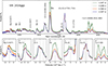 |
Fig. 1. Top panel: SN 2024ggi nebular spectra at 287, 288, 360, and 396 days after the explosion. The 288 d (GMOS) spectrum is plotted with a thin line as it is almost the same epoch as the 287 d (IMACS) spectrum (we do not combine them as they were taken with different instruments). Bottom panels: Line profiles at 287, 360, and 396 days in the velocity space for (a) Mg I]λ4571, (b) Na I D, (c) [O I]λλ6300, 6364, (d) Hα, (e) [Fe II]λ7155, f) [Ca II]λλ7291, 7324, and (g) Ca II T. For the purposes of visualization, all the spectra are scaled to the maximum emission in the [O I] region. |
2.2. Light curves
The photometry presented in this work was acquired with the 1-m Henrietta Swope Telescope of the Las Campanas Observatory. The follow-up spans February 25 and April 26, 2025, that is, roughly between 320 and 400 d in the BVgri filters, and until 377 d in the u band. The temporal cadence varies with time between 1 to 14 days for the later observations. The reduction was performed with the POISE photometric pipeline, which is based on the Carnegie Supernova Project (CSP) pipeline described in Contreras et al. (2010) and Krisciunas et al. (2017). The resulting photometry calibrated to the natural system of the Swope Telescope is listed in Table 2 and shown in Fig. 4.
The Gemini Program GS-2025A-Q-120 included three 30 s exposures in both the g′ and r′ bands, which were used to calibrate the spectrum. These provided two additional points to the light curve dated January 24th, 2025, which was 288.4 days after the explosion. The images were reduced using the Dragons software2 (Labrie et al. 2023). We performed the photometry measurements of the SN using the Autophot Python package (Brennan & Fraser 2022), which employs point-spread function (PSF) photometry for sources with signal-to-noise ratio (S/N) above our detection threshold of 25. The instrumental magnitudes were calibrated to the standard Sloan system using zero points derived from field stars from the Pan-STARRS catalog (Flewelling et al. 2020). We included data from the Asteroid Terrestrial-impact Last Alert System (ATLAS; Tonry et al. 2018) downloaded from its public forced photometry service3 (Smith et al. 2020).
3. Spectral properties
3.1. Overall description
Figure 1 presents the spectrum obtained with GMOS, the two IMACS spectra, and the LDSS3 spectrum. The lower panels illustrate the dominant features in velocity space. Over the time interval covered by the observations, the supernova exhibits slow evolution, with the line profiles retaining their shapes while gradually declining in flux. Figure 2 shows a comparison between SN 2024ggi and other Type II supernovae. The selected objects were chosen based on their high data quality, extensive temporal coverage, and their classification as representative Type II SNe.
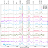 |
Fig. 2. Nebular spectra of SN 2024ggi compared with SN 2023ixf, SN 2004et and SN 199em. All spectra have been corrected by their reported redshift and scaled by the mean value in the region between 7600 − 8400 Å. Emission lines are marked in gray dotted lines. |
The spectra at 287 and 288 days are overplotted, as they are nearly indistinguishable. The spectra of SN 2024ggi display the characteristic emission lines expected for a Type II SN in the nebular phase, with the primary emissions arising from oxygen, hydrogen, calcium, iron, and sodium ions.
The strongest emission lines are centered at their rest wavelengths. Notably, Hα remains nearly at rest, and its flux diminishes more rapidly than that of other lines. A detailed analysis of the [O I] and Hα features is provided in Sect. 3.2.
When compared to the extensive sample of Type II SNe from Silverman et al. (2017), the nebular spectra of SN 2024ggi appear typical, though with some subtle distinctions. The Hα profile is marginally broader than usual (see Sect. 3.2) and the [O I] doublet exhibits a persistent single-peaked profile throughout the observed period. This profile likely reflects the spatial distribution of the ejecta, as discussed further in Sect. 3.2.
Finally, we note the lack of an emission feature between [O I] and Hα, detected in SN 2023ixf (Fig. 2) and attributed to relatively early CSM interaction (Kumar et al. 2025; Folatelli et al. 2025; Fang et al. 2025b). This absence suggests that contrary to SN 2023ixf, SN 2024ggi did not experience interaction between rapidly expanding SN ejecta with circumstellar material. However, extended spectroscopic monitoring beyond 600–700 days will be essential to determine whether late-phase interaction features emerge, as observed in some normal Type II SNe (Kotak et al. 2009; Weil et al. 2020).
3.2. Line profiles and ejecta asymmetries
The Mg I] λ4571 emission exhibits an asymmetric profile, with a peak that gradually evolves toward the blue, and a weakening of the red wing (see Fig. 1, panel a). The Na I D line maintains a residual P Cygni profile with noticeable asymmetry (Fig. 1, panel b). This line might suffer from contamination due to He Iλ5876.
The [O I] λλ6300,6364 doublet displays a persistent single-peaked profile throughout our observations, accompanied by a narrow emission component blue-shifted by ≈ − 1200 km s−1 (see Fig. 1, panel c). While the blue shift gradually decreases with time, the full width at half maximum (FWHM) of the broad component remains constant. Figure 1 (panel c) demonstrates that the [O I] profile maintains its complex morphology throughout our observations. We present detailed Gaussian fits to the 287 days spectrum in Fig. 3, with corresponding parameters listed in Table 1. Panel a) depicts a three-component fitting, consisting of a broad central emission (FWHM ≈5000 km s−1 blue shifted by ≈600 km s−1) combined with a narrow component (FWHM ≈1400 km s−1) that evolves from −1300 to −1100 km s−1 (although this difference lies within our spectral resolution; see Sect. 2). An additional component accounts for the red shoulder, which may include contamination from a weak Hα P Cygni profile. Panel b), on the other hand, shows a four-component alternative, for which we constrained the doublet separation to 64 Å, finding both primary components blueshifted by ≈900 km s−1, while the narrow emission and red shoulder features remain consistent with the three-component approach. However, in this case, the ratio [O I]λ6300/[O I]λ6364 would be 1 : 1, which implies an optically thick regime, not expected for the nebular phase.
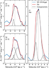 |
Fig. 3. Gaussian decomposition of the [O I]λλ6300, 6364 and Hα line profiles in the spectrum of SN 2024ggi at 287 days. Panel (a): Three-Gaussian fitting of the [O I] doublet, with a wide component centered nearly at the rest wavelength (i.e., 6300 Å). Panel (b): Four-Gaussian fitting of the [O I] doublet with the separation of the two wide emissions fixed at 64 Å. Panel (c): Three-Gaussian fitting of the Hα line, resulting in a wide component centered at rest. In Table 1, all FWHM and peak velocity values are detailed for the three fittings. |
A single Gaussian does not fit the Hα line well due to its pronounced asymmetry. A single-component fit yields central velocities near rest with FWHM values of 3900, 3800, and 3700 km s−1 at 287, 360, and 396 days, respectively. Our preferred three-component model (Fig. 3, panel c) includes a central emission (FWHM ≈ 3100 km s−1) at rest wavelength, a blue shifted component (≈1600 km s−1, FWHM ≈ 1500 km s−1), and a red component. While these velocities do not align with [N II] doublet positions, we cannot exclude the possibility of some contribution from the [N II] and Fe II permitted lines. This multi-component structure likely reflects intrinsic line asymmetry rather than distinct emitting regions, possibly indicating a persistent P Cygni absorption affecting the blue wing.
The [Fe II] λ7155 feature is particularly noteworthy because it has a stable double-peaked profile at all epochs, with velocity components at ≈1000 km s−1 and −1200 km s−1 (see Fig. 1, panel e). This distinctive structure is absent in our comparison sample (Fig. 2) and, to our knowledge, it has not been previously reported in Type II SNe. The uniqueness of the profile may reflect either an asymmetric distribution of iron-rich ejecta (as discussed in Fang et al. 2024) or a self-absorption effect. Hueichapán et al. (2025) reported the presence of double-peak features in other [Fe II] lines in the IR, further supporting the hypothesis that this phenomenon arises from asphericity in the ejecta.
The [Ca II] profile shows three persistent peaks at 7280 Å, 7310 Å, and 7340 Å (see Fig. 1, panel f). Interpreting the two redder features as doublet components implies a ≈500 km s−1 blue shift. Alternatively, using the mean doublet wavelength (7307 Å) as reference would imply a central component near the rest, blue, and red components shifted by −1000 km s−1 and 1500 km s−1, respectively. Notably, the Ca II NIR triplet fades more rapidly than other lines, with the redder component decaying slightly slower than its bluer counterparts (see Fig. 1, panel g).
The overall line profiles suggest that the ejecta is relatively symmetric. The notable exception is the blue-shifted [O I] component, which could indicate a localized clump of oxygen-rich material moving toward the observer. The fact that the FWHMs of the [O I] and the Hα lines are similar (see Table 1) might indicate substantial mixing of the H-rich envelope with the core material.
4. Late-time light curves and 56Ni mass
4.1. Late-time decline rates
Between 200 and 400 days, the light curves follow the expected linear decline pattern for Type II SNe. A distinct break appears in the r- and i-band light curves at approximately 365 days, marking the onset of a slightly faster decline rate. This behavior is reflected in the ATLAS o-band data, while the bluer BVgc bands (and potentially the u band) maintain a nearly constant decline rate throughout the entire observed period (see Fig. 4).
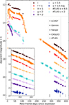 |
Fig. 4. Optical light curves of SN 2024ggi. The new data published in this work correspond to the Gemini and Swope telescopes. The early phase data is reported in Ertini et al. (2025). The black vertical lines indicate the phases of the four spectra presented in this work. The dotted gray line indicates the epoch where the o-, r-, and i-band light curves show a slope break, also noticeable in the ATLAS o-band light curve (see Sect. 4). Inset shows an expanded view of the temporal evolution between 320 − 415 days, highlighting the change in decline rate. Solid lines represent separate linear fits to the data before and after 365 days (marked by the vertical dotted line). |
We quantified the decline rates through linear fits to each band, with uncertainties determined via Monte Carlo simulations using 5000 iterations. The resulting measurements, presented in Table 3, reveal statistically significant slope changes for the o-, r-, and i-bands following the 365-day break point. Before that phase, all values are equal to or lower than that of the decline rate in the case of full γ-ray trapping, that is, 1 mag per 100 days.
Photometry of the SN 2024ggi spanning from 320 to 380 days after the explosion, obtained with the Henrietta Swope Telescope at Las Campanas Observatory.
Decline rate in all filters for SN 2024ggi in mag/100 d, before and after the break at 365 days.
As we discuss in Sect. 3.2, the Hα and Ca II NIR triplet fluxes drop faster than other lines such as the [O I] and [Ca II] doublets. We tested whether this change in line fluxes could be responsible for the increase in the decline rates seen in the ori bands, as opposed to a change in the continuum shape. The change in decline rates seen in the ori bands may in part be attributed to a sudden drop in the Hα and Ca II NIR triplet line fluxes. A rough calculation based on the difference between the 397 and the 287 days spectra scaled to the same epoch by the 56Co decline rate indicates that the decrease in line fluxes is enough to explain the drop in the ori-band fluxes between the extrapolations that result using the pre- and post-356 d decline rates. However, the cause of the sudden change in flux (whether it be line or continuum) remains unclear.
4.2. Bolometric luminosity and Ni mass
During the radioactive tail phase of Type II SNe, the bolometric luminosity is primarily governed by the mass of synthesized 56Ni. By this stage, hydrogen recombination in the ejecta iscomplete, and the emission is powered exclusively by the radioactive decay 56Co → 56Fe (Anderson 2019). The deposition of energy from 56Co decay products (γ rays and positrons) heats the ejecta and sustains the observed emission. A steeper light-curve decline relative to the instantaneous 56Co decay rate may indicate partial leakage of gamma rays from the ejecta.
Additional mechanisms, such as ejecta-CSM interaction, dust formation, or light echoes, could influence the late-time light curve evolution. However, our analysis of the spectral and photometric data up to 400 days post-explosion shows no evidence of substantial ongoing interaction, as demonstrated by the absence of interaction features. Similarly, the lack of significant dust formation is inferred from the stability of the emission line profiles. This interpretation is further supported by the absence of dust-related features in late-time IR spectra, as reported by Dessart et al. (2025). Light echoes, which typically produce a bluer flux excess, would also be expected to flatten the late-time light curve in blue filters. Instead, we observed a continued decline in these bands, ruling out any significant contribution from echoes. We therefore assume that the late-time emission is dominated by the radioactive decay input, thus neglecting any additional effects.
Our late-time photometry covers the optical wavelength range. At this phase, an important fraction of the total flux from the SN is emitted in the IR range of the electromagnetic spectrum (beyond 8000Å, see e.g., Dessart 2025). To compute an accurate bolometric flux, we used spectra from the Infrared Telescope Facility (IRTF), dated February 15, 2025 (310 days) and from the JWST, taken on January 21, 2025 (287 days). These data will be published by Mera et al (in prep.), with details on the reduction procedure published in Medler et al. (2025), Hoogendam et al. (2025a,b).
The IRTF and JWST spectra overlap in the region between 1.7 and 2.3 μm. Using the absolutely flux-calibrated JWST spectrum as reference, we scaled the IRTF spectrum to match the mean flux level in this overlapping region. This procedure enabled us to construct a continuous, flux-calibrated IR spectrum spanning 0.9-4.1 μm at 287 days.
After obtaining a combined IRTF+JWST spectrum, we derived synthetic photometry in the Swope BVgri bands from our reddening-corrected IMACS spectrum at 287 days (previously flux-scaled using contemporaneous photometry; see Sect. 2). This enabled the construction of a complete spectral energy distribution (SED) spanning 0.44 to 3.5 μm. We computed the total bolometric flux by integrating the synthetic magnitudes and adding estimated UV (< 0.44 μm) and far-IR (> 3.5 μm) contributions derived from a blackbody fit to the SED. Remarkably, 60% of the total flux originated outside the optical BVgri bands, with 50% emerging in the IR and 10% in the UV.
We further assumed that this percentage remained constant throughout the entire tail phase. This assumption is justified by black-body fits to the Swope photometry between 320 and 395 days, which yielded a nearly constant black-body inferred temperature of TBB = 4200 − 4500 K. Additionally, the slow evolution of optical spectral features suggests that no strong variations in emission lines outside this wavelength range would significantly alter the derived percentages.
Finally, we computed the bolometric luminosity by integrating the SED over the observed Swope bands, adding the 60% flux total. The resulting bolometric light curve is presented in Fig. 5. The decline rates were calculated with the same methodology used for the optical filters, and are also specified in Table 3. We did not note a significant break at 365 days, as noticed in the ori bands. Instead, the resulting slopes closely match the expected decline rate of the 56Co decay, and suggest a high efficiency in γ-ray trapping within the ejecta.
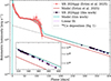 |
Fig. 5. Bolometric light curve of SN 2024ggi. The bolometric light curve published in Ertini et al. (2025) and their preferred model are plotted in pink dots and line, respectively. Our fitting of Eq. (1) is shown in purple. A new hydrodynamical model with the same parameters as those presented in Ertini et al. (2025), but with a larger 56Ni mass of 0.052 M⊙ is shown in the cyan line. The dashed gray line indicates the decay with a 56Ni mass of 0.049 M⊙ and full-trapping of γ rays. |
To estimate the synthesized 56Ni mass, we adopted the methodology of Hamuy (2003), which assumes complete trapping of γ-rays by the ejecta. This assumption may not hold if the ejecta becomes sufficiently diffuse at late times. To account for potential γ-ray escape, we incorporated the prescription proposed by Clocchiatti & Wheeler (1997), where the observed luminosity is decreased dependent on the γ-ray escape timescale, tγ.
Combining these approaches yields
![Mathematical equation: $$ \begin{aligned} M_{Ni} = (7.866 \times 10^{-44})\ \frac{L(t)}{1-\exp (-(t_{\gamma }/t)^2)}\ \exp {\left[\frac{t - 6.1}{111.26}\right]} \ M_\odot , \end{aligned} $$](/articles/aa/full_html/2025/11/aa56652-25/aa56652-25-eq1.gif) (1)
(1)
where Lt represents the bolometric luminosity (in erg s−1) at the rest-frame epoch, t. We derived the 56Ni mass and gamma-ray escape timescale by fitting the bolometric light curve obtaining MNi = 0.049 M⊙ and tγ = 561 days, respectively. This high value is consistent with the decline rate of the bolometric light curve, confirming nearly complete γ-ray trapping.
A potential limitation of this method lies in the accuracy of the SED integration, particularly given the emission-line-dominated nature of the spectrum. To assess this, we compared the integration over the full spectral range with that of synthetic flux points from the observed spectra and found the discrepancy to be less than 5%, confirming the robustness of ourapproach.
As an additional validation, we used the pseudo-bolometric luminosity (pLbol) of SN 1987A as a reference, fitting the following relation,
 (2)
(2)
where t denotes the rest-frame time since explosion in days and tγ represents the γ-ray escape timescale as in Eq. (1) (see, e.g., Spiro et al. 2014). We adopted a redshift of z = 0.001 for SN 1987A, while for SN 2024ggi we used the redshift value reported in Sect. 2.
We computed the pseudo-bolometric luminosity pLbol(t) for SN 1987A by integrating its flux over the BVRI bands (Whitelock et al. 1988). To match the photometric systems of the observations of SN 1987A and SN 2024ggi, we performed synthetic photometry in the Johnson system using flux-scaled spectra of SN 2024ggi. This allowed us to derive the transformation factors between the Sloan and Johnson systems, which we subsequently applied to all photometric data. From this analysis, we obtained a 56Ni mass of MNi = 0.059 M⊙ and a γ-ray escape timescale of tγ = 553 days for SN 2024ggi.
Finally, we compared the late-time bolometric light curve with a suite of hydrodynamical models computed using the one-dimensional Lagrangian local thermodynamic equilibrium radiation hydrodynamics code from Bersten et al. (2011). Fig. 5 displays the preferred model published by Ertini et al. (2025) (15 M⊙ progenitor, 56Ni mass of 0.035 M⊙) alongside a model with the same progenitor, explosion energy, and CSM parameters and a higher 56Ni mass (0.052 M⊙). While the lower-mass model shows a strong disagreement with the observed light curve, the second model provides a better match.
Our estimates, derived from three independent methods, are mutually consistent, resulting in a 56Ni mass of 0.05 − 0.06 M⊙, which is significantly higher than the 0.035 M⊙ value reported by Ertini et al. (2025, the only published estimate to date). This discrepancy likely stems from uncertainties in their bolometric light curve construction beyond 85 days, which relied solely on (B − V) color-based bolometric corrections from Martinez et al. (2022). Such an approach is subject to large uncertainties, while our approach is more robust. Dessart et al. (2025) propose a model with a 56Ni mass of 0.06 M⊙ that, despite it not being fitted, reproduces the observed optical and NIR spectra at late times.
5. Progenitor mass
Nebular spectra are strongly dependent on the mass of the progenitor star. As a consequence, there are several methods to derive progenitor initial masses from nebular features. Our first method resides in estimating an oxygen core mass from the [O I] λλ6300, 6364 luminosity, which is then linked to the progenitor mass through oxygen production yields (Uomoto 1986; Jerkstrand et al. 2014; Kuncarayakti et al. 2015). Nevertheless, a few caveats must be considered. This emission arises from the neutral oxygen, so the derived progenitor mass is a lower limit and higher ionization levels must be assumed to be able to estimate a total oxygen mass. This procedure also depends strongly on the absolute flux calibration of the spectrum and on the estimate of the materials’ temperature. The [O I] λ5577 line is an indicator of this temperature (see e.g., Jerkstrand et al. 2014), but it is not recognizable in the spectra of SN 2024ggi presented here, as it appears blended with other emission lines. Instead, we assume the material follows a temperature evolution similar to the model from Jerkstrand et al. (2014) for SN 2012aw. In SN 2024ggi, the [O I] doublet flux decreases slowly with time. The measured flux from the 287, 360, and 396 d spectra are 2.21 × 10⁻¹³, 1.52 × 10⁻¹³, and 1.15 × 10⁻¹³ erg s−1 cm−2, respectively. At the distance of the SN, this implies an oxygen mass of 0.3 M⊙. When compared to theoretical oxygen production yields from Rauscher et al. (2002) and Ertl et al. (2020), this suggests a ZAMS mass well below the minimum mass included in their models of 15 M⊙. For those values calculated by Nomoto et al. (1997) and Limongi & Chieffi (2003), the progenitor must have been a star between 12 and 15 M⊙. Fig. 6 shows the cited production yields and our oxygen core mass estimations for the three epochs.
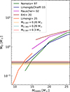 |
Fig. 6. Oxygen core mass estimated from the measurement of the [O I] doublet for phases 287, 360, and 396 days (horizontal lines). Oxygen production yields published by Nomoto et al. (1997), Rauscher et al. (2002), Limongi & Chieffi (2003), Ertl et al. (2020), and Limongi et al. (2025) point to an initial mass of 12 − 15 M⊙ for the progenitor star. |
The [O I]/[Ca II] ratio has been suggested as a more reliable indicator of the progenitor mass (Fransson & Chevalier 1989; Kuncarayakti et al. 2015; Fang et al. 2019, 2022), as it does not depend on the absolute flux calibration of the spectrum. Moreover, this value does not change significantly during the evolution, making this method less sensitive to the observation epoch. In addition, the ratio is apparently unaffected by possible interaction between the SN ejecta and surrounding material (Folatelli et al. 2025). The progenitor mass can be constrained by comparing the flux ratio with those from synthetic spectra. In SN 2024ggi, the measured ratios were 0.48 ± 0.07, 0.49 ± 0.09, and 0.48 ± 0.07 for each epoch, respectively. Compared with models from Jerkstrand et al. (2014) and Dessart et al. (2021), these values correspond to a somewhat low mass progenitor, around 10 − 12 M⊙.
Another way of arriving at a mass estimation is by directly comparing the observed spectra with synthetic spectra from the literature, such as those published by Dessart et al. (2021) and Jerkstrand et al. (2012). In Fig. 7, we show a comparison of our observed spectra with the series of model spectra computed for varying initial progenitor masses at similar ages. The models that better match the SN emission lines correspond to relatively low masses, of 12 and 15 M⊙. Higher mass models are shown to significantly overproduce the oxygen and sodium features.
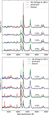 |
Fig. 7. SN 2024ggi in comparison with synthetic spectra from Jerkstrand et al. (2014) and Dessart et al. (2021). All the spectra are scaled by the mean value between 6900 − 8200 Å as an indication of the continuum. The upper plot shows the spectra at 288 days, while the synthetic spectra phases are 360 and 250 days for the Dessart et al. (2021) and Jerkstrand et al. (2014) models, respectively. In the bottom plot, we show our last spectrum at 396 days, this time changing spectra from Jerkstrand et al. (2014) with those at the phase of 400 days. |
6. Conclusions
We present optical photometric and spectroscopic observations of the nearby Type II SN 2024ggi during its nebular phase. The dataset includes four spectra obtained at 287, 288, 360, and 397 days after the explosion, along with uBVgri photometry spanning days 320 to 400. The observations were conducted at the Gemini Observatory and Las Campanas Observatory. This comprehensive dataset enabled us to investigate both the explosion properties and the nature of the progenitor star, yielding a progenitor mass estimate that is independent from those previously published.
The nebular spectra display the characteristic emission features of Type II SNe, with prominent forbidden lines of oxygen, calcium, and (semi-forbidden) magnesium, as well as strong Hα and the Ca II infrared triplet. While most emission features exhibit single-peaked, symmetric profiles, the [Fe II] λ7155 line shows a distinct double-peaked structure. The line profiles overall suggest a roughly spherical ejecta geometry, with minimal Doppler shifts and little temporal evolution. No signatures of late-time interaction with circumstellar material, such as variability in Hα or excess emission on the blue part of the spectrum, were detected up to 400 days post-explosion.
The late-time light curves decline at a rate of approximately 1 mag per 100 days across all filters, consistent with the expected behavior of Type II SNe. A notable break appears in the redder bands around day 365, potentially indicating a decline in the strength of Hα and calcium features relative to the continuum. Using near-infrared data (Mera et al., in prep.), we constructed the bolometric light curve and inferred a 56Ni mass of ≈0.05 − 0.06 M⊙, significantly higher than the 0.035 M⊙ reported by Ertini et al. (2025). We attribute this discrepancy to the large uncertainties in the methodology for computing the second half of the bolometric light curve in that work.
To constrain the progenitor mass, we compared our spectra with nebular models from Jerkstrand et al. (2014) and Dessart et al. (2021). Both direct spectral comparisons and the [O I]/[Ca II] flux ratio suggest a progenitor initial mass of 10 − 15 M⊙. From the luminosity of the [O I] line alone, we estimated an oxygen core mass of 0.26 − 0.30 M⊙, which corresponds to an initial mass below 15 M⊙ based on oxygen yields from Rauscher et al. (2002) and Ertl et al. (2020). Using nucleosynthesis models from Nomoto et al. (1997), Limongi & Chieffi (2003), and the more recent yields from Limongi et al. (2025), we were able to refine this to a progenitor with MZAMS between 12 and 15 M⊙.
Our progenitor mass estimate is consistent with previous studies. Xiang et al. (2024) reported a mass of 13 ± 1 M⊙, and Ertini et al. (2025) suggest 15 M⊙, both consistent with our results. While Hong et al. (2024) found a slightly lower mass of 10.2 M⊙, the value derived by Chen et al. (2024) is slightly higher, in the range of 14 − 17 M⊙. Further optical and infrared observations will be essential to studying potential dust formation and the eventual onset of interaction between the ejecta and the surrounding CSM.
Acknowledgments
The authors thank Dr. Carlos Contreras for his contribution to this work by obtaining observational data with the Clay Magellan Telescope at Las Campanas Observatory. L. F. acknowledges financial support from Consejo Nacional de Investigaciones Científicas y Técnicas (CONICET). L.G. acknowledges financial support from AGAUR, CSIC, MCIN and AEI 10.13039/501100011033 under projects PID2023-151307NB-I00, PIE 20215AT016, CEX2020-001058-M, ILINK23001, COOPB2304, and 2021-SGR-01270. K.M. acknowledges support from NASA grants JWST-GO-02114, JWST-GO-02122, JWST-GO-04522, JWST-GO-04217, JWST-GO-04436, JWST-GO-03726, JWST-GO-05057, JWST-GO-05290, JWST-GO-06023, JWST-GO-06677, JWST-GO-06213, JWST-GO-06583. Support for programs #2114, #2122, #3726, #4217, #4436, #4522, #5057, #6023, #6213, #6583, and #6677 were provided by NASA through a grant from the Space Telescope Science Institute, which is operated by the Association of Universities for Research in Astronomy, Inc., under NASA contract NAS 5-03127. Some of this material is based upon work supported by the National Science Foundation Graduate Research Fellowship Program under Grant Nos. 1842402 and 2236415. Any opinions, findings, conclusions, or recommendations expressed in this material are those of the author(s) and do not necessarily reflect the views of the National Science Foundation. M.D. Stritzinger is funded by the Independent Research Fund Denmark (IRFD, grant number 10.46540/2032-00022B) and by an Aarhus University Research Foundation Nova project (AUFF-E-2023-9-28).
References
- Allington-Smith, J., Breare, M., Ellis, R., et al. 1994, PASP, 106, 983 [Google Scholar]
- Anderson, J. P. 2019, A&A, 628, A7 [NASA ADS] [CrossRef] [EDP Sciences] [Google Scholar]
- Baron, E., Ashall, C., DerKacy, J. M., et al. 2025, ArXiv e-prints [arXiv:2507.18753] [Google Scholar]
- Bersten, M. C., Benvenuto, O., & Hamuy, M. 2011, ApJ, 729, 61 [NASA ADS] [CrossRef] [Google Scholar]
- Bersten, M. C., Orellana, M., Folatelli, G., et al. 2024, A&A, 681, L18 [NASA ADS] [CrossRef] [EDP Sciences] [Google Scholar]
- Brennan, S. J., & Fraser, M. 2022, A&A, 667, A62 [NASA ADS] [CrossRef] [EDP Sciences] [Google Scholar]
- Bruch, R. J., Gal-Yam, A., Schulze, S., et al. 2021, ApJ, 912, 46 [NASA ADS] [CrossRef] [Google Scholar]
- Burns, C., Hsiao, E., Suntzeff, N., et al. 2021, ATel., 14441, 1 [Google Scholar]
- Cardelli, J. A., Clayton, G. C., & Mathis, J. S. 1989, ApJ, 345, 245 [Google Scholar]
- Chandra, P., Maeda, K., Nayana, A. J., et al. 2024, ATel., 16612, 1 [Google Scholar]
- Chen, X., Kumar, B., Er, X., et al. 2024, ApJ, 971, L2 [Google Scholar]
- Chen, T.-W., Yang, S., Srivastav, S., et al. 2025, ApJ, 983, 86 [Google Scholar]
- Chevalier, R. A., & Fransson, C. 2017, in Handbook of Supernovae, eds. A. W. Alsabti, & P. Murdin, 875 [Google Scholar]
- Clocchiatti, A., & Wheeler, J. C. 1997, ApJ, 491, 375 [Google Scholar]
- Contreras, C., Hamuy, M., Phillips, M. M., et al. 2010, AJ, 139, 519 [Google Scholar]
- Crowther, P. A. 2007, ARA&A, 45, 177 [Google Scholar]
- Dessart, L. 2025, A&A, in press, https://doi.org/10.1051/0004-6361/202555664 [Google Scholar]
- Dessart, L., Hillier, D. J., Sukhbold, T., Woosley, S. E., & Janka, H. T. 2021, A&A, 652, A64 [NASA ADS] [CrossRef] [EDP Sciences] [Google Scholar]
- Dessart, L., Kotak, R., Jacobson-Galan, W., et al. 2025, A&A, submitted [arXiv:2507.05803] [Google Scholar]
- Dressler, A., Bigelow, B., Hare, T., et al. 2011, PASP, 123, 288 [NASA ADS] [CrossRef] [Google Scholar]
- Eldridge, J. J., & Tout, C. A. 2004, MNRAS, 353, 87 [NASA ADS] [CrossRef] [Google Scholar]
- Ertini, K., Regna, T. A., Ferrari, L., et al. 2025, A&A, 699, A60 [NASA ADS] [CrossRef] [EDP Sciences] [Google Scholar]
- Ertl, T., Woosley, S. E., Sukhbold, T., & Janka, H. T. 2020, ApJ, 890, 51 [CrossRef] [Google Scholar]
- Fang, Q., Maeda, K., Kuncarayakti, H., Sun, F., & Gal-Yam, A. 2019, Nat. Astron., 3, 434 [Google Scholar]
- Fang, Q., Maeda, K., Kuncarayakti, H., et al. 2022, ApJ, 928, 151 [NASA ADS] [CrossRef] [Google Scholar]
- Fang, Q., Maeda, K., Kuncarayakti, H., & Nagao, T. 2024, Nat. Astron., 8, 111 [Google Scholar]
- Fang, Q., Moriya, T. J., & Maeda, K. 2025a, ApJ, 986, 39 [Google Scholar]
- Fang, Q., Moriya, T. J., Ferrari, L., et al. 2025b, ApJ, 978, 36 [NASA ADS] [CrossRef] [Google Scholar]
- Marti-Devesa, G., & Fermi-LAT Collaboration 2024, ATel., 16601, 1 [Google Scholar]
- Ferrari, L., Folatelli, G., Ertini, K., Kuncarayakti, H., & Andrews, J. E. 2024, A&A, 687, L20 [NASA ADS] [CrossRef] [EDP Sciences] [Google Scholar]
- Flewelling, H. A., Magnier, E. A., Chambers, K. C., et al. 2020, ApJS, 251, 7 [NASA ADS] [CrossRef] [Google Scholar]
- Folatelli, G., Ferrari, L., Ertini, K., Kuncarayakti, H., & Maeda, K. 2025, A&A, 698, A213 [NASA ADS] [CrossRef] [EDP Sciences] [Google Scholar]
- Förster, F., Moriya, T. J., Maureira, J. C., et al. 2018, Nat. Astron., 2, 808 [CrossRef] [Google Scholar]
- Fransson, C., & Chevalier, R. A. 1989, ApJ, 343, 323 [NASA ADS] [CrossRef] [Google Scholar]
- Gal-Yam, A., Arcavi, I., Ofek, E. O., et al. 2014, Nature, 509, 471 [CrossRef] [Google Scholar]
- Hamuy, M. 2003, ApJ, 582, 905 [NASA ADS] [CrossRef] [Google Scholar]
- Hong, X., Sun, N.-C., Niu, Z., et al. 2024, ApJ, 977, L50 [Google Scholar]
- Hoogendam, W., Auchettl, K., Tucker, M., et al. 2024, Transient Name Server AstroNote, 103, 1 [Google Scholar]
- Hoogendam, W. B., Ashall, C., Jones, D. O., et al. 2025a, ApJ, 988, 209 [Google Scholar]
- Hoogendam, W. B., Jones, D. O., Ashall, C., et al. 2025b, Open J. Astrophys., 8, 120 [Google Scholar]
- Hook, I. M., Jørgensen, I., Allington-Smith, J. R., et al. 2004, PASP, 116, 425 [NASA ADS] [CrossRef] [Google Scholar]
- Hu, M., Ao, Y., Yang, Y., et al. 2025, ApJ, 978, L27 [Google Scholar]
- Hueichapán, E., Cartier, R., Prieto, J. L., et al. 2025, ArXiv e-prints [arXiv:2508.02656] [Google Scholar]
- Ibeling, D., & Heger, A. 2013, ApJ, 765, L43 [NASA ADS] [CrossRef] [Google Scholar]
- Jacobson-Galán, W. V., Dessart, L., Jones, D. O., et al. 2022, ApJ, 924, 15 [CrossRef] [Google Scholar]
- Jacobson-Galán, W. V., Dessart, L., Margutti, R., et al. 2023, ApJ, 954, L42 [CrossRef] [Google Scholar]
- Jacobson-Galán, W. V., Dessart, L., Davis, K. W., et al. 2024a, ApJ, 970, 189 [CrossRef] [Google Scholar]
- Jacobson-Galán, W. V., Davis, K. W., Kilpatrick, C. D., et al. 2024b, ApJ, 972, 177 [CrossRef] [Google Scholar]
- Jacobson-Galán, W. V., Dessart, L., Davis, K. W., et al. 2025, ApJ, 992, 100 [Google Scholar]
- Jerkstrand, A., Fransson, C., Maguire, K., et al. 2012, A&A, 546, A28 [NASA ADS] [CrossRef] [EDP Sciences] [Google Scholar]
- Jerkstrand, A., Smartt, S. J., Fraser, M., et al. 2014, MNRAS, 439, 3694 [Google Scholar]
- Khazov, D., Yaron, O., Gal-Yam, A., et al. 2016, ApJ, 818, 3 [CrossRef] [Google Scholar]
- Killestein, T., Ackley, K., Kotak, R., et al. 2024, Transient Name Server AstroNote, 101, 1 [Google Scholar]
- Kilpatrick, C. D., Foley, R. J., Jacobson-Galán, W. V., et al. 2023, ApJ, 952, L23 [NASA ADS] [CrossRef] [Google Scholar]
- Koribalski, B. S., Staveley-Smith, L., Kilborn, V. A., et al. 2004, AJ, 128, 16 [Google Scholar]
- Kotak, R., Meikle, W. P. S., Farrah, D., et al. 2009, ApJ, 704, 306 [NASA ADS] [CrossRef] [Google Scholar]
- Krisciunas, K., Contreras, C., Burns, C. R., et al. 2017, AJ, 154, 211 [NASA ADS] [CrossRef] [Google Scholar]
- Kumar, A., Dastidar, R., Maund, J. R., Singleton, A. J., & Sun, N. C. 2025, MNRAS, 538, 659 [Google Scholar]
- Kuncarayakti, H., Maeda, K., Bersten, M. C., et al. 2015, A&A, 579, A95 [CrossRef] [EDP Sciences] [Google Scholar]
- Labrie, K., Simpson, C., Cardenes, R., et al. 2023, Res. Notes Am. Astron. Soc., 7, 214 [Google Scholar]
- Li, W., Leaman, J., Chornock, R., et al. 2011, MNRAS, 412, 1441 [NASA ADS] [CrossRef] [Google Scholar]
- Limongi, M., & Chieffi, A. 2003, ApJ, 592, 404 [CrossRef] [Google Scholar]
- Limongi, M., Roberti, L., Falla, A., Chieffi, A., & Nomoto, K. 2025, ApJS, 279, 41 [Google Scholar]
- Lutovinov, A. A., Semena, A. N., Mereminskiy, I. A., et al. 2024, ATel., 16586, 1 [Google Scholar]
- MacFadyen, A. I., Woosley, S. E., & Heger, A. 2001, ApJ, 550, 410 [NASA ADS] [CrossRef] [Google Scholar]
- Margutti, R., & Grefenstette, B. 2024, ATel., 16587, 1 [Google Scholar]
- Martinez, L., Bersten, M. C., Anderson, J. P., et al. 2022, A&A, 660, A40 [NASA ADS] [CrossRef] [EDP Sciences] [Google Scholar]
- Maund, J. R., Smartt, S. J., & Danziger, I. J. 2005, MNRAS, 364, L33 [NASA ADS] [CrossRef] [Google Scholar]
- Medler, K., Ashall, C., Shahbandeh, M., et al. 2025, ArXiv e-prints [arXiv:2505.18507] [Google Scholar]
- Moriya, T. J. 2021, MNRAS, 503, L28 [Google Scholar]
- Nomoto, K., Hashimoto, M., Tsujimoto, T., et al. 1997, Nucl. Phys. A, 616, 79 [NASA ADS] [CrossRef] [Google Scholar]
- Paturel, G., Teerikorpi, P., Theureau, G., et al. 2002, A&A, 389, 19 [NASA ADS] [CrossRef] [EDP Sciences] [Google Scholar]
- Pessi, T., Cartier, R., Hueichapan, E., et al. 2024, A&A, 688, L28 [NASA ADS] [CrossRef] [EDP Sciences] [Google Scholar]
- Podsiadlowski, P., Langer, N., Poelarends, A. J. T., et al. 2004, ApJ, 612, 1044 [NASA ADS] [CrossRef] [Google Scholar]
- Poznanski, D., Prochaska, J. X., & Bloom, J. S. 2012, MNRAS, 426, 1465 [Google Scholar]
- Rauscher, T., Heger, A., Hoffman, R. D., & Woosley, S. E. 2002, ApJ, 576, 323 [Google Scholar]
- Ryder, S., Maeda, K., Chandra, P., Alsaberi, R., & Kotak, R. 2024, ATel., 16616, 1 [Google Scholar]
- Saha, A., Thim, F., Tammann, G. A., Reindl, B., & Sandage, A. 2006, ApJS, 165, 108 [Google Scholar]
- Shrestha, M., Bostroem, K. A., Sand, D. J., et al. 2024, ApJ, 972, L15 [Google Scholar]
- Silverman, J. M., Pickett, S., Wheeler, J. C., et al. 2017, MNRAS, 467, 369 [NASA ADS] [Google Scholar]
- Smartt, S. J., Eldridge, J. J., Crockett, R. M., & Maund, J. R. 2009, MNRAS, 395, 1409 [CrossRef] [Google Scholar]
- Smith, N. 2014, ARA&A, 52, 487 [NASA ADS] [CrossRef] [Google Scholar]
- Smith, K. W., Smartt, S. J., Young, D. R., et al. 2020, PASP, 132, 085002 [Google Scholar]
- Spiro, S., Pastorello, A., Pumo, M. L., et al. 2014, MNRAS, 439, 2873 [Google Scholar]
- Stritzinger, M. D., Taddia, F., Burns, C. R., et al. 2018, A&A, 609, A135 [NASA ADS] [CrossRef] [EDP Sciences] [Google Scholar]
- Tonry, J. L., Denneau, L., Heinze, A. N., et al. 2018, PASP, 130, 064505 [Google Scholar]
- Tonry, J., Denneau, L., Weiland, H., et al. 2024, Transient Name Server Discovery Report, 2024–1020, 1 [Google Scholar]
- Uomoto, A. 1986, ApJ, 310, L35 [NASA ADS] [CrossRef] [Google Scholar]
- Van Dyk, S. D., Li, W., & Filippenko, A. V. 2003, PASP, 115, 1289 [NASA ADS] [CrossRef] [Google Scholar]
- Weil, K. E., Fesen, R. A., Patnaude, D. J., & Milisavljevic, D. 2020, ApJ, 900, 11 [Google Scholar]
- Whitelock, P. A., Catchpole, R. M., Menzies, J. W., et al. 1988, MNRAS, 234, 5P [NASA ADS] [CrossRef] [Google Scholar]
- Xiang, D., Mo, J., Wang, X., et al. 2024, ApJ, 969, L15 [Google Scholar]
- Yaron, O., Perley, D. A., Gal-Yam, A., et al. 2017, Nat. Phys., 13, 510 [NASA ADS] [CrossRef] [Google Scholar]
- Zhai, Q., Li, L., Zhang, J., & Wang, X. 2024, Transient Name Server Classification Report, 2024–1031, 1 [Google Scholar]
- Zhang, J., Dessart, L., Wang, X., et al. 2024, ApJ, 970, L18 [NASA ADS] [CrossRef] [Google Scholar]
All Tables
Photometry of the SN 2024ggi spanning from 320 to 380 days after the explosion, obtained with the Henrietta Swope Telescope at Las Campanas Observatory.
Decline rate in all filters for SN 2024ggi in mag/100 d, before and after the break at 365 days.
All Figures
|
Fig. 1. Top panel: SN 2024ggi nebular spectra at 287, 288, 360, and 396 days after the explosion. The 288 d (GMOS) spectrum is plotted with a thin line as it is almost the same epoch as the 287 d (IMACS) spectrum (we do not combine them as they were taken with different instruments). Bottom panels: Line profiles at 287, 360, and 396 days in the velocity space for (a) Mg I]λ4571, (b) Na I D, (c) [O I]λλ6300, 6364, (d) Hα, (e) [Fe II]λ7155, f) [Ca II]λλ7291, 7324, and (g) Ca II T. For the purposes of visualization, all the spectra are scaled to the maximum emission in the [O I] region. |
| In the text | |
|
Fig. 2. Nebular spectra of SN 2024ggi compared with SN 2023ixf, SN 2004et and SN 199em. All spectra have been corrected by their reported redshift and scaled by the mean value in the region between 7600 − 8400 Å. Emission lines are marked in gray dotted lines. |
| In the text | |
|
Fig. 3. Gaussian decomposition of the [O I]λλ6300, 6364 and Hα line profiles in the spectrum of SN 2024ggi at 287 days. Panel (a): Three-Gaussian fitting of the [O I] doublet, with a wide component centered nearly at the rest wavelength (i.e., 6300 Å). Panel (b): Four-Gaussian fitting of the [O I] doublet with the separation of the two wide emissions fixed at 64 Å. Panel (c): Three-Gaussian fitting of the Hα line, resulting in a wide component centered at rest. In Table 1, all FWHM and peak velocity values are detailed for the three fittings. |
| In the text | |
|
Fig. 4. Optical light curves of SN 2024ggi. The new data published in this work correspond to the Gemini and Swope telescopes. The early phase data is reported in Ertini et al. (2025). The black vertical lines indicate the phases of the four spectra presented in this work. The dotted gray line indicates the epoch where the o-, r-, and i-band light curves show a slope break, also noticeable in the ATLAS o-band light curve (see Sect. 4). Inset shows an expanded view of the temporal evolution between 320 − 415 days, highlighting the change in decline rate. Solid lines represent separate linear fits to the data before and after 365 days (marked by the vertical dotted line). |
| In the text | |
|
Fig. 5. Bolometric light curve of SN 2024ggi. The bolometric light curve published in Ertini et al. (2025) and their preferred model are plotted in pink dots and line, respectively. Our fitting of Eq. (1) is shown in purple. A new hydrodynamical model with the same parameters as those presented in Ertini et al. (2025), but with a larger 56Ni mass of 0.052 M⊙ is shown in the cyan line. The dashed gray line indicates the decay with a 56Ni mass of 0.049 M⊙ and full-trapping of γ rays. |
| In the text | |
|
Fig. 6. Oxygen core mass estimated from the measurement of the [O I] doublet for phases 287, 360, and 396 days (horizontal lines). Oxygen production yields published by Nomoto et al. (1997), Rauscher et al. (2002), Limongi & Chieffi (2003), Ertl et al. (2020), and Limongi et al. (2025) point to an initial mass of 12 − 15 M⊙ for the progenitor star. |
| In the text | |
|
Fig. 7. SN 2024ggi in comparison with synthetic spectra from Jerkstrand et al. (2014) and Dessart et al. (2021). All the spectra are scaled by the mean value between 6900 − 8200 Å as an indication of the continuum. The upper plot shows the spectra at 288 days, while the synthetic spectra phases are 360 and 250 days for the Dessart et al. (2021) and Jerkstrand et al. (2014) models, respectively. In the bottom plot, we show our last spectrum at 396 days, this time changing spectra from Jerkstrand et al. (2014) with those at the phase of 400 days. |
| In the text | |
Current usage metrics show cumulative count of Article Views (full-text article views including HTML views, PDF and ePub downloads, according to the available data) and Abstracts Views on Vision4Press platform.
Data correspond to usage on the plateform after 2015. The current usage metrics is available 48-96 hours after online publication and is updated daily on week days.
Initial download of the metrics may take a while.