| Issue |
A&A
Volume 703, November 2025
|
|
|---|---|---|
| Article Number | A151 | |
| Number of page(s) | 12 | |
| Section | Galactic structure, stellar clusters and populations | |
| DOI | https://doi.org/10.1051/0004-6361/202556657 | |
| Published online | 13 November 2025 | |
First large-scale spatial and velocity patterns of local metal-rich stars in the Milky Way
1
Université Côte d’Azur, Observatoire de la Côte d’Azur, CNRS, Laboratoire Lagrange,
Nice,
France
2
Lund Observatory, Department of Geology,
Sölvegatan 12,
22362
Lund,
Sweden
3
Observational Astrophysics, Department of Physics and Astronomy, Uppsala University,
Box 516,
751 20
Uppsala,
Sweden
4
Leibniz-Institüt für Astrophysik Potsdam (AIP),
An der Sternwarte 16,
14482
Potsdam,
Germany
★ Corresponding author: This email address is being protected from spambots. You need JavaScript enabled to view it.
Received:
30
July
2025
Accepted:
18
September
2025
Abstract
Context. The present-day spatial and kinematic distribution of stars in the Milky Way provides key constraints on its internal dynamics and evolutionary history. However, identifying the correct tracers that highlight the mechanisms is far from straightforward. The best probes are stars that stand out in terms of kinematics, chemistry, or age compared to the underlying population to which they belong.
Aims. We aimed to constrain stellar radial migration and, in particular, observationally study its effect on the disc dynamical heating.
Methods. We selected Milky Way stars that are more metal-rich than the interstellar medium (ISM) at their guiding radius, the so-called local metal-rich (LMR) stars, and investigated their chemo-kinematics. Until recently, existing catalogues did not contain such targets in large quantities, but one can now select many millions of them by using Gaia photometric metallicities. We investigated their kinematics and age distributions across the disc, and compared them to the stellar populations that have the same metallicity as the ISM.
Results. Compared to locally born stars with metallicities equal to that of the ISM, LMR stars, at a given location, are always older (mean ages of up to 2 Gyr older) and with similar or slightly higher velocity dispersions. Furthermore, at a given metallicity, LMR stars are older at larger galactocentric radii, reflecting the fact that LMR stars need time to migrate. Finally, whereas we do not find any correlation between the location of the spiral arms and the spatial density of LMR stars, we do find that the mean stellar eccentricity and mean ages are lower in the spiral arms.
Conclusions. Our results support a well-established theoretical result that has not yet been formally confirmed via observations involving large datasets without modelling: churning is not significantly heating the Galactic disc. Furthermore, the age distribution of these stars rules out any significant contribution from Galactic fountains as their origin, and confirms the effect of the spiral arms on them. Although no clear signature of the Galactic bar is detected, its phase-mixed and diffuse influence – especially through interactions with spiral arms – cannot be excluded.
Key words: Galaxy: disk / Galaxy: evolution / local insterstellar matter / Galaxy: kinematics and dynamics / Galaxy: stellar content
© The Authors 2025
 Open Access article, published by EDP Sciences, under the terms of the Creative Commons Attribution License (https://creativecommons.org/licenses/by/4.0), which permits unrestricted use, distribution, and reproduction in any medium, provided the original work is properly cited.
This article is published in open access under the Subscribe to Open model. This email address is being protected from spambots. You need JavaScript enabled to view it. to support open access publication.
1 Introduction
Stellar population kinematics provide valuable insight into the dynamical processes that have taken place throughout the history of a galaxy. In particular, stars in galactic discs are thought to be born with nearly circular orbits that broadly follow the kinematics of the gas from which they were formed (e.g. Spitzer & Schwarzschild 1951; Wielen 1977). Over time, however, several processes can affect their motion, such as accretion events (e.g. Velazquez & White 1999; Kazantzidis et al. 2008; Gómez et al. 2013; Laporte et al. 2022), interactions with giant molecular clouds (Spitzer & Schwarzschild 1953; Lacey 1984; Ida et al. 1993), and resonances with non-axi-symmetries in the galactic potential, such as the bar (e.g. Di Matteo et al. 2013; Khoperskov et al. 2020; Haywood et al. 2024), the spiral arms (e.g. Minchev & Quillen 2006; Schönrich & Binney 2009), or overlapping patterns of the two (e.g. Quillen 2003; Minchev & Famaey 2010; Daniel et al. 2019; Marques et al. 2025).
At the Lindblad resonances, the eccentricity of a star increases but its guiding radius remains unchanged (e.g. Lynden-Bell & Kalnajs 1972). Such kinematically hot stars create an effect known as blurring, which causes stars to momentarily visit regions of the galaxy far from their guiding radius, with velocities lower than that of the local standard of rest if they are at their apocentre, or higher if they are at their pericentre. Resonances that occur at co-rotation tend to change the angular momentum and, hence, the guiding radius, without (much) affecting the star’s radial action (Sellwood & Binney 2002). This process is commonly called churning. The location at which co-rotation resonances occur depends on the pattern speed (and hence on the strength) of the considered structures and can change over time depending on the temporal evolution of the non-axi-symmetries (Chiba et al. 2021; Khoperskov & Gerhard 2022; Sellwood & Masters 2022; Li et al. 2024a) or the transient mass clumps provoked by the overlapping long-lived structures with different pattern speeds (Marques et al. 2025).
Whereas dynamical heating, which causes blurring, has been well established in the Milky Way since the 1970s, identified as being mostly responsible for the increase in the age-velocity dispersion relation (e.g. Wielen 1977), the first direct observational evidence of churning was only provided a decade ago by Kordopatis et al. (2015a). The authors selected stars from the medium-resolution Radial Velocity Experiment (RAVE) Data Release (DR) 4 catalogue (Kordopatis et al. 2013) with metallicities above solar in the extended solar neighbourhood (the so-called super metal-rich stars; Grenon 1972), and found that almost all had eccentricities below ~0.2, i.e. they could not just be visitors from the inner Galaxy on high eccentricity orbits. Since these stars had metallicities above the metallicity of the local interstellar medium (ISM), they could not have been born locally either, unless they were formed from locally enriched material coming from, for example, Galactic fountains (e.g. Fraternali et al. 2013; Grand et al. 2019). The presence of such stars was recently re-confirmed on a larger volume by Lehmann et al. (2024) using Gaia DR3 kinematics and Apache Point Observatory Galactic Evolution Experiment (APOGEE) DR17 metallicities and ages.
Several subsequent studies tested the efficiency of churning and its effect on the disc by selecting explicitly super metal-rich stars (e.g. Santos-Peral et al. 2021; Dantas et al. 2023; Lehmann et al. 2024), by determining the birth radii of the stars (e.g. Minchev et al. 2018; Ratcliffe et al. 2023; Lu et al. 2024), by modelling the metallicity distribution function across the disc (e.g. Lian et al. 2022), and by forward-modelling the orbit evolution for stars of a given age and metallicity and fitting it to data (Frankel et al. 2020). All these studies were based on spectroscopic surveys that overall contained only a few hundred thousand stars, a number that drops significantly when probing large distances from the Sun or the tails of the metallicity distribution function.
Nowadays, it has been collegially accepted that churning does not dynamically heat the Galactic disc, though this is based on indirect evidence and low statistics (e.g. Mackereth et al. 2019; Frankel et al. 2020; Sharma et al. 2021). That is, stars that migrate outwards via co-rotation resonances reach a given position with a similar eccentricity and maximum distance above the Galactic plane (Zmax) as locally born stars due to conservation of the radial and vertical action (Minchev et al. 2012; Halle et al. 2015; Sellwood & Binney 2025). Indeed, as stars move outwards, the Galactic potential decreases; to keep the action constant, the vertical velocity dispersion of the considered population therefore needs to decrease (see, however, Hamilton et al. 2024 and Sellwood & Binney 2025 on the spiral theories and the mechanisms that could cause this).
With the advent Gaia DR3 (Gaia Collaboration 2016, 2023c), exquisite 3D kinematics of tens of millions of stars have become available (Kordopatis et al. 2023b) and can be used to investigate these claims more thoroughly. Together with these kinematics, photometric metallicities have become available for roughly a hundred million stars thanks to state-of-the-art machine learning techniques (Andrae et al. 2023; Li et al. 2024b; Hattori 2024) and/or syntheses of cleverly chosen and calibrated photometric bands (Martin et al. 2024). Such photometric metallicities overcome problems of spectroscopy by allowing for datasets with much simpler selection effects and with homogeneously determined parameters up to relatively faint magnitudes and, hence, large distances. The synergy of the kinematic and metallicity catalogues therefore allows us to probe rare stellar populations in a unique way.
In this paper, we address the effect of churning on the disc structure using an unprecedentedly large sample of more than 1.6 · 106 local metal-rich (LMR) stars over a large volume, with Gaia DR3 kinematics and new age determinations. LMR stars are defined as having metallicities that are higher than that of today’s ISM at their guiding radius and, therefore, may not have formed locally (unless formed from infalling metal-rich material, such as the Galactic fountains). We define the ISM’s metallicity adopting the da Silva et al. (2023) metallicity log-gradient, namely [Fe/H]ISM = −0.907 · log(R) + 0.81, as evaluated using classical Cepheids and open clusters. We note that adopting other gradients, such as the linear gradients of da Silva et al. (2023) or Genovali et al. (2014), did not significantly change our results.
Section 2 describes the dataset used and the quality filters applied. Section 3 presents the results obtained for the overall kinematics and age distributions of LMR stars, and Sect. 4 describes how these results correlate with the presence of the spiral arms. Finally, Sect. 5 concludes and summarises our results.
2 Data selection
The underlying sample we used is a combination of the Gaia’s DR3 RVS sample (~33 · 106 stars, Katz et al. 2023) and the golden sample of red giant branch (RGB) star sample from Andrae et al. (2023, ~17 · 106 stars, dubbed XGBoost). The latter has photometric metallicities derived combining the CatWISE photometry together with the Gaia XP spectra and astrometry, trained adopting the labels from APOGEE DR17 (Abdurro’uf et al. 2022) and for very metal-poor stars with the labels from Li et al. (2022).
Below, we describe the different cuts we applied to this dataset. Figure A.1 summarises their successive effect on the resulting metallicity distribution.
2.1 Filtering based on Gaia astrometry and agreement with other photometric metallicities
To keep the stars with the most accurate metallicity estimates, we cross-matched our sample with the Li et al. (2024b) catalogue (dubbed AspGap). The latter also provides photometric metallicities together with global α-abundances for 37 · 106 RGB stars, derived solely based on the Gaia XP spectra and trained on both the APOGEE labels and spectra. From the resulting cross-match, we arbitrarily selected only the stars that have metallicities that agree within 0.1 dex between the two catalogues (see Fig. 1). This corresponds roughly to 69% of the cross-matched sample (~8.3 million stars out of the 11.9 million), mostly removing stars fainter than G = 13.5 mag.
We further filtered the stars based on the re-normalised unit weight error (RUWE) parameter (imposing <1.4; Lindegren 2018), to minimise the possible contamination from variable and/or multiple stars, and on the parallax uncertainty (adopting σϖ/ϖ < 0.21), to avoid positions (and hence kinematics) being strongly dependent on the distance prior of the stars (see e.g. Bailer-Jones et al. 2021). After these extra cuts, the sample consisted of 7.68 million stars.
2.2 Filtering on effective temperature
A careful investigation of the middle plots of Fig. 1 shows that very cool stars (in red) may need some further filtering to ensure a high reliability of the metallicities of the sample. To assess whether this is the case or not, we compared the selection described in the previous section with the purely spectroscopic metallicities2 from the GALactic Archaeology with HERMES (GALAH) DR4 (Buder et al. 2025). The comparison, shown in Fig. 2 (top: all of the stars with [M/H] > −1, bottom: just the LMR stars), confirms that the most discrepant stars are found to be the ones with the lowest temperatures (Teff,XGBoost ≲ 4250 K).
It is beyond the scope of this paper to assess which catalogue, XGBoost or GALAH DR4, is closer to reality (see, however, Kos et al. 2025). On the one hand, cool metal-rich stars are notoriously difficult to parameterise spectroscopically due to the multiple presence of significant absorption features formed by molecules making the continuum placement difficult (e.g. Kordopatis et al. 2011, 2023a). On the other hand, the wider wavelength coverage of the XP spectra can, in principle, lead to parameters with smaller biases than the ones obtained spectroscopically, despite the lower resolving power. However, the XGBoost parameters were obtained with a training set whose parameters were also derived spectroscopically, and photometric parameters may also be prone to degeneracies with interstellar reddening. Given these points, we therefore decided to keep only the stars in the Teff regime where there is a good agreement with GALAH, i.e. Teff, XGBoost > 4250 K. This filtering removed ~1.3 · 106 additional stars. We note that once all of the filters are applied to the data (see Fig. A.1), XGBoost’s Teff are in very good agreement with AspGap ones. As a matter of fact, the distributions of the difference between the two temperature estimates have a mean of less than 10 K and a dispersion smaller than 60 K, for the LMR subsample and the full sample (i.e. without a metallicity cut).
For the remainder of the paper, unless specified otherwise, [M/H] refers to the XGBoost metallicity.
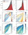 |
Fig. 1 Top: G-magnitude distributions (left) and Teff distributions (right) of the total XGBoost sample cross-matched with AspGap (in grey) and the subsample for which differences in metallicity are smaller than 0.1 dex (in red); see Sect. 2. Middle left: comparison between the XGBoost and the AspGap metallicities, colour-coded by Teff. Middle right: zoomed-in view of the high-metallicity regime. Bottom: same as the middle plots but colour-coded by the G magnitude. Black contour lines represent 33, 66, 90, and 99% of the sample. The solid red line represents the 1:1 relation, whereas the dashed ones are shifted by ±0.1 dex. |
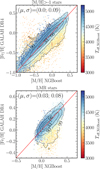 |
Fig. 2 Comparison of XGBoost metallicities with GALAH DR4 iron abundances. All of the panels include the selection described in Sect. 2.1 as well the flag_sp==0 selection from GALAH. The colour code is XGBoost Teff, and the numbers within each plot indicate the mean offset and dispersion of the difference. Top: all stars with [M/H] > −1. Bottom: LMR stars only, i.e. stars with metallicities above the ISM’s one at their guiding radius. |
2.3 Adopted positions, kinematics, and orbital parameters
We selected the positions (Galactocentric cylindrical R, and Cartesian X, Y, Z), kinematics (cylindrical VR, Vϕ, VZ) and orbital parameters (eccentricity e, maximum distance from the Galactic plane Zmax) from Kordopatis et al. (2023b), adopting the set computed with the geometric line-of-sight distances of Bailer-Jones et al. (2021). The assumed values for the Sun’s position and velocities are (R, Z)⊙ = (8.249, 0.0208) kpc, (VR, Vϕ, VZ)⊙ = (−9.5, 250.7, 8.56) km s−1 (GRAVITY Collaboration 2020; Bennett & Bovy 2019; Reid & Brunthaler 2020). We also evaluated the guiding radius of the stars: Rguide = R · Vϕ/vlsr, where vlsr = 238.5 km s−1 (Schönrich et al. 2010).
Figure 3 shows the spatial distribution (top-view and side-view) of all of the stars with [M/H] > −0.25, colour-coded by density (panels on the left), and metallicity (panels on the right). Globally, our sample smoothly covers the X − Y and R − Z planes, avoiding the mid-plane for Galactocentric distances smaller than R ~ 4 kpc, i.e. towards the Galactic centre. We also note that that there is a lower density of stars at the lowest |Z| distances, due to the various selection functions of the RVS, XGBoost, and AspGap samples. In Fig. 3, a clear radial metallicity gradient is seen for these metal-rich stars, as expected and known from past studies (e.g. Kordopatis et al. 2015b, 2020; Gaia Collaboration 2023b).
 |
Fig. 3 Spatial distribution of stars with [M/H] > −0.25 in face-on view (X-Y, panels 1 and 3) and edge-on view (R-Z, panels 2 and 4) after the selections described in Sect. 2. The position of the Sun is indicated by a red ‘+’ sign, at R = 8.249 kpc. The plots are colour-coded by the number of stars (left two panels) or the average metallicity (right two panels). Iso-contour lines containing 33, 66, 90, and 99% of the distribution are plotted in each panel. |
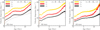 |
Fig. 4 Derived age-velocity dispersions for three different 2-kpc-wide annuli (the Sun is located at R⊙ = 8.249 kpc). The width of the lines corresponds to the statistical uncertainty on the dispersion
|
![Mathematical equation: $\[(\sigma / \sqrt{2(n-1)}\]$](/articles/aa/full_html/2025/11/aa56657-25/aa56657-25-eq1.png)
2.4 Age determination
The ages (τ) were computed using the Kordopatis et al. (2023b) pipeline, projecting on PARSEC isochrones (Bressan et al. 2012), the XGBoost Teff, log g, [M/H], as well as the extinction-corrected absolute magnitudes in the G, GBP, GRP, W1, and W2 bands. The de-reddening was done using the python code dustmaps (Green 2018), querying the Green et al. (2019) 3D map where available, or the Schlegel et al. (1998) map, corrected for the stellar distance as in Kordopatis et al. (2015b). We note that the maximum metallicity reached by the adopted PARSEC isochrones is +1.0 dex and maximum age is τ = 19.95 Gyr. From the resulting values, we filtered out the estimations when the age uncertainties were smaller than 0.1 Gyr (i.e. unrealistic uncertainties) or greater than 50% (potentially biased ages; see Kordopatis et al. 2023b). The relative age uncertainty distribution, for the filtered sample, peaks at 28%.
As a validation of our ages, we investigated the derived age-velocity dispersions (in the radial, azimuthal, and vertical directions, noted σR, σϕ, and σz, respectively) for three different 2-kpc-wide annuli, shown in Fig. 4. On top of the found trends, we plot the same power law of the form σV = β · τk as often done in the literature and defined in the solar neighbourhood (e.g. Wielen 1977; Casagrande et al. 2011, see however, Seabroke & Gilmore 2007; Martig et al. 2014 for discussions on why this may not be a sensible choice). We find that our trends can be split in three regimes, a rapid increase (up to 5 Gyr), a rather flat regime (between 5 and 9–10 Gyr) and a jump in the velocity dispersion for the older ages, where the thick disc and the halo start dominating. These are the typical trends expected in our Galaxy, as also found in other studies (see the review of Bland-Hawthorn & Gerhard 2016). One can also notice that the σR,ϕ,z trends decrease when moving towards larger radii. This will be further discussed in Sect. 3.1.
For the stars located at the solar annulus (middle plot of Fig. 4), our derived velocity dispersions for the youngest ages (≲1 Gyr) are larger than the exponential law and have a decreasing trend.3 This may be due to the accumulation of older stars with underestimated ages. This will be further discussed in the following sections. Nevertheless, for τ = 1.5 Gyr, we find (σR, σϕ, σz) ~ (25, 17, 12) km s−1; this is in agreement with the values found in the literature, which range between 20 and 30 km s−1 for σR, from 12 to 20 km s−1 for σϕ, and from 8 to 15 km s−1 for σz, (see e.g. Nordström et al. 2004; Soubiran et al. 2008; Casagrande et al. 2011; Mackereth et al. 2019; McCluskey et al. 2025).
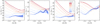 |
Fig. 5 Velocity dispersions (radial, azimuthal, and vertical in the first, second, and third panels) and average age (fourth panel) as a function of metallicity for different galactocentric guiding radii, Rg, as annotated by the legend. The ‘X’ symbols are located at the ISM’s metallicity at the considered position, assuming the metallicity gradient derived from classical Cepheids and open clusters from da Silva et al. (2023). The thickness of the line corresponds to the uncertainty on the measurement. The step in metallicity used to compute the trends is 0.1 dex. |
3 Velocity dispersions and age trends across the Galaxy
We next investigated the change in the mean age and velocity dispersions as a function of metallicity for different 1-kpc-wide annuli in the Galaxy. Results are shown in Fig. 5, where the position of the stars is based on their guiding radius. This minimises the effect of blurring since the mixing caused by stars on eccentric orbits is removed and hence the mean locus of the stars in the Galaxy is more accurately reflected. Figure B.1 shows the same plots as in Fig. 5, for a selection based on measured galactocentric radius, i.e. R. On top of each curve, we plot with an ‘×’ symbol, today’s ISM metallicity at the considered location, adopting the da Silva et al. 2023 metallicity log-gradient (see Sect. 1). The x-positions of the ‘×’ are therefore completely independent of any measurement done in this study (while the y-position is always our measurement). Stars with metallicities rightwards of this ‘×’ are therefore LMR.
3.1 Trends as a function of distance from the Galactic centre
We first focused on the velocity dispersion trends as a function of Rg, i.e. at a fixed metallicity. Figure 5 shows that, on average, the velocity dispersion for all three components drops, as one moves towards larger Galactic radii (different curves, from red to blue).
The separation between the velocity dispersion curves gets smaller with increasing Rg. This is particularly true for σz, for which the trend is in agreement with Gaia Collaboration (2018), Sanders & Das (2018), and Khoperskov et al. (2025), and is an additional validation of the adopted metallicities, positions and kinematics. The drop in the velocity dispersion as a function of Rg is expected for a disc in equilibrium, whose surface density, Σ(R), varies as ![Mathematical equation: $\[\sigma_{z}^{2} / h_{z}\]$](/articles/aa/full_html/2025/11/aa56657-25/aa56657-25-eq2.png) , with hz its scale-height (van der Kruit 1988). In other words, assuming that Σ(R) drops with R (e.g. McMillan 2017) and that hz is either constant or increases with R due to flaring (e.g. van der Kruit & Freeman 2011; Minchev et al. 2015), σZ has to decrease with R, as we see from our data too (see also Fig. 4).
, with hz its scale-height (van der Kruit 1988). In other words, assuming that Σ(R) drops with R (e.g. McMillan 2017) and that hz is either constant or increases with R due to flaring (e.g. van der Kruit & Freeman 2011; Minchev et al. 2015), σZ has to decrease with R, as we see from our data too (see also Fig. 4).
Regarding the ages, we find that the stars in the inner Galaxy are older than the stars in the outer Galaxy as long as we considered metallicities below the ones of the ISM. Again, this is the expected trend for a disc formed inside-out, as we believe was the case for the Milky Way (e.g. Fall & Efstathiou 1980; Mo et al. 1998; Frankel et al. 2019; Minchev et al. 2019). Above the ISM’s metallicity, the separation between the age curves of different Rg is more complex: not only do we find that the separation is tighter, but it also appears that the age gradient is reversed, i.e. at a fixed metallicity the stars at the outer radii are older, on average, than at the annuli of smaller Rg.
3.2 Trends as a function of metallicity
3.2.1 Below the ISM metallicity
We next investigated the velocity dispersion and mean age trends as a function of metallicity, i.e. at a fixed Rg. As mentioned in the previous section, we find, for all velocity components, a drop in σ as a function of [M/H], up to [M/H]ISM. Assuming that, to the zeroth order, there is an age-metallicity relation (as confirmed by the fourth plot of Fig. 5, showing an age decrease up to [M/H]ISM), the drop in σ as a function of [M/H] can therefore be associated with the well-known age-velocity dispersion relation in the disc (see Sect. 2.4). Stars with metallicities lower than the ISM (Δ[M/H]ISM < 0) are either stars born locally that had time to be dynamically heated or stars born at different locations that have been churned and/or blurred, and hence with older ages and hotter kinematics too, compared to locally born stars.
Focusing on Rg ~ R⊙ (grey curve), we find that the velocity dispersion of the stars that have the same metallicity as the ISM is σZ ~ 16 km s−1. This is consistent with the literature values of, for example, Nordström et al. (2004), Casagrande et al. (2011), and Mackereth et al. (2019) for τ ~ 5 Gyr stars, which is also the average age we get from the fourth panel of Fig. 5.
One could have a priori expected a lower age and a lower velocity dispersion at Rg = R⊙ and [M/H]=[M/H]ISM since the solar neighbourhood only now reaches solar metallicities for newborn stars (e.g. Ritchey et al. 2023). There are at least three factors that can contribute to such high values in our study:
(a) A selection bias in our sample against the youngest stars. This point is certainly true. Indeed, no bright massive stars are within the magnitude limits (all stars are fainter than G ~ 9) and, in addition, the XGBoost catalogue we used is limited to RGB stars. Therefore, young stars are under-represented in the sample, which implies a higher average age in the solar neighbourhood and hence a higher velocity dispersion. This is indeed what we find qualitatively.
(b) A bias due to the effect of age and metallicity uncertainties. This second point whereas it is true, is not enough to explain the values that we derived. Indeed, Fig. 4 indicates that we do not properly recover the expected velocity dispersion for τ = 0.5 Gyr stars (~14 km s−1 instead of ~10 km s−1). However, since metallicity uncertainties are expected to be of the order of ~0.1 dex (Andrae et al. 2023), this naturally shifts some metal-poorer stars (and hence older, on average) into higher metallicity bins, inflating that way the velocity dispersion. Appendix C discusses the effect attributed to a contamination from older and lower-metallicity stars being part of the high-end tail of the metallicity error distribution, and concludes that if one assumes the reported uncertainties of Andrae et al. (2023) as true, then such a contamination cannot explain by itself the large dispersion.
(c) The presence of a significant amount of intrinsically old solar metallicity stars in the solar neighbourhood. This is also likely true. Several observations of solar-metallicity field stars, with ages determined by different methods corroborate that such stars exist (e.g. Bensby et al. 2014; Kordopatis et al. 2015b; Gondoin 2023; Lehmann et al. 2024; Nepal et al. 2024), whereas the Sun itself is older than 4.5 Gyr (e.g. Bahcall et al. 1995; Bouvier & Wadhwa 2010; Connelly et al. 2012) and is thought to have migrated by 2–3 kpc from its birthplace (e.g. Nieva & Przybilla 2012; Baba et al. 2023).
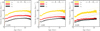 |
Fig. 6 Derived age-velocity dispersions for three different 2-kpc-wide annuli (the Sun is located at Rsol = 8.249 kpc) for LMR stars, i.e. stars that are more metal-rich than the ISM’s metallicity at their guiding radius, with Δ[M/H]ISM > 0.1. The colours and the dashed lines are same as in Fig. 4. |
3.2.2 Above the ISM metallicity
For LMR stars, the drop in velocity dispersions as a function of [M/H], seen for lower metallicities, stops. That is, the LMR stars have velocity dispersions in all three components rather flat as a function of metallicity, marginally higher than the presently locally born stars. This is true for all the considered metallicities above the local ISM, up to Δ[M/H]ISM ~ +0.5 dex. Indeed, as also shown in Fig. 6, the velocity dispersions of the LMR stars, as a function of age is much flatter than the trends found when considering all of the stars (see Fig. 4).
This trend is global in the disc, and does not depend on the azimuth. This is best shown in the last two rows of Fig. 7, which illustrates, in the X − Y plane, the σZ ratio between stars of different Δ[M/H]ISM ranges. In this figure, a clear dichotomy can be noticed for R ~ 8–10 kpc. Beyond that radius, LMR stars of a given Δ[M/H]ISM have larger velocity dispersion than stars with metallicities down to 0.2 dex below the local ISM (blue colour), whereas this trend reverses at R ~ R⊙. Using the photometric [α/M] of Li et al. (2024b), we find no clear evidence that this dichotomy can be due to an ‘edge’ of the high-α disc (which has a larger velocity dispersion), and in particular its absence at large radii (e.g. Bensby et al. 2011; Kordopatis et al. 2015a; Hayden et al. 2015). Relative to the location of the resonances in the disc, this distance, is beyond the bar’s co-rotation radius (~6.5–7.5 kpc, assuming a pattern speed of Ωb ≈ 35–40 km s−1 kpc−1; e.g. Chiba et al. 2021; Clarke & Gerhard 2022; Gaia Collaboration 2023a; Zhang et al. 2024)4 and smaller than its outer Lindblad resonance (ROLR of ~10.7–12.4 kpc) but compatible with the m = 4, higher order outer Lindblad resonance of ~8.7–10.0 kpc (Clarke & Gerhard 2022).
Finally, regarding the age-trends, the right-most panel of Fig. 5 shows a clear uprise of the average age for stars with Δ[M/H]ISM > 0. This rules out Galactic fountains as the main mechanism forming the LMR star, as one would expect either a flatter trend (in the case of short radial mixing) or a decrease in the age as a function of metallicity (in the case of large radial mixing; Grand et al. 2019). This rise is, in fact, illustrating that LMR stars need time to migrate and reach their position. Furthermore, we find that for all the investigated annuli (except the innermost one) the increase in mean age as a function of metallicity follows a similar trend. This is indicative of the fact that radial migration is as effective at all the probed radii, hinting towards having the same mechanism causing their churning.
Another illustration of this can be seen in Fig. 8, which shows the X–Y distribution for stars of different Δ[M/H]ISM, colour-coded by density, mean eccentricity and mean age, for two different ranges of Zmax. The last two columns of Fig. 8 show clearly, from top to bottom, how we transit from a Galaxy where the inner parts are old and the outer young (first two rows, |Δ[M/H]ISM| < 0.1) to a Galaxy where all of the stars are old (Δ[M/H]ISM > 0.1). Similarly, the larger the Δ[M/H]ISM, the older the stars, as they have likely travelled farther, and needed time to reach their position.
4 Effect of the spiral arms across the disc on the LMR stars
Figures 7 and 8 allow us to better comprehend the trends we find with respect to the spiral arms and the central bar.
We started with the fact that old LMR stars are found at least up to 11 kpc from the Galactic centre, i.e. far beyond present day bar’s corotation radius (see Sect. 3.2.2). Since these stars are mostly on circular orbits (e ≲ 0.15; see Columns 2 and 3 of Fig. 8), i.e. they are not visitors on eccentric orbits, we can conclude that the bar alone cannot have shuffled them, and that co-rotation resonances with multiple spiral arms (and potentially overlapping spiral patterns with the bar; see Marques et al. 2025) need to come into play.
One can also conclude that, at least up to R ~ R⊙, churned stars do not significantly heat the disc, confirming to some extent the N-body simulation findings of Minchev et al. (2012) and Halle et al. (2015), as well as the results obtained with the forward-modelling of Frankel et al. (2020). This conclusion, however, needs to be taken with a grain of salt. Figure 7 shows that, farther than R⊙, the LMR stars consistently have a velocity dispersion slightly greater (~20%) than stars with a metallicity equal to the ISM’s. This trend does not seem to be related to the absence of α-high stars (i.e. thick disc stars) at large radii and cannot be entirely explained by errors in velocity and/or metallicities. This increase, however, may be indicative of the relative quiescent merger history of the Milky Way. Minchev et al. (2012) have shown that the velocity dispersion decay of migrators ending up at a given radius (R) can be expressed as σz,mig(R) ~ exp(−R/4Rd), which is two times slower than the one of the non-migrating disc stars (σz(R) ~ exp (−R/2Rd)). However, migrating stars usually still end up, with cooler kinematics than local populations due to a provenance bias (i.e. only dynamically cool stars who spend time in the plane migrate preferentially; see Vera-Ciro et al. 2014) and/or due to the heating of locally born stars by merger interactions (Martig et al. 2014). The fact that we find the LMR stars at R >R⊙ with slightly warmer kinematics therefore seems to indicate that the mergers that happened over the last 10 Gyr of the history of the Milky Way have not heated the disc significantly enough, because they were too few and/or not massive enough (Deason & Belokurov 2024, and references therein).
Furthermore, the trend that we measure does not seem to have an azimuthal dependence. This implies that if it is the resonances with the arms that brought the LMR stars where they are, then their non-axisymmetric effects are smoothed out rapidly.
However, we find that the actual presence of the spiral arms does affect, locally, the average eccentricity and age of the LMR stars. Based on Fig. 8, where the spiral arms are plotted in light-grey, as estimated by Castro-Ginard et al. (2021), one can see that:
(a) The presence of LMR stars does not coincide with over-densities at the location of the spiral arms (Column 1). This is consistent with the spirals being a density wave (Lin & Shu 1964) rather than material winding spirals (e.g. Toomre 1981; Grand et al. 2012).
(b) LMR stars located at the position of the spiral arms tend to have lower eccentricities (blue stripes in Columns 2 and 3 of Fig. 8). The effect of the presence of spirals is seen up to Zmax ~ 0.5 kpc5 and up to metallicities more than 0.4 dex higher than the ISM. This is in agreement with Debattista et al. (2025); Palicio et al. (2025) who found that there is a spatial correlation between spiral arms and stellar populations featuring low values of the radial action, and with Martinez-Medina et al. (2025) who found the spiral arms extending up to 400 pc from the plane.
(c) LMR stars located at the position of the spiral arms also show hints of being slightly younger than LMR stars located in between the arms with the same Δ[M/H]ISM. This is better visualised in the last two rows, both close to and far from the plane, but the uncertainties in the derived ages imply that a more thorough analysis (with, if possible, even smaller age-uncertainties) needs to be conducted to confirm this point.
 |
Fig. 7 X − Y maps showing the ratio of the vertical velocity dispersion of stars at a given metallicity range to the ISM’s value (rightmost panel of each row, with the σz map in grey), and stars with a lower metal content, in bins of 0.1 dex(σZ,n, remaining panels). Over-plotted in grey lines are the spiral arm locations, as estimated by Castro-Ginard et al. (2021). Redder (bluer) colours indicate that the lower-metallicity stars have hotter (cooler) kinematics in the considered pixel. The assumed location of the Sun is indicated by a ‘+’ sign. Pixels are 0.5-kpc-wide and considered only if they include more than 200 stars in either selection. Stars with Zmax > 2 kpc have been discarded. One can see that at the outermost radii, stars that are considerably more metal-rich than the ISM tend to be slightly kinematically hotter than more metal-poor stars. |
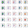 |
Fig. 8 X–Y maps of stars of different metallicities compared to the ISM’s one. Over-plotted in grey lines are the spiral arm locations, as estimated by Castro-Ginard et al. (2021). The colour codes are as follows: density for all selected stars with Zmax< 0.25 kpc (column 1), eccentricity for the stars with a maximum orbital distance from the plane (Zmax) of 0.25 kpc (column 2), eccentricity for stars with Zmax between 0.25 and 0.5 kpc (Column 3), and ages of the stars from columns 2 and 3 (Columns 4 and 5). The age colour bar for the last row has a different range (from 5 to 9 Gyr) to better reflect the older ages, on average, of the extreme LMR stars. |
5 Conclusions and perspectives
In this study, we conducted a kinematic and age analysis of the LMR stars, i.e. stars whose metallicities exceed that of the ISM at their guiding radius. Leveraging Gaia photometric metallicities, we identified and analysed millions of such stars across the Galactic disc. Our main findings are as follows:
LMR stars are consistently older than locally born stars whose metallicities match that of the ISM, yet their velocity dispersions are only slightly higher, confirming that radial migration does not significantly heat the disc – a key theoretical prediction now supported by observations without modelling;
At a fixed metallicity excess relative to the ISM, LMR stars located farther out in the disc are systematically older, indicating a time-dependent outward migration consistent with an inside-out growth of the disc and a gradual migration on gigayear timescales;
No correlation is found between spiral arm locations and the density of LMR stars, but the mean stellar eccentricity and age show minima near spiral structures, confirming a kinematic and temporal influence of spiral arms on migrating populations;
The age distribution of LMR stars is inconsistent with a Galactic fountain origin, providing strong evidence in favour of radial migration rather than ejection–re-accretion mechanisms;
While we do not detect any clear spatial signatures uniquely attributable to the Galactic bar, this does not preclude its influence. As bar-induced migration is expected to be phase-mixed and act over large spatial scales, particularly near resonances like the outer Lindblad resonance, its dynamical effects may not leave obvious azimuthal or spatial imprints in the LMR population. Furthermore, interactions between the bar and spiral arms can generate complex patterns that may be difficult to isolate without detailed dynamical modelling.
These results pave the way for more detailed future work. Upcoming large-scale spectroscopic surveys such as 4MOST (de Jong et al. 2019) and WEAVE (Jin et al. 2024) will deliver more accurate metallicities, stellar ages, and individual elemental abundances. These data will enable refined comparisons with chemical evolution models. Using models such as those of Kordopatis et al. (2015a) and Minchev et al. (2018), combined with individual elemental abundances tracing different nucleosynthetic channels, it will be possible to place constraints on the birth radii of these stars and to quantify the migration rate as a function of height above the Galactic plane.
Acknowledgements
We thank the anonymous referee for their comments and suggestions that helped improving the clarity of the paper. GK and VH gratefully acknowledge support from the French national research agency (ANR) funded project MWDisc (ANR-20-CE31-0004). SF, DF, CL and HE were supported by a project grant from the Knut and Alice Wallenberg Foundation (KAW 2020.0061 Galactic Time Machine, P.I. Feltzing). This project was supported by funds from the Crafoord foundation (reference 20230890). IM acknowledges support by the Deutsche Forschungsgemeinschaft under the grant MI 2009/2-1. DF acknowledges funding from the Swedish Research Council grant 2022-03274. Gregor Traven is thanked for the useful plotting tips he gave. Apolline Kordopatis is also thanked for having been a very quiet newborn baby, and Vanessa Gardet for having been an amazing mom during the first weeks of Apolline in this world; both of them were of an immense help to finalise this paper. This work has made use of data from the European Space Agency (ESA) mission Gaia (https://www.cosmos.esa.int/gaia), processed by the Gaia Data Processing and Analysis Consortium (DPAC, https://www.cosmos.esa.int/web/gaia/dpac/consortium). Funding for the DPAC has been provided by national institutions, in particular the institutions participating in the Gaia Multilateral Agreement. This research made use of Astropy (http://www.astropy.org) a community-developed core Python package for Astronomy (Astropy Collaboration 2013; Price-Whelan et al. 2018).
Appendix A Effect of the different cuts on the metallicity distributions
Figure A.1 shows in grey the metallicity distribution between −1.3 and +0.5 of the XGBoost RGB sample, cross-matched with the AspGap one for all of the stars (11 · 106 stars, top) and the LMR ones (2.82 · 106, bottom). The effect on the distribution due to the successive filtering on the RUWE parameter (in blue), the parallax uncertainty (σϖ/ϖ, in green), the agreement between the AspGap and XGBoost metallicity (Δ[M/H]ISM, in yellow) and the Teff cut (in red) are also shown (see Sects. 2.1 and 2.2). We note that the parallax uncertainty cut removes most of the spurious XGBoost peak at [M/H] = 0. Eventually, once all the cuts applied, ~ 6.36 · 106 stars are left, among which 1.91 · 106 LMR. This sample drops to ~ 6.25 · 106 and ~ 1.86 · 106 once the filter on the age uncertainty is applied (light pink histogram; see Sect. 2.4).
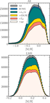 |
Fig. A.1 Metallicity distribution for the entire RGB sample (top) and the LMR subsample (bottom) once the successive quality filters have been applied (see Sects. 2.1, 2.2, and 2.4). |
Appendix B Velocity dispersion at different galactocentric radii
Figure B.1 is similar to Fig. 5, but the bins are in actual Galactic radius, R, rather than guiding radius, Rg. Similar velocity dispersion trends as the ones obtained using Rg cuts are found here as well, albeit smoothed out, due to the fact that each R bin can contain stars belonging to other annuli (due to blurring).
 |
Fig. B.1 Similar to Fig. 5 except that now the position of the stars within an annulus is determined by their actual R position, instead of Rg. When plotting as a function of R, stars are preferentially seen at their apocentre and, therefore, on cooler orbits. |
Appendix C Estimation of the contamination from lower-metallicity and older stars
In Sect. 3.2 and Fig. 5, we find that [M/H] ~ 0 stars at Rg ~ R⊙ have a vertical velocity dispersion ~ 5 km s−1 larger than what found from previous spectroscopic studies. Since kinematic measurements are expected to be very precise because they are based on Gaia data of relatively nearby stars, one can use this value to estimate qualitatively the amount of contamination from older and metal-poorer stars to the considered sample, and see if this contamination is greater than the one expected from the metallicity uncertainties alone.
Let us consider two populations A and B. Population A has a solar metallicity and an age τ = 0 Gyr, and population B has [M/H] = −0.1 (i.e. corresponding to the metallicity uncertainty estimated by Andrae et al. 2023). Following the age-metallicity relation of, for example, Spitoni et al. (2019), based on the asteroseismic ages of Silva Aguirre et al. (2018), stars with [M/H] = −0.1 dex can be as old as 5 Gyr. Adopting an age-velocity dispersion relation in the form σz = a · τk with a = 10 km s−1 and k = 0.47 (e.g. Kordopatis et al. 2015a), this results to σz,B = 21 km s−1.
The combined velocity dispersion, σcombined, of the two populations, is then defined as ![Mathematical equation: $\[\sigma_{\text {combined }}^{2}=x \cdot \sigma_{A}^{2}+(1-x) \cdot \sigma_{B}^{2}\]$](/articles/aa/full_html/2025/11/aa56657-25/aa56657-25-eq3.png) with x the proportion of population A, and σA and σB are the respective velocity dispersions of each population. Since the measured vertical velocity dispersion at τ ~ 0.5 Gyr in Fig. 4 is 14 km s−1, one can conclude that x = 0.75 and that therefore the contamination of metal-poorer stars is of the order of 25 per cent. This value is therefore above the ~ 16 per cent contamination expected from a unit gaussian centred at [M/H] = −0.1 with a standard deviation of 0.1.
with x the proportion of population A, and σA and σB are the respective velocity dispersions of each population. Since the measured vertical velocity dispersion at τ ~ 0.5 Gyr in Fig. 4 is 14 km s−1, one can conclude that x = 0.75 and that therefore the contamination of metal-poorer stars is of the order of 25 per cent. This value is therefore above the ~ 16 per cent contamination expected from a unit gaussian centred at [M/H] = −0.1 with a standard deviation of 0.1.
We conclude that, to explain the large velocity dispersion we obtain, one has to assume either that the reported XGBoost uncertainties are underestimated or that the sample is biased against young stars and/or contains intrinsically older stars (see the discussion in Sect 3.2).
References
- Abdurro’uf, Accetta, K., Aerts, C., et al. 2022, ApJS, 259, 35 [NASA ADS] [CrossRef] [Google Scholar]
- Andrae, R., Rix, H.-W., & Chandra, V. 2023, ApJS, 267, 8 [NASA ADS] [CrossRef] [Google Scholar]
- Astropy Collaboration (Robitaille, T. P., et al.) 2013, A&A, 558, A33 [NASA ADS] [CrossRef] [EDP Sciences] [Google Scholar]
- Baba, J., Saitoh, T. R., & Tsujimoto, T. 2023, MNRAS, 526, 6088 [Google Scholar]
- Bahcall, J. N., Pinsonneault, M. H., & Wasserburg, G. J. 1995, Rev. Mod. Phys., 67, 781 [Google Scholar]
- Bailer-Jones, C. A. L., Rybizki, J., Fouesneau, M., Demleitner, M., & Andrae, R. 2021, AJ, 161, 147 [Google Scholar]
- Bennett, M., & Bovy, J. 2019, MNRAS, 482, 1417 [NASA ADS] [CrossRef] [Google Scholar]
- Bensby, T., Alves-Brito, A., Oey, M. S., Yong, D., & Meléndez, J. 2011, ApJ, 735, L46 [NASA ADS] [CrossRef] [Google Scholar]
- Bensby, T., Feltzing, S., & Oey, M. S. 2014, A&A, 562, A71 [NASA ADS] [CrossRef] [EDP Sciences] [Google Scholar]
- Bland-Hawthorn, J., & Gerhard, O. 2016, ARA&A, 54, 529 [Google Scholar]
- Bouvier, A., & Wadhwa, M. 2010, Nat. Geosci., 3, 637 [NASA ADS] [CrossRef] [Google Scholar]
- Bressan, A., Marigo, P., Girardi, L., et al. 2012, MNRAS, 427, 127 [NASA ADS] [CrossRef] [Google Scholar]
- Buder, S., Kos, J., Wang, X. E., et al. 2025, PASA, 42, e051 [Google Scholar]
- Casagrande, L., Schönrich, R., Asplund, M., et al. 2011, A&A, 530, A138 [NASA ADS] [CrossRef] [EDP Sciences] [Google Scholar]
- Castro-Ginard, A., McMillan, P. J., Luri, X., et al. 2021, A&A, 652, A162 [NASA ADS] [CrossRef] [EDP Sciences] [Google Scholar]
- Chiba, R., Friske, J. K. S., & Schönrich, R. 2021, MNRAS, 500, 4710 [Google Scholar]
- Clarke, J. P., & Gerhard, O. 2022, MNRAS, 512, 2171 [NASA ADS] [CrossRef] [Google Scholar]
- Connelly, J. N., Bizzarro, M., Krot, A. N., et al. 2012, Science, 338, 651 [Google Scholar]
- da Silva, R., D’Orazi, V., Palla, M., et al. 2023, A&A, 678, A195 [NASA ADS] [CrossRef] [EDP Sciences] [Google Scholar]
- Daniel, K. J., Schaffner, D. A., McCluskey, F., Fiedler Kawaguchi, C., & Loebman, S. 2019, ApJ, 882, 111 [NASA ADS] [CrossRef] [Google Scholar]
- Dantas, M. L. L., Smiljanic, R., Boesso, R., et al. 2023, A&A, 669, A96 [NASA ADS] [CrossRef] [EDP Sciences] [Google Scholar]
- de Jong, R. S., Agertz, O., Berbel, A. A., et al. 2019, The Messenger, 175, 3 [NASA ADS] [Google Scholar]
- Deason, A. J., & Belokurov, V. 2024, New Astron. Rev., 99, 101706 [CrossRef] [Google Scholar]
- Debattista, V. P., Khachaturyants, T., Amarante, J. A. S., et al. 2025, MNRAS, 537, 1620 [Google Scholar]
- Di Matteo, P., Haywood, M., Combes, F., Semelin, B., & Snaith, O. N. 2013, A&A, 553, A102 [NASA ADS] [CrossRef] [EDP Sciences] [Google Scholar]
- Fall, S. M., & Efstathiou, G. 1980, MNRAS, 193, 189 [NASA ADS] [CrossRef] [Google Scholar]
- Frankel, N., Sanders, J., Rix, H.-W., Ting, Y.-S., & Ness, M. 2019, ApJ, 884, 99 [Google Scholar]
- Frankel, N., Sanders, J., Ting, Y.-S., & Rix, H.-W. 2020, ApJ, 896, 15 [NASA ADS] [CrossRef] [Google Scholar]
- Fraternali, F., Marasco, A., Marinacci, F., & Binney, J. 2013, ApJ, 764, L21 [Google Scholar]
- Gaia Collaboration (Prusti, T., et al.) 2016, A&A, 595, A1 [NASA ADS] [CrossRef] [EDP Sciences] [Google Scholar]
- Gaia Collaboration (Katz, D., et al.) 2018, A&A, 616, A11 [NASA ADS] [CrossRef] [EDP Sciences] [Google Scholar]
- Gaia Collaboration (Drimmel, R., et al.) 2023a, A&A, 674, A37 [CrossRef] [EDP Sciences] [Google Scholar]
- Gaia Collaboration (Recio-Blanco, A., et al.) 2023b, A&A, 674, A38 [CrossRef] [EDP Sciences] [Google Scholar]
- Gaia Collaboration (Vallenari, A., et al.) 2023c, A&A, 674, A1 [NASA ADS] [CrossRef] [EDP Sciences] [Google Scholar]
- Genovali, K., Lemasle, B., Bono, G., et al. 2014, A&A, 566, A37 [NASA ADS] [CrossRef] [EDP Sciences] [Google Scholar]
- Gómez, F. A., Minchev, I., O’Shea, B. W., et al. 2013, MNRAS, 429, 159 [Google Scholar]
- Gondoin, P. 2023, A&A, 678, A39 [NASA ADS] [CrossRef] [EDP Sciences] [Google Scholar]
- Grand, R. J. J., Kawata, D., & Cropper, M. 2012, MNRAS, 426, 167 [NASA ADS] [CrossRef] [Google Scholar]
- Grand, R. J. J., van de Voort, F., Zjupa, J., et al. 2019, MNRAS, 490, 4786 [Google Scholar]
- GRAVITY Collaboration (Abuter, R., et al.) 2020, A&A, 636, L5 [NASA ADS] [CrossRef] [EDP Sciences] [Google Scholar]
- Green, G. 2018, J. Open Source Softw., 3, 695 [NASA ADS] [CrossRef] [Google Scholar]
- Green, G. M., Schlafly, E., Zucker, C., Speagle, J. S., & Finkbeiner, D. 2019, ApJ, 887, 93 [NASA ADS] [CrossRef] [Google Scholar]
- Grenon, M. 1972, in IAU Colloq. 17: Age des Etoiles, eds. G. Cayrel de Strobel, & A. M. Delplace, 55 [Google Scholar]
- Halle, A., Di Matteo, P., Haywood, M., & Combes, F. 2015, A&A, 578, A58 [NASA ADS] [CrossRef] [EDP Sciences] [Google Scholar]
- Hamilton, C., Modak, S., & Tremaine, S. 2024, arXiv e-prints [arXiv:2411.08944] [Google Scholar]
- Hattori, K. 2024, arXiv e-prints [arXiv:2404.01269] [Google Scholar]
- Hayden, M. R., Bovy, J., Holtzman, J. A., et al. 2015, ApJ, 808, 132 [Google Scholar]
- Haywood, M., Khoperskov, S., Cerqui, V., et al. 2024, A&A, 690, A147 [NASA ADS] [CrossRef] [EDP Sciences] [Google Scholar]
- Hilmi, T., Minchev, I., Buck, T., et al. 2020, MNRAS, 497, 933 [Google Scholar]
- Ida, S., Kokubo, E., & Makino, J. 1993, MNRAS, 263, 875 [Google Scholar]
- Jin, S., Trager, S. C., Dalton, G. B., et al. 2024, MNRAS, 530, 2688 [NASA ADS] [CrossRef] [Google Scholar]
- Katz, D., Sartoretti, P., Guerrier, A., et al. 2023, A&A, 674, A5 [NASA ADS] [CrossRef] [EDP Sciences] [Google Scholar]
- Kazantzidis, S., Bullock, J. S., Zentner, A. R., Kravtsov, A. V., & Moustakas, L. A. 2008, ApJ, 688, 254 [Google Scholar]
- Khoperskov, S., Di Matteo, P., Haywood, M., Gómez, A., & Snaith, O. N. 2020, A&A, 638, A144 [NASA ADS] [CrossRef] [EDP Sciences] [Google Scholar]
- Khoperskov, S., & Gerhard, O. 2022, A&A, 663, A38 [NASA ADS] [CrossRef] [EDP Sciences] [Google Scholar]
- Khoperskov, S., Steinmetz, M., Haywood, M., et al. 2025, A&A, 700, A89 [NASA ADS] [CrossRef] [EDP Sciences] [Google Scholar]
- Kordopatis, G., Recio-Blanco, A., de Laverny, P., et al. 2011, A&A, 535, A106 [NASA ADS] [CrossRef] [EDP Sciences] [Google Scholar]
- Kordopatis, G., Gilmore, G., Steinmetz, M., et al. 2013, AJ, 146, 134 [Google Scholar]
- Kordopatis, G., Binney, J., Gilmore, G., et al. 2015a, MNRAS, 447, 3526 [Google Scholar]
- Kordopatis, G., Wyse, R. F. G., Gilmore, G., et al. 2015b, A&A, 582, A122 [NASA ADS] [CrossRef] [EDP Sciences] [Google Scholar]
- Kordopatis, G., Recio-Blanco, A., Schultheis, M., & Hill, V. 2020, A&A, 643, A69 [NASA ADS] [CrossRef] [EDP Sciences] [Google Scholar]
- Kordopatis, G., Hill, V., & Lind, K. 2023a, A&A, 674, A104 [NASA ADS] [CrossRef] [EDP Sciences] [Google Scholar]
- Kordopatis, G., Schultheis, M., McMillan, P. J., et al. 2023b, A&A, 669, A104 [NASA ADS] [CrossRef] [EDP Sciences] [Google Scholar]
- Kos, J., Buder, S., Beeson, K. L., et al. 2025, arXiv e-prints [arXiv:2501.06140] [Google Scholar]
- Lacey, C. G. 1984, MNRAS, 208, 687 [NASA ADS] [CrossRef] [Google Scholar]
- Laporte, C. F. P., Koposov, S. E., & Belokurov, V. 2022, MNRAS, 510, L13 [Google Scholar]
- Lehmann, C., Feltzing, S., Feuillet, D., & Kordopatis, G. 2024, MNRAS, 533, 538 [NASA ADS] [CrossRef] [Google Scholar]
- Li, H., Aoki, W., Matsuno, T., et al. 2022, ApJ, 931, 147 [NASA ADS] [CrossRef] [Google Scholar]
- Li, C., Siebert, A., Monari, G., Famaey, B., & Rozier, S. 2023, MNRAS, 524, 6331 [NASA ADS] [CrossRef] [Google Scholar]
- Li, C., Yuan, Z., Monari, G., et al. 2024a, A&A, 690, A26 [NASA ADS] [CrossRef] [EDP Sciences] [Google Scholar]
- Li, J., Wong, K. W. K., Hogg, D. W., Rix, H.-W., & Chandra, V. 2024b, ApJS, 272, 2 [NASA ADS] [CrossRef] [Google Scholar]
- Lian, J., Zasowski, G., Hasselquist, S., et al. 2022, MNRAS, 511, 5639 [NASA ADS] [CrossRef] [Google Scholar]
- Lin, C. C., & Shu, F. H. 1964, ApJ, 140, 646 [Google Scholar]
- Lindegren, L. 2018, gAIA-C3-TN-LU-LL-124 [Google Scholar]
- Lu, Y. L., Minchev, I., Buck, T., et al. 2024, MNRAS, 535, 392 [NASA ADS] [CrossRef] [Google Scholar]
- Lynden-Bell, D., & Kalnajs, A. J. 1972, MNRAS, 157, 1 [Google Scholar]
- Mackereth, J. T., Bovy, J., Leung, H. W., et al. 2019, MNRAS, 489, 176 [Google Scholar]
- Marques, L., Minchev, I., Ratcliffe, B., et al. 2025, A&A, 701, A88 [NASA ADS] [CrossRef] [EDP Sciences] [Google Scholar]
- Martig, M., Minchev, I., & Flynn, C. 2014, MNRAS, 443, 2452 [Google Scholar]
- Martin, N. F., Starkenburg, E., Yuan, Z., et al. 2024, A&A, 692, A115 [NASA ADS] [CrossRef] [EDP Sciences] [Google Scholar]
- Martinez-Medina, L., Poggio, E., & Moreno-Hilario, E. 2025, MNRAS, 542, L94 [Google Scholar]
- McCluskey, F., Wetzel, A., Loebman, S., & Moreno, J. 2025, arXiv e-prints [arXiv:2506.11840] [Google Scholar]
- McMillan, P. J. 2017, MNRAS, 465, 76 [NASA ADS] [CrossRef] [Google Scholar]
- Minchev, I., & Famaey, B. 2010, ApJ, 722, 112 [Google Scholar]
- Minchev, I., & Quillen, A. C. 2006, MNRAS, 368, 623 [NASA ADS] [CrossRef] [Google Scholar]
- Minchev, I., Famaey, B., Quillen, A. C., et al. 2012, A&A, 548, A127 [NASA ADS] [CrossRef] [EDP Sciences] [Google Scholar]
- Minchev, I., Martig, M., Streich, D., et al. 2015, ApJ, 804, L9 [NASA ADS] [CrossRef] [Google Scholar]
- Minchev, I., Anders, F., Recio-Blanco, A., et al. 2018, MNRAS, 481, 1645 [NASA ADS] [CrossRef] [Google Scholar]
- Minchev, I., Matijevic, G., Hogg, D. W., et al. 2019, MNRAS, 487, 3946 [NASA ADS] [Google Scholar]
- Mo, H. J., Mao, S., & White, S. D. M. 1998, MNRAS, 295, 319 [Google Scholar]
- Nepal, S., Chiappini, C., Guiglion, G., et al. 2024, A&A, 681, L8 [NASA ADS] [CrossRef] [EDP Sciences] [Google Scholar]
- Nieva, M.-F., & Przybilla, N. 2012, A&A, 539, A143 [NASA ADS] [CrossRef] [EDP Sciences] [Google Scholar]
- Nordström, B., Mayor, M., Andersen, J., et al. 2004, A&A, 418, 989 [Google Scholar]
- Palicio, P. A., Recio-Blanco, A., Tepper-García, T., et al. 2025, A&A, 695, A193 [NASA ADS] [CrossRef] [EDP Sciences] [Google Scholar]
- Price-Whelan, A. M., Sipőcz, B. M., Günther, H. M., et al. 2018, AJ, 156, 123 [NASA ADS] [CrossRef] [Google Scholar]
- Quillen, A. C. 2003, AJ, 125, 785 [NASA ADS] [CrossRef] [Google Scholar]
- Ratcliffe, B., Minchev, I., Anders, F., et al. 2023, MNRAS, 525, 2208 [NASA ADS] [CrossRef] [Google Scholar]
- Reid, M. J., & Brunthaler, A. 2020, ApJ, 892, 39 [Google Scholar]
- Ritchey, A. M., Jenkins, E. B., Shull, J. M., et al. 2023, ApJ, 952, 57 [NASA ADS] [CrossRef] [Google Scholar]
- Sanders, J. L., & Das, P. 2018, MNRAS, 481, 4093 [CrossRef] [Google Scholar]
- Santos-Peral, P., Recio-Blanco, A., Kordopatis, G., Fernández-Alvar, E., & de Laverny, P. 2021, A&A, 653, A85 [NASA ADS] [CrossRef] [EDP Sciences] [Google Scholar]
- Schlegel, D. J., Finkbeiner, D. P., & Davis, M. 1998, ApJ, 500, 525 [Google Scholar]
- Schönrich, R., & Binney, J. 2009, MNRAS, 399, 1145 [Google Scholar]
- Schönrich, R., Binney, J., & Dehnen, W. 2010, MNRAS, 403, 1829 [NASA ADS] [CrossRef] [Google Scholar]
- Seabroke, G. M., & Gilmore, G. 2007, MNRAS, 380, 1348 [NASA ADS] [CrossRef] [Google Scholar]
- Sellwood, J. A., & Binney, J. J. 2002, MNRAS, 336, 785 [Google Scholar]
- Sellwood, J. A., & Binney, J. 2025, arXiv e-prints [arXiv:2501.17907] [Google Scholar]
- Sellwood, J. A., & Masters, K. L. 2022, ARA&A, 60, 73 [NASA ADS] [CrossRef] [Google Scholar]
- Sharma, S., Hayden, M. R., Bland-Hawthorn, J., et al. 2021, MNRAS, 506, 1761 [NASA ADS] [CrossRef] [Google Scholar]
- Silva Aguirre, V., Bojsen-Hansen, M., Slumstrup, D., et al. 2018, MNRAS, 475, 5487 [NASA ADS] [Google Scholar]
- Soubiran, C., Bienaymé, O., Mishenina, T. V., & Kovtyukh, V. V. 2008, A&A, 480, 91 [NASA ADS] [CrossRef] [EDP Sciences] [Google Scholar]
- Spitoni, E., Silva Aguirre, V., Matteucci, F., Calura, F., & Grisoni, V. 2019, A&A, 623, A60 [NASA ADS] [CrossRef] [EDP Sciences] [Google Scholar]
- Spitzer, Jr., L., & Schwarzschild, M. 1951, ApJ, 114, 385 [NASA ADS] [CrossRef] [Google Scholar]
- Spitzer, Jr., L., & Schwarzschild, M. 1953, ApJ, 118, 106 [NASA ADS] [CrossRef] [Google Scholar]
- Toomre, A. 1981, in Structure and Evolution of Normal Galaxies, eds. S. M. Fall, & D. Lynden-Bell, 111 [Google Scholar]
- van der Kruit, P. C. 1988, A&A, 192, 117 [NASA ADS] [Google Scholar]
- van der Kruit, P. C., & Freeman, K. C. 2011, ARA&A, 49, 301 [Google Scholar]
- Velazquez, H., & White, S. D. M. 1999, MNRAS, 304, 254 [NASA ADS] [CrossRef] [Google Scholar]
- Vera-Ciro, C., D’Onghia, E., Navarro, J., & Abadi, M. 2014, ApJ, 794, 173 [NASA ADS] [CrossRef] [Google Scholar]
- Wielen, R. 1977, A&A, 60, 263 [NASA ADS] [Google Scholar]
- Zhang, H., Belokurov, V., Evans, N. W., et al. 2024, MNRAS, 535, 2873 [Google Scholar]
Stricter cuts were explored, without changing the results of the paper.
The suggested filtering flag_sp==0 has been applied.
The decrease in the velocity dispersions for the first gigayear in the solar annulus (middle panel of Fig. 4) is not found when we limit the sample to the extended solar neighbourhood, i.e. a bubble with a radius <1 kpc centred on the Sun.
Or even farther, if the pattern speed measured today is the maximum of a fluctuation Ωb, e.g. Hilmi et al. (2020); Li et al. (2023). In that case corotation may be even as small as 5 kpc.
Cuts at larger values have been tested and no signatures were found.
All Figures
|
Fig. 1 Top: G-magnitude distributions (left) and Teff distributions (right) of the total XGBoost sample cross-matched with AspGap (in grey) and the subsample for which differences in metallicity are smaller than 0.1 dex (in red); see Sect. 2. Middle left: comparison between the XGBoost and the AspGap metallicities, colour-coded by Teff. Middle right: zoomed-in view of the high-metallicity regime. Bottom: same as the middle plots but colour-coded by the G magnitude. Black contour lines represent 33, 66, 90, and 99% of the sample. The solid red line represents the 1:1 relation, whereas the dashed ones are shifted by ±0.1 dex. |
| In the text | |
|
Fig. 2 Comparison of XGBoost metallicities with GALAH DR4 iron abundances. All of the panels include the selection described in Sect. 2.1 as well the flag_sp==0 selection from GALAH. The colour code is XGBoost Teff, and the numbers within each plot indicate the mean offset and dispersion of the difference. Top: all stars with [M/H] > −1. Bottom: LMR stars only, i.e. stars with metallicities above the ISM’s one at their guiding radius. |
| In the text | |
|
Fig. 3 Spatial distribution of stars with [M/H] > −0.25 in face-on view (X-Y, panels 1 and 3) and edge-on view (R-Z, panels 2 and 4) after the selections described in Sect. 2. The position of the Sun is indicated by a red ‘+’ sign, at R = 8.249 kpc. The plots are colour-coded by the number of stars (left two panels) or the average metallicity (right two panels). Iso-contour lines containing 33, 66, 90, and 99% of the distribution are plotted in each panel. |
| In the text | |
|
Fig. 4 Derived age-velocity dispersions for three different 2-kpc-wide annuli (the Sun is located at R⊙ = 8.249 kpc). The width of the lines corresponds to the statistical uncertainty on the dispersion
|
| In the text | |
|
Fig. 5 Velocity dispersions (radial, azimuthal, and vertical in the first, second, and third panels) and average age (fourth panel) as a function of metallicity for different galactocentric guiding radii, Rg, as annotated by the legend. The ‘X’ symbols are located at the ISM’s metallicity at the considered position, assuming the metallicity gradient derived from classical Cepheids and open clusters from da Silva et al. (2023). The thickness of the line corresponds to the uncertainty on the measurement. The step in metallicity used to compute the trends is 0.1 dex. |
| In the text | |
|
Fig. 6 Derived age-velocity dispersions for three different 2-kpc-wide annuli (the Sun is located at Rsol = 8.249 kpc) for LMR stars, i.e. stars that are more metal-rich than the ISM’s metallicity at their guiding radius, with Δ[M/H]ISM > 0.1. The colours and the dashed lines are same as in Fig. 4. |
| In the text | |
|
Fig. 7 X − Y maps showing the ratio of the vertical velocity dispersion of stars at a given metallicity range to the ISM’s value (rightmost panel of each row, with the σz map in grey), and stars with a lower metal content, in bins of 0.1 dex(σZ,n, remaining panels). Over-plotted in grey lines are the spiral arm locations, as estimated by Castro-Ginard et al. (2021). Redder (bluer) colours indicate that the lower-metallicity stars have hotter (cooler) kinematics in the considered pixel. The assumed location of the Sun is indicated by a ‘+’ sign. Pixels are 0.5-kpc-wide and considered only if they include more than 200 stars in either selection. Stars with Zmax > 2 kpc have been discarded. One can see that at the outermost radii, stars that are considerably more metal-rich than the ISM tend to be slightly kinematically hotter than more metal-poor stars. |
| In the text | |
|
Fig. 8 X–Y maps of stars of different metallicities compared to the ISM’s one. Over-plotted in grey lines are the spiral arm locations, as estimated by Castro-Ginard et al. (2021). The colour codes are as follows: density for all selected stars with Zmax< 0.25 kpc (column 1), eccentricity for the stars with a maximum orbital distance from the plane (Zmax) of 0.25 kpc (column 2), eccentricity for stars with Zmax between 0.25 and 0.5 kpc (Column 3), and ages of the stars from columns 2 and 3 (Columns 4 and 5). The age colour bar for the last row has a different range (from 5 to 9 Gyr) to better reflect the older ages, on average, of the extreme LMR stars. |
| In the text | |
|
Fig. A.1 Metallicity distribution for the entire RGB sample (top) and the LMR subsample (bottom) once the successive quality filters have been applied (see Sects. 2.1, 2.2, and 2.4). |
| In the text | |
|
Fig. B.1 Similar to Fig. 5 except that now the position of the stars within an annulus is determined by their actual R position, instead of Rg. When plotting as a function of R, stars are preferentially seen at their apocentre and, therefore, on cooler orbits. |
| In the text | |
Current usage metrics show cumulative count of Article Views (full-text article views including HTML views, PDF and ePub downloads, according to the available data) and Abstracts Views on Vision4Press platform.
Data correspond to usage on the plateform after 2015. The current usage metrics is available 48-96 hours after online publication and is updated daily on week days.
Initial download of the metrics may take a while.