| Issue |
A&A
Volume 703, November 2025
|
|
|---|---|---|
| Article Number | L19 | |
| Number of page(s) | 8 | |
| Section | Letters to the Editor | |
| DOI | https://doi.org/10.1051/0004-6361/202557233 | |
| Published online | 21 November 2025 | |
Letter to the Editor
Dust and water in V883 Ori: Relics of a retreating snowline
1
Department of Astronomy, Tsinghua University, 30 Shuangqing Rd, Haidian, DS, 100084 Beijing, China
2
Max Planck Institute for Astronomy, Königstuhl 17, 69117 Heidelberg, Germany
3
Department of Physics and Astronomy, University of Exeter, Exeter EX4 4QL, UK
4
Center for Star and Planet Formation, GLOBE Institute, University of Copenhagen, Øster Voldgade 5-7, DK-1350 Copenhagen, Denmark
5
European Southern Observatory, Karl-Schwarzschild-Str 2, 85748 Garching, Germany
⋆ Corresponding author: This email address is being protected from spambots. You need JavaScript enabled to view it.
Received:
13
September
2025
Accepted:
31
October
2025
Abstract
V883 Ori is an FU-Orionis-type outburst system characterized by a shoulder at 50–70 au in its ALMA band 6 and 7 intensity profiles. Previously, this feature was attributed to dust pile-up from pebble disintegration at the water snowline. However, recent multiwavelength observations show continuity in the spectral index across the expected snowline region, disfavoring abrupt changes in grain properties. Moreover, extended water emission is detected beyond 80 au, pointing to a snowline further out. This Letter aims to explain both features with a model in which the snowline is receding. We constructed a 2D disk model that solves the cooling and subsequent vapor recondensation during the post-outburst dimming phase. Our results show that both the intensity shoulder and the extended water emission are natural relics of a retreating snowline: the shoulder arises from excess surface density generated by vapor recondensation at the moving condensation front, while the outer water vapor reservoir persists due to the long recondensation timescales of 102 − 103 yr at the disk atmosphere. As V883 Ori continues to fade, we predict that the intensity shoulder will migrate inward by an observationally significant amount of 10 au over about 25 years.
Key words: planets and satellites: formation / protoplanetary disks / stars: protostars
© The Authors 2025
 Open Access article, published by EDP Sciences, under the terms of the Creative Commons Attribution License (https://creativecommons.org/licenses/by/4.0), which permits unrestricted use, distribution, and reproduction in any medium, provided the original work is properly cited.
This article is published in open access under the Subscribe to Open model. This email address is being protected from spambots. You need JavaScript enabled to view it. to support open access publication.
1. Introduction
In protoplanetary disks, snowlines mark the locations where volatile ice sublimates. This process dictates volatile distributions and alters grain properties in the disk (e.g., Öberg et al. 2023). In this context, outburst systems are ideal laboratories for studying the effect of snowlines. Due to an abrupt increase in accretion, these young stellar objects brighten by many orders of magnitude, heating up the disk for tens to hundreds of years and enabling large-scale sublimation of ices (e.g., Fischer et al. 2023). In particular, the snowline is pushed to ∼10–100 au, bringing it within reach of facilities such as the Atacama Large Millimeter/submillimeter Array (ALMA).
V883 Ori is one of the best-studied FU Orionis outburst systems. Cieza et al. (2016) identified a “dark annulus” in ALMA band 6 continuum, suggesting that its water snowline lies at ≈40 au. This shoulder-like feature in the intensity profile was initially attributed to the accumulation of small grains inside the snowline, produced by the disintegration of dust grains after ice sublimation (Saito & Sirono 2011; Aumatell & Wurm 2011). However, multiwavelength analysis has revealed continuity in the spectral index across the intensity shoulder, implying no abrupt change in the grain physical properties by ice sublimation (Houge & Krijt 2023; Houge et al. 2024). The exact snowline location is further complicated by the detection of H O (Tobin et al. 2023) and indirect tracers such as methanol or HCO+ (van ’t Hoff et al. 2018; Leemker et al. 2021), which suggest a snowline location ≳80 au.
In this Letter, we demonstrate that these observations can be consistently explained by a model in which the snowline retreats along with the decline of bolometric luminosity. At the inward-moving snowline front, the intensity shoulder arises from the increase in surface density of solids due to ice recondensation, while in the outer disk the sluggish recondensation of vapor preserves a relic of a previously hot state.
2. Model
We set up the disk at the outburst active phase, when the bolometric luminosity reaches its peak value (see Sect. 2.2), assuming the dust-vapor mixture is in hydrostatic balance and thermal equilibrium. The main focus of this work is to model the subsequent dimming phase, when Lbol declines and vapor recondenses onto grain surfaces. A key assumption is that dimming proceeds rapidly (∼200 yr; see Sect. 2.2) so that dynamic processes (gas advection, pebble drift, and diffusion) can be neglected.
2.1. Disk structure
The gas surface density profile is taken as a power law,
 (1)
(1)
Following the fit of dust thermal emission by Cieza et al. (2018), we take rc = 31 au and Σc = 160 g cm−2, while γ is a treated as a parameter given its poor constraint (van ’t Hoff et al. 2018). The surface density of pebbles is taken as
 (2)
(2)
where Zpeb is the metallicity at the reference position. Beyond the snowline, pebbles are assumed to be 50% refractory and 50% water ice by mass, with the material densities of constituent species following DSHARP (Birnstiel et al. 2018).
Following Wang et al. (2025) we constructed a 2D model in the disk’s R − z plane, where a standard viscous disk with α = 10−3 (Shakura & Sunyaev 1973) is assumed. For solids, we adopted an Mathis-Rumpl-Nordsieck (MRN) size distribution (Mathis et al. 1977), which is appropriate when dust growth is limited by fragmentation (Birnstiel et al. 2011). The size distribution is characterized by an upper bound, smax, corresponding to a midplane Stokes number, St0, a lower bound of smin = 0.1 μm, and is assumed to be unchanged by the outburst (Houge et al. 2024). Pebbles of different sizes are vertically distributed according to their scale height, Hp, i(Hg, Sti, 0, α), where Hg is the gas pressure scale height and Sti, 0 the Stokes number of pebble i at the midplane (see Appendix B).
The vapor condensation rate (ℛcond) is determined by its saturation condition and the total surface area of particles (e.g., Ros & Johansen 2013; Schoonenberg & Ormel 2017). Specifically, the vapor density at any point in the disk reduces at a rate of
 (3)
(3)
where  is the surface area of pebbles per unit volume (Appendix B, equation (B.3)).
2.2. Luminosity during outburst dimming phase
We modeled the dimming of V883 Ori following the published luminosities, accounting for observational uncertainties arising from dust extinction and instrumental saturation (see Appendix A). Specifically, the time-dependent bolometric luminosity reads
![Mathematical equation: $$ \begin{aligned} L_{\mathrm{bol} } (t) = L_{\star } + (L_{\mathrm{pk} } - L_{\star }) \exp \left[-0.5\left(\frac{t-t_{\mathrm{beg} }}{50~\mathrm{yr} }\right)^{2} \right], \end{aligned} $$](/articles/aa/full_html/2025/11/aa57233-25/aa57233-25-eq6.gif) (4)
(4)
where L⋆ is the stellar luminosity (6 L⊙; Cieza et al. 2016). We adopted a peak luminosity of Lpk = 4000 L⊙ (comparable to that used in Leemker et al. 2021), which pushes the water snowline to 80–100 au. The parameter tbeg indicates the year when the outburst begins to fade. As is shown in Fig. 1, choosing tbeg = 1880 A.D. makes the dimming curve consistent with the lower limit of the estimated Lbol of V883 Ori (400 L⊙, Strom & Strom 1993; and 218 L⊙, Furlan et al. 2016). By shifting tbeg forward by 40 yr (A.D. 1920), the curve reaches the upper limit (647 L⊙) given by Liu et al. (2022). Recently, Carvalho et al. (2025) fit the spectrum at 0.4–4.2 μm and obtained an accretion luminosity of 458 L⊙, lying well within the assumed range. Through equation (4), the model output is only a function of t′=t − tbeg, the time since Lbol starts to decline.
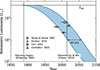 |
Fig. 1. Evolution of the bolometric luminosity of V883 Ori during the outburst dimming phase. The symbols denote measurements from different studies, with horizontal bars showing the time range of adopted data. The blue band represents the adopted luminosity curve, which carries an uncertainty of ∼40 yr due to the uncertainties in estimating Lbol. |
2.3. Temperature model
We adopted a two-stream radiation transfer (2sRT) method to calculate the temperature (e.g., Hubeny 1990). The heating sources at each grid cell are due to irradiation (qirr), viscous dissipation (qvis), and latent heat exchange (qlatent). We computed qirr from the bolometric luminosity (equation (4)), while the viscous heating rate follows from the α-disk viscosity ( ) and the latent heating rate is proportional to the condensation rate (equation (3), see Wang et al. 2025). In the outburst active phase, the disk adjusts to a temperature and density structure determined by the bolometric luminosity, Lpk, assuming hydrostatic balance. In the dimming phase, following Flock et al. (2017), we let the disk adapt to a new equilibrium temperature obtained by the 2sRT (Teq) over a thermal relaxation timescale, dT/dt = (Teq − T)/trelax (see Appendix C for the calculation of trelax). The Rosseland mean opacity per unit gas mass, κR – a key quantity that determines trelax – is a free model parameter. In our simulation (see Sect. 3), due to the low metallicity and disk viscosity, the disk temperature is determined by irradiation, with qvis and qlatent contributing little.
2.4. Fitting ALMA observations
The intensity shoulder in V883 Ori is identified in both ALMA band 6 (0.038″, project code: 2015.1.00350.S, PI: Lucas Cieza) and band 7 (0.028″, project code: 2016.1.00728.S, PI: Lucas Cieza) high-resolution continuum images. We converted the continuum images into radial profiles by azimuthally averaging the data within concentric annuli of radial width 1/5 of the respective beam size. To fit the continuum profiles, we generated synthetic intensity profiles in both bands by conducting 2sRT with profiles for the dust temperature and density taken from the simulation results. The 2sRT was performed in a plane-parallel manner in the disk’s vertical direction, with the optical depth corrected for disk inclination i = 38.3° (Cieza et al. 2016). Pebble opacities for different sizes and ice fractions were computed with optool (Dominik et al. 2021), adopting the DSHARP optical constants (Birnstiel et al. 2018). After being convolved with the beam size, the synthetic intensity profiles were compared with the continuum data at 45–85 au, where the intensity shoulder lies.
Tobin et al. (2023) measured the column density of water isotope H O in band 5 (0.126″). Given the limited data sensitivity, we fit only the mean column density between 80–120 au in our simulations to the observed value, assuming an isotopic ratio 18O/16O = 1/560 (Wilson & Rood 1994). In reality, the observed water vapor abundance may be influenced by processes beyond simple recondensation (Sect. 3.2). Therefore, we introduced an additional free parameter, fcond, such that −dρvap/dt = fcondℛcond.
To incorporate observational constraints from both continuum and water emission, we applied a log-normal likelihood for each dataset. Each likelihood was then weighted and combined by the number of beams covered by the area of interest (see equations (E.1) and (E.2)).
3. Results
We conducted Markov chain Monte Carlo (MCMC) analysis with emcee (Foreman-Mackey et al. 2013) to obtain the posterior distribution (see Appendix E). The parameter’s posterior values are given in Table 1.
Overview of MCMC parameters and posterior values ([16,50,84]-th percentiles) for both the retreating snowline and static snowline model.
3.1. Emergence of intensity shoulder
The best-fit results are shown in Fig. 3, where the synthetic intensity profiles agree well with the dual-band data, especially capturing the intensity shoulder feature at 50–70 au (gray-shaded region). To understand this, we plot the time evolution of the corresponding surface density profiles in Fig. 2. As the disk cools during the outburst dimming phase, vapor gradually recondenses on pebbles, creating a bump in surface density at the condensation front, which appears in continuum as the intensity shoulder. Matching the observed position of the shoulder requires the snowline to retreat to ≈60 au at the observational epoch (t′ = 121 yr). This places a stringent constraint on the thermal relaxation time, or IR opacity, κR, of the disk. If the disk had cooled more rapidly (lower κR), the snowline would already have retreated inside 50 au, shifting the shoulder much closer to the star, within the expected observational time.
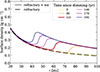 |
Fig. 2. Time evolution of the surface density profiles of the best-fit model. Silicate surface density remains constant with time. The thick line denotes the best fit, t′ = 121 yr. |
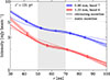 |
Fig. 3. Comparison of the synthetic intensity profiles with ALMA continuum. Crosses show ALMA data adopted from Houge et al. (2024), spaced according to the beam sizes; shaded regions indicate the rms error. Solid lines represent the best-fit retreating snowline model, while dotted lines correspond to the best-fit static model. Enhanced emission toward the inner regions arises likely from intense viscous heating (Alarcón et al. 2024), which is not accounted for in the model. |
Simultaneously fitting the dual-band continuum yields St0 ≈ 0.01, corresponding to a maximum grain size of around a centimeter. The need to have centimeter-sized particles in the disk follows from the low spectral indices at 50–70 au (α = 2.5 − 3.0), a result consistently found across ALMA band 3-7 in V883 Ori by Houge et al. (2024).
3.2. Extended water emission
The mean column density of H O at 80–120 au, as estimated from our models assuming optically thin emission, is presented in Fig. 4. In all simulated cases, the water abundance drops sharply within the first 110 years, and transitions to a slowly evolving stage afterward. This is due to different condensation timescales in the disk’s midplane and the upper layers (see Appendix D). After the snowline retreats, vapor in the midplane recondenses rapidly. Conversely, in the disk’s upper layer, where pebble densities are much lower, the recondensation time can reach ∼102 − 103 yr (Visser et al. 2015; Rab et al. 2017). Therefore, due to the lag caused by the finite recondensation time, the snowline inferred from molecular emission would consistently appear further away than its actual position during the outburst dimming phase. Our modeling shows that an enhanced condensation rate (fcond ≈ 4) is required to match the inferred water vapor abundance, which may indicate a shallower size distribution and/or porous grains (Birnstiel 2024), both of which increase the total dust surface area at the disk atmosphere. In addition, the destruction of water by photodissociation, heterogeneous nucleation, and different outburst durations may also influence the observed gas-phase water abundance (Fischer et al. 2023; Ros & Johansen 2024; Romero-Mirza et al. 2024).
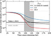 |
Fig. 4. Average column density of H |

3.3. The need for a retreating snowline model
A retreating snowline naturally explains the distant intensity shoulder and the extended water emission, relics of the earlier outburst. In contrast, a static snowline model fails to explain the observations (Fig. 3 and Fig. E.2). To illustrate this, we performed another MCMC simulation, where the disk structure is set by a constant Lbol (treated as a free parameter) rather than evolving with the luminosity curve. In other words, the temperature and vapor equilibrium instantly adapt to the stellar luminosity. Because of the instantaneous adjustment, the static model fails to maintain a sufficient amount of vapor in the outer disk: the best-fit water number density is ≈7σ away from the observed value (Fig. 4). Furthermore, in the static model, the snowline is located at ≈30 au, failing to reproduce the shoulder feature at 50–70 au in the observed intensity profile.
4. Conclusions and discussions
We investigated V883 Ori’s continuum and water line emission with a retreating snowline model. The key findings are:
-
The dimming stage of a stellar outburst results in a receding water snowline. Vapor condensation at the snowline front creates a bump in surface density, marking the transition from icy to ice-free pebbles.
-
Vapor in the disk upper layer takes ∼102 − 103 yr to recondense, leading to substantial amounts of water vapor in the outer disk, even after the snowline has retreated inward. The observed H218O outside the current snowline region (50–70 au) is a leftover of a much hotter past phase.
-
The retreating snowline model simultaneously reproduces the intensity shoulder feature in ALMA band 6/7 continuum and the extended water emission. In contrast, a static model fails to maintain the snowline at 50–70 au under the present-day luminosity.
In our modeling, both the disk cooling time (trelax), which controls the snowline retreat speed, and the millimeter opacity, which sets the continuum emission, depends on dust opacities. Thus, the thermal history of outburst systems constrains dust properties. For example, the retreating snowline model requires κR ≈ 4.6 cm2 g−1, whereas a self-consistent calculation from the DSHARP opacity yields κR ≈ 0.4 cm2 g−1. This mismatch implies excess IR opacity relative to millimeter opacities, possibly arising from a non-MRN size distribution, carbon-rich small grains (Woitke et al. 2016), or porous dust (Zhang et al. 2023). Under the assumed dimming curve of luminosity, our model predicts that the intensity shoulder will move by 10 au over 25 years (Fig. 2), a trend testable with future observations. With ALMA’s growing sample of outburst systems at high resolution, we expect the intensity shoulder to emerge as a ubiquitous feature of large-scale water phase transitions in disks.
Acknowledgments
The authors thank for useful discussion with Vardan Elbakyan, Shangjia Zhang, Hanpu Liu. This work is supported by the National Natural Science Foundation of China under grant Nos. 12233004 and 12473065.
References
- Alarcón, F., Casassus, S., Lyra, W., Pérez, S., & Cieza, L. 2024, MNRAS, 527, 9655 [Google Scholar]
- Allen, D. A., Strom, K. M., Grasdalen, G. L., Strom, S. E., & Merrill, K. M. 1975, MNRAS, 173, 47P [Google Scholar]
- Aumatell, G., & Wurm, G. 2011, MNRAS, 418, L1 [NASA ADS] [CrossRef] [Google Scholar]
- Birnstiel, T. 2024, ARA&A, 62, 157 [NASA ADS] [CrossRef] [Google Scholar]
- Birnstiel, T., Ormel, C. W., & Dullemond, C. P. 2011, A&A, 525, A11 [NASA ADS] [CrossRef] [EDP Sciences] [Google Scholar]
- Birnstiel, T., Dullemond, C. P., Zhu, Z., et al. 2018, ApJ, 869, L45 [CrossRef] [Google Scholar]
- Carvalho, A. S., Hillenbrand, L. A., & Kóspál, Á. 2025, ApJ, 993, 38 [Google Scholar]
- Cieza, L. A., Casassus, S., Tobin, J., et al. 2016, Nature, 535, 258 [Google Scholar]
- Cieza, L. A., Ruíz-Rodríguez, D., Perez, S., et al. 2018, MNRAS, 474, 4347 [CrossRef] [Google Scholar]
- Connelley, M. S., & Reipurth, B. 2018, ApJ, 861, 145 [NASA ADS] [CrossRef] [Google Scholar]
- Contreras Peña, C., Johnstone, D., Baek, G., et al. 2020, MNRAS, 495, 3614 [Google Scholar]
- Dominik, C., Min, M., & Tazaki, R. 2021, OpTool: Command-line driven tool for creating complex dust opacities, Astrophysics Source Code Library [record ascl:2104.010] [Google Scholar]
- Dubrulle, B., Morfill, G., & Sterzik, M. 1995, Icarus, 114, 237 [Google Scholar]
- Fischer, W. J., Hillenbrand, L. A., Herczeg, G. J., et al. 2023, in Protostars and Planets VII, eds. S. Inutsuka, Y. Aikawa, T. Muto, K. Tomida, & M. Tamura, ASP Conf. Ser., 534, 355 [NASA ADS] [Google Scholar]
- Flock, M., Nelson, R. P., Turner, N. J., et al. 2017, ApJ, 850, 131 [Google Scholar]
- Foreman-Mackey, D., Hogg, D. W., Lang, D., & Goodman, J. 2013, PASP, 125, 306 [Google Scholar]
- Furlan, E., Fischer, W. J., Ali, B., et al. 2016, ApJS, 224, 5 [Google Scholar]
- Houge, A., & Krijt, S. 2023, MNRAS, 521, 5826 [NASA ADS] [CrossRef] [Google Scholar]
- Houge, A., Macías, E., & Krijt, S. 2024, MNRAS, 527, 9668 [Google Scholar]
- Hubeny, I. 1990, ApJ, 351, 632 [NASA ADS] [CrossRef] [Google Scholar]
- Kóspál, Á., Ábrahám, P., Akimkin, V. V., et al. 2025, A&A, 703, A20 [NASA ADS] [CrossRef] [EDP Sciences] [Google Scholar]
- Laznevoi, S. I., Akimkin, V. V., Pavlyuchenkov, Y. N., et al. 2025, A&A, 700, L24 [NASA ADS] [CrossRef] [EDP Sciences] [Google Scholar]
- Leemker, M., van’t Hoff, M. L. R., Trapman, L., et al. 2021, A&A, 646, A3 [EDP Sciences] [Google Scholar]
- Liu, H., Herczeg, G. J., Johnstone, D., et al. 2022, ApJ, 936, 152 [NASA ADS] [CrossRef] [Google Scholar]
- Mathis, J. S., Rumpl, W., & Nordsieck, K. H. 1977, ApJ, 217, 425 [Google Scholar]
- Nakajima, T., Nagata, T., Nishida, M., Sato, S., & Kawara, K. 1986, MNRAS, 221, 483 [Google Scholar]
- Öberg, K. I., Facchini, S., & Anderson, D. E. 2023, ARA&A, 61, 287 [CrossRef] [Google Scholar]
- Pickering, E. C. 1890, Ann. Harv. College Obs., 18, 113 [Google Scholar]
- Rab, C., Elbakyan, V., Vorobyov, E., et al. 2017, A&A, 604, A15 [NASA ADS] [CrossRef] [EDP Sciences] [Google Scholar]
- Romero-Mirza, C. E., Banzatti, A., Öberg, K. I., et al. 2024, ApJ, 975, 78 [NASA ADS] [CrossRef] [Google Scholar]
- Ros, K., & Johansen, A. 2013, A&A, 552, A137 [NASA ADS] [CrossRef] [EDP Sciences] [Google Scholar]
- Ros, K., & Johansen, A. 2024, A&A, 686, A237 [NASA ADS] [CrossRef] [EDP Sciences] [Google Scholar]
- Saito, E., & Sirono, S.-I. 2011, ApJ, 728, 20 [NASA ADS] [CrossRef] [Google Scholar]
- Schoonenberg, D., & Ormel, C. W. 2017, A&A, 602, A21 [NASA ADS] [CrossRef] [EDP Sciences] [Google Scholar]
- Shakura, N. I., & Sunyaev, R. A. 1973, A&A, 24, 337 [NASA ADS] [Google Scholar]
- Smith, S. A., Romero-Mirza, C. E., Banzatti, A., et al. 2025, ApJ, 984, L51 [Google Scholar]
- Strom, K. M., & Strom, S. E. 1993, ApJ, 412, L63 [Google Scholar]
- Tobin, J. J., van’t Hoff, M. L. R., Leemker, M., et al. 2023, Nature, 615, 227 [NASA ADS] [CrossRef] [Google Scholar]
- van ’t Hoff, M. L. R., Tobin, J. J., Trapman, L., et al. 2018, ApJ, 864, L23 [Google Scholar]
- Viscardi, E. M., Macías, E., Zagaria, F., et al. 2025, A&A, 695, A147 [NASA ADS] [CrossRef] [EDP Sciences] [Google Scholar]
- Visser, R., Bergin, E. A., & Jørgensen, J. K. 2015, A&A, 577, A102 [NASA ADS] [CrossRef] [EDP Sciences] [Google Scholar]
- Wang, Y., Ormel, C. W., Mori, S., & Bai, X.-N. 2025, A&A, 696, A38 [NASA ADS] [CrossRef] [EDP Sciences] [Google Scholar]
- Wilson, T. L., & Rood, R. 1994, ARA&A, 32, 191 [Google Scholar]
- Woitke, P., Min, M., Pinte, C., et al. 2016, A&A, 586, A103 [NASA ADS] [CrossRef] [EDP Sciences] [Google Scholar]
- Zhang, S., Zhu, Z., Ueda, T., et al. 2023, ApJ, 953, 96 [NASA ADS] [CrossRef] [Google Scholar]
Appendix A: Bolometric luminosity measurements
The onset of the outburst in V883 Ori was not directly observed. But it likely starts before A.D. 1888, when the reflection nebula IC 430 was observed to be illuminated by the outburst (Pickering 1890), as argued by Strom & Strom (1993). By fitting the spectral energy distribution, the bolometric luminosity of V883 Ori was estimated to be 400 L⊙ (Strom & Strom 1993) in the 1980s (Allen et al. 1975; Nakajima et al. 1986) and had significantly decreased to 218 L⊙ (Furlan et al. 2016; Connelley & Reipurth 2018) in about 20 years. Given the typical month-to-year rise time of FUors (e.g., Fischer et al. 2023), it is very likely that V883 Ori has been in the dimming phase since A.D. 1888.
However, estimating the bolometric luminosity of V883 Ori is fraught with substantial uncertainty. As a young stellar object, it suffers severe extinction and reddening at near-infrared wavelengths from dusty proto-stellar envelopes. In the mid-infrared, where extinction is less severe, observations are hindered by heavy saturation in modern surveys like WISE (Contreras Peña et al. 2020). Liu et al. (2022) derived a much higher bolometric luminosity of ≈647 L⊙ by accounting for the reddening. Unlike most works adopting discrete photometric data, recently, Carvalho et al. (2025) fits the medium resolution spectrophotometry within a range of 0.4–2.5 μm and found excellent match to even broader spectrum across 0.4–4.2 μm. They yielded an accretion luminosity of 458 L⊙, which lies well inside the assumed luminosity curve (Fig. 1).
Appendix B: Dust model
At each radius, we modeled the pebble size distribution by constructing several size bins spanning radii from smax and smin. For small pebbles (e.g., sp < 0.1 cm), logarithmic spacing was used, whereas for larger ones, the size bins are more evenly spaced. The pebble surface density for each size bin (Σp, i) was then obtained by dividing Σp into these size bins according to the MRN distribution  . For each size bin i, its Stokes number (Sti) is obtained by scaling the pebble size at the bin center (sp, i) with smax, assuming that the pebbles follow the Epstein drag law: i.e., Sti, 0 = St0sp, i/smax. Then the 2D pebble density distribution is obtained by adopting normal distribution in the vertical direction:
![Mathematical equation: $$ \begin{aligned} \rho _{{\mathrm{p} },i} (z) = \rho _{{\mathrm{p} },0} \exp \left[ -\frac{1}{2} \left( \frac{z}{H_{{\mathrm{p} },i}}\right)^2 \right]. \end{aligned} $$](/articles/aa/full_html/2025/11/aa57233-25/aa57233-25-eq25.gif) (B.1)
(B.1)
Here Hp, i is the scale height of pebbles in the size bin i, following Dubrulle et al. (1995):
![Mathematical equation: $$ \begin{aligned} H_{{\mathrm{p} },i} (z)= H_{\mathrm{g} } \left[ 1 + \frac{\mathrm{St} _{i,0}}{\alpha }\left(\frac{2 H_{\mathrm{g} }^{2}}{z^{2}}\right)\left(\exp \left(\frac{z^{2}}{2 H_{\mathrm{g} }^{2}}\right)-1\right) \right]^{-1/2}. \end{aligned} $$](/articles/aa/full_html/2025/11/aa57233-25/aa57233-25-eq26.gif) (B.2)
(B.2)
In equation (B.2), the vertical variation in the Stokes number due to gas stratification was accounted for,  . The gas scale height, Hg, was determined in the outburst active phase, after iterating between the gas density distribution, assuming hydrostatic balance, and the temperature structure calculated from 2sRT. Given Σp, i, the midplane pebble density, ρp, 0, can be obtained by integrating the vertical density distribution following equation (B.1).
Recently, Houge et al. (2024) preformed dust evolution modeling and demonstrated that, to match the observed spectral index in V883 Ori, pebble sizes should not evolve appreciably during the swift outburst event. Therefore, we maintain a constant pebble size distribution throughout the outburst dimming phase.
Given the size distribution, the total surface area of pebbles per unit volume can be obtained by summing over all size bins,
 (B.3)
(B.3)
which is used to compute the vapor recondensation rate ℛcond. The number density of particles in each size bin is given as np, i = ρp, i/mp, i, where  is the particle mass. We adopt
  as the internal density of pebbles, assuming a compact ice-silicate mixture with half ice in mass (e.g., Schoonenberg & Ormel 2017).
Appendix C: Thermal relaxation timescale
Following Flock et al. (2017), we combine the optically thin and optically thick limits to determine the thermal relaxation time:
 (C.1)
(C.1)
where lmfp = 1/(κRρg) is the mean free path of photons,  is the radiation diffusion coefficient and Hphot is the height of disk photosphere (τR = 2/3), as measured from the simulation. Here Cv = 8.2 × 10⁷ erg g−1 K−1 is the specific heat capacity of the He-H2 mixture (assuming 71% H2 and ideal gas) and κR is the Rosseland mean opacity per gas mass, which is a free parameter.
Appendix D: 2D structure of retreating snowline
To illustrate the evolution of disk’s thermal structure during the outburst dimming phase, we present 2D snapshots of our best-fit simulation results at different times since Lbol declines in Fig. D.1. We focus on three epochs: t′ = 110 yr (the observational epoch) and two additional snapshots taken 50 yr before (when recondensation just begins) and after (when most vapor has recondensed in the outer disk) this point (see Fig. 4). At each time, the disk temperature, vapor condensation timescale (tcond) and number density of water vapor (nH2O) are shown. The condensation timescale is defined as tcond = ρvap/ℛcond.
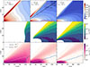 |
Fig. D.1. Disk temperature, vapor condensation timescale (tcond), and number density of water (nH2O) during the outburst dimming phase of the best-fit model. Here t′=t − tbeg is the time lapse since the bolometric luminosity started to decline. The value of Lbol corresponding to this time is labeled. In the top row, the range of 140-150 K is shaded in white to highlight the snowline region. At t′ = 121 yr – the present epoch – the emission surfaces (τmm = 2/3) of ALMA band 5, 6 and 7 and disk photosphere (see Sect. C) are plotted along with the temperature contour. In the middle row, the region where no condensation occurs is plotted in white. In the bottom row, two lines denoting ice(vapor)-to-gas ratio of 10−3 are indicated to highlight the snowline region. |
As Lbol decreases, the temperature drops in the entire disk, with the midplane cooling slower due to the large infrared optical depth. This difference in cooling time renders the midplane hotter than the upper layer, which is also found in Laznevoi et al. (2025). Concurrently, vapor recondenses and the snowline retreats, as shown in the bottom row of Fig. D.1. The middle row of Fig. D.1 shows the condensation timescale. In the upper layer of the disk, tcond is significantly longer than near the midplane, leaving uncondensed vapor plumes in the disk atmosphere (bottom row). This explains the slowly declining tail in the time evolution of the water column density (Fig. 4). This “inertia” in vapor’s response to changing luminosity was recently observed in DQ Tau, where the cold water abundance shows little reaction to variations in accretion luminosity on timescales of days to weeks (Kóspál et al. 2025). Radially, tcond reaches a minimum value at ∼80 − 100 au, increasing outward due to lower pebble densities and inward due to higher temperature. Notably, this increase in condensation timescale was also reported by Smith et al. (2025) in their modeling of EX Lup, implied by the higher water abundance toward the outer disk (their Fig. 10). The ice freezing-out timescale in EX Lup, constrained by multi-epoch observations of Spitzer and JWST (Smith et al. 2025), is one magnitude shorter (∼10 yr) than calculated from our simulations. This difference is expected, given the much larger pebble number density in EX Lup’s inner disk.
Finally, we plot the emission surfaces in our 2sRT calculation (upper row, middle panel), where the millimeter optical depth (τmm) equals 2/3. There is a clear elevation of the emission surface across snowline at ≈60 au, rising from the recondensation of vapor. As the emission surfaces trace different disk layers thus different temperature, we expect that the continuum emission will not only depend on the surface density distribution but also be modulated by the disk temperature structure. For molecular emission of water at band 5, because τmm ≈ 0.7 at the midplane of 80 au, we only expect minor dust attenuation on measuring the mean water column density at 80-120 au.
Appendix E: MCMC analysis
To fit the ALMA observations, we adopt a log-normal likelihood for each dataset:
 (E.1)
(E.1)
where  is either the azimuthally averaged continuum intensity of the n-th annulus in band i (I) or the mean water column density between 80-120 au (
 ). Correspondingly,
  is the synthetic data from the simulations. Following Viscardi et al. (2025),
  refers to the fractional root mean square (rms) error of the mean within annulus n, where Bi is the beam area of band i and An is the area corresponding to annulus n. For the
  emission, the area spanning 80 to 120 au is treated as a single annulus. Then the joint log-likelihood reads:
 (E.2)
(E.2)
With this joint likelihood, MCMC analysis was performed for both the retreating snowline model and the static snowline model. In the static model, the parameters t′ and fcond are replaced by a single Lbol, which controls the temperature structure together with the opacity κR in the IR band (Sect. 2.3). Gaussian priors are used for t′ (σt′ = 10 yr) and Lbol (σLbol = 110 L⊙), assuming that the uncertainties in the luminosity curve span 2σ range (i.e., the luminosity curve spans 40 yr). Other parameters adopt uniform priors. For Zpeb, St0, fcond and κR, sampling is carried out in logarithmic space.
We ran MCMC until all parameters converged over > 50 correlation timescales. The resulting posterior distributions are shown in Figs. E.1 and E.2, with values summarized in Table 1. In the retreating snowline model, several correlations can be seen among disk parameters (Zpeb, γ, γpeb and St0) and the gas density slope γ remains poorly constrained. These degeneracies are expected since the adopted disk model parameters do not directly correspond to the observational diagnostics. Specifically, the following features are noted:
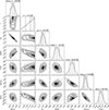 |
Fig. E.1. Corner plot of retreating snowline model. The dashed lines indicate 16th, 50th, and 84th percentiles of the posterior distribution. |
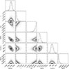 |
Fig. E.2. Corner plot of static snowline model. |
-
The parameter St0, which determines the maximum grain size, is positively correlated with Zpeb and negatively correlated with γ and γpeb. First, the Stokes number of pebbles decreases in denser gas. A shallower (larger) γ, which implies a higher gas density at 60 au, thus requires a smaller St0 to maintain the same smax of ∼ cm, as suggested by the spectral indices (see Sect. 3.1). Second, pebble size affects the continuum emission differently across the disk. In the inner disk where smax ≫ mm, increasing the pebble size significantly reduces the millimeter opacity. In the outer disk where smax ≈ mm, however, opacity becomes less sensitive to smax (e.g., Birnstiel et al. 2018). Consequently, increasing St0 both reduces the overall continuum intensity and flattens its radial slope, necessitating larger Zpeb and a steeper surface density profile (lower γpeb) to fit the data.
-
The gas density slope γ is negatively correlated with Rosseland mean opacity κR. This arises since to reproduce the intensity shoulder, the snowline should retreat to ≈60 au at the expected observation time (t′), following the assumed luminosity curve. Because the gas density and κR together govern the disk’s cooling time (trelax), that is, the retreat speed, γ and κR are naturally related. Furthermore, the posterior of κR essentially follows the assumed Gaussian prior of t′.
-
Large γ (toward the upper bound) is preferred. This can be understood as follows: during the outburst dimming phase, the outer disk cools faster than the inner regions, steepening the temperature gradient over time (Laznevoi et al. 2025). A higher γ (shallower density profile) therefore tends to equalize the cooling rate across the disk, "tilting" the intensity profile toward a plateau, as being observed. A value γ > −1 may fit the data even better, but such flat profiles are implausible.
-
The factor fcond, which controls the condensation rate, is negatively correlated with κR. An increase in κR slows the retreat of the snowline (larger t′), allowing a reduced fcond to achieve similar condensation levels.
From Fig. 3, we find that the model underestimates the emission within 40 au and correspondingly, struggles to capture the declining spectral index toward inner disk. These discrepancies likely arise from intense viscous heating (Alarcón et al. 2024) and optically thick environment (Tobin et al. 2023) in V883 Ori’s inner disk., which is included in the model. Simple power-law profiles, as adopted in this work, cannot simultaneously reproduce both the inner and outer disk, implying a sharp transition in the disk properties of V883 Ori.
In the static snowline model, many parameters are driven toward the edges of their prior ranges, indicating that the model cannot adequately reproduce the data. In particular, the disk struggles to reach sufficiently high temperatures. Consequently, κR and γ are pushed to their minimum value, and Lbol is constrained to the upper wing of its Gaussian prior, trying to obtain maximum penetration of stellar photons into the disk midplane regions.
All Tables
Overview of MCMC parameters and posterior values ([16,50,84]-th percentiles) for both the retreating snowline and static snowline model.
All Figures
|
Fig. 1. Evolution of the bolometric luminosity of V883 Ori during the outburst dimming phase. The symbols denote measurements from different studies, with horizontal bars showing the time range of adopted data. The blue band represents the adopted luminosity curve, which carries an uncertainty of ∼40 yr due to the uncertainties in estimating Lbol. |
| In the text | |
|
Fig. 2. Time evolution of the surface density profiles of the best-fit model. Silicate surface density remains constant with time. The thick line denotes the best fit, t′ = 121 yr. |
| In the text | |
|
Fig. 3. Comparison of the synthetic intensity profiles with ALMA continuum. Crosses show ALMA data adopted from Houge et al. (2024), spaced according to the beam sizes; shaded regions indicate the rms error. Solid lines represent the best-fit retreating snowline model, while dotted lines correspond to the best-fit static model. Enhanced emission toward the inner regions arises likely from intense viscous heating (Alarcón et al. 2024), which is not accounted for in the model. |
| In the text | |
|
Fig. 4. Average column density of H |
| In the text | |
|
Fig. D.1. Disk temperature, vapor condensation timescale (tcond), and number density of water (nH2O) during the outburst dimming phase of the best-fit model. Here t′=t − tbeg is the time lapse since the bolometric luminosity started to decline. The value of Lbol corresponding to this time is labeled. In the top row, the range of 140-150 K is shaded in white to highlight the snowline region. At t′ = 121 yr – the present epoch – the emission surfaces (τmm = 2/3) of ALMA band 5, 6 and 7 and disk photosphere (see Sect. C) are plotted along with the temperature contour. In the middle row, the region where no condensation occurs is plotted in white. In the bottom row, two lines denoting ice(vapor)-to-gas ratio of 10−3 are indicated to highlight the snowline region. |
| In the text | |
|
Fig. E.1. Corner plot of retreating snowline model. The dashed lines indicate 16th, 50th, and 84th percentiles of the posterior distribution. |
| In the text | |
|
Fig. E.2. Corner plot of static snowline model. |
| In the text | |
Current usage metrics show cumulative count of Article Views (full-text article views including HTML views, PDF and ePub downloads, according to the available data) and Abstracts Views on Vision4Press platform.
Data correspond to usage on the plateform after 2015. The current usage metrics is available 48-96 hours after online publication and is updated daily on week days.
Initial download of the metrics may take a while.