| Issue |
A&A
Volume 704, December 2025
|
|
|---|---|---|
| Article Number | A37 | |
| Number of page(s) | 13 | |
| Section | Numerical methods and codes | |
| DOI | https://doi.org/10.1051/0004-6361/202451015 | |
| Published online | 28 November 2025 | |
An adaptive parameter estimator for poor-quality spectral data of white dwarfs
1
School of Mathematics and Statistics, Shandong University, Weihai,
264209
Shandong,
PR
China
2
School of Business, Shandong University, Weihai,
264209
Shandong,
PR
China
3
School of Airspace Science and Engineering, Shandong University, Weihai,
264209
Shandong,
PR
China
★★ Corresponding author: This email address is being protected from spambots. You need JavaScript enabled to view it.
Received:
7
June
2024
Accepted:
16
September
2025
Abstract
White dwarfs represent the end stage for 97% of stars, making precise parameter measurement crucial for understanding stellar evolution. Traditional estimation methods involve fitting spectra or photometry, which require high-quality data. In recent years, machine learning has played a crucial role in processing spectral data due to its speed, automation, and accuracy. However, two common issues have been identified. First, most studies rely on data with high signal-to-noise ratios (S/N > 10), leaving many poor-quality datasets underutilized. Second, existing machine learning models, primarily based on convolutional and recurrent networks and their variants, fail to simultaneously capture both local spatial and long-range sequential spectral information. To address these challenges, we designed the estimator network (EstNet), an advanced algorithm integrating multiple techniques, including residual networks, squeeze and excitation attention, gated recurrent units, adaptive loss, and Monte Carlo dropout. A total of 5965 poor-quality white dwarf spectra (R~1800, S/N~1.17) were used for the experiments. EstNet achieved average percentage errors of 13.81% for effective temperature and 3.92% for surface gravity on the test set. These results are superior to other mainstream algorithms and consistent with the outcomes of traditional theoretical spectrum fitting methods. In the future, our algorithm will be applied to large-scale parameter estimations on data from the China Space Station Survey Telescope and the Dark Energy Spectroscopic Instrument.
Key words: line: profiles / methods: data analysis / methods: statistical / catalogs / stars: fundamental parameters / white dwarfs
These authors contributed equally to this work.
© The Authors 2025
 Open Access article, published by EDP Sciences, under the terms of the Creative Commons Attribution License (https://creativecommons.org/licenses/by/4.0), which permits unrestricted use, distribution, and reproduction in any medium, provided the original work is properly cited.
This article is published in open access under the Subscribe to Open model. This email address is being protected from spambots. You need JavaScript enabled to view it. to support open access publication.
1 Introduction
Accurately measuring the atmospheric physical parameters of white dwarfs is crucial for studying stellar evolution and the structure of the Milky Way, given the significant role white dwarfs play in various astronomical phenomena. For instance, Type Ia supernovae, which result from the explosion of white dwarfs in close binary systems, are key to understanding cosmic distances (Bildsten et al. 2007; Qi et al. 2022). Double white dwarfs are the primary sources of gravitational waves detected by the Laser Interferometer Space Antenna (Finch et al. 2023). In addition, the luminosity function of white dwarfs is used to estimate the ages of star clusters (Bedin et al. 2019; Cukanovaite et al. 2023) and their mass function can measure the stellar death rate and also estimate the age of the galactic halo (Liebert et al. 2005; Kalirai 2013). Investigating the proper motions of white dwarfs is useful in studies of the distribution of dark matter in the galactic halo (Torres et al. 2002). Overall, white dwarfs are vital for investigating stellar evolution and the structure of the Milky Way.
White dwarfs are compact stars characterized by a low luminosity, high density, high surface temperature, blue-white color, and radiation concentrated in the ultraviolet band. Approximately 97% of stars in the Milky Way will eventually evolve into white dwarfs (Parsons et al. 2020; Almeida et al. 2023). The initial masses of stars that become white dwarfs at the end of their lives range from 8.5 to 10.6 M⊙ and they experience mass loss during evolution. Currently, observed white dwarfs have masses primarily ranging from 0.5 to 0.8 M⊙ (Woosley & Heger 2015). Additionally, Wang et al. (2022a) discovered 21 white dwarfs with masses not exceeding 0.3 M⊙ in the Gaia DR2 and LAMOST DR8. The effective temperatures of white dwarfs range from 4000 to 150 000 K, and the average surface gravity acceleration is 108 cm s−2 (log g = 8). Their apparent magnitudes are concentrated at 15.5m. The faintest known white dwarf has a luminosity of 10−4.7 L⊙ (Fontaine et al. 2001), and most have luminosities between 10−2 and 10−3 L⊙ (McCook & Sion 1999). Their radii typically range from 0.008 to 0.023 R⊙ (Fontaine et al. 2001). This study focuses on estimating surface gravity, log g, and effective temperature, Teff.
In stellar parametrization, two main approaches are commonly employed: forward approaches and discriminative methods. Forward approaches, such as Cannon (Ness et al. 2015), utilize data-driven methods to model spectra from well-calibrated reference objects. By relying on the physical consistency of reference labels, such as those derived from cluster isochrones or high-resolution spectroscopy, rather than explicit covariance modeling, these approaches maintain statistical consistency. Conversely, discriminative methods such as Payne (Ting et al. 2019) employ neural networks to directly map spectra to parameters, offering significant computational advantages in speed and scalability. However, this efficiency comes with a trade-off, as such methods can introduce systematic distortions in posterior covariances. For error sensitive analyses requiring robust uncertainty quantification, forward modeling is the preferred approach, as it ensures a more accurate treatment of covariances. In contrast, discriminative methods excel in scenarios where rapid parameter estimation is prioritized, particularly in data-rich environments where speed and scalability are crucial. With the increasing availability of large-scale survey data, discriminative methods, such as deep learning, have been frequently applied in astronomy.
Traditional methods generally have higher estimation accuracy for stellar atmospheric physical parameters but are less efficient when dealing with large amounts of poor-quality data. For photometric data, traditional methods use color indices to calculate atmospheric physical parameters for different spectral types of stars (Crawford 1958; Alonso et al. 1999; Kirby et al. 2008). Color indices are calculated based on photometric magnitudes in various bands, which can be influenced by interstellar reddening and extinction, thereby affecting the calculation. For spectral data, atmospheric physical parameters are mostly estimated through template matching (Barbuy et al. 2003; Lee et al. 2011) or line index methods (Thomas et al. 2002; Ting et al. 2019). Template matching relies on the distance between theoretical and observed spectra and requires high-quality observed spectra. Low-resolution and low-S/N spectra contain a lot of noise. The line index method relies on flux information at specific wavelengths and does not consider the entire spectrum, limiting its effectiveness when spectral data are incomplete.
Recently, there have been advancements in estimating the parameters of white dwarfs. Chen & Liu (2024) leveraged Bayesian methods to estimate the parameters of white dwarfs. Liang et al. (2024) estimated the stochastic gravitational-wave background (SGWB) of white dwarfs using weak-signal limits. Suleimanov et al. (2024) employed hydrostatic local thermodynamic equilibrium atmosphere models to estimate the mass of white dwarfs. Castro-Tapia et al. (2024) developed a mixing length theory (MLT) incorporating thermal diffusion and composition gradients to analyze crystallization-driven convection in carbon-oxygen white dwarfs. Ferreira et al. (2024) estimated the physical and dynamical parameters of white dwarfs through interpolations with theoretical models and evolutionary tracks. Panthi et al. (2024) used TESS data to construct light curves and combined light curves with multi-wavelength spectral energy distributions (SEDs) to estimate the luminosity, temperature, and radius of white dwarfs. Theoretical models are established under certain assumptions, such as isolated stars or stars in binary systems with uniformly distributed ambient media, no mass loss, and no complex material exchange. However, these assumptions may not fully match actual observations, and recent works have focused on further optimizing white dwarf atmospheric models (Chen 2022; Ferrand et al. 2022; Camisassa et al. 2022).
With the continuous release of large-scale survey data, the volume of astronomical data is expected to grow exponentially. The vast amount of spectral data requires rapid, efficient, and timely processing. Traditional astronomical methods, which rely on expert knowledge and manual supervision to estimate atmospheric physical parameters, will face significant challenges. However, the rapid development of deep learning technology offers new opportunities for estimating these parameters. Smith & Geach (2023) argued that the symbiotic relationship between large, high-quality, multi-modal public datasets in astronomy and cutting-edge deep learning research can lead to mutual benefits. Neural networks, a crucial component of deep learning, simulate the neural circuits of human brain and mathematically characterize the Hebbian rule (Sejnowski & Tesauro 1989). With the introduction of backpropagation algorithms (LeCun et al. 1988), solutions to the vanishing and exploding gradient problems (Hochreiter 1998; Rehmer & Kroll 2020), and improvements in computer hardware resources, neural networks have become indispensable in the artificial intelligence era (Kumar & Thakur 2012; Wu & Feng 2018), impacting astronomical research as well.
In recent years, many researchers have used deep learning techniques to estimate stellar parameters, such as fully connected neural networks (FCNs; Pan & Li 2017; Li & Wang 2025), convolutional neural networks (CNNs; Leung & Bovy 2019; Wu et al. 2020, 2024), and recurrent neural networks (RNNs; Li & Lin 2023; Luo et al. 2024). However, each of these deep learning networks has its limitations. FCNs have a large number of parameters, requiring high computational and storage resources, making them unsuitable for feature extraction as the backbone network. CNNs focus on the local spatial information of input data in each layer and perform poorly when processing data with sequential dependencies (Zuo et al. 2015). RNNs can handle and capture the time step sequence information of input data, but they may encounter gradient vanishing and exploding problems when capturing long-term dependencies (Hochreiter & Schmidhuber 1997).
The spectra of white dwarfs contain many characteristic absorption lines, such as DA-type white dwarfs exhibiting prominent Balmer absorption lines (McCook & Sion 1987). Each type of spectral line is distributed at different wavelengths and is interrelated. In manual spectral classification, researchers analyze these lines to classify the spectral types of white dwarfs or estimate their parameters by fitting the Balmer absorption lines (Zhao et al. 2013). For a white dwarf spectrum, it is essential to locate the local spatial information of specific absorption lines, while taking into account the dependencies among them, commonly known as sequence information. Therefore, there is an urgent need for an algorithm that can extract both spatial and sequence information from spectra.
High-quality data enables researchers to provide more accurate parameter estimates, but such data are often scarce within the vast amounts of survey data. Therefore, extracting valuable information from poor-quality data is crucial. Raw observed data must undergo a series of processes, including extraction, calibration, and sky subtraction, to generate one-dimensional spectra. Failing to utilize poor-quality data results in significant data waste. Currently, most parameter estimation tasks rely on high-signal-to-noise ratio (S/N>10) spectral data (Tremblay et al. 2011; Kong et al. 2018a; Li et al. 2022; Guo et al. 2022; Xiang et al. 2022). The absorption lines of white dwarfs are mainly concentrated in the blue end (3900–5900 Å) (Kong et al. 2018b). In our study, the spectral data has a resolution of 1800, with a median S/N of 3.135 and a mode of 1.17 in the u-band, characterizing it as poor-quality spectral data, as shown in Fig. 1. Low-resolution and low-S/N data exhibit poorer quality, with missing flux and significant noise, as shown in Fig. 2. To address this issue, we propose an adaptive loss mechanism that enables the model to focus more on learning from non-anomalous data and less from anomalous data, thereby improving the robustness of parameter estimation. The main goal of this work has been to develop the estimator network (EstNet) for estimating the atmospheric physical parameters of white dwarfs: surface gravity, log g, and effective temperature, Teff. The four main contributions are as follows.
We propose an adaptive loss mechanism that drives EstNet to learn from non-anomalous data, reducing its reliance on anomalous data and decreasing the model’s sensitivity to anomalies.
EstNet integrates the design principles of a CNN and an RNN, enabling it to capture both local spatial information and global sequence information from spectral data. This approach overcomes the limitations of existing methods and enhances the model’s ability to learn from poor-quality data.
The output of EstNet is no longer a single point estimate, but an interval estimate of the labels, allowing for the measurement of model uncertainty and improving interpretability.
Our reliability analysis, comparative analysis, robustness analysis, saliency analysis, and validation analysis on EstNet demonstrate EstNet’s effectiveness from multiple perspectives.
The structure of this paper is as follows. Section 2 introduces the EstNet model framework. Section 3 describes the datasets. Section 4 explains the training process of EstNet and evaluates its estimation performance from multiple perspectives. In Sect. 5, we compare and validate our work against the traditional parameter estimation methods used by Guo et al. (2015) and Kepler et al. (2021). Finally, the detailed conclusions and future outlook are presented in Sect. 6.
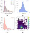 |
Fig. 1 Data description. (a) Signal-to-noise ratio distribution across the u, g, r, i, z bands from LAMOST. White dwarfs’ characteristics are primarily concentrated in the u band, with a median S/N of 3.14 and a mode of 1.17, indicating extremely poor data quality. (b) Distribution of log g labels, primarily concentrated around 8 dex. (c) Distribution of Teff labels, primarily concentrated around 20 000 K. (d) Two-dimensional histogram of the distribution in the parameter space. |
2 Methods
2.1 EstNet overview
Our primary goal is to design an algorithm that can capture both the local spatial information of specific spectral lines and the long-range dependencies between different absorption lines. In astronomy, deep learning algorithms are mainly applied in the form of CNNs or RNNs (Bambharolia 2017; Sherstinsky 2020). However, these algorithms cannot simultaneously extract both spatial and sequential information from spectra. The spectral sequence length is usually longer than the convolution kernel size. CNNs have difficulties with extracting local features and their global interconnection at the same time. Different absorption lines have dependencies and the key information in the spectra may be global and span multiple bands. To capture long-range dependencies, sequence models represented by RNNs can be used. However, RNNs may struggle to learn long-term dependencies (He et al. 2016a), caused by vanishing or exploding gradients during the backpropagation stage (Rojas & Rojas 1996) in the training process. The Residual Network (ResNet), proposed by Kaiming He and colleagues from Microsoft Research Asia, has had a significant impact in the field of CNNs (He et al. 2016a). The residual connections in ResNet effectively address the network degradation problem, allowing the model to deepen and improve accuracy, while ensuring convergence (He et al. 2016b). This has garnered substantial attention from both academia and industry. ResNet has profoundly influenced subsequent network designs, and residual connections are now widely used in modern neural networks. In EstNet, each PRSE (PReLU and Squeeze-and-Excitation) block in the PRSE module consists of two residual connections.
The memory capacity of neurons in an RNN is limited. With the data being continuously fed into the model, previously accumulated information tends to be forgotten. An effective solution is to introduce gating mechanisms to control the accumulation of information in the hidden state. These gates selectively add new information and forget previously accumulated information, retaining only what is valuable for prediction. Networks with such gating mechanisms include the long short-term memory (LSTM) and gated recurrent unit (GRU) (Shiri et al. 2024). In LSTM, the input gate, forget gate, and output gate work in unison to regulate the input, retention, and output of information, ensuring effective updating of the cell state. However, compared to the GRU, LSTM has a more complex structure with more parameters. In a GRU network, only the update gate and reset gate are used to balance the input of new information and the forgetting of irrelevant information. These aspects simplify the model structure and reduce computational complexity and memory requirements. This design improves training efficiency and often achieves better performance than LSTM in many applications. EstNet incorporates GRU cells to capture the global sequence information of spectra, thereby retaining memory that is beneficial for the final predictions.
Originally, CNNs were primarily employed to extract local spatial information from an image. Taking the operation of a two-dimensional convolutional kernel as an example, we define [X]i+a,j+b as the pixel value at (i + a, j + b) of input image, [H]i,j as the pixel value at (i, j) of feature map, [V]a, b as the kernel parameter at (a, b), and u as the bias term. [H]i,j is a weighted sum of [X]i+a,j+b, within the range |a| < Δ, |b| < Δ. This process, as shown in Eq. (1), reflects the locality of the convolutional kernel, depending solely on the correlations between adjacent pixels, expressed as
![Mathematical equation: $\[[\boldsymbol{H}]_{i, j}=u+\sum_{a=-\Delta}^{\Delta} \sum_{b=-\Delta}^{\Delta}[\boldsymbol{V}]_{a, b} \times[\boldsymbol{X}]_{i+a, j+b}.\]$](/articles/aa/full_html/2025/12/aa51015-24/aa51015-24-eq1.png) (1)
(1)
When performing convolution operations on a one-dimensional spectrum, the entire process can be formulated for the output feature point [H]i as Eq. (2), where [V]k denotes the kernel parameter, u signifies a bias term and [X]i+k represents the original feature point, expressed as
![Mathematical equation: $\[[\boldsymbol{H}]_i=u+\sum_{k=-\Delta}^{\Delta}[\boldsymbol{V}]_k \times[\boldsymbol{X}]_{i+k}.\]$](/articles/aa/full_html/2025/12/aa51015-24/aa51015-24-eq2.png) (2)
(2)
GRU is primarily used to extract global sequential information. In our model, after numerous convolution operations, the feature sequence is denoted as xB,512,L/16, where B represents the batch size, 512 is the number of channels, and L/16 is the sequence length. As shown in Eq. (7), after passing through the GRU, the output is a feature sequence with only a single channel, denoted as xB,1,L/16. This process effectively integrates the information from 512 different channels, capturing global information, and generates a representative feature sequence with one channel. The computation process of GRU follows
![Mathematical equation: $\[\widetilde{H_t}=\tanh \left(X_t W_{x h}+\left(R_t \odot H_{t-1}\right) W_{h h}+b_h\right),\]$](/articles/aa/full_html/2025/12/aa51015-24/aa51015-24-eq3.png) (3)
(3)
![Mathematical equation: $\[H_t=Z_t \odot H_{t-1}+\left(1-Z_t\right) \odot \widetilde{H}_t,\]$](/articles/aa/full_html/2025/12/aa51015-24/aa51015-24-eq4.png) (4)
(4)
where Xt ∈ RB×L/16 denotes the t-th channel input feature, Ht ∈ RB×L/16 denotes the t-th channel hidden state, Ht−1 ∈ RB×L/16 is the previous hidden state, Zt ∈ RB×L/16 represents the update gate, Rt ∈ RB×L/16 denotes the reset gate, and ⊙ is hadamard product. Wxh ∈ RL/16×L/16, Whh ∈ RL/16×L/16, and bh ∈ R1×L/16 are parameters. Here, tanh(·) is the nonlinear activation function. The gating mechanism in GRU selectively retains information from the hidden state and the input sequence, reducing the memory burden on the network.
In designing the algorithm, we incorporated principles from the aforementioned algorithms and introduced attention mechanisms to enhance the focus on important spectral features. Inspired by the human nervous system, attention mechanisms selectively filter information and focus on what is important at a given moment (Niu et al. 2021). Currently, there are various types of attention mechanisms, including multi-head attention, channel attention, and spatial attention, which have shown excellent results in fields such as speech recognition, text generation, machine translation, and image classification (He et al. 2016a). For the spectral data, we need neural networks to focus more on important spectral features (e.g., hydrogen Balmer absorption lines) to enhance the learning capabilities. Therefore, we introduced the squeeze and excitation (SE) attention mechanism following the residual connection in EstNet (Hu et al. 2018).
EstNet integrates mainstream neural network design principles, combining various techniques into one neural network model. The backbone network incorporates a CNN and an RNN (Bambharolia 2017; Sherstinsky 2020). A fully connected feedforward neural network outputs the predicted labels (Sazlı 2006). We proposed an adaptive loss mechanism and embedded Monte Carlo dropout to measure model uncertainty, providing confidence intervals for the estimates and enhancing model interpretability (Kendall & Gal 2017). To deepen the model, we introduced residual connections in the PRSE blocks of EstNet, allowing the model to handle more complex estimation tasks (He et al. 2016a). To prevent internal covariate shift, we included batch normalization layers after each convolutional layer (Ioffe & Szegedy 2015; Bjorck et al. 2018). Our training strategy employed weight decay and learning rate decay to improve model convergence (D’Angelo et al. 2024). To enhance the model’s representation learning capability, we incorporated the SE attention mechanism in the PRSE module (Hu et al. 2018). Next, we introduce the main components of EstNet.
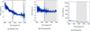 |
Fig. 2 Set of poor-quality spectra. The blue line shows the trend of original flux as a function of wavelength. The gray shaded area indicates anomalous flux in the spectrum. The original spectra are LAMOST DR7 low-resolution spectra, which have undergone relative flux calibration. |
2.2 EstNet structure
EstNet consists of four modules: the input module, the PRSE module, the GRU module, and the output module, as shown in Fig. 3.
Input module: the input data x is a three-dimensional tensor with a shape of (B, C, L), representing batch size, channel number, and length, respectively; x passes through a convolutional layer with a kernel size of 3, which increases the input channels to 64 without changing the size of x. Then it goes through a batch normalization (BN) layer and is activated by the PReLU function, resulting in the final output xB,64,L. The process is described in Eq. (5) and the function is expressed as
![Mathematical equation: $\[x_{B, 64, L}=\operatorname{Input}\left(x_{B, 1, L}\right)=\operatorname{PReLU}\left(\operatorname{BN}\left(\operatorname{Conv}_3\left(x_{B, 1, L}\right)\right)\right).\]$](/articles/aa/full_html/2025/12/aa51015-24/aa51015-24-eq5.png) (5)
(5)
PRSE module: the PRSE module is composed of multiple stacked PRSE blocks. Residual connections, originally proposed in ResNet, address network degradation issues (He et al. 2016a). The PRSE block incorporates two chained residual connections. The first residual connection outputs multi-channel feature maps, while the second applies different weights to each channel, enabling the network to focus on important channel information (Hu et al. 2018). The process is expressed as
![Mathematical equation: $\[x_{B, 512, L / 16}=\operatorname{PRSE}\left(\operatorname{PRSE}\left(\ldots \operatorname{PRSE}\left(x_{B, 64, L}\right) \ldots\right)\right).\]$](/articles/aa/full_html/2025/12/aa51015-24/aa51015-24-eq6.png) (6)
(6)
GRU module: the GRU network is a type of RNNs that introduces multiple gating mechanisms to effectively solve long-term dependency issues (Bengio et al. 1993; Dey & Salem 2017). It models the dependencies of absorption lines at different wavelengths, extracting global sequence information from the entire spectrum. The input to the GRU cell at each time step is down-sampled by a factor of 16. By integrating information from different channels to capture global information, it ultimately produces a single-channel feature map xB,1,L/16, expressed as
![Mathematical equation: $\[x_{B, 1, L / 16}=\operatorname{GRU}\left(x_{B, 512, L / 16}\right).\]$](/articles/aa/full_html/2025/12/aa51015-24/aa51015-24-eq7.png) (7)
(7)
Output module: the output module flattens the three-dimensional tensor xB,1,L/16 into a two-dimensional tensor xB,L/16, and then passes it through a fully connected layer to obtain the final output. A dropout layer is introduced before the fully connected layer, utilizing Monte Carlo dropout to deactivate hidden neurons with a certain probability, thereby enhancing the model’s generalization ability (Kendall & Gal 2017). This process is expressed as
![Mathematical equation: $\[x_{B, 1}=\operatorname{Output}\left(x_{B, 1, L / 16}\right)=\operatorname{FC}\left(\operatorname{Flatten}\left(x_{B, 1, L / 16}\right)\right)=\operatorname{FC}\left(x_{B, L / 16}\right).\]$](/articles/aa/full_html/2025/12/aa51015-24/aa51015-24-eq8.png) (8)
(8)
 |
Fig. 3 EstNet architecture. EstNet comprises four parts: input module, PRSE module, GRU module, and output module, as shown in panels 1–4. Panel 5 illustrates two types of information presented in spectra: the local spatial information of a specific spectral line and the global dependencies between different absorption lines. Panel 6 describes the structure of the PRSE block, which determines the depth of EstNet. Panel 7 details the internal structure of the GRU cell, a neural component with memory capabilities. |
2.3 Adaptive loss
We designed an adaptive loss mechanism to specifically address poor spectral data. EstNet, being a highly parameterized deep neural network model, possesses strong learning capabilities. Our adaptive loss mechanism enables EstNet to dynamically adjust its focus during the learning process. Anomalies are typically rare in practice, comprising only a small fraction of the dataset. However, their presence can introduce learning bias in the early stages of training, as neural networks may overfit these irregular patterns due to their high loss or gradient magnitude. As a result, such samples often receive elevated anomaly scores. To address this, EstNet adaptively focuses on samples from dense data regions with lower anomaly scores, while downweighting those from sparse regions with high anomaly scores. This strategy enhances the overall robustness and performance. This approach to anomaly detection, based on neural networks (Han & Cho 2006), is widely used in other fields as well. For example, LSTM and VAE have achieved significant success in anomaly detection in time series data (Ergen & Kozat 2019; Niu et al. 2020; Zhou et al. 2021).
In the first stage, EstNet measures the anomaly degree of each sample. In the second stage, EstNet loads the anomaly information obtained from the first stage, then performs limited learning on the anomalous samples and extensive learning on the non-anomalous samples. ![Mathematical equation: $\[D=\left\{(x^{(n)}, y^{(n)})\right\}_{n=1}^{N}\]$](/articles/aa/full_html/2025/12/aa51015-24/aa51015-24-eq9.png) is a dataset of a size, N. Then,
is a dataset of a size, N. Then, ![Mathematical equation: $\[D_{\text {train}}=\left\{(x^{(n)}, y^{(n)})\right\}_{n=1}^{O}\]$](/articles/aa/full_html/2025/12/aa51015-24/aa51015-24-eq10.png) is the training set, where O is the training set size. fθ(x) = f(x, θ) refers to the EstNet network used in our study, which can be considered as a nonlinear function. fθ(x) ∈ ℱ, where ℱ is a set of functions. θ ∈ Ω, θ is a learnable parameter, and Ω is the parameter space.
is the training set, where O is the training set size. fθ(x) = f(x, θ) refers to the EstNet network used in our study, which can be considered as a nonlinear function. fθ(x) ∈ ℱ, where ℱ is a set of functions. θ ∈ Ω, θ is a learnable parameter, and Ω is the parameter space.
In the first phase, we consider the Huber loss function, Lstep1(y, fθ(x)), defined as Eq. (9), where δ is a small constant. When the residual is less than or equal to δ, Lstep1 reduces to the L2 loss. Otherwise, Lstep1 reduces to the L1 loss, ensuring the model’s differentiability at the origin (Meyer 2021; Wang et al. 2022b). Lstep1 is expressed as
![Mathematical equation: $\[L^{\text {step1 }}\left(y, f_\theta(x)\right)= \begin{cases}\frac{1}{2}\left(y-f_\theta(x)\right)^2, & \left|y-f_\theta(x)\right| \leq \delta, \\ \delta\left|y-f_\theta(x)\right|-\frac{1}{2} \delta^2, & \left|y-f_\theta(x)\right|>\delta.\end{cases}\]$](/articles/aa/full_html/2025/12/aa51015-24/aa51015-24-eq11.png) (9)
(9)
The parameters in fθ(x) are initialized using a normal distribution. The learning algorithm employs mini-batch gradient descent (Bottou 2010), which randomly selects a small subset of training samples during each iteration to compute the gradients and update the parameters. In the t-th iteration, the algorithm randomly selects a subset γt containing K samples and computes the average gradient of the loss function for each sample in this subset. The parameters are updated using Eq. (10), with α as the learning rate,
![Mathematical equation: $\[\theta_{t+1} \leftarrow \theta_t-\alpha \frac{1}{K} \sum_{(x, y) \in \gamma_t} \frac{\partial L^{\mathrm{step} ~1}(y, f(x; \theta))}{\partial \theta}.\]$](/articles/aa/full_html/2025/12/aa51015-24/aa51015-24-eq12.png) (10)
(10)
Given the threshold ε, the model stops learning when Eq. (11) is satisfied and the learned parameters θstep1 are saved,
![Mathematical equation: $\[\left|L\left(y, f_\theta(x)\right)\right|<\varepsilon, \forall x \in D_{\text {train }}.\]$](/articles/aa/full_html/2025/12/aa51015-24/aa51015-24-eq13.png) (11)
(11)
By loading the parameters θstep1 from the first stage, we obtained the model fθstep1 (x). Using Eq. (12), we can calculate the absolute distance α(y | x) between the predicted and true values for each sample in Dtrain. Equation (13) normalizes the absolute distance to obtain the bias score β(y | x) for each sample, where αmin and αmax are the minimum and maximum values of all α(y | x) in Dtrain, respectively,
![Mathematical equation: $\[\alpha(y \mid x)=\left|y-f_{\theta^{\text {step 1 }}}(x)\right|,\]$](/articles/aa/full_html/2025/12/aa51015-24/aa51015-24-eq14.png) (12)
(12)
![Mathematical equation: $\[\beta(y \mid x)=\frac{\alpha(y \mid x)-\alpha_{\min }}{\alpha_{\max }-\alpha_{\min }}.\]$](/articles/aa/full_html/2025/12/aa51015-24/aa51015-24-eq15.png) (13)
(13)
In the second stage, we employ Eq. (14) to perform kernel density estimation on the labels ![Mathematical equation: $\[\{y^{(n)}\}_{n=1}^{O}\]$](/articles/aa/full_html/2025/12/aa51015-24/aa51015-24-eq16.png) to calculate the probability score g(y), where O is the size of the training set, and H is the bandwidth. Our model employs the Gaussian kernel function k(y), as shown in Eq. (15):
to calculate the probability score g(y), where O is the size of the training set, and H is the bandwidth. Our model employs the Gaussian kernel function k(y), as shown in Eq. (15):
![Mathematical equation: $\[g(y)=\frac{1}{O} \sum_{i=1}^O \frac{1}{H} k\left(\frac{y^i-y}{H}\right),\]$](/articles/aa/full_html/2025/12/aa51015-24/aa51015-24-eq17.png) (14)
(14)
![Mathematical equation: $\[k(y)=\frac{1}{\sqrt{2 \pi}} \exp \left(-\frac{1}{2} y^2\right).\]$](/articles/aa/full_html/2025/12/aa51015-24/aa51015-24-eq18.png) (15)
(15)
Then, we can calculate weights for each sample of Dtrain by Eq. (16), where ϕ1 and ϕ2 are differentiable functions, referred to as the control functions, g(y) and β(y | x) represent the probability score and bias score, respectively, and γ is a balancing constant,
![Mathematical equation: $\[s(y, x)=\gamma \times \phi_1(g(y))+(1-\gamma) \times \phi_2(\beta(y \mid x)).\]$](/articles/aa/full_html/2025/12/aa51015-24/aa51015-24-eq19.png) (16)
(16)
The control functions determine how the probability score and bias score influence the weight calculation. In this study, the control functions are set as monotonic functions, as show in Eq. (17). In the Teff task, γ is set to 0, while in the log g task, γ is set to 0.1. For samples whose physical parameters are densely distributed, such as in the log g task, the incorporation of the probability score provides a more effective means to quantify sample anomalies, which is sensitive to extreme values. Conversely, for samples with parameters exhibiting greater dispersion, as in the Teff task, the anomaly measurement relies solely on the prediction bias,
![Mathematical equation: $\[s(y, x)=\gamma g(y)+(1-\gamma)(1-\beta(y \mid x)).\]$](/articles/aa/full_html/2025/12/aa51015-24/aa51015-24-eq20.png) (17)
(17)
Using the parameters θstep1 from the first stage as the initial parameters for the second stage reduces the training time. The second stage loss function is adaptively adjusted based on s(y, x) obtained from the first stage, ensuring minimal learning on anomalous samples and extensive learning on non-anomalous samples. The loss function for the second stage Lstep2, is defined as Eq. (18):
![Mathematical equation: $\[L^{\text {step2 }}\left(y, f_\theta(x)\right)= \begin{cases}\frac{1}{2} s(y, x)\left(y-f_\theta(x)\right)^2, & \left|y-f_\theta(x)\right| \leq \delta, \\ \delta s(y, x)\left|y-f_\theta(x)\right|-\frac{1}{2} \delta^2, & \left|y-f_\theta(x)\right|>\delta.\end{cases}\]$](/articles/aa/full_html/2025/12/aa51015-24/aa51015-24-eq21.png) (18)
(18)
The mini-batch gradient descent is then used again as the learning algorithm to optimize Lstep2 with the initial parameter set to θstep1. When the model converges again, the optimal parameters θopt are obtained, resulting in the optimal model fθopt(x), as shown in Eq. (19):
![Mathematical equation: $\[f_{\theta^{\text {opt }}}(x)=\arg \min _{\theta \in \Omega} L^{\text {step2 }}\left(y, f_\theta(x)\right).\]$](/articles/aa/full_html/2025/12/aa51015-24/aa51015-24-eq22.png) (19)
(19)
2.4 Monte Carlo dropout layer
Monte Carlo dropout is commonly employed to estimate the uncertainty of model predictions in neural networks. This technique involves performing multiple forward passes during inference, with different neurons randomly dropped each time. The results of these multiple passes are then statistically analyzed to estimate the uncertainty in the output (Gal & Ghahramani 2016). This uncertainty encompasses both inherent data noise and parameter uncertainty in the model (Kendall & Gal 2017). EstNet integrates Monte Carlo dropout in its output module to evaluate prediction confidence, thereby enhancing the understanding of its predictive behavior across different regions.
Letting Z1 = {Zi,j}Q×Q ∈ ℝQ×Q and Z2 = {Zi,j}K×K ∈ ℝK×K be the random matrices, each element of Z1 and Z2 follows a Bernoulli distribution, Zi,j ~ Bernoulli(Pi,j). The final network output can be represented as ![Mathematical equation: $\[\hat{y}=\left(X\left(Z_{1} W_{1}\right)+m\right)\left(Z_{2} W_{2}\right)\]$](/articles/aa/full_html/2025/12/aa51015-24/aa51015-24-eq23.png) . Here, X ∈ R1×Q is the input feature vector, W1 ∈ RQ×K and W2 ∈ RK×K are learnable parameters, and m ∈ R1×K is the bias vector.
. Here, X ∈ R1×Q is the input feature vector, W1 ∈ RQ×K and W2 ∈ RK×K are learnable parameters, and m ∈ R1×K is the bias vector.
For T forward passes, the final estimate is given by Eq. (20), the uncertainty measurement ![Mathematical equation: $\[\operatorname{Var}\left(\hat{y}_{1}, \ldots, \hat{y}_{T}\right)\]$](/articles/aa/full_html/2025/12/aa51015-24/aa51015-24-eq24.png) is given by Eq. (21), and sometimes it can be further calculated using the standard deviation as uncertainty. Here,
is given by Eq. (21), and sometimes it can be further calculated using the standard deviation as uncertainty. Here, ![Mathematical equation: $\[W_{1}^{t}\]$](/articles/aa/full_html/2025/12/aa51015-24/aa51015-24-eq25.png) and
and ![Mathematical equation: $\[W_{2}^{t}\]$](/articles/aa/full_html/2025/12/aa51015-24/aa51015-24-eq26.png) are the parameter matrices for the t-th iteration, and
are the parameter matrices for the t-th iteration, and ![Mathematical equation: $\[\hat{y}_{t}\left(x \mid W_{1}^{t}, W_{2}^{t}\right)\]$](/articles/aa/full_html/2025/12/aa51015-24/aa51015-24-eq27.png) denotes the outcome of the t-th forward pass, with
denotes the outcome of the t-th forward pass, with ![Mathematical equation: $\[\hat{y}_{t} \in R^{1 \times K}\]$](/articles/aa/full_html/2025/12/aa51015-24/aa51015-24-eq28.png) , expressed as
, expressed as
![Mathematical equation: $\[\hat{y}=E(y \mid x) \approx T^{-1} \sum_{t=1}^T \hat{y}_t\left(x \mid W_1^t, W_2^t\right),\]$](/articles/aa/full_html/2025/12/aa51015-24/aa51015-24-eq29.png) (20)
(20)
![Mathematical equation: $\[\operatorname{Var}\left(\hat{y}_1, \ldots, \hat{y}_T\right) \approx(T-1)^{-1} \sum_{t=1}^T\left(\hat{y}_t-\hat{y}\right)^T\left(\hat{y}_t-\hat{y}\right).\]$](/articles/aa/full_html/2025/12/aa51015-24/aa51015-24-eq30.png) (21)
(21)
The Monte Carlo dropout layer measures the uncertainty of different estimates, returning a predictive range for each parameter. These procedures enhance the robustness and interpretability of the model.
2.5 Evaluation metrics
To comprehensively evaluate the performance of EstNet, we computed the mean absolute error (MAE), root mean square error (RMSE), mean absolute percentage error (MAPE), and median error (ME). Smaller values of these metrics indicate lower prediction errors and higher accuracy in the model’s predictions. The calculation methods for these four evaluation metrics are
![Mathematical equation: $\[\text { MAE }=M^{-1} \sum_{i=1}^M\left|f_{\theta_{\mathrm{opt}}}\left(x_i\right)-y_i\right|,\]$](/articles/aa/full_html/2025/12/aa51015-24/aa51015-24-eq31.png) (22)
(22)
![Mathematical equation: $\[\mathrm{RMSE}=\sqrt{M^{-1} \sum_{i=1}^M\left(f_{\theta_{\mathrm{opt}}}\left(x_i\right)-y_i\right)^2},\]$](/articles/aa/full_html/2025/12/aa51015-24/aa51015-24-eq32.png) (23)
(23)
![Mathematical equation: $\[\text { MAPE }=M^{-1} \sum_{i=1}^M\left|\frac{f_{\theta_{\mathrm{opt}}}\left(x_i\right)-y_i}{y_i}\right|,\]$](/articles/aa/full_html/2025/12/aa51015-24/aa51015-24-eq33.png) (24)
(24)
![Mathematical equation: $\[\mathrm{ME}=\operatorname{Median}\left(\left|f_{\theta_{\mathrm{opt}}}\left(x_i\right)-y_i\right|\right).\]$](/articles/aa/full_html/2025/12/aa51015-24/aa51015-24-eq34.png) (25)
(25)
Here, fθopt (x) is the optimal model obtained after training, ![Mathematical equation: $\[D_{\text {test}}= \left\{(x^{(n)}, y^{(n)})\right\}_{n=1}^{M}\]$](/articles/aa/full_html/2025/12/aa51015-24/aa51015-24-eq35.png) represents the test set of size M selected from D, xi denotes the features of the i-th sample, and yi represents the true label of the i-th sample.
represents the test set of size M selected from D, xi denotes the features of the i-th sample, and yi represents the true label of the i-th sample.
3 Data
The LAMOST telescope, located at the Xinglong observatory of the national astronomical observatories, Chinese Academy of Sciences, is renowned for its significant aperture and extensive field of view (Su et al. 1998). It incorporates a unique Schmidt reflective design and is equipped with 4000 optical fibers on its focal plane, enabling the simultaneous observation of 4000 targets over a wide area. This configuration greatly enhances spectral acquisition efficiency (Yao et al. 2012). The LAMOST survey, in its seventh data release1, has provided 10 431 197 low-resolution spectra, including 9 846 793 stellar spectra, 198 272 galaxy spectra, 66 612 quasar spectra, and 319 520 spectra of unknown types. The extensive spectral data provided by LAMOST has significantly advanced our understanding and exploration of the Milky Way and its millions of stars.
Gentile Fusillo et al. (2021) utilized Gaia EDR3 to identify 1.3 million white dwarf candidates based on their absolute magnitude, color, and mass. Kong & Luo (2021) cross-matched these Gaia EDR3 white dwarf candidates with LAMOST DR7 data within a radius of 3″, obtaining 12 046 corresponding LAMOST spectra. Subsequently, they employed a support vector machine algorithm to further identify 9496 white dwarf candidates. After manual spectral verification, they confirmed 6190 white dwarfs. Using a template-matching method, they estimated the atmospheric parameters (log g, Teff) of the white dwarfs, providing a catalog of white dwarfs with estimated parameters. The white dwarfs in this catalog are mainly of DA and DB types.
Using the catalog provided by Kong & Luo (2021), we obtained low-resolution (R~1800) spectra from LAMOST DR7. These spectra have not undergone extinction correction or radial velocity correction. In the Teff task, to emphasize the overall distribution pattern of the entire spectrum, we applied min-max normalization to each spectrum (Song et al. 2024). In the log g task, to highlight the profiles of characteristic spectral lines, we constructed a spline curve to fit the continuum spectrum and normalized each pixel of the observed spectrum by dividing it by the corresponding continuum flux (Luo et al. 2019). Due to variations in the wavelength coverage of each spectrum in LAMOST, we applied a linear interpolation to ensure a uniform wavelength range from 4000 to 8000 Å for consistent input to the model, containing 3909 feature points. We implemented linear interpolation using the interpld function from the SciPy library2. After removing spectra without parameters or without S/Ns, or those with at least five consecutive flux values of zero, we obtained 5965 spectra for the experiments. All of these spectra correspond to single white dwarfs, as our method is not designed to handle binary systems. These spectra were then randomly partitioned into training, validation, and testing sets in an 8:1:1 ratio, with 80% allocated for training, 10% allocated for validation, and the remaining 10% reserved for testing. Before inputting the data into the model, both the features and labels also undergo Gaussian normalization. At the inference time, given the output of the model, this normalization is then inverted to restore the labels to the original scale.
The characteristic absorption lines of white dwarfs are primarily concentrated in the blue end (Kong et al. 2018b). In our experiment, the data quality was extremely poor, as shown in Figs. 1 and 2. The low-resolution and low-S/N spectral data exhibits issues such as flux loss and excessive noise. Compared to most studies that use high-S/N data (S/N > 10) for the parameter estimation, our task of conducting parameter estimation based on poor-quality data is highly challenging.
4 EstNet training and evaluation
4.1 Estimation of Teff and log g
Depending on the number of stacked PRSE blocks, we can define EstNet models of different depths. For white dwarfs, the main indicator of log g is the width of the atmospheric absorption lines (Kepler et al. 2021), while Teff is related to the flux intensity at different wavelengths (Prokhorov et al. 2009). We conducted extensive experiments to explore the impact of varying model complexities, as well as the estimation strategies of joint versus single estimation methods. We found that EstNet has greater difficulty capturing the width information of absorption lines than the flux intensity information. Therefore, we used the EstNet66 model, which has more parameters, to estimate log g, while the EstNet34 model as used to estimate Teff.
For the Teff estimation, we employed EstNet34, consisting of 34 convolutional layers. During training, a 0.6 dropout rate was applied to the fully connected layers, with a weight decay of 0.0008. For the log g estimation, we used EstNet66, which includes 66 convolutional layers. During training, a 0.75 dropout rate was applied to the fully connected layers, with a weight decay of 0.0015. We trained each model until the loss on the validation set did not improve for seven consecutive epochs and evaluated the model performance on the test set afterwards.
In Fig. 4, we present a comparison of the predicted values to the true labels. The scatter points are concentrated around the identity line, indicating that the predicted values are close to the true values. Specifically, the MAE, RMSE, MAPE, and ME for log g are 0.31 dex, 0.44 dex, 3.92%, and 0.22 dex, respectively. For Teff, the MAE, RMSE, MAPE, and ME are 3087 K, 5479 K, 13.81%, and 1672 K, respectively. Kong & Luo (2021) also provided the template matching errors for each white dwarf’s log g and Teff. On the test set, the average template matching errors are 465 K for Teff and 0.08 dex for log g, which are better than our results. Machine learning methods that rely on labels from traditional approaches are inherently an indirect learning process. This inevitably leads to further propagation and amplification of measurement errors, a common issue in works that use machine learning to estimate parameters from observed spectra. As shown in Fig. 5, compared to the optimal point estimates of a standard neural network, EstNet obtains the predictive distribution of the parameters of each sample through 200 forward sampling passes from the model’s parameter space, thereby enabling the construction of interval estimates for the parameters.
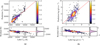 |
Fig. 4 Estimation results. (a) Estimation results for Teff. (b) Estimation results for log g. The upper subplots in both figures show the kernel density plots of predicted values and true labels, with yellow areas indicating high-density regions. The lower subplots show the residual distribution between predicted values and true labels. The horizontal axis represents true labels, and the vertical axis represents residuals and predicted values. The red solid line represents the identity line. |
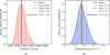 |
Fig. 5 Predictive distributions for a single sample. (a) Predictive distribution of Teff. (b) Predictive distribution of log g. The obsid refers to the observation ID of the target, sourced from LAMOST. The gray dashed lines measure the location at one standard deviation from the mean. |
4.2 Further discussion on spatial and sequential information
The formation of absorption and emission lines follows Kirchhoff’s law, reflecting distinct chemical compositions within the stellar atmosphere. CNNs primarily focus on the local spatial features of lines (Bambharolia 2017), while GRU is more adept at capturing the interdependencies between different lines (Shiri et al. 2024).
In the following, we sequentially output the feature spectra through the input module, PRSE module, and GRU module, as illustrated in Fig. 6. Due to the small number of convolution operations in the input module, the processed feature retains a high consistency with the input spectrum, with its resolution and sequence length (L) remaining unchanged, as shown in panels a and e of Fig. 6. The PRSE module involves numerous convolution and downsampling operations, resulting in a decrease in the resolution, reducing the sequence length from L to L/16, as shown in panels b and f of Fig. 6. Despite these operations, the spectral line information remains clearly visible, especially for the Hδ (~4100 Å), Hγ (~4300 Å), and Hβ (~4800 Å). Lines within the 4000–5000 Å range are not disrupted. This indicates that convolution operations primarily extract local spatial spectral line information, without disrupting the global structure of the entire spectrum.
As shown in panel c of Fig. 6, the global structure of the feature spectrum shows a noticeable change, with the overall feature spectrum curve exhibiting an upward trend. At the red end, the correlation between the fluctuations in the feature spectrum and the input spectrum is less apparent. As shown in panel g of Fig. 6, the Balmer lines of hydrogen are visible, but the fluctuations in other regions are difficult to interpret. The overall trend appears uneven. These are likely because the GRU module integrates information from different channels and captures the global dependencies between different spectral lines, significantly altering the global structure.
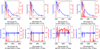 |
Fig. 6 Features from different network stages and saliency analysis. (a–c) Comparisons of the feature spectra (red line) extracted from the input module, PRSE module, and GRU module with the input spectra (blue line) when estimating Teff. (d) Model’s output response to the input spectra (blue line) when estimating Teff and the red line is saliency curve. (e–g) Comparisons of the feature spectra (red line) extracted from the input module, PRSE module, and GRU module with the input spectra (blue line) when estimating log g. (h) Model’s output response to the input spectra (blue line) when estimating log g and the red line is saliency curve. The normalized flux refers to either min-max (top panels) or continuum normalization (bottom panels). In both cases, a subsequent Gaussian normalization is also applied. The observation ID of this spectrum is 254115228. |
4.3 Reliability analysis
The Monte Carlo dropout layer in EstNet allows us to measure uncertainty in predictions for Teff and log g, thereby helping us analyze the reliability of the model’s outputs. The uncertainty is computed as the square root of Eq. (21), yielding the standard deviation. We conducted the uncertainty analysis on the test set. As shown in Fig. 7, the solid line represents the uncertainty trend, and the shaded area corresponds to the 95% confidence interval. When predictions approach the boundary of the training data, the prediction fluctuations of EstNet become more pronounced due to the smaller sample size, resulting in higher uncertainty and wider confidence intervals. When predictions approach the region where samples are concentrated, with log g close to 8 dex and Teff ranging from 10 000 to 30 000 K, the uncertainty becomes much lower, corresponding to significantly narrower confidence intervals. The uncertainty quantifies the consistency of the model’s multiple predictions for the same sample, enabling researchers to make reliable decisions.
4.4 Comparative analysis
With the advancement of machine learning, numerous algorithms have been applied to various astronomical tasks. However, there is still relatively little research available on the use of machine learning algorithms to estimate white dwarf parameters. We compared EstNet to other algorithms, including Random forest (Breiman 2001), XGBoost (Chen & Guestrin 2016), NGBoost (Duan et al. 2020), CatBoost (Prokhorenkova et al. 2018), and LightGBM (Ke et al. 2017). Additionally, we incorporated a multilayer perceptron (MLP) with our adaptive loss as a baseline (Kruse et al. 2022). It is structured as a fully connected feedforward network with four linear layers, each followed by a PReLU activation except for the output layer, enabling the model to capture complex representations.
Random forest algorithms have been widely used in the field of astronomy (Torres et al. 2019; Chandra et al. 2020; Echeverry et al. 2022; Guo et al. 2022). The new members of the Boosting family, Light-GBM and CatBoost, have also been widely adopted as commonly used machine learning algorithms. MLP is a fundamental neural network architecture in deep learning and is commonly used as a baseline in comparisons with more advanced deep learning models, where it has shown competitive performance in certain experimental evaluations. However, our EstNet exhibits a better predictive performance in all considered performance metrics than these models, as summarized in Tables 1 and 2.
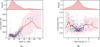 |
Fig. 7 Reliability analysis for Teff and log g. (a) Uncertainties on Teff. (b) Uncertainties on log g. The smooth curves represent the trend of uncertainty, and the shaded areas correspond to 95% confidence intervals. The density measures the distribution of the label values. |
Comparison with other models on Teff.
Comparison with other models on log g.
4.5 Robustness analysis
Our model is data-driven and our data are characterized by both low resolution and low S/N. The spectral data are very noisy, with issues such as missing flux and anomalous labels. However, with its inherent adaptive loss mechanism, EstNet can automatically reduce learning from anomalous data. To demonstrate EstNet’s robustness to noisy data, we went on to compare it to the LightGBM and CatBoost, which are widely used in astronomy (Coronado-Blázquez 2023; Xiao-Qing et al. 2024). We randomly selected 4772 spectra from 5965 spectra as the training set. Within the training set, we applied noise to the labels of 954 spectra, using a 2:8 ratio. For the Teff labels, the noise follows a normal distribution with a mean of 7000 K and a standard deviation of 100 K. For the log g labels, the noise follows a normal distribution with a mean of 1 dex and a standard deviation of 0.1 dex. For each task, we trained the model twice independently: once using the original training set and once using the same set with noise.
In Fig. 8, we display a dumbbell plot illustrating the fluctuations in various metrics before and after adding noise. Before adding noise, the errors of EstNet are smaller than those of LightGBM and CatBoost. For the Teff task, EstNet34 exhibits minimal fluctuation compared to LightGBM, as observed by the length of the lines in the plot. Therefore, EstNet34 not only has higher estimation accuracy than LightGBM, but also shows less performance degradation due to anomalous data, indicating better robustness. For log g task, EstNet66 has smaller errors than CatBoost before adding noise; after adding noise, the errors of both models are similar. The fluctuation in the evaluation metrics before and after adding noise is slightly larger for EstNet compared to CatBoost. This phenomenon is due to the varying degrees of dispersion in the log g and Teff labels. The log g labels are concentrated, with a standard deviation of 0.55 dex, while the Teff labels exhibit a large variation, with a standard deviation of 10 830 K. If the label values are more concentrated, particularly when there is noise in the labels, the learning process will become more challenging.
The outstanding performance of EstNet34 on Teff is remarkable. EstNet is designed to focus more on non-anomalous data in highly noisy and dispersed datasets. In contrast, boosting algorithms like LightGBM aim to reduce the fitting error of each base learner (Schapire 1999; Duffy & Helmbold 2002; Mayr et al. 2014) and anomalous samples often cause large fitting errors, leading the base learner to overly focus on these anomalies, which can sometimes be unnecessary. To further quantify the predictive behavior of EstNet, we conducted several experiments.
The output module generates the final predicted labels, and in order to explore the relationship between the model’s final output and the features of the input spectrum, we plotted saliency maps (Gomez & Mouchère 2023). For each spectrum, saliency was derived via backpropagation by calculating the gradient of the predicted labels with respect to the fluxes of the input spectrum, with the gradient magnitude serving as an indicator of the importance of each flux element (Springenberg et al. 2014). As shown in panels d and h of Fig. 6, the blue line represents the input spectrum after different normalizations, while the red line indicates the saliency values. When we estimate Teff, the saliency values at the blue end are notably higher and exhibit significant fluctuations, indicating that EstNet places greater emphasis on the features in the blue end (4000–5000 Å). During the log g task, the model primarily focuses on the feature line at 6500 Å, approximately corresponding to the Hα. Overall, the features that the model focuses on in the log g task are fewer than those it attends to in the Teff task. When the external factors include noise interference, the number of features that can be used to infer log g becomes further limited, rendering the prediction difficult.
To evaluate the capability in detecting anomalous samples, we performed control experiments on the Teff and log g estimation tasks. Figure 9 presents the outcomes of these experiments for Teff (top panels) and log g (bottom panels), where the left column shows the sample weight distribution without noise, while the right column indicates the scenario where we added artificial noise to the labels of 954 training samples (red points). It is evident that the weights associated with these red points in the right panels exhibit a greater dispersion and have a comparatively lower weight than before we added noise (see left panels). This confirms that the model autonomously detects anomalous samples and assigns them reduced weights accordingly. However, we also found that some blue points, which correspond to noise-free samples, also have reduced weights, indicating that the model may falsely detect some normal samples as anomalies. This phenomenon is particularly notable in the log g task, potentially leading to greater fluctuations in the evaluation metrics shown in Fig. 8.
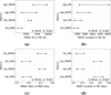 |
Fig. 8 Dumbbell plots of metric fluctuations before and after adding noise. (a) Fluctuations in RMSE and MAE for Teff between LightGBM and EstNet34. (b) Fluctuations in MAPE and ME for Teff between LightGBM and EstNet34. (c) Fluctuations in RMSE and MAE for log g between CatBoost and EstNet66. (d) Fluctuations in MAPE and ME for log g between CatBoost and EstNet66. The red points represent the metrics before adding noise, and the blue points represent the metrics after adding noise. The lengths of the lines indicate the degree of fluctuation in the evaluation metrics before and after adding noise. In b and d, the MAPE values have been scaled to match the magnitude of ME to facilitate convenient visualization. |
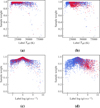 |
Fig. 9 Fluctuation of sample weights in the training set before and after adding noise. Top two panels show the results for Teff and the bottom two panels for log g. Indicated in red are the 954 training samples, where we added artificial noise to the labels in the right panels, while the blue training examples remained unchanged. |
5 Validation
Traditional methods for estimating white dwarf parameters primarily rely on theoretical models, which involve fitting the differences between observed and theoretical spectra. These techniques often require high-S/N and high-quality observed spectra. To demonstrate the validity of EstNet, we obtained spectral data from LAMOST, where the white dwarf parameters were estimated using traditional methods (Guo et al. 2015; Kepler et al. 2021), and we applied EstNet to this data.
Guo et al. (2015) combined three methods, colour-colour cut, LAMOST pipeline classification, and the width of Balmer lines, to select white dwarf candidates. These candidates were confirmed through visual inspection of spectra. To accurately estimate parameters, spectra with S/N > 10 were selected for absorption line fitting. For DA-type white dwarfs, Teff and log g were estimated by fitting the line profiles from Hβ to Hϵ. In practice, the line profiles of observed and theoretical spectra are normalized using two adjacent points on either side of each absorption line, ensuring that the line fitting is unaffected by flux calibration. The atmospheric models used in the fitting process were provided by Koester (2010). The widely used Levenberg-Marquardt nonlinear least-squares method, based on the steepest descent, was employed to fit the line profiles. The best model templates were fitted using the open-source IDL package MPFIT (Markwardt 2009).
Kepler et al. (2021) utilized SDSS DR16 data to classify and identify white dwarfs and subdwarfs. This dataset includes 2410 spectra, identifying 1404 DA-type, 189 DZ-type, 103 DC-type, and 12 DB-type. By simultaneously fitting the photometry and spectra for white dwarfs with S/N ≥ 10 and parallax error ≥ 4, they estimated Teff and log g. For white dwarfs with M-dwarf companions, the Hα line was excluded from the fitting process due to contamination.
Figure 10 shows the distribution of EstNet predictions compared to parameter estimates obtained using traditional methods. The red solid line represents the identity line. The scatter points of predicted values and true labels are mainly concentrated around the identity line, indicating that the predictions of EstNet is consistent with the parameters estimated using traditional methods. This validation strengthens confidence in EstNet and supports its application to large-scale automated parameter estimation in practice.
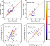 |
Fig. 10 Comparison with traditional methods in predicting log g and Teff of white dwarfs. The first row shows the predictions for Teff, while the second row displays the predictions for log g. The first column compares our results with those of Guo et al. (2015), using data from LAMOST. The second column compares our results with those of Kepler et al. (2021), using data from SDSS. The scatter point density in the yellow region is higher than in the purple region. The red solid line represents the identity line. The scatter points are distributed around the identity line, indicating that the predictions of EstNet are consistent and effective compared to traditional methods. |
6 Conclusion
When estimating the parameters of white dwarfs in practice, we find that the data are not only characterized by a low resolution, but extremely low S/N values as well. To address this issue, we designed the EstNet deep learning model, which has three notable advantages. First, we successfully combined a CNN, an RNN, and a FCN. EstNet captures both the local spatial information and the long-distance dependencies between different absorption lines. This gives it stronger learning capabilities, overcoming the limitations of existing astronomical research that relies solely on models based on CNNs or RNNs. Second, we designed an adaptive loss mechanism and embedded it into the EstNet model. This allows EstNet to automatically prioritize learning from non-anomalous data and minimize learning from anomalous data. Third, EstNet incorporates Monte Carlo dropout, enabling the measurement of uncertainty in the output labels. This enhances the interpretability of EstNet and allows users to reasonably assess the reliability of the estimated results.
To demonstrate the performance of EstNet, we conducted reliability analysis, comparative analysis, robustness analysis, and saliency analysis. For the log g and Teff estimation tasks, EstNet outperforms other widely used machine learning algorithms in astronomy across all considered evaluation metrics. In the Teff estimation task, the results of EstNet are less affected by noise compared to other models, highlighting its robustness in handling low-resolution, high-noise, and highly dispersed spectral data. Additionally, the results of EstNet are consistent with the white dwarf parameter estimates that were obtained using traditional methods on spectra with S/N ≥ 10, as performed by Guo et al. (2015) and Kepler et al. (2021), further validating the effectiveness of EstNet.
Ongoing surveys such as the Dark Energy Spectroscopic Instrument and 4-metre Multi-Object Spectrograph Telescope will continue to release more spectral data, a significant portion of which will be at low-resolution and low S/N. In the coming years, the China Space Station Survey Telescope will conduct deep sky surveys, obtaining vast amounts of seamless spectral data with a resolution of 200. A vast amount of low-quality spectral data urgently awaits effective utilization. In this study, we integrated the technique of anomaly detection and implemented the selective learning of samples based on deep learning methods. This learning approach relies on the guidance of an adaptive loss function, which needs to be carefully chosen based on the specific focus of different problems. In the future, expert prior knowledge, such as measurement errors on the physical parameters and S/Ns of the spectra, can also be incorporated into the loss function to achieve selective learning.
Data availability
Python scripts used in this study can be accessed at https://github.com/mystar365/ParaCode/tree/master.
Acknowledgements
We sincerely thank the anonymous referee for their professional comments, which have substantially helped us improve the manuscript. This study was supported by the Natural Science Foundation of Shandong Province with No.ZR2024MA063, No.ZR2022MA076 and No.ZR2022MA089, China Manned Space Project with No.CMS-CSST-2021-B05 and No.CMS-CSST-2021-A08, the National Natural Science Foundation of China (NSFC) with No. 11873037 and No.11803016, and the Young Scholars Program of Shandong University, Weihai, under grant 2016WHWLJH09. Thanks to the LAMOST team for releasing reliable spectra. Guoshoujing Telescope (the Large Sky Area MultiObject Fiber Spectroscopic Telescope LAMOST) is a National Major Scientific Project built by the Chinese Academy of Sciences. Funding for the project has been provided by the National Development and Reform Commission. LAMOST is operated and managed by the National Astronomical Observatories, Chinese Academy of Sciences. The LAMOST website is https://www.lamost.org/.
References
- Almeida, A., Anderson, S. F., Argudo-Fernández, M., et al. 2023, ApJS, 267, 44 [NASA ADS] [CrossRef] [Google Scholar]
- Alonso, A., Arribas, S., & Martínez-Roger, C. 1999, A&AS, 140, 261 [NASA ADS] [CrossRef] [EDP Sciences] [Google Scholar]
- Bambharolia, P. 2017, in ICAREM, 8 [Google Scholar]
- Barbuy, B., Perrin, M.-N., Katz, D., et al. 2003, A&A, 404, 661 [NASA ADS] [CrossRef] [EDP Sciences] [Google Scholar]
- Bedin, L., Salaris, M., Anderson, J., et al. 2019, MNRAS, 488, 3857 [NASA ADS] [CrossRef] [Google Scholar]
- Bengio, Y., Frasconi, P., & Simard, P. 1993, in ICNN, IEEE, 1183 [Google Scholar]
- Bildsten, L., Shen, K. J., Weinberg, N. N., & Nelemans, G. 2007, ApJ, 662, L95 [Google Scholar]
- Bjorck, N., Gomes, C. P., Selman, B., & Weinberger, K. Q. 2018, NeurIPS, 31 [Google Scholar]
- Bottou, L. 2010, in COMPSTAT (Berlin: Springer), 177 [Google Scholar]
- Breiman, L. 2001, Mach. Learn., 45, 5 [Google Scholar]
- Camisassa, M. E., Althaus, L. G., Koester, D., et al. 2022, MNRAS, 511, 5198 [NASA ADS] [CrossRef] [Google Scholar]
- Castro-Tapia, M., Cumming, A., & Fuentes, J. 2024, ApJ, 969, 10 [NASA ADS] [CrossRef] [Google Scholar]
- Chandra, V., Hwang, H.-C., Zakamska, N. L., & Budavári, T. 2020, MNRAS, 497, 2688 [NASA ADS] [CrossRef] [Google Scholar]
- Chen, Y. 2022, ApJ, 934, 34 [Google Scholar]
- Chen, T., & Guestrin, C. 2016, in KDD, 785 [Google Scholar]
- Chen, Z.-C., & Liu, L. 2024, Eur. Phys. J. C, 84, 1176 [Google Scholar]
- Coronado-Blázquez, J. 2023, MNRAS, 521, 4156 [Google Scholar]
- Crawford, D. L. 1958, ApJ, 128, 185 [Google Scholar]
- Cukanovaite, E., Tremblay, P.-E., Toonen, S., et al. 2023, MNRAS, 522, 1643 [NASA ADS] [CrossRef] [Google Scholar]
- D’Angelo, F., Andriushchenko, M., Varre, A. V., & Flammarion, N. 2024, NeurIPS, 37, 23191 [Google Scholar]
- Dey, R., & Salem, F. M. 2017, in MWSCAS, IEEE, 1597 [Google Scholar]
- Duan, T., Anand, A., Ding, D. Y., et al. 2020, in ICML, PMLR, 2690 [Google Scholar]
- Duffy, N., & Helmbold, D. 2002, Mach. Learn., 47, 153 [Google Scholar]
- Echeverry, D., Torres, S., Rebassa-Mansergas, A., & Ferrer-Burjachs, A. 2022, A&A, 667, A144 [NASA ADS] [CrossRef] [EDP Sciences] [Google Scholar]
- Ergen, T., & Kozat, S. S. 2019, IEEE Trans. Neural. Netw. Learn. Syst., 31, 3127 [Google Scholar]
- Ferrand, G., Tanikawa, A., Warren, D. C., et al. 2022, ApJ, 930, 92 [NASA ADS] [CrossRef] [Google Scholar]
- Ferreira, T., Saito, R. K., Minniti, D., et al. 2024, MNRAS, 527, 10737 [Google Scholar]
- Finch, E., Bartolucci, G., Chucherko, D., et al. 2023, MNRAS, 522, 5358 [NASA ADS] [CrossRef] [Google Scholar]
- Fontaine, G., Brassard, P., & Bergeron, P. 2001, PASP, 113, 409 [NASA ADS] [CrossRef] [Google Scholar]
- Gal, Y., & Ghahramani, Z. 2016, in ICML, PMLR, 1050 [Google Scholar]
- Gentile Fusillo, N., Tremblay, P.-E., Cukanovaite, E., et al. 2021, MNRAS, 508, 3877 [NASA ADS] [CrossRef] [Google Scholar]
- Gomez, T., & Mouchère, H. 2023, J. Electron. Imaging, 32, 020801 [Google Scholar]
- Guo, J., Zhao, J., Tziamtzis, A., et al. 2015, MNRAS, 454, 2787 [NASA ADS] [CrossRef] [Google Scholar]
- Guo, J., Zhao, J., Zhang, H., et al. 2022, MNRAS, 509, 2674 [NASA ADS] [Google Scholar]
- Han, S.-J., & Cho, S.-B. 2006, IEEE Trans. Syst. Man. Cybern. B Cybern., 36, 559 [Google Scholar]
- He, K., Zhang, X., Ren, S., & Sun, J. 2016a, in CVPR, 770 [Google Scholar]
- He, K., Zhang, X., Ren, S., & Sun, J. 2016b, in ECCV (Berlin: Springer), 630 [Google Scholar]
- Hochreiter, S. 1998, Int. J. Uncertainty Fuzz, 6, 107 [Google Scholar]
- Hochreiter, S., & Schmidhuber, J. 1997, Neural. Comput., 9, 1735 [Google Scholar]
- Hu, J., Shen, L., & Sun, G. 2018, in CVPR, 7132 [Google Scholar]
- Ioffe, S., & Szegedy, C. 2015, in ICML, pmlr, 448 [Google Scholar]
- Kalirai, J. S. 2013, Mem. Soc. Astron. Italiana, 84, 58 [Google Scholar]
- Ke, G., Meng, Q., Finley, T., et al. 2017, NeurIPS, 30 [Google Scholar]
- Kendall, A., & Gal, Y. 2017, NeurIPS, 30 [Google Scholar]
- Kepler, S. O., Koester, D., Pelisoli, I., Romero, A. D., & Ourique, G. 2021, MNRAS, 507, 4646 [NASA ADS] [CrossRef] [Google Scholar]
- Kirby, E. N., Guhathakurta, P., & Sneden, C. 2008, ApJ, 682, 1217 [Google Scholar]
- Koester, D. 2010, Mem. Soc. Astron. Ital., 81, 921 [Google Scholar]
- Kong, X., & Luo, A.-L. 2021, Res. Notes AAS, 5, 249 [CrossRef] [Google Scholar]
- Kong, X., Bharat Kumar, Y., Zhao, G., et al. 2018a, MNRAS, 474, 2129 [Google Scholar]
- Kong, X., Luo, A.-L., Li, X.-R., et al. 2018b, PASP, 130, 084203 [Google Scholar]
- Kruse, R., Mostaghim, S., Borgelt, C., Braune, C., & Steinbrecher, M. 2022, in Computational Intelligence - A Methodological Introduction (Berlin: Springer), 53 [Google Scholar]
- Kumar, K., & Thakur, G. S. M. 2012, Int. J. Inf. Technol. and Comput. Sci., 4, 57 [Google Scholar]
- LeCun, Y., Touresky, D., Hinton, G., & Sejnowski, T. 1988, Proc. Connectionist Models Summer Sch., 1, 21 [Google Scholar]
- Lee, Y. S., Beers, T. C., Prieto, C. A., et al. 2011, AJ, 141, 90 [NASA ADS] [CrossRef] [Google Scholar]
- Leung, H. W., & Bovy, J. 2019, MNRAS, 489, 2079 [CrossRef] [Google Scholar]
- Li, K., & Wang, L.-H. 2025, ApJS, 277, 51 [Google Scholar]
- Li, X., & Lin, B. 2023, MNRAS, 521, 6354 [NASA ADS] [CrossRef] [Google Scholar]
- Li, X., Wang, Z., Zeng, S., et al. 2022, RAA, 22, 065018 [Google Scholar]
- Liang, Z.-C., Li, Z.-Y., Li, E.-K., Zhang, J.-d., & Hu, Y.-M. 2024, Results Phys., 63, 107876 [Google Scholar]
- Liebert, J., Bergeron, P., & Holberg, J. 2005, ApJS, 156, 47 [NASA ADS] [CrossRef] [Google Scholar]
- Luo, F., Liu, C., & Zhao, Y. 2019, RAA, 16, 300 [Google Scholar]
- Luo, Z., Li, Y., Lu, J., et al. 2024, MNRAS, 535, 1844 [Google Scholar]
- Markwardt, C. B. 2009, arXiv e-prints [arXiv:0902.2850] [Google Scholar]
- Mayr, A., Binder, H., Gefeller, O., & Schmid, M. 2014, Methods Inf. Med., 53, 419 [Google Scholar]
- McCook, G. P., & Sion, E. M. 1987, ApJS, 65, 603 [NASA ADS] [CrossRef] [Google Scholar]
- McCook, G. P., & Sion, E. M. 1999, ApJS, 121, 1 [Google Scholar]
- Meyer, G. P. 2021, in CVPR, 5261 [Google Scholar]
- Ness, M., Hogg, D. W., Rix, H.-W., Ho, A. Y. Q., & Zasowski, G. 2015, ApJ, 808, 16 [NASA ADS] [CrossRef] [Google Scholar]
- Niu, Z., Yu, K., & Wu, X. 2020, Sensors, 20, 3738 [Google Scholar]
- Niu, Z., Zhong, G., & Yu, H. 2021, Neurocomputing, 452, 48 [CrossRef] [Google Scholar]
- Pan, R.-y., & Li, X.-r. 2017, Chin. Astron. Astrophys., 41, 318 [Google Scholar]
- Panthi, A., Vaidya, K., Vernekar, N., et al. 2024, MNRAS, 527, 8325 [Google Scholar]
- Parsons, S. G., Brown, A. J., Littlefair, S. P., et al. 2020, New A, 4, 690 [Google Scholar]
- Prokhorenkova, L., Gusev, G., Vorobev, A., Dorogush, A. V., & Gulin, A. 2018, NeurIPS, 31 [Google Scholar]
- Prokhorov, A. V., Hanssen, L. M., & Mekhontsev, S. N. 2009, Exp. Methods. Phys. Sci., 42, 181 [Google Scholar]
- Qi, W.-Z., Liu, D.-D., & Wang, B. 2022, RAA, 23, 015008 [Google Scholar]
- Rehmer, A., & Kroll, A. 2020, IFAC, 53, 1243 [Google Scholar]
- Rojas, R., & Rojas, R. 1996, Neural Netw., 149 [Google Scholar]
- Sazlı, M. H. 2006, Commun. Fac. Sci. Univ. Ank. Ser., 50 [Google Scholar]
- Schapire, R. E. 1999, Ijcai, 99, 1401 [Google Scholar]
- Sejnowski, T. J., & Tesauro, G. 1989, in Neural Models of Plasticity (Amsterdam: Elsevier), 94 [Google Scholar]
- Sherstinsky, A. 2020, Phys. Rev. D, 404, 132306 [Google Scholar]
- Shiri, F. M., Perumal, T., Mustapha, N., & Mohamed, R. 2024, J. Artif. Intell., 6, 301 [Google Scholar]
- Smith, M. J., & Geach, J. E. 2023, Roy. Soc. Open. Sci., 10, 221454 [Google Scholar]
- Song, S., Kong, X., Bu, Y., Yi, Z., & Liu, M. 2024, ApJ, 974, 78 [Google Scholar]
- Springenberg, J. T., Dosovitskiy, A., Brox, T., & Riedmiller, M. 2014, arXiv eprints [arXiv:1412.6806] [Google Scholar]
- Su, D.-q., Cui, X., Wang, Y.-n., & qiu Yao, Z. 1998, SPIE, 3352, 76 [Google Scholar]
- Suleimanov, V., Tavleev, A., Doroshenko, V., & Werner, K. 2024, A&A, 688, A39 [NASA ADS] [CrossRef] [EDP Sciences] [Google Scholar]
- Thomas, D., Maraston, C., & Bender, R. 2002, Ap&SS, 281, 371 [NASA ADS] [CrossRef] [Google Scholar]
- Ting, Y.-S., Conroy, C., Rix, H.-W., & Cargile, P. 2019, ApJ, 879, 69 [Google Scholar]
- Torres, S., García-Berro, E., Burkert, A., & Isern, J. 2002, MNRAS, 336, 971 [NASA ADS] [CrossRef] [Google Scholar]
- Torres, S., Cantero, C., Rebassa-Mansergas, A., et al. 2019, MNRAS, 485, 5573 [NASA ADS] [CrossRef] [Google Scholar]
- Tremblay, P.-E., Bergeron, P., & Gianninas, A. 2011, ApJ, 730, 128 [Google Scholar]
- Wang, K., Németh, P., Luo, Y., et al. 2022a, ApJ, 936, 5 [Google Scholar]
- Wang, Q., Ma, Y., Zhao, K., & Tian, Y. 2022b, Ann. Data. Sci., 9, 187 [Google Scholar]
- Woosley, S., & Heger, A. 2015, ApJ, 810, 34 [NASA ADS] [CrossRef] [Google Scholar]
- Wu, Y.-c., & Feng, J.-w. 2018, Wireless Pers. Commun., 102, 1645 [Google Scholar]
- Wu, M., Pan, J., Yi, Z., Kong, X., & Bu, Y. 2020, Optik, 218, 165004 [NASA ADS] [CrossRef] [Google Scholar]
- Wu, T., Bu, Y., Xie, J., et al. 2024, PASA, 41, e002 [Google Scholar]
- Xiang, M., Rix, H.-W., Ting, Y.-S., et al. 2022, A&A, 662, A66 [NASA ADS] [CrossRef] [EDP Sciences] [Google Scholar]
- Xiao-Qing, W., Hong-Wei, Y., Feng-Hua, L., et al. 2024, Chin. J. Phys., 90, 542 [Google Scholar]
- Yao, S., Liu, C., Zhang, H.-T., et al. 2012, RAA, 12, 772 [Google Scholar]
- Zhao, J. K., Luo, A. L., Oswalt, T. D., & Zhao, G. 2013, AJ, 145, 169 [NASA ADS] [CrossRef] [Google Scholar]
- Zhou, Y., Liang, X., Zhang, W., Zhang, L., & Song, X. 2021, Neurocomputing, 453, 131 [Google Scholar]
- Zuo, Z., Shuai, B., Wang, G., et al. 2015, in CVPR, 18 [Google Scholar]
All Tables
All Figures
|
Fig. 1 Data description. (a) Signal-to-noise ratio distribution across the u, g, r, i, z bands from LAMOST. White dwarfs’ characteristics are primarily concentrated in the u band, with a median S/N of 3.14 and a mode of 1.17, indicating extremely poor data quality. (b) Distribution of log g labels, primarily concentrated around 8 dex. (c) Distribution of Teff labels, primarily concentrated around 20 000 K. (d) Two-dimensional histogram of the distribution in the parameter space. |
| In the text | |
|
Fig. 2 Set of poor-quality spectra. The blue line shows the trend of original flux as a function of wavelength. The gray shaded area indicates anomalous flux in the spectrum. The original spectra are LAMOST DR7 low-resolution spectra, which have undergone relative flux calibration. |
| In the text | |
|
Fig. 3 EstNet architecture. EstNet comprises four parts: input module, PRSE module, GRU module, and output module, as shown in panels 1–4. Panel 5 illustrates two types of information presented in spectra: the local spatial information of a specific spectral line and the global dependencies between different absorption lines. Panel 6 describes the structure of the PRSE block, which determines the depth of EstNet. Panel 7 details the internal structure of the GRU cell, a neural component with memory capabilities. |
| In the text | |
|
Fig. 4 Estimation results. (a) Estimation results for Teff. (b) Estimation results for log g. The upper subplots in both figures show the kernel density plots of predicted values and true labels, with yellow areas indicating high-density regions. The lower subplots show the residual distribution between predicted values and true labels. The horizontal axis represents true labels, and the vertical axis represents residuals and predicted values. The red solid line represents the identity line. |
| In the text | |
|
Fig. 5 Predictive distributions for a single sample. (a) Predictive distribution of Teff. (b) Predictive distribution of log g. The obsid refers to the observation ID of the target, sourced from LAMOST. The gray dashed lines measure the location at one standard deviation from the mean. |
| In the text | |
|
Fig. 6 Features from different network stages and saliency analysis. (a–c) Comparisons of the feature spectra (red line) extracted from the input module, PRSE module, and GRU module with the input spectra (blue line) when estimating Teff. (d) Model’s output response to the input spectra (blue line) when estimating Teff and the red line is saliency curve. (e–g) Comparisons of the feature spectra (red line) extracted from the input module, PRSE module, and GRU module with the input spectra (blue line) when estimating log g. (h) Model’s output response to the input spectra (blue line) when estimating log g and the red line is saliency curve. The normalized flux refers to either min-max (top panels) or continuum normalization (bottom panels). In both cases, a subsequent Gaussian normalization is also applied. The observation ID of this spectrum is 254115228. |
| In the text | |
|
Fig. 7 Reliability analysis for Teff and log g. (a) Uncertainties on Teff. (b) Uncertainties on log g. The smooth curves represent the trend of uncertainty, and the shaded areas correspond to 95% confidence intervals. The density measures the distribution of the label values. |
| In the text | |
|
Fig. 8 Dumbbell plots of metric fluctuations before and after adding noise. (a) Fluctuations in RMSE and MAE for Teff between LightGBM and EstNet34. (b) Fluctuations in MAPE and ME for Teff between LightGBM and EstNet34. (c) Fluctuations in RMSE and MAE for log g between CatBoost and EstNet66. (d) Fluctuations in MAPE and ME for log g between CatBoost and EstNet66. The red points represent the metrics before adding noise, and the blue points represent the metrics after adding noise. The lengths of the lines indicate the degree of fluctuation in the evaluation metrics before and after adding noise. In b and d, the MAPE values have been scaled to match the magnitude of ME to facilitate convenient visualization. |
| In the text | |
|
Fig. 9 Fluctuation of sample weights in the training set before and after adding noise. Top two panels show the results for Teff and the bottom two panels for log g. Indicated in red are the 954 training samples, where we added artificial noise to the labels in the right panels, while the blue training examples remained unchanged. |
| In the text | |
|
Fig. 10 Comparison with traditional methods in predicting log g and Teff of white dwarfs. The first row shows the predictions for Teff, while the second row displays the predictions for log g. The first column compares our results with those of Guo et al. (2015), using data from LAMOST. The second column compares our results with those of Kepler et al. (2021), using data from SDSS. The scatter point density in the yellow region is higher than in the purple region. The red solid line represents the identity line. The scatter points are distributed around the identity line, indicating that the predictions of EstNet are consistent and effective compared to traditional methods. |
| In the text | |
Current usage metrics show cumulative count of Article Views (full-text article views including HTML views, PDF and ePub downloads, according to the available data) and Abstracts Views on Vision4Press platform.
Data correspond to usage on the plateform after 2015. The current usage metrics is available 48-96 hours after online publication and is updated daily on week days.
Initial download of the metrics may take a while.