| Issue |
A&A
Volume 704, December 2025
|
|
|---|---|---|
| Article Number | A102 | |
| Number of page(s) | 21 | |
| Section | Stellar structure and evolution | |
| DOI | https://doi.org/10.1051/0004-6361/202452633 | |
| Published online | 05 December 2025 | |
Homogeneous search for spot transits in Kepler and TESS photometry of K – M-type main-sequence stars
Department of Physics, P.O. Box 64 00014 University of Helsinki, Finland
⋆ Corresponding author: This email address is being protected from spambots. You need JavaScript enabled to view it.
Received:
16
October
2024
Accepted:
15
September
2025
Abstract
Late-type stars are known to host numerous exoplanets, and their photometric variability, primarily caused by rotational modulation, provides a unique opportunity to study starspots. As exoplanets transit in front of their host stars, they may occult darker, spotted regions on the stellar surfaces. The monitoring of starspots from planetary transits, known as transit mapping, offers a possibility to detect small dark regions on magnetically active, late-type stars. These spots may be so small that they would be undetectable to other methods used to reconstruct stellar magnetic activity. We describe a Bayesian analysis framework on the transit light curves of planets orbiting K- and M-type main-sequence stars in search for spot occultation event candidates. We present a systematic analysis of high-precision, high-cadence light curves from Kepler and TESS to detect and characterise starspots during exoplanetary transits. According to our tests, the set of criteria applied in the analysis is robust and not prone to false positives. Our sample comprises K and M dwarfs hosting transiting exoplanets observed by the Kepler or TESS space telescopes at a high cadence, totalling 99 planets meeting our selection criteria. After analysing 3273 transit light curves from 99 planets, we find 102 candidates for starspot occultation events by six planets. We report new spot occultation candidates for the K dwarfs HD 189733 and TOI-1268. The identified dark regions have a lower limit for radii between 1.6 degrees and 29.5 degrees and contrasts up to 0.69. We estimate a spot detection frequency of 3.7% and 4.2% for K and M dwarfs by TESS, and 37.5% for K dwarfs by Kepler.
Key words: methods: observational / methods: statistical / stars: late-type / planetary systems
© The Authors 2025
 Open Access article, published by EDP Sciences, under the terms of the Creative Commons Attribution License (https://creativecommons.org/licenses/by/4.0), which permits unrestricted use, distribution, and reproduction in any medium, provided the original work is properly cited.
This article is published in open access under the Subscribe to Open model. This email address is being protected from spambots. You need JavaScript enabled to view it. to support open access publication.
1. Introduction
Late-type stars are the most abundant stellar objects in the Milky Way. The coolest, M-type stars make up 70% of stars in our galaxy (Henry et al. 2006). These stars have an abundance of short-period planets, which allows for easy detection with the transit method (Hsu et al. 2020). The strongest periodic signals in the light curves of these stars are caused by the common effect of starspots and stellar rotation. Spots may change the brightness of stars to a significantly higher extent than the transits of planets. To detect Earth-sized planets around late-type stars, it is essential to model stellar magnetic activity and to remove its signals from observations.
Starspots on late-type stars are typically resolved with inversion methods. These methods aim to reconstruct the star’s surface brightness or magnetic field distribution by searching for model solutions that best fit the time-series observations of the star. Such methods include Doppler imaging (see e.g. Piskunov & Kochukhov 2002) or photometric inversion (Budding 1977). However, both methods are only reliable at reconstructing the large-scale dark regions of stars, resulting in a loss of information on smaller-scale surface features.
The signs of magnetic activity and the influence of dark spots over longer timescales are expected to increase with decreasing stellar effective temperature (see e.g. Boro Saikia et al. 2018). Therefore, planets of cooler, K- and M-type stars should, in theory, show more spot occultations than planets of warmer stars with a convective surface.
Over the past fifteen years, the space-based Kepler (Borucki et al. 2010) and Transiting Exoplanet Survey Satellite (TESS, Ricker et al. 2015) have observed hundreds of thousands of stars and revolutionised the field of exoplanets. These instruments allow for the continuous monitoring of a large set of stars, providing high-precision light curves at a high cadence. Kepler and TESS have discovered exoplanets with the transit method, that is, by measuring periodic dimmings of stars caused by exoplanets transiting in front of them and thereby occulting parts of their bright disks.
The light curves from these instruments are, in some cases, so precise that signatures from large spot groups on the stellar surface may become detectable when a planet passes in front of them. As the planet transits in front of a darker region on the stellar surface, the transit light curve shows a slight brightness increase above the transit baseline. The characterisation of stellar surface features based on photometric data obtained during the planetary transit is known as transit mapping (Silva 2003). For a more complete review of the development of transit mapping, see Baluev et al. (2021). The term ‘spot’ in the context of transit mapping can be somewhat misleading since the observed transit signal may result from a planet crossing multiple spots or even entire active regions. In this paper, we use the terms spot and dark region (DR) interchangeably. Thus, these terms account for the whole transited region containing starspots.
Since space-based observations of exoplanetary transits began, occultations over dark regions have been reported for several stars. For instance, such occultations were reported for HD 189733 (Pont et al. 2007) from observations with the Hubble Space Telescope, CoRoT-2 (Silva-Valio et al. 2010) from observations with CoRoT (Baglin et al. 2006), HAT-P-11 (Sanchis-Ojeda & Winn 2011), Kepler-45 (Zaleski et al. 2020), and Kepler-411 (Araújo & Valio 2021) from Kepler observations, and TOI-3884 (Almenara et al. 2022) from TESS measurements. The models for occultations and the criteria for detection vary greatly, which makes the comparison of results and the analysis of spot group populations challenging.
We aim to analyse all transit light curves of planets around K- and M-type main sequence stars observed by Kepler or TESS, using a uniform set of criteria in search for DR occultation events. This is achieved by applying a homogeneous set of criteria to assess the significance of the photometric signal of the candidate DR eclipses. Through a uniform analysis of a large sample of transit light curves, it is possible to estimate the frequency of occultation events of spot groups by exoplanets.
2. Observations
2.1. Sample
We selected our sample of targets to maximise the chances of DR eclipse detections. We restricted the sample to the two coolest spectral classes, K and M. These spectral classes are the ones with strongest predicted magnetic activity and highest likelihood of spot eclipses, which is favourable for DR occultation detection. We chose to use observations from the Kepler and TESS space telescopes, as these instruments provide high-precision light curves for a large number of objects. The observations from these two telescopes have comparable noise properties and have provided thousands of exoplanet detections. Kepler and TESS are thus ideal instruments for a uniform analysis of large quantities of transit light curves.
We chose the observations such that they have high cadence, as most transits over DRs are expected to happen on the timescale of less than 30 minutes. We also required that the transit observations are obtained with a signal-to-noise ratio of at least two, to avoid wasting time searching for DR eclipses where they would most likely be undetectable.
To create our sample, we accessed the catalogue of confirmed exoplanets from the NASA Exoplanet archive1 (Akeson et al. 2013). Using this catalogue, we compiled our sample by choosing planets such that they:
-
transit a K- or M-dwarf star,
-
have transits observed by Kepler or TESS, with a cadence of at most 200 s,
-
have a transit depth δ, that is at least two times greater than the standard deviation of fluxes σflux around the transit.
We refer to the ratio of the transit depth and the standard deviation of fluxes as the signal-to-noise ratio of the transit, Str = δ/σflux. The transit depth δ is calculated based on the latest planet–star radius ratio from scientific literature.
While 432 planets are known to transit a K- or an M-dwarf, only 99 of them passed all our selection criteria. Out of these, 10 planets were observed with Kepler, 5 with K2, and 85 with TESS. One planet (HAT-P-11 b) was observed both with Kepler and TESS with a sufficiently high Str. As some planets in the sample are in the same planetary system, the final sample contains 89 stars, of which 61 are K-dwarfs and 28 are M-dwarfs.
The selected planets had orbital periods (Porb) ranging from 0.8 d to 482 d, and a planet–star radius ratio between 0.018 and 0.304. The host stars had effective temperatures between 2988 K and 5358 K. The smallest star in our sample had a radius of R* = 0.21 R⊙. The sample stars had Gaia magnitudes within the range [5.24, 15.71]. The planets analysed in this work, along with the number of analysed transits, ntransit, from each mission, number of Kepler Quarters, K2 Campaigns, or TESS Sectors in which they were observed, as well as parameters adopted from literature, are listed in Table A.1 of Appendix A.
2.2. Transit light curves
For each planet in our sample, we accessed the Mikulski Archive for Space Telescopes (MAST) and extracted the light curves of every transit recorded by Kepler or TESS with a cadence of 60 − 200 s and Str > 2. We obtained every observation with a cadence of 60 s from Kepler, and 120 s and 200 s with TESS, using the Lightkurve python package (Lightkurve Collaboration 2018). For Kepler, we accessed the Pre-search Data Conditioning (PDC) light curves, while for TESS we used observations processed with the Pre-search Data Conditioning SAP (PDCSAP) pipeline. Although some data existed with a cadence below 60 s, we did not include such observations because it would have led to increased computational costs without significant improvements in the results due to higher noise levels.
We obtained the times of conjunction T0, orbital period Porb, and transit duration T14 of each planet based on the latest published values from the NASA Exoplanet Archive. If no transit duration estimate was available, we approximated how long the planet would transit based on how long it would take for the planet to move a distance that corresponds to the diameter of its star. For this, we assumed an inclination of i = 90° and zero orbital eccentricity. We calculated the mid-times tc of every transit in the Kepler and TESS observations. The mid-time of the nth transit occurs at tc = T0 + n Porb. We refer to this number n as the transit index. With these values we then extracted the transit light curves by choosing subsets around the transit mid-times such that data taken at ti ∈ [tc − 1.5 T14, tc + 1.5 T14] was selected. Longer trends, mostly from the rotational modulation of the star were removed by fitting a 2nd order polynomial to the out-of-transit fluxes, and removing it from the whole subset. The fluxes were then divided by the mean flux from the fitted polynomial to maintain uniform transit depths.
The transits of some planets did not occur at the times predicted with the latest T0 and Porb estimates. For these objects, we performed a box-fitting least squares (BLS, Kovács et al. 2002) analysis in a narrow orbital period range Porb ∈ [Plit − 0.1 d, Plit + 0.1 d] where Plit is the last published orbital period (see references in Table A.1 of Appendix A). The reason for differing transit times is that additional data has become available for some published transiting planets and this has resulted in small changes in their respective parameters. We have listed the updated orbital periods and times of conjunction in Table 1.
Orbital periods P and times of conjunction T0 of planets, obtained through BLS analysis.
3. Statistical analysis
3.1. Models
To detect eclipses of spot groups during the planetary transits, we analysed each transit light curve with two models. The reference model is the analytic transit model of Mandel & Agol (2002), with quadratic limb darkening, which corresponds to a case where no DRs are eclipsed during transit.
In addition to the planet’s transit, a model with one eclipse over a DR includes a term to describe the change in flux as the planet passes in front of the DR. We empirically model the flux modulation from such an eclipse as an increase in flux by an amplitude A, in the interval [tin, tout], with symmetric Gaussian decreases, of variance σDR2 outside that interval. At time ti, the flux is modulated by the planet’s passage in front of the dark region as
![Mathematical equation: $$ \begin{aligned} g_{\rm DR}(t_{i}) = \left\{ \!\! \begin{array}{ccl} A \exp \left[ -\frac{(t_{i} - t_{\rm in})^{2}}{2\sigma ^{2}_{\rm DR}} \right]&\mathrm{ if }&t_{i} < t_{\rm in} \\ A&\mathrm{ if }&t_{\rm in} \le t_{i} \le t_{\rm out} \\ A \exp \left[ -\frac{(t_{i} - t_{\rm out})^{2}}{2\sigma ^{2}_{\rm DR}} \right]&\mathrm{ if }&t_{i} > t_{\rm out}\,. \\ \end{array} \right. \end{aligned} $$](/articles/aa/full_html/2025/12/aa52633-24/aa52633-24-eq1.gif) (1)
(1)
When the planet is not transiting the star, gDR(ti) = 0. A model with nDR dark regions is
 (2)
(2)
where ftr(ti) is the flux from the reference model. The models include a Gaussian noise term ϵi, with zero mean and a variance of  , to account for the instrumental (σi) noise and the excess white noise (σw) in the observations. As some stars have been observed over an extended period, each of the Kepler quarters and TESS sectors was modelled with a different instrumental noise parameter σi.
To minimise computational cost, we fixed the orbital period, semi-major axis, and stellar radius to the last published values presented on the NASA Exoplanet Archive. We also assumed all orbits to be circular. This assumption has minimal effects on the results, because transit data provides rather weak eccentricity constraints (Van Eylen & Albrecht 2015).
We divided the transit light curves of each planet into sets of up to N light curves we call data segments. We modelled these light curves within a subset simultaneously in order to assure the consistency of the free parameters describing the star, the planet, and its orbit. The free parameters are the planet–star radius ratio r, inclination i, and quadratic limb darkening parameters u1, u2. The division of transit light curves was designed such that each data segment contained a similar number of subsets, with a maximum of N = 10 light curves per segment.
The parameters of the eclipsed DRs (A, tin, tout, σDR) were allowed to change between transits, to account for stellar rotation and evolution of spot groups. The transit mid-time (tc) was also a free parameter, to correct for possible transit-timing variations. We also note that in case a model with nDR = n + 1 was found to be considerably better than a model with nDR = n, a model with nDR = n + 2 distinct dark regions was also tested.
3.2. Posterior sampling
To estimate the model parameters and to evaluate the significance of possible detections of DR occultations, we sampled the posterior densities of the parameters, using the Adaptive Metropolis algorithm of Haario et al. (2001). This algorithm is a modified version of the Metropolis-Hastings algorithm (Metropolis et al. 1953; Hastings 1970), that updates the proposal density after each iteration according to the information from the covariance matrix of the vectors generated during the sampling. In practice, this is an approximation of the posterior with a multivariate Gaussian density, which allows for a rapid convergence around the posterior.
We used uniform, uninformative priors for each parameter θ such that we set them to unity in some interval θ ∈ [a, b] and zero outside that interval. When choosing the range of priors for the parameters DR, we require that the amplitude of the DR eclipse is smaller than the depth of the transit, to retain the physical nature of the DRs and to avoid detecting features caused by some other astrophysical phenomena. The longest time for the DR eclipse signal’s maximum amplitude phase (between tin and tout) was chosen to be half of the transit duration. We chose initial values for the sampling randomly from the proposal distribution, save for the inclination, which was set to the latest value in the literature. These inclination values were chosen to prevent scenarios, where the initial value for inclination would be so low that no planetary transit would occur. If no inclination estimate was available for the planet, we used i = 90° as an initial value. Table 2 presents the rate at which parameters were allowed to vary, marked as sampling rate (per segments containing N subsets for the parameters of the reference model, per observing run for the noise parameters, per transit for the transit mid-time and the DR parameters) and the intervals of the priors.
Sampling rates and limits for uniform priors a, b, used for the posterior sampling.
We sampled each subset with two to four chains, and required that the Gelman–Rubin statistic of each parameter was below 1.05 to claim that there was no evidence for the non-convergence of the chains and that the identified solutions were unique. A low number of chains was found to be sufficient because most DR eclipses leave an unambiguous signal in the time-series with well constrained solutions in the parameter space. As an example, the corner plots of the sampled parameters of TOI-1268 b, a planet showing one DR occultation, are shown in Figure B.1 of Appendix B.
3.3. Detection thresholds
To assess the significance of DR eclipses, we compared the models by their likelihood ratios and Bayes factors. We calculated the Bayes factors based on Bayesian information criterion (BIC) estimates (Liddle 2007). This statistic has been shown to produce robust results in related statistical problems in astrophysics (Feng et al. 2016; Tuomi et al. 2025).
We interpret the Bayes factors using Jeffreys’s scale of probability (Jeffreys 1961; Kass & Raftery 1995). A model with nDR + 1 DRs has a strong evidence over a model with nDR DRs if the Bayes factor of the models is over 20, and decisive evidence, if the Bayes factor is over 150. This interpretation has been shown to yield reliable statistics for a large sample of DR eclipses in the transit light curves of eclipsing binaries (Oláh et al. 2025). In essence, this approach gains its robustness from the resilience against noisy data. If strong evidence was found in favour of the nDR = 1 over the nDR = 0 model for a particular transit, we extended the analysis to a nDR = 2 model, to ensure that no further DRs remain undetected.
We adopt Wilks’s theorem (Wilks 1938), which states that the statistic −2 log l, where l is the likelihood ratio, asymptotically follows a χ2 distribution to draft the false alarm probabilities (FAP) of a detection. However, when no DR occultation-induced signals are present in the data, the likelihood ratio may exhibit multiple local peaks at small values of the occultation amplitude A, as described by Baluev et al. (2021). In this case, the false alarm probabilities should be approximately scaled by the average number of likelihood-ratio peaks, npeaks, that may occur within the full parameter space (see Baluev 2013). To correct for this, we divide the original FAPs of our solutions by npeaks and determine the corresponding likelihood-ratio limits for the adjusted (lower) FAPs.
After examining the likelihood ratios with respect to the DR parameters, we adopt npeaks = 20. This value exceeds by a wide margin the number of likelihood peaks found in posteriors for transits without occultations of dark regions, and thus provides a conservative upper limit on the possible number of peaks. As a result of this rescaling with npeaks = 20, the new log likelihood-ratio thresholds are 20.00 and 25.01, corresponding to adjusted FAP levels of 1% and 0.1%, respectively.
In our application, the Bayes factors based on BIC values are more conservative but the BIC approximation of the Bayes factor can also be sensitive to sudden, local changes in the likelihood function. The posterior sampling may identify vectors in the parameter space of outstandingly high likelihood, that fall relatively far from the mean of the distribution. We visually inspected every detected DR to avoid reporting detections with no perceivable counterparts, caused the most likely by some other astrophysical phenomena or instrumental effects.
3.4. Properties of dark regions
The parameters of the DR occultation model can be used to obtain physical parameters for spot groups, such as contrast and radius. Following Morris et al. (2017), the contrast of the dark region can be defined as the ratio between the intensities of the unspotted photosphere (Ip) and the transited dark region (IDR)
 (3)
(3)
For dark regions with larger angular radii than the planet, the contrast can be estimated as c = A/δp, where A is the amplitude of the DR eclipse signal (Eq. (1)), and δp is the depth of the transit at the location of the DR. For dark regions with smaller angular size than that of the planet, the contrast is
 (4)
(4)
where Rp and RDR are the angular radii of the planet and the DR respectively.
Knowing the effective temperature of the star, the weighted mean effective temperature of the transited dark region can be estimated with the black body approximation (Silva-Valio et al. 2010)
![Mathematical equation: $$ \begin{aligned} T_{\rm s} = \frac{h \nu }{\kappa } \left\{ \log \left[ 1 + \frac{\exp \left( \frac{h \nu }{\kappa T_{\rm eff}} \right) - 1}{f} \right]\right\} ^{-1}\,, \end{aligned} $$](/articles/aa/full_html/2025/12/aa52633-24/aa52633-24-eq6.gif) (5)
(5)
where κ and h are the Boltzmann and Planck constants, respectively, ν is the frequency of the central wavelength of the observing instrument2, f = 1 − c is the intensity of the DR with respect to the central stellar intensity, and Teff is the stellar effective temperature.
Assuming a stellar inclination of i = 90° and a spin–orbit alignment between the star and the planet, the stellar latitude transited by the centre of the planet is (Silva-Valio et al. 2010)
 (6)
(6)
where a and i are the semi-major axis and the inclination of the planet’s orbit, and R* is the stellar radius. The occulted stellar longitude at some time t is
 (7)
(7)
where β = 2π(t − tc)/P.
We chose times tin − σDR and tout + σDR as the start and end times of the DR eclipse, as we found that they give more realistic estimates for the radius of the eclipsed region than the edges of the constant flux phase, tin, and tout. Accordingly, we define the length of the eclipse event as tlen = tout − tin + 2σDR. Since we cannot determine how close the planet passed to the centre of the dark region, we can only provide a minimum radius rmin, which corresponds to half the angular width of the eclipsed area.
To test the correspondence between the properties of the eclipsed region obtained from eclipse mapping and the physical properties of the eclipsed region, we modelled the transit light curves of Jupiter in front of the Sun at its activity maximum, as it would be observed from outside the Solar System. These light curves were then sampled with the same methods that we use for sampling the transit light curves of planets in our sample. The comparison is shown in Fig. 1 and described in detail in Appendix C. A similar test, though with different orbital parameters has been conducted by Silva-Valio (2008).
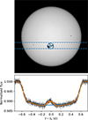 |
Fig. 1. Top: The Sun during its activity maximum in 2014. The transit path of Jupiter in front of solar latitude −17.5° is marked with dashed lines. The largest sunspot group of the solar cycle, AR2191 is close to the centre of the transit path. The properties of the spot group were reconstructed based on the simulated transit light curve of Jupiter. The inner blue circle indicates the position and size of the dark region, if the beginning and end of the eclipse over the spot group are taken as tin and tout, respectively. The outer circle represents the spot group if the eclipse times are adjusted to tin − σDR and tout + σDR. Below: Simulated transit light curve of Jupiter, in front of −17.5° solar latitude. The light curve has similar noise properties as high precision TESS observations. A model assuming one dark region (orange) and an unspotted photosphere (blue) is shown on top of the light curve. |
This simulation shows that the temperature of the eclipsed region and coverage estimated using transit mapping, may differ considerably from reality. Thus, when we refer to the temperatures of eclipsed regions in this study, it is actually a weighted mean temperature representing the whole active region covered by the transit. This also refers to the spot coverage: rather than representing the total umbral area, it refers to the whole active region, for which the temperature is estimated.
3.5. False positives
The posterior samplings and model comparisons probably yield robust results. However, they are not infallible. If in some cases, complex correlated variation is present in the observations, it may get mistaken for an eclipse signal over a DR. Therefore, it is necessary to have some safeguards to ensure that the identified signal comes from a DR eclipse. Astrophysical and instrumental false positives can also mimic signals from DR occultations. For this reason, we tested whether the flux variations, identified as DR eclipses have other origins, by performing a series of tests for false positives.
Although small-scale brightness variations on the stellar surface, or simply correlated noise, can give rise to false positives, the brightness modulations identified as eclipses over DRs, can also be caused by some unknown, unrelated astrophysical source. Yet, in such a case, similar modulations in flux would also be present in the time-series outside the transit events. We tested this possibility for the stars that showed strong evidence for DR occultations, by extracting N = 50 randomly selected subsets from their light curves when no planetary transit occur and by searching those out-of-transit subsets for signals described in Eq. (1).
Flares that occur during the planetary transit may cause variations similar in amplitude and timescale to eclipses over DRs. It is important to note that the planet is not expected to transit the flaring region for such an event. We aimed to estimate the expected duration of flare signals that could, in principle, appear in our data. To do this, we used the t1/2 timescales of flares observed in TESS stars with effective temperatures below 5200 K, as reported by Seli et al. (2025). We estimate that for flares with amplitudes Af < δ, the signal would drop below the typical noise level of the observations after approximately 4 t1/2, which corresponds to  seconds. A significant fraction of DR occultations in our sample (44.4% of those listed in Table 3 and 25.3% of those in Table D.1 in Appendix D) fall within this one-sigma interval, demonstrating the need to compare these signals with flare models.
Significance and properties of candidate DR eclipse events identified in this analysis.
Distinguishing between the planet transiting over a dark region, and a flare happening anywhere on the stellar surface is a relatively straightforward task, as flares follow distinct asymmetric morphologies (Howard & MacGregor 2022), whereas DR eclipses are expected to be more symmetric. We tested the possibility that the brightness variations identified as DR eclipses may be due to flares by sampling a simple flare model on the transit light curves with DR detections. Our flare model consisted of a discontinuity at time tf, such that the flux jumps above the baseline, followed by an exponential decay. At time ti the flux is modulated by the flare as
 (8)
(8)
where Af is the amplitude of the flare at peak time tf, and τ is the timescale of the exponential decay. A planetary transit model with a co-occurring flare is then of shape
 (9)
(9)
where ftr is the flux from the reference model and ϵi is the Gaussian noise term (see Eq. (2)). We rejected eclipse candidates after visual inspection and if the Bayes factor of the flare model in favour of the DR model indicated a strong evidence of a flare signal.
The pre-search data conditioning pipeline of the Kepler and TESS telescopes may introduce artefacts to the observations on similar timescales as DR eclipses. To ensure that the identified eclipse signals are not artefacts from the pipeline, we sampled the SAP light curves for DR eclipses, where such events were found.
Light curves on longer timescales also provide some additional means for testing the nature of the signals interpreted as occultation events. Assuming that the DRs identified from eclipses are non-axisymmetric with respect to the stellar axis of spin, we expect that they leave a photometric signal in the light curve of the star as they co-rotate with the stellar surface. The maximum flux deficit a dark region with contrast c and radius rDR can leave in the light curve of the star is (Tregloan-Reed & Unda-Sanzana 2019)
 (10)
(10)
This approach gives an upper limit for photometric variations on the timescale of the stellar rotation, induced by the co-rotating DR. If the expected signal is above the noise limit for rotational modulation, but cannot be identified in longer baseline observations, the in-transit flux variation may have some other origin than an eclipse over a dark region.
3.6. Average number of dark regions and spot filling factor
The average number of dark active regions on a star can be approximated, assuming a uniform distribution of DRs, by taking the occurrence rate of eclipses over DRs and the size of the segment on the star that is transited by the planet. This is a very crude approximation, which assumes a uniform latitude distribution of dark regions, and it does not, for example, accurately reflect the Sun’s spot distribution.
Let us take the radius of a star to be unity and let us denote the average number of dark active regions on the stellar surface as Ns. At any time, we see half of the stellar surface, so the average number of DRs on the visible hemisphere is NDR/2.
As the planet transits the stellar hemisphere, the area of the transited band on the stellar surface, without stellar rotation, is
 (11)
(11)
where h = min(b + r, 1)−max(b − r, −1), and b = sin α is the impact parameter. We note that Atr is half the surface area of a spherical segment of height h. The number of transited dark regions is obtained by dividing the transited area by the surface area of the visible hemisphere, and multiplying it by the number of dark regions on the visible hemisphere
 (12)
(12)
However, assuming that the centres of some active regions are not transited by the planet (grazing transits), the size of the band where active regions may be eclipsed widens on both sides by the radius of the active region rDR, and the number of eclipsed dark regions is described by
 (13)
(13)
This is a valid consideration, as we find that the apparent radii of the eclipsed dark regions are often larger than the apparent radius of the planet. It follows from this calculation, that the average number of DRs is not necessarily an integer. Fig. 2 shows the geometry of the transit. In summary, the mean number of DRs for the star is calculated by dividing the number of detected DR eclipse candidates by the number of analysed transits, and multiplying that result with the inverse ratio of the area of the band from where DRs may be transited by the planet to the area of the full stellar surface.
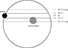 |
Fig. 2. Geometry of a planetary transit across a star. The planet of radius r transits the star at impact parameter b. The band transited by the planet is marked by dashed lines. Active regions with radii rDR and centres located within the band outlined by dotted lines may be eclipsed by the planet. |
The spot filling factor of the star, fS, can be approximated by multiplying the average number of dark regions with the mean area of dark regions and dividing it with the area of the stellar surface. This approximation is valid even if there is no spin-orbit alignment, and the inclination of the star is not 90°.
4. Results
After analysing 3273 light curves containing transit events of 99 planets from the Kepler, K2, and TESS missions, we found six targets that show strong evidence for eclipse events over dark regions during the transits. In total, we identified 102 such candidate eclipses.
In Fig. 3, we show the sample of analysed exoplanets on the stellar effective temperature–stellar radius plane. The scaling of the filled circles corresponds to the planet–star radius ratios. Targets for which DR eclipses were identified are marked in colours. The colouring corresponds to the Gaia magnitudes mGaia. As stellar brightness correlates with the photon counts and the noise levels of the observations, brighter stars are expected to show more occultations of DRs than fainter ones. Grey dots mark the planets where no DR eclipses were identified. All but one star with a DR eclipse candidate was of K spectral class.
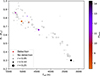 |
Fig. 3. Distribution of systems with DR eclipse detections (coloured dots) in terms of stellar effective temperature Teff, stellar radius R*, and planet–star radius ratio r, compared to systems where no DR eclipse was found (grey dots). The colour mapping of the systems with DR eclipses corresponds to the Gaia magnitudes mGaia of the stars. |
In Table 3, we provide detailed information about each planetary transit (except for those of HAT-P-11 b, see Sect. 4.1) during which a candidate DR eclipse occurred. We list the planet’s name, the index and the mid-time (tc) of the transit, the significance of the DR eclipses expressed as the logarithm of the likelihood ratio (log l) between the DR model and the reference model, and the Bayes factors between the two models (B1, 0). Additionally, four parameters characterising the DR eclipses are reported: the length of the eclipse (tlen = tout − tin + 2σDR), the mid-time of the DR eclipse relative to the time of conjunction of the planetary eclipse (tmid), the minimum angular size of the eclipsed region (rmin), and the contrast of the eclipsed region (c).
4.1. HAT-P-11
HAT-P-11 is a  solar mass, K4V spectral type star with an effective temperature of 4780 ± 50 K. It is transited by one planet, HAT-P-11 b, a super-Neptune on a 4.89-day orbit (Bakos et al. 2010). Occultations of dark regions by the planet have been found in its transit light curves soon after its discovery (Sanchis-Ojeda & Winn 2011). Another planet in the system was detected from radial velocity measurements on a ∼3400 d orbit (Yee et al. 2018). The star was observed by Kepler in its original mission, and then by TESS over six sectors. Its relatively high brightness (V = 9.46) makes it an ideal target for monitoring with both instruments.
Bakos et al. (2010) found significant flux variations in the observations of HAT-P-11, with a period of P = 29.2 d, which they attribute to the rotational period of the star. Age estimates for the star range between  Gyr (Morton et al. 2016) and
  Gyr (Bakos et al. 2010). From measuring the Rossiter-McLaughlin effect, Winn et al. (2010) estimated a sky-projected obliquity of
  degrees for the system.
We analysed 214 transits of HAT-P-11 b, 183 recorded by Kepler, and 31 recorded by TESS. We identified 85 possible DR occultation events by HAT-P-11 b, all of them observed by Kepler. This planet alone has more DR candidates than all other planets in our sample combined, and we list these candidates in Table D.1 of Appendix D. The planet was also the only one in our sample that showed multiple DR eclipses during a single transit.
We found extreme variations around some transit events in the PDC light curves as artefacts from the Kepler Pre-search Data conditioning Pipeline. These variations complicated the normalisation of certain transit light curves, forcing us to exclude some light curves from our sample. Accounting for these variations is outside the scope of the current work. For this reason, we advise caution when interpreting the statistics of HAT-P-11 b, and suggest that the number of identified DRs provides a lower limit to the number of identifiable occultation events in the sample.
The contrasts of the eclipsed active regions were between  and
and  . Adopting the effective temperature estimate of 4780 ± 50 K (Bakos et al. 2010), we calculate that the mean temperature of the darkest transited region was ΔT ≈ 950 K cooler than the unspotted photosphere.
4.2. HD 189733
HD 189733 is the brightest star (mGaia = 7.41) for which we detected DR eclipse candidates. The star is of spectral type K2V (Gray et al. 2003) and has an effective temperature of Teff = 5050 ± 50 K (Bouchy et al. 2005). It is the main component of a binary system, where the projected separation of the two components is about 216 AU (Bakos et al. 2006). The star is known to be orbited by one planet, a hot Jupiter with an orbital period of P = 2.22 d. The planetary orbit has an inclination angle i = 85.5° with a low mutual inclination angle λ = −0.85° (Triaud et al. 2009).
Bonomo et al. (2017) estimated a stellar rotation period of 11.95 ± 0.01 d from ground-based photometric observations. Age estimates for this star range from less than 1 Gyr (Ghezzi et al. 2010) to  Gyr (Torres et al. 2008). The star is known to show signals of relatively high stellar activity. Wright et al. (2004) measured a chromospheric activity index of S = 0.525, while Barnes et al. (2016) reported log R′HK indices between −4.55 and −4.50. Both statistics imply increased magnetic activity, which would favour a younger age.
The system has exhibited one of the early examples of eclipses of dark regions by an exoplanet. Pont et al. (2007) found two such events while monitoring three transits of the planet with the Hubble Space Telescope (HST). Later, Sing et al. (2011) found similar eclipse signals in repeated HST observations, and, through stellar atmospheric modelling, estimated the spot temperatures to be around 4250 K.
Recently, upon analysing archival spectra from HST observations, Narrett et al. (2024) inferred the spot-covering fraction and the effective temperature of the spots for HD 189733. They found spot covering fractions between 38%±4% and 47%±3% for spectra taken at different times, and a spot effective temperature of  K.
K.
The target was observed by TESS in Sectors 41 and 54. We analysed the 21 transits recorded by TESS and detected eight new DR eclipses in the transits of HD 189733 b. After comparing the DR eclipse signals with the simple flare model, described in Section 3.5, we rejected one detection (transit 2324). Fig. 4 shows an example transit light curve of HD 189733 b with one DR eclipse, shortly before the centre of the planetary transit.
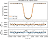 |
Fig. 4. Transit of HD 189733 b observed by TESS with a cadence of 120 s. Black dots represent the mean of consecutive subsets of ten observations. Maximum likelihood fits from the nDR = 1 and nDR = 0 models are marked with orange and blue lines respectively, one sigma uncertainties are marked as shaded areas. The residuals of the highest likelihood nDR = 1 and nDR = 0 model fits are shown in the middle and the bottom of the figure, respectively. The feature between t − tc ≈ −2200 s and t − tc ≈ −300 s is an eclipse of a dark region with a radius of |

The contrasts of the eclipsed regions we detected are relatively low, ranging from  to
to  . The detection of such low contrast eclipses was possible due to the high signal-to-noise ratio (Str = 57.3) of the observations. The contrast of the darkest eclipsed region corresponds to an effective temperature difference of ΔT ≈ 120 K, when taking 5050 ± 50 K as the effective temperature of the star (Bouchy et al. 2005). This, however, does not strictly correspond to the temperature difference of the photosphere and the spot umbra itself, as the temperature difference estimate is based on the weighted mean effective temperature of the entire eclipsed region, which may include unspotted areas or even bright faculae.
The durations of DR eclipses were between ∼930 s and ∼4410 s, and the minimum radii of the eclipsed regions ranged from  degrees to
  degrees. These properties are consistent with earlier HST observations by Pont et al. (2007). We estimate an average number of dark regions of NDR = 3.79, which, with the maximum DR radius of the sample gives a spot filling factor of 13%.
When assessing the frequency of astrophysical false positives, we found one out-of-transit light curve with strong evidence for a signal resembling DR eclipse. This is possibly due to the elevated activity of the star, and in our view does not invalidate the DR eclipses found during the planetary transits, due to their vastly differing occurrence frequencies during and outside of transit.
Analysing the transit observations previously published, Baluev (2022) reported transit timing variations for HD 189733 b of the order of ∼70 s. Their analysis suggests that only ∼10 s of these variations can be attributed to the planet transiting in front of an uneven photospheric brightness field. We find a maximum transit mid-time difference of Δtc ∼ 30 s in the TESS observations. The largest discrepancy in transit mid-times between the nDR = 0 and nDR = 1 models was ∼20 s.
4.3. Kepler-411
Kepler-411 is a K2V spectral type star of 0.87 ± 0.04 solar masses and the age of 212 ± 31 Myr (Sun et al. 2019). The star is orbited by four planets, of which three transit. The inclination of the star is 89.79 ± 0.19° (Tuomi et al. 2025).
The star is well known for its activity and eclipses of dark regions from its planets. Araújo & Valio (2021) studied the star extensively in terms of DR eclipses. Their detection criteria for an eclipse was that the amplitude of variations from the reference model exceed 3σ and reported nearly two hundred DR eclipses in the Kepler time-series.
Recently, Tuomi et al. (2025) studied the star in terms of signatures of DRs. They sampled the transit light curves of planet c for DR eclipses and performed rotational modelling to characterise DR geometries for the whole stellar surface. They applied the same detection criteria in their analysis as applied in the current work and reported three DR eclipse events from planet c, all within a 50 d long interval.
The star is in the original Kepler field and was observed in several TESS Sectors. The noise levels of the TESS observations were too high to enable robust DR detections. We therefore searched the Kepler data for DR occultation events in the transits of all the planets but managed to detect DR eclipses only for the transits of planet c. This may be explained by the lower number of transits from the other planets, the shallowness of their transits, or the DRs being constrained to the latitude band coinciding with the orbital inclination of the planet c.
After comparing the DR signals to the simple flare model, we rejected one eclipse detection over a dark region (transit 164). Our DR detections are broadly consistent with those of Tuomi et al. (2025), although the spot candidate in transit 116 did not achieve a likelihood ratio high enough to exceed our corrected FAP thresholds adjusted for npeaks. We could not replicate most DR detections of Araújo & Valio (2021), probably due to adopting a rather conservative set of detection criteria.
4.4. TOI-1268
TOI-1268 is a young, K1–K2 V spectral type main sequence star, with an estimated age of 245 ± 135 Myr (Dong et al. 2022). It has a Gaia magnitude of mGaia = 10.69 and a TESS magnitude of mTESS = 10.15. The TESS transit observations have a mean Str of 6.17. The star’s rotation period is 10.8 days (Dong et al. 2022). TOI-1268 is orbited by a known planet (TOI-1268 b) with a mass comparable to Saturn. The planet has an orbital period of Porb = 8.16 days (Šubjak et al. 2022). Measurements of the Rossiter–McLaughlin effect by Dong et al. (2022) indicate that the star and its planet are in spin–orbit alignment.
We analysed 14 transits of the planet, observed over five TESS Sectors. We obtained decisive evidence for one DR eclipse (log10B = 5.34), during transit 3 of the planet. The transit light curve with the residuals from the DR occultation- and the reference models is shown on Fig. 5.
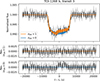 |
Fig. 5. Transit of TOI-1268 b observed by TESS with a cadence of 120 s. The DR eclipse occurs between t − tc ≈ −1100 s and t − tc ≈ 4200 s. The eclipsed region has a minimal radius of |

The minimal radius of the eclipsed dark region is  °, while its contrast is
  . This radius is towards the higher end of the DR radius distribution reported in this work, and is the largest DR radius for a star with non-axisymmetric signals. Taking the effective temperature of the star to be 5257 ± 40 K (Dong et al. 2022), we obtain a mean effective temperature of the eclipsed active region as 5031 ± 40 K. We note that the Bayesian analysis indicated that the flare model has strong evidence in favour of the DR model (B = 31.1), but after the visual inspection of the signal, we find it unlikely that the brightening during the transit was caused by a flare.
Based on visual inspection of the eclipse signal it may appear credible that the signal originates from two separate DRs. However, the sampling of a model with nDR = 2 did not provide strong evidence for the presence of two distinct DRs.
4.5. TOI-3884
TOI-3884 is an M4 spectral class star, transited by one planet with an orbital period of P = 4.54 d, on a supposedly highly misaligned (ψ = 50 ± 12°) orbit (Almenara et al. 2022). Rotation period estimates for TOI-3884 range between Prot = 4.22 ± 1.09 d (Libby-Roberts et al. 2023) and Prot ≈ 18 d (Almenara et al. 2022). Both estimates rely on the rotational broadening of lines in the star’s spectra, since no rotational modulation can be observed in the light curve of the star. The former value would, in practice, suggest a synchronous orbit for the planet. The estimated short rotation period suggests the star is reasonably young.
The star was observed by TESS with a cadence of 120 s in two consecutive sectors, during which eight transits of TOI-3884 b were recorded. Shortly after each transit began, the light curve was modulated with a feature similar to what a DR occultation would cause. Based on TESS measurements, and observations taken with a 1-m telescope at Teide observatory with the Las Cumbres Observatory Global Telescope (LCOGT), Almenara et al. (2022) interpreted that the modulation is caused by a giant polar dark region of radius r = 49° (17% of the surface covered). Subsequent ground-based observations of Libby-Roberts et al. (2023) confirmed the existence of the dark region.
We performed our analysis on the eight transits recorded by TESS and found evidence for three DR eclipses. We found that the model with one DR was strongly favoured against the reference model for two transits (B = 131.3, B = 50.1 for transits −16 and 1, respectively). We also found one transit for which the DR occultation model had decisive evidence against the reference model (B = 185.7 for transit −15).
We note that we obtained solutions that remained reasonably similar between transits ( deg,
deg,  , on average for the eight transits). This suggests that the varying detection statistics are probably an artefact of the high noise levels of TESS observations.
4.6. WASP-107
WASP-107 is a K6V spectral type star. It is orbited by two planets, of which one is transiting (Anderson et al. 2017). WASP-107 b orbits its star with a 5.72 d period. Using Rossiter–McLaughlin measurements, Rubenzahl et al. (2021) found that WASP-107 b has a retrograde, polar orbit, with a projected spin-orbit angle of  °.
°.
WASP-107 has a V-band brightness of 11.47. It was observed in one K2 campaign with 60 s cadence with a high signal-to-noise ratio (Str = 35.7). Eclipses of DRs have been reported for this star by several authors with differing criteria for detection. The star has not been observed by TESS with a sufficiently high cadence that would allow the detection of such eclipses.
Močnik et al. (2017) inspected the residuals of the transit light curves of WASP-107 b, after the best-fitting MCMC transit model had been subtracted. They inspected the residuals by eye and categorised them as definite and possible occultation events. They found five definite and four possible DR occultations. Dai & Winn (2017) found three DR eclipses (which they called “visually obvious”) in the same K2 observations. Their eclipse model was of a simple Gaussian curve, and they demanded that the ΔBIC > 10 in favour of the DR model, as detection criteria. Both Močnik et al. (2017) and Dai & Winn (2017) note that the star and the planet are not in spin–orbit alignment.
After analysing nine transits recorded by K2, we identified three potential DR eclipses in the transits of WASP-107 b. The DRs had contrasts between  and
and  , and minimal radii ranging from
  degrees to
  degrees. Notably, the first two of the three eclipsed regions were smaller and had higher contrasts compared to the third, implying that the last eclipsed feature is warmer and more diffuse than the first two. The DRs identified by us correspond to those identified by Dai & Winn (2017).
Adopting a stellar effective temperature of 4430 ± 120 K (Anderson et al. 2017), the contrasts indicate that the effective temperatures of the eclipsed regions range from 4235 ± 110 K to 4413 ± 119 K. We estimate the average number of dark regions on the star to be 3.73 and the upper limit for the spot filling factor to be 11%.
5. Discussion
The DR eclipse modelling and significance assessment was performed following a Bayesian framework common in related fields of astrophysics. The criteria for confirming a more complex model were more conservative than those used by most authors. For this reason, we detected fewer DRs for several stars with published detections. This is particularly clear for Kepler-411 (see also Tuomi et al. 2025), for example, but we also failed to detect the reported DR eclipses of Zaleski et al. (2020) for Kepler-45 b. This does not imply that the corresponding DR detections reported earlier were false positive detections, but it does cast doubt on their statistical significance.
Detected DR eclipse durations range from ∼200 s to ∼5300 s. As shown by Silva-Valio et al. (2010), DRs closer to the central meridian are more detectable than those on the stellar limbs. This is due to distortion effects, as the transit light curve becomes steeper as the planet transits in front of regions closer to the stellar limb. We found 90% of DR candidates within 22.4° of the meridian, with none beyond 46.9°.
For planets with smaller angular radii than that of the transited dark regions, the contrast did not exceed 0.43, while the same number was 0.69 for smaller features, where the contrast was corrected following Eq. (4). If the contrast of the dark region is c ≲ 0.1, one-sigma errors for the stellar dark region and unspotted surface temperatures overlap. The dark region’s effective temperature is derived from the stellar surface temperature and the contrast of the eclipsed region, with the errors propagating accordingly. The real temperature difference between individual spots and the photosphere may be an order of magnitude higher than inferred from the eclipsed region contrast (see Appendix C).
We compared our definition of eclipse length tlen with an alternative definition, tlen′=tout − tin, and the corresponding inferred rmin′. We calculated rmin′ for the candidate eclipses in our sample and present the comparison between rmin and rmin′ in Fig. 6. In this figure, dark regions of HAT-P-11 are marked in orange, while features from all other stars are marked in blue. A simple linear regression fit to the rmin and rmin′ values revealed a slope of β = 0.72, indicating a systematic relationship between the two definitions.
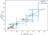 |
Fig. 6. Comparison of dark region radii when calculated based on eclipse lengths tlen = tout − tin + 2σDR (rmin) and tlen′=tout − tin (rmin′). A linear trend, marked with a dotted black line, was fitted to the dataset, with the linear fitting yielding a slope of β = 0.72. |
Empirical models predict lower spot temperatures than our estimates for eclipsed active regions. One such model was derived by Berdyugina (2005). To estimate spot temperatures in their sample, they used several methods, including Doppler imaging, light curve modelling, molecular bands, and atomic line-depth ratios. Herbst et al. (2021) updated this empirical relation upon extending the original sample of Berdyugina (2005). As an example, for HD 189733, Eq. (6) of Herbst et al. (2021) predicts a temperature difference of ΔT = 578 ± 467 K between the umbra and the unspotted photosphere, which is a factor of five bigger than the maximum temperature difference calculated from the contrast of an active region (ΔT ≈ 120 K). However, both Berdyugina (2005) and Herbst et al. (2021) advise using their relations with caution, since for instance, they cannot reproduce the solar spot temperature contrasts.
All planets with candidate DR occultations had orbital periods shorter than 9 days. These planets have relatively large radii compared to their stars, ranging from 0.045 to 0.18. The signal-to-noise ratio distribution of the transit light curves for planets with DR eclipse detections and those without were reasonably similar.
Of the 89 stars in our sample, 80 had age estimates and 41 had rotation periods listed in the NASA Exoplanet Archive, with 38 having both. Since the archive may lack some published values, we reviewed the literature for stars with DR eclipse candidates. Of the six such planets, five had age estimates and all six had rotation periods. Two stars with DR eclipse candidates are younger than 1 Gyr (Kepler-411 and TOI-1268, 212 ± 31 Myr and 245 ± 135 Myr, respectively), both have ∼10 d rotational periods. Fig. 7 compares the ages and rotation periods of the stars with DR eclipse candidates and those where no eclipse signals were found in the analysis. The figure only shows those stars whose ages and rotation periods were derived simultaneously. Different measurements for the same star are connected by dashed lines.
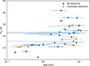 |
Fig. 7. Comparison of ages and rotation periods of the stars with DR eclipse candidates (orange) and stars where no DR eclipse was detected in our analysis (blue). |
It is worth comparing the scale of the transited features with the resolution of other methods to resolve the surfaces of late-type stars. One common method for recovering the brightness distribution of late-type stars is Doppler imaging, which relies on a time-series of spectroscopic measurements of a star (see e.g. Piskunov et al. 1990). Coupled with polarimetric measurements, the large scale magnetic field topology of the star may also be recovered, which can serve as a basis for the reconstruction of the surface brightness distribution. Depending on the phase coverage and the projected rotational velocity (v sin i), these methods can reveal surface details as small as 5 degrees (Carroll et al. 2012).
While Doppler imaging is limited in resolution due to requirements on stellar rotational velocity, and the resolution and signal-to-noise ratio of the spectra, transit mapping has a higher potential to discern the smallest dark features of the stellar surface. We found that the main limiting factor for the detection of small dark regions is the signal-to-noise ratio of the data. The smallest DR in our sample had a radius of 1.6 degrees (HAT-P-11). Inverse photometric modelling of rotational signals may discern dark features on similar size scales, but fails to recover the contrasts of DRs. A small, high contrast region would produce a similar signal as a larger, low contrast region (see e.g. Tuomi et al. 2025).
Our sample contained 8 K-dwarfs and 4 M-dwarfs observed by the Kepler or K2 missions, and 54 K-dwarfs and 24 M-dwarfs observed by TESS. Kepler and TESS both provided light curves for the candidate DR occultation detections of three stars (Kepler: HAT-P-11, Kepler-411, and WASP-107, TESS: HD 189733, TOI-1268, and TOI-3884). Of the stars with candidate DR eclipses, only TOI-3884 was an M-dwarf, while the rest were K-dwarfs.
The spot detection frequency of Kepler was 37.5% for K-dwarfs, while for TESS, it was 3.7% and 4.2%, for K- and M-dwarfs, respectively. Using a set of simulated TESS light curves, Tregloan-Reed & Unda-Sanzana (2021) predicted that spot detection frequencies for K- and M-dwarfs in the TESS sample would be 10.66%±0.41% and 17.26%±0.48%, respectively. The difference between their results and those presented in this analysis may be due to the detection criteria they applied. The authors compared flux deficits to the root mean square scatter without considering event length or phase. With TESS expected to find 1700 planets (Sullivan et al. 2015), a larger sample is needed for more robust spot detection statistics.
Photometric variations during transits could, in theory, originate from exomoons transiting the disk of their planets. To test this, we calculated the minimum duration of an exomoon transit in front of the disk of its planet. Following Dobos et al. (2021), we approximate the semi-major axis of the innermost stable orbit of a moon as 2Rp with circular orbits. For planets with DR eclipse candidates, predicted exomoon transit durations range from ∼3230 s (HAT-P-11 b) to ∼15 000 s (WASP-107 b). Only one DR eclipse candidate (HAT-P-11 b, transit −369) exceeded this threshold. Additionally, planets with multiple DR eclipses show varying signal amplitudes, which is impossible from exomoon transits.
We estimated the β factor for each target with a candidate detection, following the method described by von Essen et al. (2020). The analysis was performed on the set of out-of-transit light curves described in Section 3.5. We computed the β factor over timescales corresponding to the durations of our candidate occultation signals over dark regions. Table 4 presents the minimum and maximum timescales (tmin and tmax) considered, along with the maximum β-value observed within this interval. The contribution of correlated noise in the total noise of observations remained reasonably low on the investigated time scales. Even for the star with the highest beta factor in this sample, the correlated noise is much weaker than the signal required from eclipse candidates over dark regions.
β factors for the stars in our sample with a candidate eclipse over a dark region.
Another systematic search for DR occultations was conducted by Baluev et al. (2021). They analysed spot- and facula-induced modulations in 1598 transit light curves from 26 targets, collected through a network of amateur and professional observatories. Their DR eclipse model was a simple Gaussian profile, corresponding to the extreme case of tin = tout in our Eq. (1). They applied an iterative algorithm to detect Gaussian anomalies, retaining only statistically significant and well-justified features. Overall, they reported 38 potential occultations of dark regions.
Our DR contrast results align reasonably with most of Baluev et al. (2021). However, due to their definition of occultation length (the σ of the Gaussian anomaly), their occultations occur on a shorter timescale than those identified in this analysis. Multiplying their occultation lengths by a factor of 2 reduces these differences, but several of our candidate eclipses still occur on longer timescales compared to those of Baluev et al. (2021), even after the adjustment.
Baluev et al. (2021) reported DR eclipse detections for 20 of 26 stars, while we found occultation candidates for 6 of 89 stars. This results in a detection rate 11 times higher in their study (76.9%) compared to ours (6.7%). Among the 5 stars analysed in both studies (HAT-P-12, HD 189733, Qatar-4, TrES-1, and WASP-2), we identified candidate occultation events only for HD 189733. Several factors may explain the differences in detection statistics between the two studies. Firstly, none of the observations of Baluev et al. (2021) were conducted using the space telescopes employed in our study. Secondly, improper normalisation of some out-of-transit light curve segments in their dataset could have introduced artefacts into the transit signals. These artefacts might cause deviations from the quadratic limb-darkening law assumed in their analysis, resulting in the appearance of DR-like features. Furthermore, the dataset of Baluev et al. (2021) includes DR occultations occurring during the ingress or egress phases of transits. While such events are also allowed in our analysis, due to their lower expected amplitudes, they are unlikely to be confirmed by our detection criteria.
Only two objects, HAT-P-11 b and HD 189733 b, had more than three DR occultation candidates in our sample. Fig. 8 compares the durations of DR occultation events and contrasts of the eclipsed regions for these two planets. The eclipsed dark regions on HAT-P-11 are generally smaller and darker compared to those on HD 189733. This difference in DR properties may be attributed to different planet-star radius ratios and orbital alignments. The radius ratios for HAT-P-11 b and HD 189733 b are r = 0.06 and r = 0.15, respectively. HAT-P-11 b, being smaller, can completely overlap with individual dark regions on the stellar surface, while the larger HD 189733 b may cover both bright and dark regions, reducing the contrast of the observed signal. Additionally, HAT-P-11 b is orbitally misaligned, allowing it to cover a wide range of stellar latitudes. No such misalignment is observed for HD 189733 b. If active regions are spread longitudinally on these stars, HAT-P-11 b would briefly transit these regions, while HD 189733 b would cover the same latitudes throughout its transit.
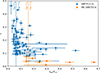 |
Fig. 8. Relative durations tlen/T14 and contrasts c of dark region occultation candidates are shown for the two planets with the most events. Dashed vertical lines represent durations where the angular radius of the dark regions rDR matches that of the planet rp. For durations below this threshold, the contrasts have been adjusted using Eq. (4). |
We found that by far the most false positives came from the varying transit depth from stars with low signal-to-noise observations. Outlying flux observations may also cause high enough Bayes factors for DR detections. Both these cases can be easily refuted with visual inspection.
The frequency of DR eclipses in a planet’s transits allows us to estimate the mean number of dark regions NDR. Combined with DR sizes, we may estimate the range of possible spot filling factors fS of each star. Table 5 lists the mean DR numbers, and the range of spot filling factors [fS, min, fS, max] for each star where a DR eclipse candidate was found in our sample. Spot filling factors are derived from the fractional angular areas of the smallest and largest eclipsed DRs, multiplied by the mean number of DRs. The DR numbers and spot filling factors are approximated with the assumption that the DRs are distributed uniformly on the stellar surface. At least for TOI-3884, we have good reason to believe that this does not hold, as its planet is probably repeatedly eclipsing the dark polar region of the star. Our analysis also failed to pick up numerous eclipse events of the same region, due to the noisiness of the data. Because of this, we advise caution when handling the spot occurrence statistics of this star.
Number of analysed transits ntr, mean numbers of dark regions NS, and the range of possible spot covering fractions [fS, min, fS, max].
The upper limits for spot filling factors we observed for the stars range between 0.6% and 16.9%. For every star in our sample, the spot filling factors have remained at least a factor of two lower than what is inferred for young K- and M-dwarfs based on studies of TiO absorption bands (O’Neal et al. 2004). This discrepancy may arise because transit mapping is more sensitive to the stellar centre or because smaller, lower-contrast regions remain undetected because of observational noise.
We calculated the maximum brightness variation each DR could induce per stellar rotation and compared it with flux variations around transit events where DRs were detected. We extracted the observations in a 30 d window centred around the DR eclipse event, and smoothened the observations by taking the running mean of every 20th flux measurement for 120 s observations, and every 40th flux measurement for 60 s observations. Flares were omitted from the data after visual vetting. We used SAP fluxes for this comparison, unless they were contaminated by instrumental drift. We preferred SAP fluxes to PDSCAP fluxes due to the fact that stellar variability over timescales longer than around 10 days may get significantly dampened by the data conditioning pipeline (see e.g. Gilliland et al. 2015). Table 6 compares the amplitude of brightness variations Aphot in the Kepler and TESS observations around each DR occultation candidate and the maximum possible flux change ΔFDR the dark region can cause on the star. This comparison is presented separately for the DR candidates of HAT-P-11 b, in Table D.2 of Appendix D. The estimated flux variations from all non-axisymmetric DRs in our sample were consistent with the observed flux changes over the stellar rotation.
Expected maximum flux change from co-rotating starspots ΔFDR compared to the amplitude of the rotational modulation observed around the transit Aphot in SAP or PDC light curves.
6. Conclusions
We performed a uniform analysis of possible occultations of dark regions by exoplanets in the Kepler and TESS high cadence observations of K- and M-dwarfs. We analysed 3273 transits from 99 planets in total, and found strong evidence for DR eclipses on 102 occasions, by 6 planets.
We report new DR eclipse candidates for HD 189733 b in recent TESS data, confirming past HST detections (Pont et al. 2007; Sing et al. 2011), and an individual candidate for TOI-1268 b. Our analysis supports previous detections for HAT-P-11 b (Morris et al. 2017) and WASP-107 b (Dai & Winn 2017) and recovers some DR eclipses from Kepler-411 c (Araújo & Valio 2021) and TOI-3884 b (Almenara et al. 2022; Libby-Roberts et al. 2023). Differences in detection criteria and noise treatment likely explain some non-detections.
The candidate eclipse durations range from approximately 200–5300 seconds, with minimum radii of the dark regions spanning 1.6° to 29.5°. Kepler’s spot detection frequency for K-dwarfs was 37.5%, while for TESS, it was 3.7% and 4.2% for K- and M-dwarfs, respectively. The observed upper limits for spot filling factors range from 0.6% to 16.9%.
In this work, we have introduced a new modelling framework to analyse large quantities of planetary transit observations, aimed at building robust DR statistics. As the number of known exoplanets around late-type stars is expected to grow, the likelihood of detecting DR occultation events will also increase. In the process, we will eventually get reliable statistics of the smallest detectable DRs on other stars, and, potentially improve the assumptions and understanding of the magnetic activity of late-type stars.
https://exoplanetarchive.ipac.caltech.edu/, accessed on July 11, 2023.
The central wavelength of Kepler and TESS telescopes are 640 nm and 786.5 nm, respectively.
Acknowledgments
We are thankful to the anonymous referee and to Katalin Oláh for valuable feedback. AH and MT gratefully acknowledge support from the Jenny and Antti Wihuri Foundation. The authors acknowledge the Research Council of Finland project SOLSTICE (decision No. 324161). The authors wish to acknowledge CSC – IT Center for Science, Finland, for computational resources and support. This research has made use of NASA’s Astrophysics Data System. This research has made use of adstex (https://github.com/yymao/adstex).
References
- Addison, B., Wright, D. J., Wittenmyer, R. A., et al. 2019, PASP, 131, 115003 [NASA ADS] [CrossRef] [Google Scholar]
- Akeson, R. L., Chen, X., Ciardi, D., et al. 2013, PASP, 125, 989 [Google Scholar]
- Almenara, J. M., Bonfils, X., Forveille, T., et al. 2022, A&A, 667, L11 [NASA ADS] [CrossRef] [EDP Sciences] [Google Scholar]
- Alsubai, K., Mislis, D., Tsvetanov, Z. I., et al. 2017, AJ, 153, 200 [Google Scholar]
- Alsubai, K., Tsvetanov, Z. I., Latham, D. W., et al. 2018, AJ, 155, 52 [Google Scholar]
- Alsubai, K., Tsvetanov, Z. I., Pyrzas, S., et al. 2019, AJ, 157, 224 [NASA ADS] [CrossRef] [Google Scholar]
- Anderson, D. R., Collier Cameron, A., Gillon, M., et al. 2012, MNRAS, 422, 1988 [Google Scholar]
- Anderson, D. R., Collier Cameron, A., Delrez, L., et al. 2014, MNRAS, 445, 1114 [NASA ADS] [CrossRef] [Google Scholar]
- Anderson, D. R., Collier Cameron, A., Delrez, L., et al. 2017, A&A, 604, A110 [NASA ADS] [CrossRef] [EDP Sciences] [Google Scholar]
- Araújo, A., & Valio, A. 2021, ApJ, 907, L5 [CrossRef] [Google Scholar]
- Artigau, É., Hébrard, G., Cadieux, C., et al. 2021, AJ, 162, 144 [NASA ADS] [CrossRef] [Google Scholar]
- Awiphan, S., Kerins, E., Pichadee, S., et al. 2016, MNRAS, 463, 2574 [NASA ADS] [CrossRef] [Google Scholar]
- Baglin, A., Auvergne, M., Boisnard, L., et al. 2006, 36th COSPAR Scientific Assembly, 36, 3749 [Google Scholar]
- Bakos, G. Á., Pál, A., Latham, D. W., Noyes, R. W., & Stefanik, R. P. 2006, ApJ, 641, L57 [NASA ADS] [CrossRef] [Google Scholar]
- Bakos, G. Á., Torres, G., Pál, A., et al. 2010, ApJ, 710, 1724 [NASA ADS] [CrossRef] [Google Scholar]
- Bakos, G. Á., Hartman, J., Torres, G., et al. 2011, ApJ, 742, 116 [NASA ADS] [CrossRef] [Google Scholar]
- Bakos, G. Á., Bayliss, D., Bento, J., et al. 2020, AJ, 159, 267 [NASA ADS] [CrossRef] [Google Scholar]
- Baluev, R. V. 2013, MNRAS, 436, 807 [NASA ADS] [CrossRef] [Google Scholar]
- Baluev, R. V. 2022, MNRAS, 509, 1048 [Google Scholar]
- Baluev, R. V., Sokov, E. N., Shaidulin, V. S., et al. 2015, MNRAS, 450, 3101 [Google Scholar]
- Baluev, R. V., Sokov, E. N., Sokova, I. A., et al. 2021, Acta Astron., 71, 25 [NASA ADS] [Google Scholar]
- Barnes, J. R., Haswell, C. A., Staab, D., & Anglada-Escudé, G. 2016, MNRAS, 462, 1012 [Google Scholar]
- Barragán, O., Armstrong, D. J., Gandolfi, D., et al. 2022, MNRAS, 514, 1606 [CrossRef] [Google Scholar]
- Barros, S. C. C., Demangeon, O. D. S., Armstrong, D. J., et al. 2023, A&A, 673, A4 [Google Scholar]
- Bayliss, D., Gillen, E., Eigmüller, P., et al. 2018, MNRAS, 475, 4467 [Google Scholar]
- Bento, J., Schmidt, B., Hartman, J. D., et al. 2017, MNRAS, 468, 835 [Google Scholar]
- Berdyugina, S. V. 2005, Liv. Rev. Sol. Phys., 2, 8 [Google Scholar]
- Biddle, L. I., Pearson, K. A., Crossfield, I. J. M., et al. 2014, MNRAS, 443, 1810 [NASA ADS] [CrossRef] [Google Scholar]
- Bonomo, A. S., Desidera, S., Benatti, S., et al. 2017, A&A, 602, A107 [NASA ADS] [CrossRef] [EDP Sciences] [Google Scholar]
- Bonomo, A. S., Dumusque, X., Massa, A., et al. 2023, A&A, 677, A33 [NASA ADS] [CrossRef] [EDP Sciences] [Google Scholar]
- Boro Saikia, S., Marvin, C. J., Jeffers, S. V., et al. 2018, A&A, 616, A108 [NASA ADS] [CrossRef] [EDP Sciences] [Google Scholar]
- Borucki, W. J., Koch, D., Basri, G., et al. 2010, Science, 327, 977 [Google Scholar]
- Bouchy, F., Udry, S., Mayor, M., et al. 2005, A&A, 444, L15 [EDP Sciences] [Google Scholar]
- Budding, E. 1977, Ap&SS, 48, 207 [NASA ADS] [CrossRef] [Google Scholar]
- Burdanov, A., Benni, P., Sokov, E., et al. 2018, PASP, 130, 074401 [Google Scholar]
- Cañas, C. I., Stefansson, G., Kanodia, S., et al. 2020, AJ, 160, 147 [CrossRef] [Google Scholar]
- Cañas, C. I., Kanodia, S., Libby-Roberts, J., et al. 2023, AJ, 166, 30 [CrossRef] [Google Scholar]
- Carroll, T. A., Strassmeier, K. G., Rice, J. B., & Künstler, A. 2012, A&A, 548, A95 [NASA ADS] [CrossRef] [EDP Sciences] [Google Scholar]
- Chan, T., Ingemyr, M., Winn, J. N., et al. 2011, AJ, 141, 179 [NASA ADS] [CrossRef] [Google Scholar]
- Christian, D. J., Gibson, N. P., Simpson, E. K., et al. 2009, MNRAS, 392, 1585 [NASA ADS] [CrossRef] [Google Scholar]
- Cloutier, R., Astudillo-Defru, N., Bonfils, X., et al. 2019, A&A, 629, A111 [NASA ADS] [CrossRef] [EDP Sciences] [Google Scholar]
- Crossfield, I. J. M., Ciardi, D. R., Petigura, E. A., et al. 2016, ApJS, 226, 7 [NASA ADS] [CrossRef] [Google Scholar]
- Dai, F., & Winn, J. N. 2017, AJ, 153, 205 [NASA ADS] [CrossRef] [Google Scholar]
- Dai, F., Masuda, K., Winn, J. N., & Zeng, L. 2019, ApJ, 883, 79 [NASA ADS] [CrossRef] [Google Scholar]
- Demangeon, O. D. S., Faedi, F., Hébrard, G., et al. 2018, A&A, 610, A63 [NASA ADS] [CrossRef] [EDP Sciences] [Google Scholar]
- Demangeon, O. D. S., Zapatero Osorio, M. R., Alibert, Y., et al. 2021, A&A, 653, A41 [NASA ADS] [CrossRef] [EDP Sciences] [Google Scholar]
- Díaz, M. R., Jenkins, J. S., Feng, F., et al. 2020, MNRAS, 496, 4330 [CrossRef] [Google Scholar]
- Dobos, V., Charnoz, S., Pál, A., Roque-Bernard, A., & Szabó, G. M. 2021, PASP, 133, 094401 [NASA ADS] [CrossRef] [Google Scholar]
- Donati, J. F., Cristofari, P. I., Finociety, B., et al. 2023, MNRAS, 525, 455 [NASA ADS] [CrossRef] [Google Scholar]
- Dong, J., Huang, C. X., Zhou, G., et al. 2022, ApJ, 926, L7 [NASA ADS] [CrossRef] [Google Scholar]
- Dragomir, D., Teske, J., Günther, M. N., et al. 2019, ApJ, 875, L7 [Google Scholar]
- Dreizler, S., Crossfield, I. J. M., Kossakowski, D., et al. 2020, A&A, 644, A127 [EDP Sciences] [Google Scholar]
- Eigmüller, P., Chaushev, A., Gillen, E., et al. 2019, A&A, 625, A142 [NASA ADS] [CrossRef] [EDP Sciences] [Google Scholar]
- Ellis, T. G., Boyajian, T., von Braun, K., et al. 2021, AJ, 162, 118 [NASA ADS] [CrossRef] [Google Scholar]
- Espinoza, N., Pallé, E., Kemmer, J., et al. 2022, AJ, 163, 133 [NASA ADS] [CrossRef] [Google Scholar]
- Esposito, M., Covino, E., Desidera, S., et al. 2017, A&A, 601, A53 [NASA ADS] [CrossRef] [EDP Sciences] [Google Scholar]
- Feng, F., Tuomi, M., Jones, H. R. A., Butler, R. P., & Vogt, S. 2016, MNRAS, 461, 2440 [Google Scholar]
- Fu, G., Espinoza, N., Sing, D. K., et al. 2022, ApJ, 940, L35 [NASA ADS] [CrossRef] [Google Scholar]
- Gajdoš, P., Vaňko, M., & Parimucha, Š. 2019, Res. Astron. Astrophys., 19, 041 [Google Scholar]
- Ghezzi, L., Cunha, K., Smith, V. V., et al. 2010, ApJ, 720, 1290 [NASA ADS] [CrossRef] [Google Scholar]
- Gilbert, E. A., Barclay, T., Quintana, E. V., et al. 2022, AJ, 163, 147 [NASA ADS] [CrossRef] [Google Scholar]
- Gilbert, E. A., Vanderburg, A., Rodriguez, J. E., et al. 2023, ApJ, 944, L35 [NASA ADS] [CrossRef] [Google Scholar]
- Gilliland, R. L., Chaplin, W. J., Jenkins, J. M., Ramsey, L. W., & Smith, J. C. 2015, AJ, 150, 133 [Google Scholar]
- Gray, R. O., Corbally, C. J., Garrison, R. F., McFadden, M. T., & Robinson, P. E. 2003, AJ, 126, 2048 [Google Scholar]
- Guerrero, N. M., Seager, S., Huang, C. X., et al. 2021, ApJS, 254, 39 [NASA ADS] [CrossRef] [Google Scholar]
- Günther, M. N., Pozuelos, F. J., Dittmann, J. A., et al. 2019, Nat. Astron., 3, 1099 [Google Scholar]
- Haario, H., Saksman, E., & Tamminen, J. 2001, Bernoulli, 7, 223 [CrossRef] [Google Scholar]
- Hartman, J. D., Bakos, G. Á., Torres, G., et al. 2009, ApJ, 706, 785 [NASA ADS] [CrossRef] [Google Scholar]
- Hartman, J. D., Bakos, G. Á., Kipping, D. M., et al. 2011a, ApJ, 728, 138 [NASA ADS] [CrossRef] [Google Scholar]
- Hartman, J. D., Bakos, G. Á., Sato, B., et al. 2011b, ApJ, 726, 52 [NASA ADS] [CrossRef] [Google Scholar]
- Hartman, J. D., Bayliss, D., Brahm, R., et al. 2015, AJ, 149, 166 [Google Scholar]
- Hartman, J. D., Bakos, G. Á., Csubry, Z., et al. 2023, AJ, 166, 163 [NASA ADS] [CrossRef] [Google Scholar]
- Hastings, W. K. 1970, Biometrika, 57, 97 [Google Scholar]
- Hawthorn, F., Bayliss, D., Wilson, T. G., et al. 2023, MNRAS, 520, 3649 [NASA ADS] [CrossRef] [Google Scholar]
- Hedges, C., Hughes, A., Zhou, G., et al. 2021, AJ, 162, 54 [NASA ADS] [CrossRef] [Google Scholar]
- Hellier, C., Anderson, D. R., Collier Cameron, A., et al. 2011, A&A, 535, L7 [NASA ADS] [CrossRef] [EDP Sciences] [Google Scholar]
- Hellier, C., Anderson, D. R., Collier Cameron, A., et al. 2017, MNRAS, 465, 3693 [NASA ADS] [CrossRef] [Google Scholar]
- Hellier, C., Anderson, D. R., Bouchy, F., et al. 2019, MNRAS, 482, 1379 [CrossRef] [Google Scholar]
- Henry, T. J., Jao, W.-C., Subasavage, J. P., et al. 2006, AJ, 132, 2360 [Google Scholar]
- Herbst, K., Papaioannou, A., Airapetian, V. S., & Atri, D. 2021, ApJ, 907, 89 [NASA ADS] [CrossRef] [Google Scholar]
- Hobson, M. J., Jordán, A., Bryant, E. M., et al. 2023, ApJ, 946, L4 [NASA ADS] [CrossRef] [Google Scholar]
- Hord, B. J., Colón, K. D., Berger, T. A., et al. 2022, AJ, 164, 13 [NASA ADS] [CrossRef] [Google Scholar]
- Howard, W. S., & MacGregor, M. A. 2022, ApJ, 926, 204 [NASA ADS] [CrossRef] [Google Scholar]
- Howard, A. W., Bakos, G. Á., Hartman, J., et al. 2012, ApJ, 749, 134 [NASA ADS] [CrossRef] [Google Scholar]
- Hsu, D. C., Ford, E. B., & Terrien, R. 2020, MNRAS, 498, 2249 [Google Scholar]
- Huang, C. X., Quinn, S. N., Vanderburg, A., et al. 2020, ApJ, 892, L7 [CrossRef] [Google Scholar]
- Ivshina, E. S., & Winn, J. N. 2022, ApJS, 259, 62 [CrossRef] [Google Scholar]
- Jeffreys, H. 1961, The Theory of Probability, 3rd edn. (Oxford University Press) [Google Scholar]
- Kagetani, T., Narita, N., Kimura, T., et al. 2023, PASJ, 75, 713 [NASA ADS] [CrossRef] [Google Scholar]
- Kanodia, S., Cañas, C. I., Stefansson, G., et al. 2020, ApJ, 899, 29 [Google Scholar]
- Kanodia, S., Libby-Roberts, J., Cañas, C. I., et al. 2022, AJ, 164, 81 [NASA ADS] [CrossRef] [Google Scholar]
- Kass, R. E., & Raftery, A. E. 1995, J. Am. Stat. Assoc., 90, 773 [Google Scholar]
- Kokori, A., Tsiaras, A., Edwards, B., et al. 2022, ApJS, 258, 40 [NASA ADS] [CrossRef] [Google Scholar]
- Kosiarek, M. R., Crossfield, I. J. M., Hardegree-Ullman, K. K., et al. 2019, AJ, 157, 97 [NASA ADS] [CrossRef] [Google Scholar]
- Kovács, G., Zucker, S., & Mazeh, T. 2002, A&A, 391, 369 [Google Scholar]
- Kruse, E., Agol, E., Luger, R., & Foreman-Mackey, D. 2019, ApJS, 244, 11 [CrossRef] [Google Scholar]
- Lam, K. W. F., Korth, J., Masuda, K., et al. 2020, AJ, 159, 120 [NASA ADS] [CrossRef] [Google Scholar]
- Lendl, M., Anderson, D. R., Bonfanti, A., et al. 2019, MNRAS, 482, 301 [NASA ADS] [CrossRef] [Google Scholar]
- Libby-Roberts, J. E., Schutte, M., Hebb, L., et al. 2023, AJ, 165, 249 [NASA ADS] [CrossRef] [Google Scholar]
- Liddle, A. R. 2007, MNRAS, 377, L74 [NASA ADS] [Google Scholar]
- Lightkurve Collaboration (Cardoso, J. V. d. M., et al.) 2018, Astrophysics Source Code Library [record ascl:1812.013] [Google Scholar]
- Lillo-Box, J., Figueira, P., Leleu, A., et al. 2020, A&A, 642, A121 [NASA ADS] [CrossRef] [EDP Sciences] [Google Scholar]
- Lindor, B. M., Hartman, J. D., Bakos, G. Á., et al. 2021, AJ, 161, 64 [NASA ADS] [CrossRef] [Google Scholar]
- Luque, R., & Pallé, E. 2022, Science, 377, 1211 [NASA ADS] [CrossRef] [Google Scholar]
- Maciejewski, G., Golonka, J., Łoboda, W., et al. 2023, MNRAS, 525, L43 [CrossRef] [Google Scholar]
- Mancini, L., Esposito, M., Covino, E., et al. 2018, A&A, 613, A41 [NASA ADS] [CrossRef] [EDP Sciences] [Google Scholar]
- Mandel, K., & Agol, E. 2002, ApJ, 580, L171 [Google Scholar]
- Mann, A. W., Gaidos, E., Mace, G. N., et al. 2016, ApJ, 818, 46 [NASA ADS] [CrossRef] [Google Scholar]
- Mayo, A. W., Vanderburg, A., Latham, D. W., et al. 2018, AJ, 155, 136 [Google Scholar]
- Ment, K., Dittmann, J. A., Astudillo-Defru, N., et al. 2019, AJ, 157, 32 [NASA ADS] [CrossRef] [Google Scholar]
- Metropolis, N., Rosenbluth, A. W., Rosenbluth, M. N., Teller, A. H., & Teller, E. 1953, J. Chem. Phys., 21, 1087 [Google Scholar]
- Mikal-Evans, T., Madhusudhan, N., Dittmann, J., et al. 2023, AJ, 165, 84 [NASA ADS] [CrossRef] [Google Scholar]
- Mireles, I., Dragomir, D., Osborn, H. P., et al. 2023, ApJ, 954, L15 [CrossRef] [Google Scholar]
- Mistry, P., Pathak, K., Lekkas, G., et al. 2023, MNRAS, 521, 1066 [NASA ADS] [CrossRef] [Google Scholar]
- Močnik, T., Hellier, C., Anderson, D. R., Clark, B. J. M., & Southworth, J. 2017, MNRAS, 469, 1622 [Google Scholar]
- Mohler-Fischer, M., Mancini, L., Hartman, J. D., et al. 2013, A&A, 558, A55 [NASA ADS] [CrossRef] [EDP Sciences] [Google Scholar]
- Morris, B. M., Hebb, L., Davenport, J. R. A., Rohn, G., & Hawley, S. L. 2017, ApJ, 846, 99 [NASA ADS] [CrossRef] [Google Scholar]
- Morton, T. D., Bryson, S. T., Coughlin, J. L., et al. 2016, ApJ, 822, 86 [Google Scholar]
- Murgas, F., Astudillo-Defru, N., Bonfils, X., et al. 2021, A&A, 653, A60 [NASA ADS] [CrossRef] [EDP Sciences] [Google Scholar]
- Narrett, I. S., Rackham, B. V., & de Wit, J. 2024, AJ, 167, 107 [Google Scholar]
- Nielsen, L. D., Brahm, R., Bouchy, F., et al. 2020, A&A, 639, A76 [EDP Sciences] [Google Scholar]
- Oddo, D., Dragomir, D., Brandeker, A., et al. 2023, AJ, 165, 134 [NASA ADS] [CrossRef] [Google Scholar]
- Oláh, K., Seli, B., Haris, A., et al. 2025, A&A, 698, A150 [NASA ADS] [CrossRef] [EDP Sciences] [Google Scholar]
- O’Neal, D., Neff, J. E., Saar, S. H., & Cuntz, M. 2004, AJ, 128, 1802 [Google Scholar]
- Osborn, H. P., Bonfanti, A., Gandolfi, D., et al. 2022, A&A, 664, A156 [NASA ADS] [CrossRef] [EDP Sciences] [Google Scholar]
- Öztürk, O., & Erdem, A. 2019, MNRAS, 486, 2290 [CrossRef] [Google Scholar]
- Paredes, L. A., Henry, T. J., Quinn, S. N., et al. 2021, AJ, 162, 176 [NASA ADS] [CrossRef] [Google Scholar]
- Patel, J. A., & Espinoza, N. 2022, AJ, 163, 228 [NASA ADS] [CrossRef] [Google Scholar]
- Piskunov, N., & Kochukhov, O. 2002, A&A, 381, 736 [NASA ADS] [CrossRef] [EDP Sciences] [Google Scholar]
- Piskunov, N. E., Tuominen, I., & Vilhu, O. 1990, A&A, 230, 363 [NASA ADS] [Google Scholar]
- Polanski, A. S., Crossfield, I. J. M., Burt, J. A., et al. 2021, AJ, 162, 238 [NASA ADS] [CrossRef] [Google Scholar]
- Pont, F., Gilliland, R. L., Moutou, C., et al. 2007, A&A, 476, 1347 [NASA ADS] [CrossRef] [EDP Sciences] [Google Scholar]
- Powers, L. C., Libby-Roberts, J., Lin, A. S. J., et al. 2023, AJ, 166, 44 [NASA ADS] [CrossRef] [Google Scholar]
- Rice, K., Malavolta, L., Mayo, A., et al. 2019, MNRAS, 484, 3731 [NASA ADS] [CrossRef] [Google Scholar]
- Ricker, G. R., Winn, J. N., Vanderspek, R., et al. 2015, J. Astron. Telesc. Instrum. Syst., 1, 014003 [Google Scholar]
- Rosenthal, L. J., Fulton, B. J., Hirsch, L. A., et al. 2021, ApJS, 255, 8 [NASA ADS] [CrossRef] [Google Scholar]
- Rubenzahl, R. A., Dai, F., Howard, A. W., et al. 2021, AJ, 161, 119 [NASA ADS] [CrossRef] [Google Scholar]
- Sada, P. V., & Ramón-Fox, F. G. 2016, PASP, 128, 024402 [NASA ADS] [CrossRef] [Google Scholar]
- Sanchis-Ojeda, R., & Winn, J. N. 2011, ApJ, 743, 61 [Google Scholar]
- Santerne, A., Hébrard, G., Lillo-Box, J., et al. 2016, ApJ, 824, 55 [CrossRef] [Google Scholar]
- Seager, S., Knapp, M., Demory, B.-O., et al. 2021, AJ, 161, 117 [NASA ADS] [CrossRef] [Google Scholar]
- Seeliger, M., Kitze, M., Errmann, R., et al. 2015, MNRAS, 451, 4060 [CrossRef] [Google Scholar]
- Seli, B., Vida, K., Oláh, K., et al. 2025, A&A, 694, A161 [NASA ADS] [CrossRef] [EDP Sciences] [Google Scholar]
- Silva, A. V. R. 2003, ApJ, 585, L147 [Google Scholar]
- Silva-Valio, A. 2008, ApJ, 683, L179 [Google Scholar]
- Silva-Valio, A., Lanza, A. F., Alonso, R., & Barge, P. 2010, A&A, 510, A25 [NASA ADS] [CrossRef] [EDP Sciences] [Google Scholar]
- Sing, D. K., Pont, F., Aigrain, S., et al. 2011, MNRAS, 416, 1443 [NASA ADS] [CrossRef] [Google Scholar]
- Smith, A. M. S., Csizmadia, S., Gandolfi, D., et al. 2019, Acta Astron., 69, 135 [NASA ADS] [Google Scholar]
- Stassun, K. G., Collins, K. A., & Gaudi, B. S. 2017, AJ, 153, 136 [Google Scholar]
- Stassun, K. G., Oelkers, R. J., Paegert, M., et al. 2019, AJ, 158, 138 [Google Scholar]
- Stefansson, G., Mahadevan, S., Maney, M., et al. 2020, AJ, 160, 192 [NASA ADS] [CrossRef] [Google Scholar]
- Šubjak, J., Endl, M., Chaturvedi, P., et al. 2022, A&A, 662, A107 [NASA ADS] [CrossRef] [EDP Sciences] [Google Scholar]
- Sullivan, P. W., Winn, J. N., Berta-Thompson, Z. K., et al. 2015, ApJ, 809, 77 [Google Scholar]
- Sun, L., Ioannidis, P., Gu, S., et al. 2019, A&A, 624, A15 [NASA ADS] [CrossRef] [EDP Sciences] [Google Scholar]
- Thompson, S. E., Coughlin, J. L., Hoffman, K., et al. 2018, ApJS, 235, 38 [NASA ADS] [CrossRef] [Google Scholar]
- Torres, G., Winn, J. N., & Holman, M. J. 2008, ApJ, 677, 1324 [Google Scholar]
- Tregloan-Reed, J., & Unda-Sanzana, E. 2019, A&A, 630, A114 [EDP Sciences] [Google Scholar]
- Tregloan-Reed, J., & Unda-Sanzana, E. 2021, A&A, 649, A130 [NASA ADS] [CrossRef] [EDP Sciences] [Google Scholar]
- Triaud, A. H. M. J., Queloz, D., Bouchy, F., et al. 2009, A&A, 506, 377 [NASA ADS] [CrossRef] [EDP Sciences] [Google Scholar]
- Triaud, A. H. M. J., Anderson, D. R., Collier Cameron, A., et al. 2013, A&A, 551, A80 [NASA ADS] [CrossRef] [EDP Sciences] [Google Scholar]
- Triaud, A. H. M. J., Gillon, M., Ehrenreich, D., et al. 2015, MNRAS, 450, 2279 [NASA ADS] [CrossRef] [Google Scholar]
- Triaud, A. H. M. J., Dransfield, G., Kagetani, T., et al. 2023, MNRAS, 525, L98 [Google Scholar]
- Trifonov, T., Brahm, R., Espinoza, N., et al. 2021, AJ, 162, 283 [NASA ADS] [CrossRef] [Google Scholar]
- Tuomi, M., Haris, A., & Hackman, T. 2025, A&A, submitted [Google Scholar]
- Turner, O. D., Anderson, D. R., Barkaoui, K., et al. 2019, MNRAS, 485, 5790 [NASA ADS] [CrossRef] [Google Scholar]
- Van Eylen, V., & Albrecht, S. 2015, ApJ, 808, 126 [Google Scholar]
- Van Eylen, V., Astudillo-Defru, N., Bonfils, X., et al. 2021, MNRAS, 507, 2154 [NASA ADS] [Google Scholar]
- von Essen, C., Mallonn, M., Borre, C. C., et al. 2020, A&A, 639, A34 [NASA ADS] [CrossRef] [EDP Sciences] [Google Scholar]
- West, R. G., Collier Cameron, A., Hebb, L., et al. 2009, A&A, 502, 395 [NASA ADS] [CrossRef] [EDP Sciences] [Google Scholar]
- Wilks, S. S. 1938, Ann. Math. Stat., 9, 60 [Google Scholar]
- Winn, J. N., Johnson, J. A., Howard, A. W., et al. 2010, ApJ, 723, L223 [Google Scholar]
- Wright, J. T., Marcy, G. W., Butler, R. P., & Vogt, S. S. 2004, ApJS, 152, 261 [Google Scholar]
- Yee, S. W., Petigura, E. A., Fulton, B. J., et al. 2018, AJ, 155, 255 [NASA ADS] [CrossRef] [Google Scholar]
- Zaleski, S. M., Valio, A., Carter, B. D., & Marsden, S. C. 2020, MNRAS, 492, 5141 [NASA ADS] [CrossRef] [Google Scholar]
- Zicher, N., Barragán, O., Klein, B., et al. 2022, MNRAS, 512, 3060 [NASA ADS] [CrossRef] [Google Scholar]
Appendix A: Target list
In Table A.1, we present the number of analysed transits from each mission, and the orbital and planetary parameters that were used to extract the transit light curves and for initial values in the posterior sampling. Planets marked with an asterisk are listed with orbital periods P and times of conjunction T0 that have been recalculated for this work.
Sample properties and parameters adopted from the literature for the analysed planets.
Appendix B: Corner plot
In this appendix, we show the corner plot from sampling the transit light curves of TOI-1268 b. Fig. B.1 shows results for the first segment of TOI-1268 b light curves, containing one transit with decisive evidence for a DR occultation.
 |
Fig. B.1. Corner plots of modelled parameters obtained from sampling the transit light curves of TOI-1268 b. The first four columns from the left (r, i, u1, u2) are parameters are uniform for the whole modelled segment of transit light curves. The fifth column gives the variance of the excess white noise in the observations. The last five columns (tc, A, tin, tout, σDR) show parameters obtained from sampling transit 3 of the planet, which had decisive evidence for one spot occultation event. |
Appendix C: Case study: Jupiter’s transit in front of the Sun
To illustrate how the identified signals in our sample may correspond to actual features on stellar surfaces, we modelled the transit of Jupiter in front of the Sun as would be observed from outside the Solar System by a TESS-like space telescope.
We accessed the continuum image of the solar disk from the Helioseismic and Magnetic Imager (HMI) of NASA’s Solar Dynamic Observatory3 (SDO) taken on October 23, 2014 at 13:15 UTC. HMI uses a narrow filter (Δλ = 75 mÅ) around λ = 6173 Å (Fig. 1).
We refer to each pixel of the image as a solar surface element. We simulated the transit light curves of Jupiter as viewed from outside the Solar System with the following steps:
1. We calculated the position of the centre of Jupiter’s disk in 120 s intervals, converted to the pixel scale of the SDO image.
2. Within a circle of radius rJup (scaled based on the size of the Sun) we set the flux of each solar surface element to zero. (We assumed that Jupiter has a fully opaque disk).
3. We summed the flux of the solar surface elements to get the observed brightness of the Sun, and added some Gaussian noise to mimic the observations from TESS.
The DR signal is heavily dependent on the inclination of the transiting planet. The inclination of the planet’s orbit sets which stellar latitude is transited by the planet. To investigate how the DR signal changes with different transited latitudes, we simulated 20 transit light curves for Jupiter, changing the orbital inclination between 89.994 and 89.974 degrees by equal intervals. These inclinations cover the latitude range between 6.4 and 30.6 degrees.
To create light curves with no DR occultations, we modelled the transits at similar latitudes in front of the northern hemisphere of the Sun, which when the SDO image was taken did not show any detectable DRs.
The strongest DR detection statistics were achieved when Jupiter transited −17.5° solar latitude. The likelihood ratio of the DR eclipse and the reference models was log r = 41.01, while the Bayes factor in favour of the DR model was log10B1, 0 = 12.91, which corresponds to a decisive evidence in favour of the model with one eclipsed DR.
For the latitude with the highest Bayes-factor, the DR radius is  when the transit and end times are calculated without the σDR parameter and
  when the σDR is included. The latter of these values corresponds closely to the size of the active region when inspected visually (Fig. 1), which motivates the choice of tin − σDR and tout + σDR as the beginning and the end of the DR eclipse.
We estimate the contrast of the active region to be c = 0.15 ± 0.01, which with an effective temperature of the photosphere of Teff = 5780 K yields a temperature of TDR = 5560 ± 15 K for the transited dark region. Although the temperature of sunspots fall between 3000 K and 4500 K, we hold this number to be realistic, as the amplitude of the DR eclipse corresponds to the mean contrast of the active region, of which the cool umbrae are just a small fraction.
We claim, therefore, that the contrast values obtained in our work can serve to calculate the mean temperature of active regions, or an upper limit for the temperature of individual spots. The inferred minimal radii rmin of the eclipsed regions should closely correspond to the angular width of the active region in the band in which the planet transited in front of it, and can be used as a lower limit to estimate the sizes of active regions.
Appendix D: DR occultations by HAT-P-11 b
In Table D.1, we provide detailed information about the candidate DR eclipses of HAT-P-11 b. In Table D.2, we compare the amplitude of brightness variations Aphot in the Kepler observations of HAT-P-11 around each DR occultation event and the maximum possible flux change ΔFDR the DR candidate can cause on the star.
Significance and properties of candidate DR eclipse events identified in this analysis for HAT-P-11 b.
Expected maximum flux change from co-rotating DRs ΔFDR compared to the amplitude of the rotational modulation observed around the transit Aphot in SAP or PDC light curves for HAT-P-11.
All Tables
Orbital periods P and times of conjunction T0 of planets, obtained through BLS analysis.
Sampling rates and limits for uniform priors a, b, used for the posterior sampling.
Significance and properties of candidate DR eclipse events identified in this analysis.
β factors for the stars in our sample with a candidate eclipse over a dark region.
Number of analysed transits ntr, mean numbers of dark regions NS, and the range of possible spot covering fractions [fS, min, fS, max].
Expected maximum flux change from co-rotating starspots ΔFDR compared to the amplitude of the rotational modulation observed around the transit Aphot in SAP or PDC light curves.
Sample properties and parameters adopted from the literature for the analysed planets.
Significance and properties of candidate DR eclipse events identified in this analysis for HAT-P-11 b.
Expected maximum flux change from co-rotating DRs ΔFDR compared to the amplitude of the rotational modulation observed around the transit Aphot in SAP or PDC light curves for HAT-P-11.
All Figures
|
Fig. 1. Top: The Sun during its activity maximum in 2014. The transit path of Jupiter in front of solar latitude −17.5° is marked with dashed lines. The largest sunspot group of the solar cycle, AR2191 is close to the centre of the transit path. The properties of the spot group were reconstructed based on the simulated transit light curve of Jupiter. The inner blue circle indicates the position and size of the dark region, if the beginning and end of the eclipse over the spot group are taken as tin and tout, respectively. The outer circle represents the spot group if the eclipse times are adjusted to tin − σDR and tout + σDR. Below: Simulated transit light curve of Jupiter, in front of −17.5° solar latitude. The light curve has similar noise properties as high precision TESS observations. A model assuming one dark region (orange) and an unspotted photosphere (blue) is shown on top of the light curve. |
| In the text | |
|
Fig. 2. Geometry of a planetary transit across a star. The planet of radius r transits the star at impact parameter b. The band transited by the planet is marked by dashed lines. Active regions with radii rDR and centres located within the band outlined by dotted lines may be eclipsed by the planet. |
| In the text | |
|
Fig. 3. Distribution of systems with DR eclipse detections (coloured dots) in terms of stellar effective temperature Teff, stellar radius R*, and planet–star radius ratio r, compared to systems where no DR eclipse was found (grey dots). The colour mapping of the systems with DR eclipses corresponds to the Gaia magnitudes mGaia of the stars. |
| In the text | |
|
Fig. 4. Transit of HD 189733 b observed by TESS with a cadence of 120 s. Black dots represent the mean of consecutive subsets of ten observations. Maximum likelihood fits from the nDR = 1 and nDR = 0 models are marked with orange and blue lines respectively, one sigma uncertainties are marked as shaded areas. The residuals of the highest likelihood nDR = 1 and nDR = 0 model fits are shown in the middle and the bottom of the figure, respectively. The feature between t − tc ≈ −2200 s and t − tc ≈ −300 s is an eclipse of a dark region with a radius of |
| In the text | |
|
Fig. 5. Transit of TOI-1268 b observed by TESS with a cadence of 120 s. The DR eclipse occurs between t − tc ≈ −1100 s and t − tc ≈ 4200 s. The eclipsed region has a minimal radius of |
| In the text | |
|
Fig. 6. Comparison of dark region radii when calculated based on eclipse lengths tlen = tout − tin + 2σDR (rmin) and tlen′=tout − tin (rmin′). A linear trend, marked with a dotted black line, was fitted to the dataset, with the linear fitting yielding a slope of β = 0.72. |
| In the text | |
|
Fig. 7. Comparison of ages and rotation periods of the stars with DR eclipse candidates (orange) and stars where no DR eclipse was detected in our analysis (blue). |
| In the text | |
|
Fig. 8. Relative durations tlen/T14 and contrasts c of dark region occultation candidates are shown for the two planets with the most events. Dashed vertical lines represent durations where the angular radius of the dark regions rDR matches that of the planet rp. For durations below this threshold, the contrasts have been adjusted using Eq. (4). |
| In the text | |
|
Fig. B.1. Corner plots of modelled parameters obtained from sampling the transit light curves of TOI-1268 b. The first four columns from the left (r, i, u1, u2) are parameters are uniform for the whole modelled segment of transit light curves. The fifth column gives the variance of the excess white noise in the observations. The last five columns (tc, A, tin, tout, σDR) show parameters obtained from sampling transit 3 of the planet, which had decisive evidence for one spot occultation event. |
| In the text | |
Current usage metrics show cumulative count of Article Views (full-text article views including HTML views, PDF and ePub downloads, according to the available data) and Abstracts Views on Vision4Press platform.
Data correspond to usage on the plateform after 2015. The current usage metrics is available 48-96 hours after online publication and is updated daily on week days.
Initial download of the metrics may take a while.