| Issue |
A&A
Volume 704, December 2025
|
|
|---|---|---|
| Article Number | A118 | |
| Number of page(s) | 17 | |
| Section | Interstellar and circumstellar matter | |
| DOI | https://doi.org/10.1051/0004-6361/202554622 | |
| Published online | 09 December 2025 | |
A new dust map of the Milky Way
I. Principal features
1
Institut de Recherche en Astrophysique et Planétologie, Université de Toulouse, CNRS, CNES,
9 Av. du colonel Roche,
31028
Toulouse Cedex 4,
France
2
Institut UTINAM – UMR 6213 – CNRS – University of Bourgogne Franche Comté, France, OSU THETA,
41bis avenue de l’Observatoire,
25000
Besançon,
France
3
Observatoire Astronomique de Strasbourg, Université de Strasbourg, CNRS UMR 7550,
11 rue de l’université,
67000
Strasbourg,
France
4
LUX, Observatoire de Paris, Université PSL, Sorbonne Université, CNRS,
75014
Paris,
France
★ Corresponding author: This email address is being protected from spambots. You need JavaScript enabled to view it.
Received:
18
March
2025
Accepted:
29
September
2025
Abstract
Aims. We present REDLINE, a new technique for mapping three-dimensional interstellar extinction across the Galactic plane, with the aim of revealing the distribution of interstellar dust at distances where traditional mapping approaches face limitations, particularly beyond 4 kpc from the Sun.
Methods. Our approach relies solely on near-infrared stellar observations to achieve a higher sensitivity through high-extinction regions. Building on our previous mapping techniques, REDLINE employs Markov chain Monte Carlo (MCMC) methods to constrain the line-of-sight dust distribution. A further methodological improvement is the incorporation of an enhanced Besançon Galaxy model (BGM), which provides more accurate stellar population predictions. We applied this refined framework to survey data covering the entire Galactic plane at |b| ≤ 1°, resulting in a map with 10′ angular resolution but on a 5′ grid and with a 100 pc resolution in distance.
Results. REDLINE successfully maps the structure of the Galactic disc, particularly in the inner Galaxy. While showing general agreement with existing maps of the large-scale dust distribution, our method provides superior sensitivity at greater distances compared to star-by-star analyses that excel at closer ranges. We identified several key spiral arm features and provide new constraints on dust distribution in previously poorly mapped regions. A significant finding from the REDLINE map indicates that dust in the Galactic disc is distributed in a highly non-uniform manner, revealing a fragmented structure with clumps of matter aligning along expected spiral patterns, rather than continuous spiral arms, and highlighting regions of reduced density that deviate from idealised logarithmic models. The seamless and extended view provided by REDLINE demonstrates its value for advancing understanding of the Milky Way’s interstellar medium and spiral structure.
Key words: dust, extinction / ISM: structure / Galaxy: disk / Galaxy: structure
© The Authors 2025
 Open Access article, published by EDP Sciences, under the terms of the Creative Commons Attribution License (https://creativecommons.org/licenses/by/4.0), which permits unrestricted use, distribution, and reproduction in any medium, provided the original work is properly cited.
This article is published in open access under the Subscribe to Open model. This email address is being protected from spambots. You need JavaScript enabled to view it. to support open access publication.
1 Introduction
The interstellar medium (ISM) represents one of the most complex and dynamic components of the Milky Way. Understanding its three-dimensional structure is crucial for comprehending the processes of star formation, Galactic evolution, and the overall dynamics of our galaxy. Recent advancements in observational techniques and computational methods have revolutionised our ability to map and analyse the ISM in unprecedented detail, offering new insights into its distribution and physical properties across different spatial scales.
Resolved stellar surveys provide a wealth of information not only on individual stars but also on the interstellar matter along the line of sight. By absorbing and scattering stellar UV to near-infrared photons out of the lines of sight, dust grains extinguish light and redden the spectra of stars. With such valuable imprints on individual star light, it is possible to study interstellar dust along the line of sight.
Exploiting this information, studies have enabled the development of three-dimensional interstellar extinction maps, providing insights into the distribution of dust and gas within our galaxy. These maps, constructed using a combination of stellar photometry, spectroscopy, and sophisticated modelling techniques, have revealed the complex and heterogeneous nature of the ISM.
Early efforts in three-dimensional extinction mapping focused on utilising stellar colour excess and spectroscopic data to infer the dust distribution along specific lines of sight (Neckel & Klare 1980; Arenou et al. 1992). Marshall et al. (2006) created the first large-scale extinction map of the Milky Way using the Two Micron All Sky Survey (2MASS; Skrutskie et al. 2006) and the Besançon Galaxy model (BGM; Robin et al. 2003), although the coverage and angular resolution were limited. With the advent of large-scale photometric surveys covering the visible range of the spectrum, such as Pan-STARRS1 (Chambers et al. 2016) and Gaia (Gaia Collaboration 2023b), the construction of large-scale three-dimensional extinction maps with unprecedented detail and coverage has become possible.
Several recent studies have leveraged these vast datasets to create detailed three-dimensional dust maps. Green et al. (2019) employed Gaia parallaxes and stellar photometry to develop a 3D dust map extending to distances of several kiloparsecs but excluding the fourth quadrant. Similarly, Vergely et al. (2022) combined Gaia data with spectroscopic observations to produce a 3D map of dust reddening within a few kiloparsecs of the Sun. Additionally, Edenhofer et al. (2023) built on the methodology of Leike et al. (2020) and utilised distance and extinction estimates for 54 million nearby stars derived from Gaia’s Blue Photometer and Red Photometer spectra (Gaia Collaboration 2023b) to create a parsec-scale map of dust distribution within 1.25 kpc of the Sun. Very recently, Zucker et al. (2025) extended the mapping by Green et al. (2019) to include the fourth quadrant using stellar observations from four major surveys: DECam Plane Survey 2 (DECaPS2; Saydjari et al. 2023), VISTA Variables in the Vía Lactea (VVV; Minniti et al. 2010), 2MASS, and unWISE (Schlafly et al. 2019).
These maps have revealed the intricate filamentary structures and localised variations in dust density, and they highlight the complex interplay between dust, gas, and star-formation processes within the Milky Way. As these maps are based on stellar observations in the visible range of the spectrum, interstellar extinction limits their range to a few kiloparsecs around the Sun.
To truly understand our galaxy’s structure, we must explore deeper into the Galactic plane. This requires observations in the near- to mid-infrared spectrum, which can penetrate further through the dust. This approach forms the foundation of our current work – using near-infrared stellar observations to explore the three-dimensional distribution of dust in the Galactic plane.
In the plane, one can try to discern the spiral structure of the Milky Way. This defining characteristic of the Galaxy continues to intrigue and challenge astronomers. While a grand design with major spiral arms such as Perseus, Sagittarius-Carina, Scutum-Centaurus, and the Norma arm is frequently asserted (Churchwell et al. 2009), the finer details of its morphology remain a subject of active research. In particular, determining the pitch angles of these arms as well as identifying and characterising minor features, such as feathers and spurs, are crucial for understanding the dynamical processes that have shaped the Galaxy over billions of years.
Pitch angles, which characterise the tightness of the spiral winding, have been the focus of numerous studies. Estimates of pitch angles for the major arms typically range between 10 and 20 degrees (Vallée 2015). However, uncertainties remain due to the challenges associated with observing the Galaxy from within its disc. Dust obscuration, coupled with the complex interplay of stellar populations within the spiral arms, can complicate the determination of pitch angles. Furthermore, recent investigations suggest that pitch angles may not be constant along the entire length of an arm, potentially varying with galactocentric radius (Reid et al. 2019; Gaia Collaboration 2023a). In addition, classical tracers of spiral structure, specifically those structures identified through atomic or molecular line observations in longitude velocity space, may not serve as dependable indicators of matter overdensities (Burton 1971; Peek et al. 2022).
A particularly powerful technique for probing the three-dimensional structure of the ISM, especially in relation to the spiral structure of the Galaxy, is maser parallax. Masers (microwave amplification by stimulated emission of radiation) are naturally occurring sources of stimulated emission that can be extremely bright and compact, making them ideal targets for very long baseline interferometry (VLBI) observations. Masers associated with high-mass star-forming regions have been used to measure precise trigonometric parallaxes and proper motions, providing direct distance measurements independent of kinematic assumptions (Reid et al. 2014).
The Bar and Spiral Structure Legacy (BeSSeL) Survey (Brunthaler et al. 2011; Reid et al. 2019) and the VLBI Exploration of Radio Astrometry (VERA) project (VERA Collaboration 2020) have conducted systematic observations of masers associated with high-mass star-forming regions, yielding parallax measurements with accuracies of tens of microarcsec-onds. These measurements have been instrumental in mapping the spiral structure of the Milky Way, refining the locations and characteristics of major spiral arms such as Perseus, Sagittarius-Carina, Scutum-Centaurus, and the Norma arm (Reid et al. 2019). The results have challenged some previous conceptions of Galactic structure, suggesting, for instance, that the pitch angles of spiral arms may be larger than previously thought and that the pattern of spiral structure may be more complex than a simple grand design (Xu et al. 2016).
In this paper, we apply an updated version of the extinction distance technique first presented in Marshall et al. (2006) and then modified in Marshall et al. (2009). In Section 3, we describe the method used to infer the three-dimensional distribution of dust in the inner Milky Way. The results are presented in Sect. 4, and the conclusions are presented in Sect. 5.
2 Data
2.1 The Two Micron All Sky Survey
The Two Micron All Sky Survey is a ground-based survey that uniformly scanned the entire sky in three near-infrared bands (J, H, and Ks). Amongst its final products is the point source catalogue, which includes point sources brighter than about 1 mJy in each band with a signal-to-noise ratio greater than 10 obtained using a pixel size of 2.0′′. It is complete down to a limiting magnitude of 15.7, 15.1, and 14.3 in the J, H, and Ks bands, respectively, in the absence of confusion. The approximate central wavelength of these bands is as follows: J (1.25 µm), H (1.65 µm), and Ks (2.17 µm).
Notably, 2MASS achieved remarkable photometric uniformity across the sky with an accuracy better than 5% for the majority of detected sources. The astrometric accuracy of the survey is approximately 0.1 arcsec relative to the Tycho-2 reference frame for sources brighter than Ks < 14. The final 2MASS data products were released in 2003 and include the point source catalog containing over 470 million objects which is what we use in this study.
As we compare these observations to a model, it was important to determine the completeness, especially when confusion is an issue (for example near the Galactic plane). Star count histograms were constructed for each field at 0.2 magnitude intervals for point sources with magnitudes between 9 and 18 mag1 and where a reliable estimate of the photometric error could be determined in the appropriate band. The completeness in a particular field is defined as the bin before that which contains the highest star count. For more information on the selection of stars from the 2MASS point source catalog (see Marshall et al. 2006).
The 2MASS point source catalog has been extensively used in numerous astronomical studies, particularly for Galactic structure analysis, due to its uniform sky coverage and infrared sensitivity which allows for penetration through interstellar dust. The survey’s uniform photometric and astrometric calibration makes it an ideal dataset for large-scale statistical studies of stellar populations and Galactic structure. For crowded regions such as the Galactic plane, careful consideration of completeness limits is essential, as detailed in Skrutskie et al. (2006).
2.2 Simulated stellar observations with the BGM
The BGM is able to simulate the stellar content of the Galaxy by modelling four distinct stellar populations: the thin disc, the thick disc, the outer bulge, and the spheroid. It can be used to generate stellar catalogues for any given direction, and it returns information on each star such as magnitude, colour, and distance as well as kinematics and other stellar parameters. The BGM employed in this study represents a significant departure from the version used in Marshall et al. (2006). The most substantial difference lies in the methodology for stellar generation.
In the earlier model, stars were generated based on stellar densities defined within a Hess diagram (Teff, Mv, Age/pop). Ages were categorised into 11 distinct bins: seven for the thin disc, one for the thick disc, one for the halo, and one for the bar/bulge region. The Hess diagram was constructed using a fixed initial mass function (IMF) and a decreasing star formation rate specifically for the thin disc, while other Galactic populations were assumed to have formed during a single formation event. The model only accounted for single stars, not binaries. Population density distributions followed parameters established in Robin et al. (2003) (Table 3) for the discs and halo, and in Robin et al. (2012) for the bulge.
The new model version (mev1809) takes a fundamentally different approach. Stars are now generated by sampling from an IMF and a star formation history (SFH), then following evolutionary tracks as detailed by Czekaj et al. (2014) and further refined by Amôres et al. (2017). This model incorporates diverse stellar evolution models: Bertelli et al. (2009) for stars exceeding 6 solar masses, STAREVOL models Lagarde et al. (2012) for stars between 0.7 and 6 solar masses, and Baraffe et al. (1997) models for stars below 0.7 solar masses. The atmospheric models have been upgraded from Basel 2.2 to Basel 3.1.
Additional refinements include slightly modified disc density distributions and adoption of the Kroupa–Haywood v6 IMF version described by Czekaj et al. (2014). The thin disc’s SFH now follows an exponential decrease with an exponent of 0.12, based on Aumer & Binney (2009). Unlike the previous version, the new version of the BGM generates binary star systems according to parameters established by Czekaj et al. (2014). While still utilising Einasto density laws as a foundation, the BGM now incorporates Galactic warp and flare features with variable scale parameters as documented by Amôres et al. (2017). These structural features primarily affect the peripheral regions of the Milky Way.
The BGM employs a semi-empirical approach, combining theoretical foundations (including stellar evolution, Galactic evolution, and Galactic dynamics) with empirical constraints derived from observational data such as the local luminosity function. For any specific set of model parameters, the BGM is able to generate multiple statistical realisations that should correspond to observational data in a statistical manner. The model calculates the Galactic potential to provide self-consistent constraints on the local disc scale height. Furthermore, the BGM incorporates photometric error simulations and Poisson noise, making it particularly suitable for direct comparison with observational data.
The main numerical parameters of the BGM adopted in this work are summarised in Table 1.
Summary of key model parameters.
3 Introducing REDLINE, a method to map reddening along the line of sight
3.1 Basic method
Along a line of sight to an interstellar cloud, extinction is expected to rise sharply at the cloud’s distance. The BGM is used to create a simulated catalogue of stars toward the cloud, which is then compared with observed stars from 2MASS. Assuming the BGM accurately describes the stellar content of the Milky Way statistically, differences between the model and observations will be solely due to interstellar extinction. The task is then to determine the three-dimensional extinction distribution that would bring the modelled stellar colours into agreement with the observed ones.
In this study, we have updated the method from Marshall et al. (2006) to employ a Markov chain Monte Carlo (MCMC) approach that explores the parameter space and provides an estimate of the probability distribution function within that space. The problem is parameterised as a series of differential distance-extinction pairs (δri, δAi), where the total extinction as a function of distance is determined by the cumulative sum of these pairs. For instance, if r represents the distance at the nth point, then
 (1)
(1)
This parameterisation is illustrated schematically in Fig. 1. The maximum distance and extinction along the line of sight are estimated from the data using the BGM to initialise the parameters, though these are not treated as strict limits. The 95th percentile of the reddest stars in the observations is compared to the median unreddened modelled stars to determine the maximum extinction:
![Mathematical equation: ${A_{Ks}} = {{\left[ {\left( {J - {K_s}} \right)_{{\rm{obs}}}^{{\rm{p}}95} - \left( {J - {K_s}} \right)_{{\rm{sim}}}^{{\rm{P}}50}} \right]} \over {{A_J}/{A_{Ks}} - 1}}.$](/articles/aa/full_html/2025/12/aa54622-25/aa54622-25-eq2.png) (2)
(2)
A cloud with this extinction is then placed at a distance of zero, and the most distant disc or bulge stars from the BGM that are still within the magnitude limits are used to determine the maximum distance for that line of sight. While solutions can exceed these initial maximum values, a prior is implemented to penalise solutions that extend beyond these estimated boundaries as discussed below.
The number of points that are to be used is driven by the maximum distance and extinction along the line of sight. We ensure that there is at least one bin per kpc in distance or one bin per magnitude of extinction (in AV). During tests it was seen, empirically, that the number of bins should be between 6 and 20. Using a number of bins under the lower number limits the method’s capacity to trace structure, and a number over the upper number of bins stifles proper exploration of the parameter space.
The Markov chain is initialised with Nbins uniform values each for δA and δr such that their sums equal the maxima of extinction and distance, respectively. As mentioned earlier, this hard constraint is applied at initialisation only. The estimated maximum distance and extinction are subsequently enforced using a prior (described below) that penalises solutions that go beyond these maxima.
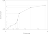 |
Fig. 1 Parameterisation of the problem. Extinction distance pairs are defined with respect to the previous pair. This line of sight extinction distribution requires 12 parameters. Linear interpolation was used to provide a continuous solution along the line of sight. |
3.2 Posterior probability
Using the MCMC method, we identified the line of sight extinction that provides the appropriate correction to the BGM so that the colour distributions of observed and modelled stars are in agreement. The criteria for this agreement is a Poisson likelihood applied to the J–H and H–KS colour histograms.
The Bayes theorem states that the posterior probability of the model parameters, θ, given the observations, Y, is
 (3)
where p(θ) describes the prior and P(Y) is the evidence. As we search for the best parameters given a set of observations, the denominator is simply a constant that we can neglect, as it has no dependence on the model parameters.
(3)
where p(θ) describes the prior and P(Y) is the evidence. As we search for the best parameters given a set of observations, the denominator is simply a constant that we can neglect, as it has no dependence on the model parameters.
The histogram bin contents are assumed to be individual Poisson distributions. Thus the likelihood of observing n stars given the model that predicts λ stars is
 (4)
(4)
This likelihood function models the probability of observing ni stars in each bin given the Poisson-distributed expectation λi predicted by the BGM. The log likelihood is easier to work with and is simply
 (5)
where we drop the factorial term that is independent of the model counts (λi). In the high count regime, the Poisson distribution asymptotically approaches a Gaussian distribution with mean λi and variance λi. The log-likelihood becomes quadratic in ni −λi and resembles least-squared minimisation.
(5)
where we drop the factorial term that is independent of the model counts (λi). In the high count regime, the Poisson distribution asymptotically approaches a Gaussian distribution with mean λi and variance λi. The log-likelihood becomes quadratic in ni −λi and resembles least-squared minimisation.
For the prior, we have chosen a simple implementation to ensure that our Markov chain does not explore solutions beyond the maximum distance and extinction that we derived above. Below these maxima we use a uniform prior but, to avoid a hard limit, we apply an exponential probability to values above the maxima. The scale parameters we use are approximately our sensitivity thresholds in distance and extinction, resulting in a value of 10 pc (BGM step size) and 0.03 mag in AK (uncertainty in 2MASS colours Marshall et al. 2006).
3.3 Metropolis–Hastings ratio
The parameter space was explored using a customised Metropolis-Hastings algorithm written in Fortran. For a given line of sight, we attempt to deduce the most probable line of sight extinction. We do not simply want to obtain the best estimate but also a measure of the uncertainty of this distribution.
We used the Metropolis–Hastings algorithm to directly sample this probability distribution in the distance-extinction plane (Fig. 1), π(x), where x is the parameter vector. We initialised the parameters as described in Sect. 3.1 and then explored the parameter space using a proposal function. If the current state of the chain is at x, then the proposal function will provide the next state via
 (6)
where we simply use ϕ(x), the standard normal density. The new state may be in a higher or lower probability region, and the Metropolis-Hastings ratio is used to determine whether the new state is accepted or not. The ratio is given by
(6)
where we simply use ϕ(x), the standard normal density. The new state may be in a higher or lower probability region, and the Metropolis-Hastings ratio is used to determine whether the new state is accepted or not. The ratio is given by
 (7)
(7)
This is often simplified to π(x∗)/π(x), as the standard normal density is symmetric. In our case a proposal that results in a negative value for a parameter must be rejected, as it would result in negative extinction. This was avoided by taking the absolute value of the proposal, thereby mapping the negative values onto positive ones. However, this is not an ideal situation for exploring the parameter space, as the proposal distribution is no longer symmetric. We address this point when presenting the analysis of the map (Sect. 4.1.4).
3.4 Spurious structure at large distances
As mentioned above, a maximum distance and extinction are enforced through the use of a simple exponential prior, but this prior is uniform below these maxima. Due to the way REDLINE is implemented, with a fixed number of distance-extinction bins for a given line of sight, it is possible that the Markov chain finds solutions at large distance that have low or negligible effect on the likelihood. This is because at these distances stars are few and far between – they are certainly too few to significantly constrain structure in the ISM.
Once a solution was found for a given line of sight, the most faraway distance-extinction bins were tested for significance. This was achieved by removing them, one by one, from the line of sight solution and comparing this new solution with the solution that includes them. To test the difference between these two solutions, which are in fact two different models with different numbers of parameters, we calculated the Bayesian information criteria (BIC) for each model:
 (8)
where k = 2 × Nbins is the number of parameters, n is the number of colour bins used in the histograms, and ℒ is the likelihood as defined above. The usual use of the BICLis to test whether the addition of more parameters to a model results in a significantly better fit and hence avoid the possibility of overfitting. Indeed, one would expect the likelihood to improve as one adds more parameters to a model, as there are more degrees of freedom with which to fit the data. When comparing two models, the model with the lowest BIC is preferred. According to Kass & Raftery (1995), a difference of ten or more is strong evidence for the lower BIC model. As we remove bins we require the BIC to increase by at least ten in order to retain the last bin. If it is retained then we stop there. If it is rejected we continue towards closer bins to test their significance.
(8)
where k = 2 × Nbins is the number of parameters, n is the number of colour bins used in the histograms, and ℒ is the likelihood as defined above. The usual use of the BICLis to test whether the addition of more parameters to a model results in a significantly better fit and hence avoid the possibility of overfitting. Indeed, one would expect the likelihood to improve as one adds more parameters to a model, as there are more degrees of freedom with which to fit the data. When comparing two models, the model with the lowest BIC is preferred. According to Kass & Raftery (1995), a difference of ten or more is strong evidence for the lower BIC model. As we remove bins we require the BIC to increase by at least ten in order to retain the last bin. If it is retained then we stop there. If it is rejected we continue towards closer bins to test their significance.
We regrid the line of sight extinction to a constant 100 pc distance grid. The voxels beyond the furthest distance bin were all assigned the maximum extinction found for that line of sight. As the extinction is constant after this point the final density map has many zero values – some of which are significant, while others are simply missing data. To prevent the spurious retention of these zero-extinction bins at large distances – where the scarcity of stars renders any inferred ‘zero’ extinction statistically meaningless – we introduced a maximum reporting distance, Dmax, based on the Poisson sampling of synthetic stars. Along each sightline, the number of model stars in a thin shell at distance d is assumed to follow a Poisson distribution with the following mean:
 where λ0 is the line of sight stellar density at d = 0 and h is the exponential scale length. The value of h is itself determined via maximum-likelihood estimation on the unbinned reddened model stars, ensuring an unbiased fit to the simulated star counts. We required that at d = Dmax, there remains at least a 3σ confidence (P ≥ 0.997) of observing Nmin = 10 real stars. For a Poisson random variable N ∼ Pois(λ), this condition reads as

Substituting λ = λ0 e−d/h transforms the requirement into the root-finding equation whose solution d = Dmax is obtained numerically. All extinction bins at distances d > Dmax are then masked (set to NaN), ensuring that the final map reports only those regions where stellar sampling is sufficiently robust to constrain the ISM structure.
Although this criterion was devised to eliminate misleading ‘zero-extinction’ tails, we find that in some lines of sight the posterior inference predicts significant extinction at d > Dmax. Such high-extinction tails likely arise from reddening a minute fraction of model stars in order to match a small number of observed, highly reddened outliers, and do not reflect genuine large-distance ISM structure. At any rate as there are few stars available to constrain these distant structures, these extinction bins were likewise set to NaN when they were beyond Dmax as defined above.
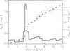 |
Fig. 2 Result of REDLINE in the presence of a single cloud using simulated observations. The diamonds with error bars are the different distance-extinction pairs (left axis), the solid line is the derivative of the extinction with respect to distance, the dashed line is the diffuse extinction, and the dotted lines show the 1 and 2-σ levels (right axis). Here a cloud is clearly detected at 4 kpc, identical to the injected cloud distance. |
3.5 Output for individual lines of sight
Figure 2 presents REDLINE’s performance using simulated data. We used the BGM to simulate a line of sight where stars experience a diffuse extinction of 0.7 mag/kpc in the V band, plus a cloud with AV = 5 mag at 4 kpc distance. The simulation included photometric errors based on magnitude, matching typical 2MASS catalogue observations along a single line of sight. In this figure the extinction is shown as a function of distance as well as the differential extinction per distance bin, providing a visualisation of the dust density along this line of sight. A mean baseline level of extinction was established off-cloud (dashed line), along with the 1 and 2-σ deviation around the mean (dotted line). REDLINE correctly identified both the simulated cloud at 4 kpc and captured the diffuse extinction component within the error bars.
The simulated line of sight given in Fig. 2 shows that the rise in extinction at the cloud distance is not necessarily completely vertical. This means that the extinction due to the cloud may be spread out along a finite distance interval. This is even more pronounced in real data, where cloud porosity and embedded stars make the distance determination less well defined than in the ideal simulated case. Furthermore, each distance-extinction pair is accompanied by its own respective uncertainties.
In Fig. 3, we show four lines of sight using real data that highlight different physical conditions. In each case, the extinction is shown as a number of points along the line of sight and a histogram showing the dust density (the derivative of the extinction as a function of distance). In three of the four lines of sight, one or more clouds rise above the 2-σ level of the background extinction. In the bottom left frame, the dust density at a distance of zero is above the 2-σ level, indicating that there were insufficient observed stars to detect the rise of extinction at low distance. In the final case, no clouds are detected.
This last case highlights an important limitation of these extinction methods. If no stars are detected due to high extinction, the associated dust will, of course, be absent from the map. This can also bias distance measurements to structures where some stars are beyond detection due to extinction. In these cases, only the lower density areas of a cloud will be detected, possibly at a different distance from the actual cloud centroid.
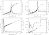 |
Fig. 3 Example lines of sight using real data in a 15′ by 15′ pixel towards prestellar cloud candidates (Planck Collaboration XXVIII 2016). Clockwise from the top left, the panels show one detected cloud (l = 9.25, b = −0.2), two detected clouds (l = 17.2, b = −1.5), no detections (l = 215, b = 4.1), and finally one detected cloud with only an upper limit for the distance (l = 159.7, b = −0.9). Symbols and line styles are as in Fig. 2. The fields shown here were chosen to sample different environments and are not all in the final footprint of the map presented in this paper. |
4 Results and discussion
REDLINE has been executed across the entire Galactic plane within the latitude range of |b| ≤ 1°. For each individual line of sight, the extinction was calculated independently utilising a pixel dimension of 10′ × 10′. To enhance the spatial resolution and better capture the structures present in the ISM, the sampling across the sky was conducted in incremental steps of 5′. This approach yields detailed maps on a 5′ grid while maintaining a consistent angular resolution of 10′.
4.1 Presentation of the map
4.1.1 Polar projection
The Galactic plane as seen from the North Galactic Pole is shown in Fig. 4 where the median value over |b| ≤ 1° is plotted. The Solar position is at the origin with the Galactic centre off to the right at x = 8.0, y = 0. The quantity plotted here is proportional to dust density, and is simply the derivative of visual extinction with respect to distance along each line of sight.
One obvious characteristic in this map is a spreading out of structures along the line of sight, creating features that seem to be pointing towards the Solar position. For a certain number of these structures, however, this elongation is to be expected as the corresponding lines of sight follow spiral arm tangencies, sometimes measuring several kpc, for example along l ≈ 315°. Along this particular direction, the line of sight follows the Crux spiral arm tangency for several kpc. As illustrated in Fig. 2, REDLINE can smear compact features over scales of about a kiloparsec, even for individual pre-stellar clouds. This effect also impacts more extended structures such as spiral arm tangencies, whose lengths are likely overestimated in the REDLINE map. Another aspect of the map is the difference between the inner Galaxy and the anticentre direction. Many lines of sight in the outer Galaxy end with little to no extinction. They are limited by the number of stars observable at these large Galactocentric radii. In the inner Galaxy, however, line of sight end with significant extinction, showing that it is the high extinction here that limits the distance range of the REDLINE map.
To enhance the visibility of structural features in our Galactic map, we employed a differential smoothing technique. This method involves subtracting two Gaussian-smoothed versions of the map: one with a relatively fine smoothing scale of 100 pc, and another with a broader 1 kpc smoothing kernel. This approach, analogous to unsharp masking, effectively isolates intermediate-scale structures while removing larger-scale background variations. The resulting difference map emphasises overdensities at scales between these two smoothing lengths, making it particularly effective for identifying and analysing Galactic structural features that might otherwise be difficult to discern in the original data. The resulting map is shown in Fig. 5, where the overlaid spiral arms are a result of a fit described below (Sect. 4.2).
In this image, one can spot the fiducial spiral arm tangencies of Sagittarius (l ∼ 50°), Scutum (l ∼ 30°), Norma (l ∼ 330°), Crux (l ∼ 315°), and Carina (l ∼ 285°). The local arm is seen towards Cygnus (l ∼ 80°) and Vela (l ∼ 280°).
The dust lanes of the Galactic bar are visible between l ± 10° but not much is detected beyond. This structure was more fully explored in Marshall et al. (2008). A lack of dust is seen in the inner ∼3 kpc around the Galactic centre.
The outer Galaxy is conspicuous for its overall lack of dust, and the relatively small distances to which REDLINE is able to probe in these directions. However, the overdensity map is particularly well suited to highlighting structure in this region. Indeed, some dust is clearly visible in this map, revealing a notable overdensity in the anti-centre region. This concentration of interstellar material appears to be associated with the Perseus spiral arm, one of the major structural features in this part of our galaxy’s disc.
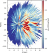 |
Fig. 4 REDLINE view of the Galactic plane as seen from the North Galactic Pole. The Sun is at the origin and the Galactic centre is at (x, y) = (8, 0). Dotted circles are plotted every 2 kpc around the solar position, and dashed lines are plotted every 30 degrees. The quantity plotted here is extinction per unit distance, and is proportional to dust density. There is a paucity of dust in the outer Galaxy, and most of the dust is seen to lie in the so-called molecular ring. |
4.1.2 Average extinction in the disc
REDLINE not only detects the dense structures comprising the molecular clouds associated with spiral arms and spurs but is also sensitive to extinction in the more diffuse ISM. To quantify the distribution of the diffuse dust component of the Galaxy, we calculated the median extinction in galactocentric distance bins. The distance bins were separated by 0.5 kpc, and the median was calculated for all extinction values between a Galactic azimuth of ±115°, where 0° is the Sun–Galactic centre direction. The result is the blue profile in the top panel of Fig. 6, where the error bars represent the mean absolute deviation in each distance bin.
This profile was then smoothed with a Gaussian filter with σ = 0.2 kpc (shown in orange). Assuming axisymmetry, the diffuse disc of the Galaxy can be obtained by rotating the smooth profile through 360° (Fig. 6, middle). In this representation, it can be seen that the diffuse extinction in the solar neighbourhood is approximately 0.7 mag/kpc, reaches ∼1.6 mag/kpc in the inner Galaxy, and drops off quickly in the outer Galaxy.
The radial profile at the top of Fig. 6 shows an exponential decrease beyond approximately 4 kpc. An exponential fit to the curve beyond 4.5 kpc is shown as a green dashed line, which was used to estimate the scale length of the Galactic dust disc. We found that the scale length is 3.4 ± 0.6 kpc. Inward of this position, there is a lack of dust as the Galactic bar sweeps up the central dust in its dustlanes (Marshall et al. 2008).
At the bottom of Fig. 6 we compare our results with those of the H2 surface density as derived from CO data (Heyer & Dame 2015, and references therein). Our data is plotted against the left vertical axis whereas the other data points use the right. An exact conversion in units is complicated by the fact that the dust traces all gas phases, assuming a constant dust-to-gas ratio, and not simply the molecular phase. The same exponentially decreasing trend is observed, however, and performing the same fit as above to the data from Bronfman et al. (1988) and Nakanishi & Sofue (2006) resulted in a molecular scale length of 2.8 ± 0.4 kpc and 2.8 ± 0.5 kpc, respectively.
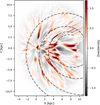 |
Fig. 5 Local dust overdensities relative to surrounding matter in the REDLINE map. To highlight regions where dust density significantly deviates from the ambient material, the map of the Galactic plane was first lightly smoothed and then a heavily smoothed version was subtracted from it. This technique enhances local density variations, effectively isolating overdense features from the broader background. The overlaid spiral arms are the result of a fit to the data and are explained in Sect. 4.2.2. |
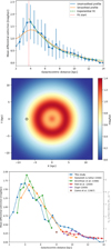 |
Fig. 6 Top: median interstellar extinction as a function of Galactic radius (blue line) as well as a smoothed version (orange line). Middle: average extinction in the Galactic plane. The solar position is indicated at x = −8, y = 0. Bottom: comparison of our dust density with the H2 mass surface density as a function of Galactic radius from Fig. 7 of Heyer & Dame (2015). Distances have been scaled to R⊙ = 8 kpc and the vertical axes have been arbitrarily scaled. |
4.1.3 Cartesian projection
The top-down view of the Galactic plane is often the first visualisation presented in this type of 3D study. It provides an interesting perspective as it gives us an idea of what our galaxy might look like to an outside observer. However, the intrinsic nature of the observations means that along a given line of sight, one samples a larger volume of space at greater distances. Thus, as we get closer to the Sun, these lines of sight become so narrow that it is difficult to trace the structure being detected by REDLINE.
To better visualise the data in terms of Galactic structure, we plotted the longitude-distance information in a Cartesian plot instead of polar coordinates. In Fig. 7, the full Galactic plane is once again shown in terms of dust density but in a Cartesian projection of longitude and distance.
In this projection, the different arms are more easily distinguished. In the crowded molecular ring region (∼50° < l < ∼−50°, 2 < d < 6 kpc), several structures can be identified. Although the four main ‘spiral arms’ account for the majority of the structure seen in the map, many features do not align with them. In the next subsection we perform logarithmic spiral fitting to the structures associated with the main arms.
4.1.4 Possible bias due to asymmetrical proposal distribution
As mentioned in Sect. 3.3, REDLINE’s distance extinction model parameters are defined as increments relative to preceding parameters. These increments cannot be negative by design. When the MCMC proposal generates a negative increment, REDLINE takes its absolute value to maintain this constraint. However, this approach creates an asymmetry in the proposal distribution, violating the reversibility criterion essential for Markov chains. This violation could potentially affect the chain’s ability to efficiently explore the parameter space.
To identify regions where this violation might impact our results, we analysed each line of sight by examining the separation between neighbouring bins in both extinction and distance. We specifically looked for cases where these separations were smaller than or equal to the standard deviation of the Gaussian proposal distribution used in the MCMC. Such cases would indicate areas where the reversibility criterion violation could affect the results. Our analysis revealed that fewer than 1% of the lines of sight in the final map met these criteria, suggesting minimal impact on our overall results. Nevertheless, we plan to address this limitation in a future version of REDLINE.
4.2 Spiral arm structure
The Milky Way’s spiral arms are prominent features of our galaxy’s structure, characterised by enhanced densities of stars, gas, and dust. These arms can be traced through various observational methods, with dust being a particularly useful tracer due to its close association with star formation regions. Matter that follows a logarithmic spiral with pitch angle p will have its maximum intensity at a galactocentric distance r that depends on the Galactic azimuthal angle θ:
 (9)
where θ is taken to increase counterclockwise from the Sun– Galactic centre axis and k = tan(p), r0, and θ0 are constants that scale or rotate the spiral arm about the Galactic centre, respectively. These two constants are in fact degenerate, as a change in one can be counterbalanced by a change in the other. Often the spiral arms are taken to be symmetric so that r0 is constant for all four arms, but they are rotated with respect to each other by incrementing θ0 by π/2 between adjacent arms.
(9)
where θ is taken to increase counterclockwise from the Sun– Galactic centre axis and k = tan(p), r0, and θ0 are constants that scale or rotate the spiral arm about the Galactic centre, respectively. These two constants are in fact degenerate, as a change in one can be counterbalanced by a change in the other. Often the spiral arms are taken to be symmetric so that r0 is constant for all four arms, but they are rotated with respect to each other by incrementing θ0 by π/2 between adjacent arms.
In the following, we constrain the parameters of the main spiral arms of the Milky Way using the REDLINE map. However, we took θ0 = 0 for all arms and tried to deduce r0 and pitch angle p independently for each arm.
Where two tangents to the spiral arm can be identified on either side of the Sun–Galactic centre line, the twin tangent method (Vallée 2015) can be used to derive the pitch angle. In cases where two tangents cannot be identified, one can look at the Galactic structures in the Galactic azimuth-log Galactic distance plane. In this projection, spiral structures appear as straight lines. It is then possible to find the best-fit linear model to obtain the r0 and pitch angle simultaneously. This also provides a check to the twin tangent method that does not take into account the intermediate matter between the two tangent points.
Finally, it can also be instructive to look at spiral structure in the longitude-distance plane directly, by first selecting the structure of interest in the REDLINE map. It is then possible to follow the structure around the Galactic centre using a density-weighted mean in the Galactic radial direction. To obtain a global picture of the main spiral structure in the Milky Way, we applied these three techniques in combination.
 |
Fig. 7 REDLINE results for the entire Galactic plane. The dust density is represented in a 2D longitude–distance plane. Note that this representation stretches structures out horizontally at low distance. (For a polar projection that does not do this see Fig. 4.) |
4.2.1 Twin tangent method
For three spiral arms, Norma, Scutum-Crux, and Sagittarius-Carina, two tangent points are observable, as they occur inside the solar circle. In the case of a ring shape around the Galactic centre, corresponding to a pitch angle of zero, one would expect the tangent points in the first and fourth quadrants to be symmetrical. As the pitch angle increases, so does the asymmetry of the location of the two tangent points. As such, the identification of the two tangent points provides a direct way to determine the pitch angle of a single spiral structure passing through both of them.
To determine the pitch angle of the spiral arms, we started by identifying structures associated with these tangent points before calculating a density-weighted mean to pinpoint the REDLINE view of them. In the next step, we followed Vallée (2015) and used the two tangent points to calculate the pitch angle, p, via
![Mathematical equation: $p = \arctan \left\{ {{{\ln \left[ {\sin \left( {{l_1}} \right)/\sin \left( {2\pi - {l_4}} \right)} \right]} \over {{l_1} - {l_4} + \pi }}} \right\},$](/articles/aa/full_html/2025/12/aa54622-25/aa54622-25-eq12.png) (10)
where l1 and l4 denote the longitude of the tangent points of the spiral arm in the first and fourth Galactic quadrants, respectively.
(10)
where l1 and l4 denote the longitude of the tangent points of the spiral arm in the first and fourth Galactic quadrants, respectively.
The twin tangent method is only useful if we are able to accurately pinpoint the location of the tangencies. Different observational markers of the tangencies have been reported (Vallée 2014, 2015) and can vary depending on the tracer.
In order to identify the spiral arm tangencies in the RED-LINE map, we needed to identify a search region for each one. The tangencies should show up as an elongated structure in a longitude range compatible with the tangencies identified in the literature. We inspected the REDLINE map near the literature values to define the search area. The distance range was chosen by eye to include the structure. The chosen zones for the search are summarised in Table 2.
In each search zone, we extracted the REDLINE data and created a 2D skymap and mean longitude profile (Figs. A.1, A.2 and A.3). We neglected extinction associated with the diffuse phase at the galactrocentric distance of the tangent (cf. Fig. 6). We then performed a weighted mean and standard deviation to obtain the location of the tangent and associated uncertainty. The resulting values are shown in Table 2.
Using the locations of these tangent points, a first estimate of the pitch angles of the spiral arms was determined. We found a pitch of 7.2 ± 1.2° for Norma, 12.2 ± 1.7° for Scutum-Crux and 13.8 ± 1.2° for Sagittarius-Carina.
Tangencies of the spiral arms as determined from the extinction map.
4.2.2 Fitting spiral parameters with multiple constraints
In this section, we focus on utilising the REDLINE map to derive the large-scale spiral structure of the Milky Way. It is important to note that our analysis remains within the scope of the traditionally defined spiral arms, as originally identified in longitude-velocity space, where the identification of tangencies played a crucial role in shaping the model of these arms. Future research may involve fitting more complex models that incorporate varying pitch angles and the identification of spurs, among other features.
In order to constrain the pitch angle of the spiral arms using both the location of the tangents as well as the dust density between the tangents, we proceeded as follows. For each spiral arm with two tangencies (Norma, Scutum-Crux and Sagittarius-Carina), we employed two likelihood terms. The first is based on the dust density distribution across the arm, while the second uses tangencies identified in our REDLINE map. To identify these tangencies, as mentioned above, we defined search windows based on established tangency positions from the literature. While this approach means our analysis was influenced by existing models of Galactic structure, it provides a framework to examine how the REDLINE map aligns with the current understanding of spiral structure. The search windows helped focus our analysis on relevant regions while still allowing the exact tangency positions to be determined by the dust distribution in our map.
We varied the two parameters in our spiral arm model, namely the radial normalisation r0 and the pitch angle p (while fixing θ0 = 0, as discussed above) using a brute force search. The variation was performed with a regular step size of 0.01 in r0 and 0.1 in p. For each (r0, p) pair we evaluated both likelihoods. For the Perseus arm, which has no tangencies as viewed from the solar position, we used only the dust density likelihood.
For the first of these two terms, we compared the position of the model arm with respect to the weighted distance and associated standard deviation of the dust in the REDLINE map, using dust density as weights. We assumed that dust density across a spiral arm follows a Gaussian distribution. This enabled us to calculate a likelihood of the model parameters given the data for a given line of sight:
 (11)
where r is the (galactocentric) distance to the model arm derived using r0 and p via Eq. (9), and µ and σ are the weighted mean and standard deviation of the distance to the dust of the arm in the REDLINE map. This likelihood was calculated across the azimuthal range where the arm appears, in bins of 2.5°. Taking the log of this likelihood and dropping any constant terms gives
(11)
where r is the (galactocentric) distance to the model arm derived using r0 and p via Eq. (9), and µ and σ are the weighted mean and standard deviation of the distance to the dust of the arm in the REDLINE map. This likelihood was calculated across the azimuthal range where the arm appears, in bins of 2.5°. Taking the log of this likelihood and dropping any constant terms gives
![Mathematical equation: $\ln \left( {{{\cal L}_{{\rm{arm}}}}} \right) = - \mathop \sum \limits_{i = 1}^N \left[ {\ln \left( {{\sigma _i}} \right) + {{{{\left( {{r_i} - {\mu _i}} \right)}^2}} \over {2\sigma _i^2}}} \right].$](/articles/aa/full_html/2025/12/aa54622-25/aa54622-25-eq14.png) (12)
(12)
Here, N is the number of azimuthal bins, and the i subscript denotes the values of r, µ, and σ for the ith bin.
We also used the tangencies of the model arm to calculate a likelihood by comparing them to the means ℓ1 and ℓ4 (in the first and fourth quadrants, respectively) and standard deviations σ1 and σ4 of the tangencies as determined using the REDLINE map. The log-likelihood of the model tangencies given the ones found in the REDLINE map is
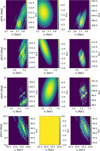 |
Fig. 8 Log likelihood of spiral parameters for the four major arms. From the top row to the bottom row, the panels show Norma, Scutum-Crux, Sagittarius-Carina, and Perseus, respectively. The left column shows the density likelihood, the middle column is the tangent likelihood, and the right column is the combination of both. Note that Perseus has no tangents, so the likelihood is flat. |
 (13)
where
(13)
where  and
and  are the locations of the tangencies for the model in the first and fourth quadrants, respectively. The total log-likelihood is the sum of the individual log likelihoods.
The results for each likelihood and the combined one for each arm are presented in Fig. 8. We used the resulting 2D log-likelihood distribution to obtain estimates for r0 and p along with uncertainties for each arm by fitting a 2D Gaussian to the distribution. The resulting parameters for the four classic spiral arms of the Milky Way are shown in Table 3, alongside those from Reid et al. (2019). They are also plotted in Fig. 5.
Figure 9 presents a detailed view of our galaxy’s spiral arms near their tangent points. Through a series of paired plots, we show both the spatial distribution and longitudinal relationships of masers associated with the major spiral arms as seen in the REDLINE map. We also plot the derived spiral arms on the longitude-distance representation of the REDLINE map in Fig. 10.
A key observation from the REDLINE map is that dust is distributed throughout the Galactic disc in a highly non-uniform manner. While the classical spiral arm loci do contain enhanced concentrations of matter, there is no evidence for continuous spiral arms. Instead, we observe a fragmented structure where clumps of matter align approximately along the expected spiral patterns, interspersed with regions of significantly reduced density where spiral arms ‘should be’ according to idealised logarithmic models. Furthermore, there is significant structure between the spiral arms of the model.
This fragmented nature is particularly evident when examining specific arms. Referring to either Fig. 9 or Fig. 10, matter does indeed appear to follow the Scutum-Crux arm relatively well, though with notable gaps and overdensities rather than a smooth distribution. For the Sagittarius-Carina arm, while the tangents are well represented, between 50°≥ l ≥ 30° the dust in the REDLINE map associated with the Sagittarius arm deviates substantially from the perfect logarithmic prediction, as reported in the free electron distribution by Taylor & Cordes (1993). Further there is a distinct lack of matter on the spiral loci of the Sagittarius-Carina arm between −45° < l < −70°. The Perseus arm shows even less coherent matter distribution along its predicted path (Fig. 9).
Figure 11 compares our spiral arm analysis with the previous work of Reid et al. (2019), whose spiral arm parameters are displayed in Table 3. The REDLINE overdensity map provides the background to both models and to the maser positions. The two models show remarkable agreement in their overall structure, especially considering that the underlying data are completely independent. There are some differences in the detailed arm trajectories, which can be partly attributed to different modelling approaches, as Reid et al. (2019) employed a more complex model allowing for two pitch angles within individual arms, introducing two additional degrees of freedom compared to our approach.
A significant shift exists between our position of the Norma arm in the first quadrant and the position of the masers associated with this arm segment. Another notable deviation between the two models occurs in the far Sagittarius arm in the first quadrant, beyond the tangent point at ℓ = 50°. In this region of the Galaxy, the structures in the REDLINE map are more spread out, and the maser positions also show considerable scatter, making precise mapping of spiral structure challenging.
Parameters of the classic spiral arms in the Milky Way as derived from the REDLINE map and compared with the fit from R19.
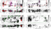 |
Fig. 9 Spiral arm structure near tangent points. The figure is arranged in four quadrants with each containing paired images showing longitude-distance relationships (top) and corresponding sky distributions (bottom). Top left: Scutum and Norma arms (first quadrant). Top right: Crux and Norma arms (fourth quadrant). Bottom left: Sagittarius arm. Bottom right: Carina arm. Spiral arm fits (Sect. 4.2.2) are shown as dotted lines, with maser positions and their error bars colour-coded by arm: Norma (magenta), Scutum/Crux (red), and Sagittarius/Carina (green) |
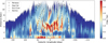 |
Fig. 10 Same as Fig. 7 but with the results of the spiral arm fitting. Much of the structure of the map can be attributed to this spiral structure; however, there are also a number of exceptions, most notably the dust lanes associated with the Galactic bar. |
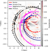 |
Fig. 11 REDLINE overdensity map in greyscale with spiral arm fits from this study (dashed lines) and from Reid et al. (2019) (solid lines) overlaid. Masers from Reid et al. (2019) are also plotted for comparison. In all datasets, colours indicate the corresponding spiral arm or its association, as detailed in the legend. |
4.2.3 Comparison with observed stellar structures
Recently, Gaia Collaboration (2023a) examined the spiral structure within 4 kpc of the Sun by selecting and mapping OB stars in the Galactic plane with a kernel-based density estimator. They observed that these young and massive stars cluster into distinct high-density regions corresponding to well-known spiral arms – namely, the Perseus arm, the Local (Orion) Arm, and parts of the Sagittarius-Carina/Scutum arms. Within roughly 3 kpc of the Sun, these structures are quite pronounced, but beyond this range, foreground extinction increasingly creates radial “shadow” cones that obscure the stellar distribution.
Their analysis also includes a map of local overdensities in the OB stellar population (Fig. 12, left). Notably, they find that the Local Arm extends for about 8 kpc, indicating that it is neither a minor arm nor merely a spur. Although the authors do not provide a pitch angle for this arm, their map suggests a significantly more open structure than that seen in our study.
A direct comparison between their stellar overdensity map (Fig. 12, left) and the REDLINE dust map (Fig. 12, middle) highlights that many apparent stellar features may be traced back to line-of-sight extinction – even within the 3 kpc limit. In numerous regions, these two maps resemble near-inverses of each other (Fig. 12, right). Specifically, areas with high stellar density often show a corresponding deficit of dust – such as near x = 2 kpc, y = 0.5 kpc – whereas zones devoid of stars coincide with substantial dust concentrations (for example, near x = 0.5, y = 2).
Looking ahead, a combined analysis that accounts for both stellar overdensities and the dust distribution will offer a more robust picture of the Milky Way’s spiral structure than methods focusing solely on one or the other.
4.3 The Galactic bar
Another Galactic structure that stands out in the REDLINE map is the dust surrounding the Galactic bar. These dust lanes precede the stellar bar as it rotates, sweeping up dust and gas. Marshall et al. (2008) studied the dust extinction of this Galactic feature and compared it to the CO emission via the Galactic kinematic model of Fux (1999). The dust lanes were found to be tilted with respect to the b = 0° plane in both dust and molecular gas. Here we isolated the dust lanes using similar cuts to see if the same results hold with REDLINE.
In Fig. 13, the REDLINE map around the Galactic centre is displayed. At the top of this figure the top down view is shown, where the extinction due to the dust lanes can be seen clearly. There are areas of this map where no valid extinction values have been obtained by REDLINE, shown as white in this map. Two dotted lines highlight the area that was chosen, by eye, to contain the dust lanes. Note that the orientation of these dust lanes is not the same as that of the stellar bar, which in the version of the BGM used has an angle of α = 12.8° with respect to the Sun– Galactic centre line. Indeed, the dust can be seen to lie ahead of the bar as it rotates about the Galactic centre, with the dust lying behind the stellar bar at positive longitudes and in front of the bar at negative longitudes.
On the bottom of Fig. 13 the extinction within the chosen zone of the top image is integrated along the line of sight, and then subject to a Gaussian filter to bring the resolution into agreement with the CO data as was done in Marshall et al. (2008). The same trend is seen here as was reported by Marshall et al. (2008), namely that the midplane of the dust lanes are tilted with respect to the b = 0° plane, with the negative longitude part lying above the plane and the positive longitude part lying below the plane. It is likely that this sky plane image is an underestimate as there are many areas with missing data, especially at the negative longitudes.
The structures revealed in our extinction map show notable correspondences with features identified in the molecular gas analysis of Sormani et al. (2019). In particular, we find evidence for both the L1 and L4 structures (see their Figure 1). The L1 feature appears near b ≈ −0.8° between l = 8° and l = 4°. From there, it rises to nearly b = 0° between l = 4° and l = 3.2°, and remains at this latitude up to l = 2°. The L4 structure is traced starting close to b = 0° between l = −1° and l = −3.2°, then it rises to nearly b = 1° at l = −4°. We also detect extinction associated with the region of the extreme-velocity cloud at l = 3.2°. By contrast, our map does not show evidence for the L2 feature, which should appear at positive longitudes near b = 0.8°. The L3 structure may be present but appears superimposed on L1 between l = 4° and l = 2°, making it difficult to disentangle even in the top-down view. Finally, neither the central molecular zone (likely too dense to be traced by REDLINE) nor the extreme-velocity cloud at l = 5.4° are detected in our extinction map.
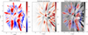 |
Fig. 12 Left: reproduction of the Gaia Collaboration (2023a) OB stellar overdensity map. Centre: dust overdensity (this work) shown with the same Galactic coordinate system for direct comparison. Right: greyscale dust overdensity overlaid with coloured contours of OB stellar overdensity. The red contours highlight regions where stellar features coincide with low-dust zones (white in the background), while the blue contours trace apparent stellar ‘gaps’ that align with high-dust concentrations (dark grey to black in the background). |
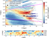 |
Fig. 13 Top: top-down view of the Galactic centre region. The Galactic centre is marked with a star, and the stellar bar, as modelled by the BGM, is indicated by the dashed line. The dotted lines delimit the region selected for the study of the dust lanes. Bottom: sky projection of the dust distribution within the region defined by the dotted lines in the top panel. The longitude range used is indicated by the magenta dashed line in the top panel. The dust lanes exhibit a clear tilt: at negative longitudes, the dust lies above the Galactic plane (b = 0°), while at positive longitudes, it lies below. |
4.4 Comparison with Zucker et al. (2025)
Zucker et al. (2025) have very recently created a high-resolution 3D map of interstellar dust across a significant portion of the southern Galactic plane (−120° < l < 6° and |b| < 10°). They use photometric data from four major surveys – DECaPS2, VVV, 2MASS, and unWISE – to calculate key stellar parameters for approximately one billion stars. Parallax data from Gaia are used when available. They combine their results with those from Bayestar (Green et al. 2019) to cover the entire Galactic plane.
In Fig. 14, we compare our 3D dust map with theirs. While both maps provide a comprehensive view of the Galactic dust distribution, our approach offers a distinct perspective by relying solely on near-infrared stellar observations, enabling us to achieve a higher sensitivity at large distances (and thus through higher extinctions). Zucker et al. (2025), on the other hand, employs a star-by-star analysis to derive extinction and distance estimates, using data from the visible to the near-infrared, resulting in a highly detailed reconstruction at closer distances (d < 4 kpc).
Despite these methodological differences, both maps exhibit agreement in the large-scale distribution of dust, particularly in key structures within the third and fourth Galactic quadrants. Certain structures are identifiable in both maps but at different distances where our map tends to place structures further away from the Sun. Our map’s extended reach allows us to trace dust features convincingly beyond d ≳ 5 kpc, offering an unprecedented view of the Milky Way’s disc where Zucker et al. (2025) has limited sensitivity. Nevertheless, it is possible to identify structure at large distances in both maps, for example a structure we identify with the Carina arm at (x, y) ∼ (3, − 8).
At closer distances, the higher spatial resolution of Zucker et al. (2025) reveals finer details in the dust distribution, making it an excellent complement to our broader-scale method. A key advantage of our approach lies in its ability to provide a seamless and extended view of the Galactic plane, making it particularly suited for studies of large-scale Galactic structure. While Zucker et al. (2025) offers compelling insights into more nearby dust clouds, our results provide a complementary and far-reaching view, particularly in the inner Galaxy where the spiral structure remains challenging to map.
Future investigations will benefit from a detailed comparative analysis of both mapping approaches. By examining the discrepancies between the Zucker et al. (2025) map and our REDLINE map, we can better understand the limitations and strengths of each method. Understanding where and why these maps differ will help identify systematic biases and improve both approaches, ultimately leading to a more robust understanding of three-dimensional dust distribution across the Milky Way.
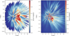 |
Fig. 14 REDLINE (left) and Bayestar (Green et al. 2019) + DECaPS 3D Dust (Zucker et al. 2025) (right) on the same physical and colour scale. The Sun is at the origin, and the Galactic concentric rings are plotted every 2 kpc and radial lines every 30 degrees. |
5 Conclusions
The REDLINE method represents a new way to map the three-dimensional structure of the ISM within the Milky Way. We used an MCMC approach to determine the 3D extinction distribution that corrects the Besançon model to be in agreement with 2MASS near-infrared stellar observations. The metric used to measure the similarity between observations and the model is the Poisson likelihood of the distribution in near-infrared stellar colours.
The method was applied to the full Galactic plane at |b| ≤ 1°. The resulting map provides predictions of ISM structure up to a distance of 15 kpc with a spatial binning of 100 pc, offering detailed insights into the distribution of dust and extinction in our galaxy. This map also enables a new level of exploration into the morphology of the inner Milky Way.
Our approach relies solely on near-infrared stellar observations, which allows for enhanced sensitivity through high-extinction regions, where traditional mapping techniques face limitations, particularly beyond 4 kpc from the Sun. The incorporation of an enhanced BGM provides more accurate stellar population predictions, further improving the reliability of our results. The final map features a 10′angular resolution on a 5′ grid with 100 pc binning in distance.
The map provides evidence for the large-scale spiral structures within the Galactic plane. Features corresponding to the known spiral arms and the Galactic bar are clearly identified. These results underscore the robustness of the REDLINE method as a tool for reconstructing Galactic morphology on large scales while also highlighting details previously unresolved in other studies.
However, the map also challenges traditional conceptions of the spiral arms as being continuous well-defined features. Instead, the arms appear fragmented, with significant gaps and discontinuities. These findings suggest that the Milky Way’s spiral structure may be more complex and dynamic than simpler models suggest, with the ISM distributed in a way that cannot be categorised into neat, uninterrupted arms. This fragmentation may result from ongoing star formation, feedback processes, and gravitational interactions that continuously shape and reshape the spiral structure.
In addition to the spiral arms, the REDLINE map reveals material in the inter-arm regions, with numerous spurs, branches, and other structures that do not fit into the classic four-arm model of the Milky Way. These features highlight the complexity of the ISM and suggest that significant structure exists even in regions separated from the loci of the major Galactic spiral arms.
Acknowledgements
We are grateful to Annie Robin for providing access to the BGM. DM would like to thank Bob Benjamin and Catherine Zucker for useful discussions. We are grateful to Eloisa Poggio for providing the data and code for the OB stellar overdensity map in Fig. 12 and Catherine Zucker for sharing her dust map for comparison in Fig. 14. This research was supported by the Programme National “Physique et Chimie du Milieu Interstellaire” (PCMI) of CNRS/INSU with INC/INP co-funded by CEA and CNES. This research has been partially supported by the EU-funded VIALACTEA Network (Ref. FP7-SPACE-607380). This publication makes use of data products from the Two Micron All Sky Survey, which is a joint project of the University of Massachusetts and the Infrared Processing and Analysis Center/California Institute of Technology, funded by the National Aeronautics and Space Administration and the National Science Foundation. The CDSClient package was used for the remote querying of the 2MASS dataset.
References
- Amôres, E. B., Robin, A. C., & Reylé, C. 2017, A&A, 602, A67 [NASA ADS] [CrossRef] [EDP Sciences] [Google Scholar]
- Arenou, F., Grenon, M., & Gomez, A. 1992, A&A, 258, 104 [NASA ADS] [Google Scholar]
- Aumer, M., & Binney, J. J. 2009, MNRAS, 397, 1286 [NASA ADS] [CrossRef] [Google Scholar]
- Baraffe, I., Chabrier, G., Allard, F., & Hauschildt, P. H. 1997, A&A, 327, 1054 [Google Scholar]
- Bertelli, G., Nasi, E., Girardi, L., & Marigo, P. 2009, A&A, 508, 355 [NASA ADS] [CrossRef] [EDP Sciences] [Google Scholar]
- Bronfman, L., Cohen, R. S., Alvarez, H., May, J., & Thaddeus, P. 1988, ApJ, 324, 248 [NASA ADS] [CrossRef] [Google Scholar]
- Brunthaler, A., Reid, M. J., Menten, K. M., et al. 2011, Astron. Nachr., 332, 461 [Google Scholar]
- Burton, W. B. 1971, A&A, 10, 76 [NASA ADS] [Google Scholar]
- Chambers, K. C., Magnier, E. A., Metcalfe, N., et al. 2016, arXiv e-prints [arXiv:1612.05560] [Google Scholar]
- Churchwell, E., Babler, B. L., Meade, M. R., et al. 2009, PASP, 121, 213 [Google Scholar]
- Czekaj, M. A., Robin, A. C., Figueras, F., Luri, X., & Haywood, M. 2014, A&A, 564, A102 [NASA ADS] [CrossRef] [EDP Sciences] [Google Scholar]
- Edenhofer, G., Zucker, C., Frank, P., et al. 2024, A&A, 685, A82 [NASA ADS] [CrossRef] [EDP Sciences] [Google Scholar]
- Fux, R. 1999, A&A, 345, 787 [NASA ADS] [Google Scholar]
- Gaia Collaboration (Drimmel, R., et al.) 2023a, A&A, 674, A37 [CrossRef] [EDP Sciences] [Google Scholar]
- Gaia Collaboration (Vallenari, A., et al.) 2023b, A&A, 674, A1 [NASA ADS] [CrossRef] [EDP Sciences] [Google Scholar]
- Green, G. M., Schlafly, E., Zucker, C., Speagle, J. S., & Finkbeiner, D. 2019, ApJ, 887, 93 [NASA ADS] [CrossRef] [Google Scholar]
- Heyer, M., & Dame, T. M. 2015, A&A, 53, 583 [Google Scholar]
- Kass, R. E., & Raftery, A. E. 1995, J. Am. Statist. Assoc., 90, 773 [CrossRef] [Google Scholar]
- Lagarde, N., Decressin, T., Charbonnel, C., et al. 2012, A&A, 543, A108 [NASA ADS] [CrossRef] [EDP Sciences] [Google Scholar]
- Leike, R. H., Glatzle, M., & Enßlin, T. A. 2020, A&A, 639, A138 [NASA ADS] [CrossRef] [EDP Sciences] [Google Scholar]
- Marshall, D. J., Robin, A. C., Reylé, C., Schultheis, M., & Picaud, S. 2006, A&A, 453, 635 [NASA ADS] [CrossRef] [EDP Sciences] [Google Scholar]
- Marshall, D. J., Fux, R., Robin, A. C., & Reylé, C. 2008, A&A, 477, L21 [NASA ADS] [CrossRef] [EDP Sciences] [Google Scholar]
- Marshall, D. J., Joncas, G., & Jones, A. P. 2009, ApJ, 706, 727 [Google Scholar]
- Minniti, D., Lucas, P. W., Emerson, J. P., et al. 2010, New Astron., 15, 433 [Google Scholar]
- Nakanishi, H., & Sofue, Y. 2006, PASJ, 58, 847 [NASA ADS] [Google Scholar]
- Neckel, Th., & Klare, G. 1980, A&A, 42, 251 [Google Scholar]
- Peek, J. E. G., Tchernyshyov, K., & Miville-Deschenes, M.-A. 2022, ApJ, 925, 201 [NASA ADS] [CrossRef] [Google Scholar]
- Planck Collaboration XXVIII. 2016, A&A, 594, A28 [NASA ADS] [CrossRef] [EDP Sciences] [Google Scholar]
- Reid, M. J., Menten, K. M., Brunthaler, A., et al. 2014, ApJ, 783, 130 [Google Scholar]
- Reid, M. J., Menten, K. M., Brunthaler, A., et al. 2019, ApJ, 885, 131 [Google Scholar]
- Robin, A. C., Reylé, C., Derrière, S., & Picaud, S. 2003, A&A, 409, 523 [NASA ADS] [CrossRef] [EDP Sciences] [Google Scholar]
- Robin, A. C., Marshall, D. J., Schultheis, M., & Reylé, C. 2012, A&A, 538, A106 [NASA ADS] [CrossRef] [EDP Sciences] [Google Scholar]
- Saydjari, A. K., Schlafly, E. F., Lang, D., et al. 2023, ApJS, 264, 28 [NASA ADS] [CrossRef] [Google Scholar]
- Schlafly, E. F., Meisner, A. M., & Green, G. M. 2019, ApJS, 240, 30 [Google Scholar]
- Skrutskie, M. F., Cutri, R. M., Stiening, R., et al. 2006, AJ, 131, 1163 [NASA ADS] [CrossRef] [Google Scholar]
- Sormani, M. C., Treß, R. G., Glover, S. C. O., et al. 2019, MNRAS, 488, 4663 [NASA ADS] [CrossRef] [Google Scholar]
- Taylor, J. H., & Cordes, J. M. 1993, ApJ, 411, 674 [Google Scholar]
- Vallée, J. P. 2014, AJ, 148, 5 [Google Scholar]
- Vallée, J. P. 2015, MNRAS, 450, 4277 [Google Scholar]
- VERA Collaboration (Hirota, T., et al.) 2020, PASJ, 72, 50 [Google Scholar]
- Vergely, J. L., Lallement, R., & Cox, N. L. J. 2022, A&A, 664, A174 [NASA ADS] [CrossRef] [EDP Sciences] [Google Scholar]
- Xu, Y., Reid, M., Dame, T., et al. 2016, Sci. Adv., 2, e1600878 [NASA ADS] [CrossRef] [Google Scholar]
- Zucker, C., Saydjari, A. K., Speagle, J. S., et al. 2025, ApJ, 992, 39 [Google Scholar]
Chosen to be well beyond the completeness.
Appendix A Locating spiral arm tangencies in REDLINE map
To identify spiral arm tangencies in the 3D extinction map, we follow a two-step approach. First, we visually inspect the dust distribution to identify overdensities that are spatially consistent with known tangency points. This initial assessment provides an approximate range in Galactic longitude and distance within which the tangency is expected to occur.
Once this region is defined, we construct a one-dimensional dust density profile by integrating the extinction cube over Galactic latitude (b) within the selected longitude and distance range. The resulting profile represents the total dust density as a function of longitude, allowing for a more quantitative assessment of the tangency. The centre of the overdensity is determined by calculating the weighted mean of the profile, where the dust density values serve as weights. Similarly, the uncertainty in the tangency position is estimated using the weighted standard deviation, providing a measure of the spread of the dust distribution.
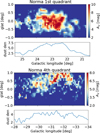 |
Fig. A.1 Skymaps and dust profiles for the spiral arm tangencies for the Norma arm. The top panel displays a skymap in Galactic coordinates (l, b) integrated over a distance range selected by eye (see text), while the bottom panel shows the corresponding dust extinction profile as a function of Galactic longitude within that distance range. |
Appendix B Comparison with map from M06
To highlight the advancements introduced by REDLINE, we compare its performance with the results of Marshall et al. (2006). Both approaches utilise data from 2MASS and are based on the BGM, although the BGM has undergone significant updates since the original analysis (as discussed above). The results from Marshall et al. (2006) were released as a series of distance extinction pairs for a regular grid of sight-lines spaced 15′apart for |l| ≤ 100° and |b| ≤ 10◦. Each sightline had a varying number of bins and there was no fixed distance binning. To compare with the current results, we regrid their results in distance to a regular 100 pc binning using linear interpolation. Their map, between ±1◦, is shown alongside our new results in Fig. B.1.
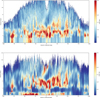 |
Fig. B.1 Comparison between the results of (Marshall et al. 2006) (top) with those of REDLINE (bottom). Both maps are on the same colour scale. The maps are the result of choosing lines of sight in the region |l| <= 100° and |b| <= 1° (corresponding to the overlap of the two maps). The dense structures in the REDLINE maps are more defined than those in M06, and cover a larger distance range. |
Marshall et al. (2006) employed a technique that focused on isolating red giant stars and binning them to infer extinction as a function of distance. While effective, this method restricted the analysis to a specific subset of the stellar population, potentially limiting the resolution and comprehensiveness of the resulting extinction maps. In contrast, REDLINE is based on a custom MCMC that incorporates all stellar types available in the 2MASS dataset. This approach not only maximises the utilisation of the available data but also enhances the robustness and precision of the extinction measurements across different regions of the Galaxy.
The application of REDLINE has resulted in several notable improvements in the extinction maps. Unlike the Marshall et al. (2006) map, which was limited to Galactic longitudes within ±100 degrees, REDLINE extends the extinction mapping to a full 360 degrees in longitude. Structures within the ISM are also more distinctly defined, allowing for a clearer delineation of complex dust distributions. The use of dwarf stars in the RED-LINE distance estimation enables the resolution of nearby ISM features, which were previously less discernible. Furthermore, REDLINE effectively removes the artificial extinction wall at approximately 2 kiloparsecs that was present in the older map. This improvement is also likely due to the use of all stellar types in the MCMC approach.
In regions corresponding to the molecular ring, REDLINE is more able to separate distinct ISM structures. The ability to distinguish multiple overlapping dust features in this complex region is a clear advantage of the REDLINE method. Additionally, the dust lanes around the Galactic centre appear more pronounced.
All Tables
Parameters of the classic spiral arms in the Milky Way as derived from the REDLINE map and compared with the fit from R19.
All Figures
|
Fig. 1 Parameterisation of the problem. Extinction distance pairs are defined with respect to the previous pair. This line of sight extinction distribution requires 12 parameters. Linear interpolation was used to provide a continuous solution along the line of sight. |
| In the text | |
|
Fig. 2 Result of REDLINE in the presence of a single cloud using simulated observations. The diamonds with error bars are the different distance-extinction pairs (left axis), the solid line is the derivative of the extinction with respect to distance, the dashed line is the diffuse extinction, and the dotted lines show the 1 and 2-σ levels (right axis). Here a cloud is clearly detected at 4 kpc, identical to the injected cloud distance. |
| In the text | |
|
Fig. 3 Example lines of sight using real data in a 15′ by 15′ pixel towards prestellar cloud candidates (Planck Collaboration XXVIII 2016). Clockwise from the top left, the panels show one detected cloud (l = 9.25, b = −0.2), two detected clouds (l = 17.2, b = −1.5), no detections (l = 215, b = 4.1), and finally one detected cloud with only an upper limit for the distance (l = 159.7, b = −0.9). Symbols and line styles are as in Fig. 2. The fields shown here were chosen to sample different environments and are not all in the final footprint of the map presented in this paper. |
| In the text | |
|
Fig. 4 REDLINE view of the Galactic plane as seen from the North Galactic Pole. The Sun is at the origin and the Galactic centre is at (x, y) = (8, 0). Dotted circles are plotted every 2 kpc around the solar position, and dashed lines are plotted every 30 degrees. The quantity plotted here is extinction per unit distance, and is proportional to dust density. There is a paucity of dust in the outer Galaxy, and most of the dust is seen to lie in the so-called molecular ring. |
| In the text | |
|
Fig. 5 Local dust overdensities relative to surrounding matter in the REDLINE map. To highlight regions where dust density significantly deviates from the ambient material, the map of the Galactic plane was first lightly smoothed and then a heavily smoothed version was subtracted from it. This technique enhances local density variations, effectively isolating overdense features from the broader background. The overlaid spiral arms are the result of a fit to the data and are explained in Sect. 4.2.2. |
| In the text | |
|
Fig. 6 Top: median interstellar extinction as a function of Galactic radius (blue line) as well as a smoothed version (orange line). Middle: average extinction in the Galactic plane. The solar position is indicated at x = −8, y = 0. Bottom: comparison of our dust density with the H2 mass surface density as a function of Galactic radius from Fig. 7 of Heyer & Dame (2015). Distances have been scaled to R⊙ = 8 kpc and the vertical axes have been arbitrarily scaled. |
| In the text | |
|
Fig. 7 REDLINE results for the entire Galactic plane. The dust density is represented in a 2D longitude–distance plane. Note that this representation stretches structures out horizontally at low distance. (For a polar projection that does not do this see Fig. 4.) |
| In the text | |
|
Fig. 8 Log likelihood of spiral parameters for the four major arms. From the top row to the bottom row, the panels show Norma, Scutum-Crux, Sagittarius-Carina, and Perseus, respectively. The left column shows the density likelihood, the middle column is the tangent likelihood, and the right column is the combination of both. Note that Perseus has no tangents, so the likelihood is flat. |
| In the text | |
|
Fig. 9 Spiral arm structure near tangent points. The figure is arranged in four quadrants with each containing paired images showing longitude-distance relationships (top) and corresponding sky distributions (bottom). Top left: Scutum and Norma arms (first quadrant). Top right: Crux and Norma arms (fourth quadrant). Bottom left: Sagittarius arm. Bottom right: Carina arm. Spiral arm fits (Sect. 4.2.2) are shown as dotted lines, with maser positions and their error bars colour-coded by arm: Norma (magenta), Scutum/Crux (red), and Sagittarius/Carina (green) |
| In the text | |
|
Fig. 10 Same as Fig. 7 but with the results of the spiral arm fitting. Much of the structure of the map can be attributed to this spiral structure; however, there are also a number of exceptions, most notably the dust lanes associated with the Galactic bar. |
| In the text | |
|
Fig. 11 REDLINE overdensity map in greyscale with spiral arm fits from this study (dashed lines) and from Reid et al. (2019) (solid lines) overlaid. Masers from Reid et al. (2019) are also plotted for comparison. In all datasets, colours indicate the corresponding spiral arm or its association, as detailed in the legend. |
| In the text | |
|
Fig. 12 Left: reproduction of the Gaia Collaboration (2023a) OB stellar overdensity map. Centre: dust overdensity (this work) shown with the same Galactic coordinate system for direct comparison. Right: greyscale dust overdensity overlaid with coloured contours of OB stellar overdensity. The red contours highlight regions where stellar features coincide with low-dust zones (white in the background), while the blue contours trace apparent stellar ‘gaps’ that align with high-dust concentrations (dark grey to black in the background). |
| In the text | |
|
Fig. 13 Top: top-down view of the Galactic centre region. The Galactic centre is marked with a star, and the stellar bar, as modelled by the BGM, is indicated by the dashed line. The dotted lines delimit the region selected for the study of the dust lanes. Bottom: sky projection of the dust distribution within the region defined by the dotted lines in the top panel. The longitude range used is indicated by the magenta dashed line in the top panel. The dust lanes exhibit a clear tilt: at negative longitudes, the dust lies above the Galactic plane (b = 0°), while at positive longitudes, it lies below. |
| In the text | |
|
Fig. 14 REDLINE (left) and Bayestar (Green et al. 2019) + DECaPS 3D Dust (Zucker et al. 2025) (right) on the same physical and colour scale. The Sun is at the origin, and the Galactic concentric rings are plotted every 2 kpc and radial lines every 30 degrees. |
| In the text | |
|
Fig. A.1 Skymaps and dust profiles for the spiral arm tangencies for the Norma arm. The top panel displays a skymap in Galactic coordinates (l, b) integrated over a distance range selected by eye (see text), while the bottom panel shows the corresponding dust extinction profile as a function of Galactic longitude within that distance range. |
| In the text | |
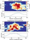 |
Fig. A.2 Same as Fig. A.1 but for the Scutum-Crux tangencies. |
| In the text | |
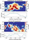 |
Fig. A.3 Same as Fig. A.1 but for the Sagittarius-Carina tangencies. |
| In the text | |
|
Fig. B.1 Comparison between the results of (Marshall et al. 2006) (top) with those of REDLINE (bottom). Both maps are on the same colour scale. The maps are the result of choosing lines of sight in the region |l| <= 100° and |b| <= 1° (corresponding to the overlap of the two maps). The dense structures in the REDLINE maps are more defined than those in M06, and cover a larger distance range. |
| In the text | |
Current usage metrics show cumulative count of Article Views (full-text article views including HTML views, PDF and ePub downloads, according to the available data) and Abstracts Views on Vision4Press platform.
Data correspond to usage on the plateform after 2015. The current usage metrics is available 48-96 hours after online publication and is updated daily on week days.
Initial download of the metrics may take a while.