| Issue |
A&A
Volume 704, December 2025
|
|
|---|---|---|
| Article Number | A59 | |
| Number of page(s) | 11 | |
| Section | Interstellar and circumstellar matter | |
| DOI | https://doi.org/10.1051/0004-6361/202554757 | |
| Published online | 05 December 2025 | |
Low-ionization structures in planetary nebulae
IV. The molecular hydrogen counterpart
1
Universidad Nacional de Córdoba, Observatorio Astronómico de Córdoba,
Laprida 854,
X5000BGR
Córdoba,
Argentina
2
Consejo Nacional de Investigaciones Científicas y Técnicas (CONICET),
Godoy Cruz 2290, CABA, CPC
1425FQB,
Argentina
3
Institute for Astronomy, Astrophysics, Space Applications and Remote Sensing, National Observatory of Athens,
Penteli
15236,
Greece
4
Observatório do Valongo, Universidade Federal do Rio de Janeiro,
Ladeira Pedro Antonio 43,
Rio de Janeiro
20080-090,
Brazil
★ Corresponding author: This email address is being protected from spambots. You need JavaScript enabled to view it.
Received:
25
March
2025
Accepted:
26
August
2025
Context. Low-ionization structures (LISs), found in all morphological types of planetary nebulae (PNe), are small-scale features that are prominent in emission from low-ionization species such as [N II], [S II], [O II], and [O I]. Observational and theoretical efforts aim to better understand their origin and nature. The recent detection of molecular hydrogen (H2) emission associated with LISs in a few PNe has added a new piece to the puzzle of understanding these nebular structures.
Aims. Although observational studies indicate that LISs are characterized by lower electron densities than their host PNe, model predictions suggest that these structures have higher total densities. The detection of H2 emission from LISs in more PNe could help reconcile the observations with model predictions.
Methods. We conducted observations of five PNe with already known LISs using the Near InfraRed Imager and Spectrometer (NIRI) mounted on the 8 m Gemini North telescope. A narrowband filter, centered on the H2 1–0 2.122 µm emission line, was used along with a continuum filter to ensure continuum subtraction.
Results. We present a deep, high-angular-resolution near-IR narrowband H2 1–0 S(1) imaging survey of five Galactic PNe with LISs. We nearly double the sample of LISs detected in the H2 1–0 2.122 µm emission line, as well as the number of host PNe. These findings allow us to demonstrate that the systematically lower electron density in LISs – relative to the rims and shells of their host nebulae – is linked to the presence of H2 molecular gas. Furthermore, we provide the first estimate of the excited H2 molecular mass in LISs, which is between 200 and 5000 times lower than the corresponding ionized gas mass.
Key words: ISM: jets and outflows / ISM: molecules / photon-dominated region (PDR)
© The Authors 2025
 Open Access article, published by EDP Sciences, under the terms of the Creative Commons Attribution License (https://creativecommons.org/licenses/by/4.0), which permits unrestricted use, distribution, and reproduction in any medium, provided the original work is properly cited.
This article is published in open access under the Subscribe to Open model. This email address is being protected from spambots. You need JavaScript enabled to view it. to support open access publication.
1 Introduction
As a low- or intermediate-mass star consumes its fuels and approaches the end of its evolutionary life, it ejects its outer layers into the interstellar medium, leaving behind a hot and luminous core. The radiation field of the exposed core peaks in the ultraviolet (UV) range, resulting in the dissociation of molecular gas formed in the previous asymptotic giant branch (AGB) stage and in the subsequent ionization of atomic gas. These processes form the bright and colorful planetary nebulae that we observe, which are among the most important contributors to the chemical enrichment of the interstellar medium in galaxies.
Planetary nebulae (PNe) display a variety of shapes and morphologies, such as round, elliptical, bipolar, and multipolar forms (e.g. Manchado et al. 1996). They are also characterized by distinct components such as rims, shells, and attached halos, which are prominent mostly in [O III] and hydrogen recombination lines (Balick & Frank 2002). In addition, PNe display smaller-scale structures that are prominent in emission from low-ionization species such as N+, S+, O+, or O0 (e.g., Corradi et al. 1996; Balick et al. 1998; Gonçalves et al. 2001).
Many efforts have been made to decipher the nature of these low-ionization structures (hereafter LISs) and their unexpectedly low electron density relative to the surrounding gas (see e.g., Balick et al. 1994; Hajian et al. 1997; Gonçalves et al. 2003, 2004, 2009; Akras & Gonçalves 2016; Danehkar et al. 2016; Ali & Dopita 2017; Monreal-Ibero & Walsh 2020; Miranda et al. 2021; Akras et al. 2022; Mari et al. 2023b). Recently, Mari et al. (2023a) investigated the physicochemical properties of LISs and their host PNe by conducting a statistical analysis of a sample of 33 PNe containing 88 rims and/or shells and 104 LISs, and verified that neither the chemical abundances nor the electron temperatures show significant differences between the components. However, LISs correspond to a group of nebular structures that are statistically different from the rims and attached shells of the host nebula in terms of electron density (ne), having ne two-thirds lower (∼1700 cm−3) than other nebular components (∼2700 cm−3), with interquartile ranges (25th to 75th percentiles) of 800–2700 cm−3 and 1800–5000 cm−3, respectively.
O’Dell & Handron (1996) discussed the origin of cometary knots in the well-studied Helix nebula, suggesting that Rayleigh–Taylor instabilities during the early PN phase are the most likely cause, although a primordial origin linked to the central star’s formation cannot be excluded. Other authors have also suggested similar formation mechanisms to explain the origin of LISs, such as stagnation points (Steffen et al. 2001), Rayleigh-Taylor instabilities (e.g., Ramos-Larios & Phillips 2009), and AGB fossils (e.g., Gonçalves et al. 2001), among others. All these models require LISs densities that are orders of magnitude higher than those of the surrounding nebular gas, typically >104 cm−3 (e.g., Raga et al. 2008; Balick et al. 2020). Gonçalves et al. (2009), in an attempt to reconcile optical observations with theoretical models, proposed that a significant fraction of gas in LISs should be neutral (atomic and/or molecular) and thus hidden for visible-light observational studies.
A high total density (i.e., electron, neutral and molecular) is a necessary condition for preventing molecular hydrogen (H2) dissociation. The presence of H2 in PNe is well established, particularly in bipolar PNe (Gatley’s rule, e.g., Kastner et al. 1996), primarily through observations of the ro-vibrational emission line H2 v=1–0 S(1), centered at 2.122 µm. The Helix nebula, one of the brightest and closest planetary nebulae to Earth, was among the first to provide evidence of H2 associated with knotty structures, enabling comprehensive investigations of its cometary knots through both observational and modeling approaches (O’Dell & Handron 1996; O’Dell et al. 2000; López-Martín et al. 2001; Meixner et al. 2005; Hora et al. 2006; Matsuura et al. 2009).
More recently, the presence of H2 has also been verified in other microstructures embedded in PNe, such as LISs. In this context, it should be noted that an empirical linear correlation between the [O I] λ6300 and H2 1–0 S(1) emission lines was already demonstrated in early studies of PNe (Reay et al. 1988). Following the link between these two lines, Akras and collaborators selected LISs with strong [O I] λ6300 emission and have successfully detected the H2 2.122µm line in several cases: K 4-47 and NGC 7662 (Akras et al. 2017), as well as NGC 6543 and NGC 7009 (Akras et al. 2020). Two additional PNe with H2-emitting knots have also been reported, namely Hu 1-2 (Fang et al. 2015) and Hb 12 (Fang et al. 2018).
Aleman & Gruenwald (2011) showed that H2 is confined to a narrow region between the point where the ionized hydrogen fraction reaches 95% and the outer boundary of the ionized region, where this fraction drops to 0.01%. Within this transition zone, the peak emissivity of the H2 2.122 µm line is found, together with those of low-ionization lines ([N II], [S II], and [O I]) (see their Fig. 4), with spatial separations that exceed the thickness of the ionization front. More recently, Akras et al. (2024) present the first spatially resolved MUSE (Multi-Unit Spectroscopic Explorer, mounted at the Very Large Telescope of the European Southern Observatory) image of the atomic carbon line [C I] 8727 Å in NGC 7009. This line originates only from pairs of LISs, suggesting the presence of high-density, partially ionized gas. The same emission line has also been detected in the LISs of NGC 3242, suggesting that it could be another common characteristic of these microstructures (Konstantinou et al. 2025). García-Rojas et al. (2022) also present a [C I] 8727 Å MUSE map for a number of PNe. Examining the radial stratifi-cation of emission lines in the K1 LIS of NGC 7009 (Gonçalves et al. 2003), Akras et al. (2024) argue that the photoevaporation of dense knots could explain the observations.
The ionization and photoevaporation of neutral clouds illuminated by the UV radiation of O and/or B stars have been studied since the mid-20th century (Kahn 1954; Oort & Spitzer 1955), with the aim of explaining their acceleration. Years later, Bertoldi (1989); Bertoldi & McKee (1990) developed approximate analytical models for the evolution of neutral clouds. Photoevaporation of the gas in these clouds results in a rocket effect, causing the clouds to accelerate away from the ionizing source. In such neutral or molecular clouds, the ionization and photodissociation fronts are not necessarily separated, which is a key difference from classical photodissociation regions (PDRs) (Bertoldi & Draine 1996; Henney et al. 2007). Subsequently, several theoretical and observational studies applied the photoe-vaporation mechanism to neutral clumps in PNe (e.g., Mellema et al. 1998; Raga et al. 2005) and to the cometary knots in the Helix nebula (e.g., O’Dell et al. 2000; López-Martín et al. 2001; O’Dell et al. 2005). Nevertheless, LISs in PNe that do not show cometary morphology remain poorly understood, and the H2 molecular component has only been confirmed observationally in a handful of cases.
This pilot survey presents the H2 emission line of a sample of LISs in PNe, covering a variety of LISs types in PNe of different morphological classes. The main goal of this study is to analyze and quantify the molecular H2 gas content of LISs. The detection of H2 emission exclusively associated with LISs also allows for comparison between the masses of ionized and molecular material. Such an analysis can provide a more accurate estimate of the molecular mass, at least in its excited state, within the LISs. Through this approach, we aim to advance the understanding of a key discrepancy: whereas theoretical models predict significantly higher total densities in LISs compared to the rims or shells of their host PNe, optical observations indicate that the electron densities in LISs are at least two-thirds lower than those of the surrounding gas. This study will help narrow the gap between models and observations, providing crucial data to resolve this intriguing dichotomy.
In Section 2, we present the observed sample along with the data reduction and calibration. In Section 3, we show the results obtained from NIRI images. Section 4 provides the mass estimates and the relationship between ionized and excited molecular content. Finally, in Sections 5 and 6, we present the discussion and overall conclusions.
2 Narrowband imaging observations
To test the hypothesis that the presence of H2 is a general characteristic of LISs, and is therefore associated with different LISs classes – knots, filaments, and jets, whether in pairs or isolated – we conducted very deep narrowband H2 2.122 µm imaging for a sample of five PNe. Observations were carried out with the Near-InfraRed Imager and Spectrometer (NIRI), mounted on the 8 m Gemini North telescope at Mauna Kea, Hawaii.
2.1 Data acquisition and reduction
The observations were obtained between July and October 2020 (Program ID: GN-2020B-Q-128, PI: S. Akras). The f/6 configuration, with a pixel scale of 0.117 arcsec and a filed of view (FoV) of 120 arcsec, was used since it is ideal for observing PNe with angular sizes smaller than 100 arcsec. The narrowband G0216 filter, with an effective width of ∼327 Å, centered at 2.1239 µm, was used to isolate the H2 1–0 S(1) line at 2.122 µm. For proper continuum emission subtraction, the G0217 filter, with an effective width of ∼329 Å, centered at 2.0975 µm, was also employed. To increase the signal-to-noise ratio (S/N), several individual frames were obtained per object. The observations are detailed in Table 1. In agreement with the Gemini baseline calibrations, GCAL (Gemini Facility Calibration Unit) flat frames and dark frames with different times based on science images were obtained to correct thermal emission, dark current, and hot pixels. Standard stars (SAO34401, GSPC S813-D, FS 150, and FS 123) were also observed to flux-calibrate the data.
Before starting data reduction, and as recommended by Gemini1, we applied the PYTHON routines CLEARIR.py and NIRLIN.py. The CLEARIR.py routine removes artifacts such as vertical striping and/or horizontal banding, while NIRLIN.py. corrects the nonlinearity of the detector. The images were reduced using DRAGONS2 (Data Reduction for Astronomy from Gemini Observatory North and South, Labrie et al. 2019), a PYTHON-based software package for Gemini data reduction, provided by the Gemini observatory. This package stacks multiple dark observations to create a master dark. A bad pixel mask (BPM) was generated from the GCAL flats and short darks, and a master flat was generated from multiple observations with lamps-on and lamps-off. The science data were then reduced using the BPM, the corresponding master dark, and the appropriate master flat field for each filter.
Observation log.
2.2 Flux calibration and continuum subtraction
Owing to nighttime atmospheric variations, the full width at half maximum (FWHM) of the background stars was not always identical in both filters. Using background stars present in both images, we computed the average FWHM for each target. The image with the smallest FWHM was degraded before subtracting the continuum from the emission-line image. This was performed using the GAUSS task in IRAF (Image Reduction and Analysis Facility, Tody 1986), which convolves the image with an elliptical Gaussian function after specifying the sigma parameter.
Due to the lack of broadband K filter observations for the standard stars, we calculated their theoretical K magnitudes (FluxK theoretical) by modeling their blackbody spectral energy distributions (SEDs). For this purpose, we adopted effective temperatures derived from their spectral types and applied the transmission curves of the filters. For flux calibration, we used the absolute K magnitudes of the standard stars (FluxK standard star) from the Two Micron All Sky Survey (2MASS; Skrutskie et al. 2006) for SAO34401 and from the UKIRT Infrared Deep Sky Survey (UKIDSS; Hambly et al. 2008) for GSPC S813-D, FS 150, and FS 123. From these values, we derived calibration factors (FluxK standard star/FluxK theoretical), which were then used to flux-calibrate the narrowband images of the targets obtained with NIRI, applying the transmission curves of the corresponding filters.
For continuum subtraction in the flux-calibrated images, we first aligned the H2 and K-cont images, using as many field stars as possible. We then computed the scale factor required to properly subtract field stars from the emission-line frames. Specifically, we applied the equation  , where (H2/K−cont) represents the scale factor. The scale factor was estimated by comparing the fluxes of background stars present in both images. Fig.1 shows an example of the continuum-subtraction process using different scale factors. Too small scale factor is barely perceptible in the continuum subtraction, while excessively large values lead to oversubtraction and an underestimation of the H2 fluxes.
Several uncertainties affect this process, including: (i) the standard stars effective temperature used to obtain their theoretical SEDs; (ii) the conversion factors applied for the flux calibration of both standard stars and science targets; and (iii) the scale factor used for continuum subtraction, determined by ensuring satisfactory removal of field stars in the H2 science images. The flux calibration is additionally subject to an inherent photometric uncertainty of approximately 10% due to unmeasured atmospheric extinction3. Each of these processes contributes an uncertainty of roughly 10%, although they may not be entirely independent. In addition, both 2MASS and UKIRT report photometric errors of approximately 0.02–0.03 mag (Skrutskie et al. 2006; Lawrence et al. 2007, respectively), corresponding to a baseline flux calibration uncertainty of around ∼3%. The combined effect of these uncertainties results in an overall uncertainty of about 30–40% in the H2 flux measurements.
Despite these uncertainties, our comparison of parameter A in the relation  with values from the literature shows a difference of only 13% (see Section 4.2, where we define and discuss the H II over H2 mass ratio). This level of agreement suggests that, despite significant uncertainties, our flux calibration methodology yields reliable results.
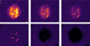 |
Fig. 1 Comparison of continuum-subtracted images obtained with different scale factors. From top to bottom and left to right, the scale factor increases (0.9, 1.0, 1.05, 1.1, 1.2, 1.3). Initially, poor continuum subtraction is evident, as the field stars appear as H2 line emitters (top panels). The final two bottom panels provide clear examples of over-subtraction of the continuum. |
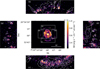 |
Fig. 2 Surface brightness (SB) of the H2 1–0 S(1) continuum-subtracted image for NGC 2392 (center). Panels a-d display the H2 continuum-subtracted image overlaid with HST [N II] emission contours for different nebular regions. |
3 Comparison of NIRI H2 and HST [N II] imagery
We present the first deep, spatially resolved, continuum-subtracted narrowband H2 2.122 µm images of the planetary nebulae NGC 2392, NGC 6751, NGC 6818, NGC 6884, and NGC 7354. The NIRI H2 data are compared with HST [N II] images of this PNe sample, which facilitates the interpretation of the results.
NGC 2392. In addition to the multiple knotty and filamentary LISs located in the inner part of its high-excitation shell, NGC 2392 also hosts a bipolar jet with a velocity of 150–185 km s−1, directed almost directly toward the observer (O’Dell & Ball 1985; Gieseking et al. 1985). Because of their orientation and low surface brightness, these jets are not detected in optical images and can only be distinguished in spatially resolved, high-resolution [N II] spectra ( e.g., García-Díaz et al. 2012; Guerrero et al. 2021). The central panel of Fig. 2 shows the narrowband continuum-subtracted H2 2.122 µm image of NGC 2392. Multiple knots and filaments are detected in the molecular hydrogen light. Panels (a)–(d) show different regions of the nebula, displaying HST [N II] λ6584 emission contours, overlaid on the NIRI H2 1–0 S(1) image of NGC 2392. A strong spatial correlation between the H2 and [N II] lines is evident, consistent with previous findings (Akras et al. 2017, 2020). The H2 fluxes of five LISs are listed in Table 2, ranging from 0.25 to 0.8 × 10⁻¹⁵ erg s−1 cm−2.
NGC 6751. Among its multitude of structures, this PN has a [N II] knotty ring and irregular filaments in the northeast quadrant of the halo (Chu et al. 1991; Clark et al. 2010). Figure 3 presents the continuum-subtracted H2 images of NGC 6751. The emission of H2 emanates from the inner parts of the nebula, where [N II] emission is evident. Faint H2 emission is detected in the pairs of jet-like structures, which are also detected in the [N II] line. The H2 fluxes of the latter structures vary from 0.37 to 1.73 × 10⁻¹⁵ erg s−1 cm−2 (see Table 2). The filamentary structures of the halo exhibit stronger H2 emission (upper left panel), with fluxes ranging from 1.85 to 3.84 × 10⁻¹⁵ erg s−1 cm−2. These findings further support the Clark et al. (2010) idea that such filaments are remnants of AGB mass-loss events.
NGC 6818. In [N II] emission, NGC 6818 exhibits multiple filamentary structures distributed across the whole nebula, labeled as “mustaches” by Benetti et al. (2003). Figure 4 presents our deep near-IR image of this nebula, together with the [N II] emission line contours from HST. The H2 2.122 µm emission line is detected only in the LISs or “mustaches”, prominent in [N II]. The H2 flux from three LISs varies between 1.44 and 2.88 × 10⁻¹⁵ erg s−1 cm−2 (see Table 2), placing them among the brightest LISs in our sample.
NGC 6884. The [N II] image of NGC 6884 reveals a pair of LISs in opposite directions, with a radial velocity of 40 km s−1 (Miranda et al. 1999), originally interpreted as precessing bipolar outflows. More recent diffraction-limited, narrowband HST images in the [N II] emission revealed that the pair of knots consists of two symmetrical, knotty, arc-shaped structures (Palen et al. 2002). Figure 5 presents the continuum-subtracted H2 2.122 µm image of NGC 6884. In the left panel, significant H2 is detected in the outer halo of this nebula, at distances of 30–40 arcsec from the central star. Panels (a) and (b) show a zoom-in view of the central part of the nebula, where an arc-like structure is clearly detected in the eastern part. The H2 (1–0) S(1) emission from this arc-like structure shows a spatial correlation with the [N II] emission in the HST data, but the lower spatial resolution of our data prevents us from verifying whether H2 emission originates from the knots. The H2 flux in two regions of the eastern arc-like structure ranges from 0.75 to 1.86 × 10⁻¹⁵ erg s−1 cm−2 (see Table 2), while regions in the outer halo exhibit fluxes between 2.60 and 18.35 × 10⁻¹⁵ erg s−1 cm−2. As in NGC 6751, the H2 emission from halo structures in this object also appears to be related to remnants of mass-loss episodes during the AGB stage.
NGC 7354. Multiple microstructures prominent in [N II] emission have been identified and studied in NGC 7354 (e.g., Hajian et al. 1997; Contreras et al. 2010), including a pair of jet-like LISs along its major axis. Phillips et al. (2009) studied NGC 7354 using near- and mid-IR data from 2MASS and Spitzer. However, due to the low spatial resolution of their data, the equatorial LISs and jet-like structures were not clearly detected. Nevertheless, all LISs are detected in our data (Fig. 6). The left panel presents the continuum-subtracted H2 image of NGC 7354. The right panels a, b, c, and d show the contours of [N II] emission superimposed on the H2 zoom-in images of the LISs. There is a clear spatial correlation between the two emission lines. We also report the first detection of H2 emission from the jet-like structures, indicative of collisional excitation. The H2 fluxes of four LISs vary from 1.35 to 2.68 × 10⁻¹⁵ erg s−1 cm−2 (see Table 2).
Position, H2 1–0–S(1) fluxes, and molecular masses for various LISs in the studied PNe.
4 Molecular and ionized content of LISs
The primary motivation for studying the emission of LISs in molecular hydrogen lines was to understand why the vast majority of LISs exhibit electron densities lower than those of nebular rims and shells. Since this finding contradicts theoretical predictions, we computed the molecular and ionized masses in LISs to examine whether their H2 content helps alleviate the tension between observations and theory, as suggested by Gonçalves et al. (2009). In this section, we integrate our results with data published in the literature.
4.1 Molecular hydrogen mass
After measuring the H2 λ2.122 fluxes for several LISs in our sample, we estimated their molecular hydrogen mass. For this purpose, we adopted Equation (1) from Scoville et al. (1982):
 (1)
where nH2 is the H2 volume density, VH2 is the volume of the region that contains the H2 gas, AS(1) = 3.47 × 10⁻⁷s−1 is the H2 1–0 S(1) transition probability for temperature T=2000 K (Turner et al. 1977; Riffel et al. 2008), fν=1,J=3 = 0.0122 is the population fraction of H2 in the ν=1, J=3 level, d is the distance of the nebula, h is Planck constant, and ν is the frequency of the H2 line. Rearranging the above equation allowed us to determine the mass of the H2 component in LISs, which can be written as
(1)
where nH2 is the H2 volume density, VH2 is the volume of the region that contains the H2 gas, AS(1) = 3.47 × 10⁻⁷s−1 is the H2 1–0 S(1) transition probability for temperature T=2000 K (Turner et al. 1977; Riffel et al. 2008), fν=1,J=3 = 0.0122 is the population fraction of H2 in the ν=1, J=3 level, d is the distance of the nebula, h is Planck constant, and ν is the frequency of the H2 line. Rearranging the above equation allowed us to determine the mass of the H2 component in LISs, which can be written as
![$\matrix{{{M_{{{\rm{H}}_2}}} = {{2{m_p}{F_{{{\rm{H}}_{\rm{2}}}\lambda 2.122}}4\pi {d^2}} \over {{f_{v = 1,J = 3}}{A_{S(1)}}hv}}} \hfill \cr {\~5.0776 \times {{10}^7}\left( {{{{F_{{{\rm{H}}_{\rm{2}}}\lambda 2.122}}} \over {{\rm{erg}}\,{{\rm{s}}^{ - 1}}{\rm{c}}{{\rm{m}}^{ - 2}}}}} \right){{\left( {{d \over {kpc}}} \right)}^2}[{M_ \odot }],} \hfill \cr }$](/articles/aa/full_html/2025/12/aa54757-25/aa54757-25-eq4.png) (2)
where mp is the mass of the proton and FH2 λ2.122 is the observed flux of the emission line (Diniz et al. 2015).
(2)
where mp is the mass of the proton and FH2 λ2.122 is the observed flux of the emission line (Diniz et al. 2015).
Since an external energy source is required to excite the ro-vibrational levels of the H2 molecule, such as UV photons from the central star or shock waves, the flux from the H2 λ2.122 line does not represent the distribution of the cold molecular component. Consequently, our data trace the highly excited H2 gas, referred to as the “warm” H2 component, and therefore the masses estimated from Equation (2) correspond to this component. Thus, the computed masses presented in this work represent the lower limits of the total H2 mass in LISs.
Table 2 presents the first estimations of the warm H2 masses for 19 LISs in our sample of five PNe. These masses range from 0.4 to 10×10−7 M⊙, with an average of 4.6×10⁻⁷ M⊙. Given that Equation (2) is commonly applied to AGN (e.g., Reunanen et al. 2002; Diniz et al. 2015), we also computed the H2 mass of the cometary knot K1 (RA:22:29:33.41, Dec:–20:48:04.73) in the Helix planetary nebula using the same equation to ensure the reliability of our estimates. This procedure resulted in a H2 mass for K1 of ∼3.9×10⁻⁸ M⊙ that is one order of magnitude smaller than the H2 masses in the LISs of our PNe sample. Nevertheless, our measurement of the H2 mass for K1 is in reasonable agreement with that of Matsuura et al. (2007) obtained through near-IR IFU observations (see Table 2). The detection of several H2 lines from different ro-vibrational states allowed the authors to construct an excitation diagram and determine the excitation temperature and column density of the H2 gas, resulting in ∼2 × 10⁻⁸ M⊙, which is half of the value we obtain. Considering the different types of data, the uncertainties in the H2 fluxes, (discussed in Section 2.2) and the fact that we adopted the distance to the nebula from Gaia DR3 parallaxes (Gaia Collaboration 2023; Bailer-Jones et al. 2021) only available more recently, we argue that our methodology provides adequate and reliable warm H2 masses for the LISs.
Wesson et al. (2024) provided an H2 mass for the globules of NGC 6720, using data from the JWST Early Release Observations. They used the same approach as De Marco et al. (2022) for NGC 3132. The extinction of the knots in the IR wavelength regime was derived using the extinction law from Cardelli et al. (1989). This led first to the estimation of the column density, and subsequently the total H density and H2 mass. Wesson et al. (2024) estimated densities of nH ∼ 105 cm−3 and H2 masses of ∼10−6 M⊙. They noted that at these densities  , the globules could be in pressure equilibrium with the surrounding ionized gas. Consequently, the globules could remain essentially stable, avoiding collapse or dissipation until the surrounding gas recombines. In contrast, De Marco et al. (2022) report a higher density of nH∼106 cm−3 and an H2 mass of ~10−5 M⊙ for the filaments in NGC 3132. These values are two to three orders of magnitude higher than the mass of the cometary knot in Helix, and one to two orders of magnitude greater than our masses in LISs. Although an in-depth comparison of the different structures studied in the cited works is beyond the scope of this study, we argue that the methodology followed by Matsuura et al. (2007) provides robust estimates of densities and masses.
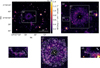 |
Fig. 3 Surface brightness of the H2 1–0 S(1) continuum-subtracted image for NGC 6751. The upper left panel displays the entire nebula, revealing faint emission from its halo at distances greater than 30 arcsec. The right panel a provides a zoomed-in view of the nebula’s center, showing the eastern and western jet-like structures along with numerous knots in the outer rim. The bottom panels present the continuum-subtracted H2 image overlaid with HST [N II] emission line contours: panel c focuses on the nebula’s center, while panels b and d display the pairs of jet-like structures. The apparently bright knot in the western jet-like structure is a background star. |
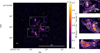 |
Fig. 4 Surface brightness of the H2 1–0 S(1) continuum-subtracted image for NGC 6818 is shown in the left panel. The other panels present the H2 continuum-subtracted image overlaid with HST [N II] emission contours, highlighting three regions of the nebula: panels a and b correspond to the “mustache” structures, while panel c shows the brighter southern part of the nebula. |
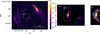 |
Fig. 5 Surface brightness of the H2 1–0 S(1) continuum-subtracted image for NGC 6884 is shown in the left panel. The center panel provides a zoomed-in view of the entire nebula, while the other panel present the H2 continuum-subtracted image overlaid with HST [N II] emission contours, highlighting the knotty, arc-like structure in one half of the nebula, labeled as panel b. |
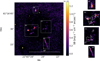 |
Fig. 6 Surface brightness of the H2 1–0 S(1) continuum-subtracted image for NGC 7354 is shown in the left panel. The other panels present the H2 continuum-subtracted image overlaid with HST [N II] emission contours, highlighting four regions of the nebula: panels a and d correspond to the pair of jet-like structures, while panels b and c show the equatorial bright LISs. |
4.2 Ionized mass
In addition to the warm H2 component, the ionized mass can be estimated using near-IR observations, specifically from the flux of the Brγ emission line:
 (3)
(3)
Assuming that the H II region associated with the H2 is optically thin in Brγ (Scoville et al. 1982), and adopting case B emissivities from Osterbrock & Ferland (2006), the ionized mass (MHII) can be derived using the equation
![${M_{HII}}\~3.29 \times {10^{13}}\left( {{{{F_{Br\gamma }}} \over {{\rm{erg}}\,{{\rm{s}}^{ - 1}}{\rm{c}}{{\rm{m}}^{ - 2}}}}} \right){\left( {{d \over {{\rm{kpc}}}}} \right)^2}{\left( {{{{n^e}} \over {{\rm{c}}{{\rm{m}}^{ - 3}}}}} \right)^{ - 1}}[{M_ \odot }]$](/articles/aa/full_html/2025/12/aa54757-25/aa54757-25-eq7.png) (4)
(Storchi-Bergmann et al. 2009).
(4)
(Storchi-Bergmann et al. 2009).
The PNe in our sample were not observed in the Brγ emission line. We therefore adopted the results of Akras et al. (2017, 2020), which provide fluxes for several LISs in four PNe, for both the H2 1–0 S(1) and Brγ lines, ranging from 0.72 to 21.89 × 10⁻¹⁵ erg s−1 cm−2, and from 0.96 to 94.70 × 10⁻¹⁵ erg s−1 cm−2, respectively. In Table A.1, we list the masses for the warm H2 gas (obtained from Equation (2)), as well as the ionized mass (from Equation (4)).
The derivations of these masses for a reasonable number of LISs allow the construction of the  versus MH II diagram and also enable further exploration of the measurements from Akras et al. (2017, 2020). Nebular components from the PN K 4-47, marked with red dots in Fig. 7, deviate significantly from the bulk of the data and were excluded from both the best-fit mass correlation and subsequent discussion. K 4-47 is a highly collimated PN with a pair of LISs located at the tips of its outflows. Photoionization and shock models indicate that these LISs are likely shock-heated, with shock velocities ≥ 150 km s−1 (Corradi et al. 2000; Gonçalves et al. 2004). In the statistical analysis of LISs and host PNe carried out by Mari et al. (2023a), K 4-47 frequently appears as an outlier – in terms of electron temperatures, chemical abundances, and various emission line ratios – showing significant differences from the rest of the LISs.
A significant dispersion (R2 ∼ 0.48) is present in the  relation, which probably reflects the large uncertainties in the masses. The best-fit line is represented by
 (5)
(5)
The median MHII for LISs in Table A.1, excluding K 4-47, is 7.0 × 10⁻⁴ M⊙. Using this value in Equation (5), we obtain  , while the median for this quantity is 3.0 × 10⁻⁷M⊙. According to Matsuura et al. (2007), extinction affects the absolute intensity by less than 5%, which does not impact our results or overall conclusions, given that the uncertainties in our mass estimates are larger. Moreover, following Scoville et al. (1982) and using Equations (1) and (3) for the data in Table A.1, we obtain
 (6)
(6)
This corresponds to a difference of only 13 percent compared to Scoville’s ratio (see their Eq. (8)). Considering the  ratio, which ranges from ∼0.70 to 17.82, and the median electron density of 2325 cm−3 for the LISs in the sample (excluding K 4-47), we find that their ionized masses (MHII) are between approximately 200–5000 times larger than the warm molecular hydrogen masses
  .
.
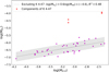 |
Fig. 7 Correlation between ionized and warm molecular hydrogen mass for the LISs in NGC 7662, NGC 7009, and NGC 6543 (Akras et al. 2017, 2020). The gray shaded area represents the uncertainty of the regression line. Outflows from K 4-47 and LISs were excluded from the linear fit due to their significant deviation from the bulk. Red points correspond to these nebular components, with the more massive ones representing the outflows. |
5 Discussion
This work presents the first near-IR H2 1–0 2.122 µm detections in the LISs of NGC 2392, NGC 6751, NGC 6818, NGC 6884, and NGC 7354. We begin by briefly characterizing these structures, where warm molecular hydrogen is detected.
- (i)
A multiple system of knotty and filamentary LISs is located at the inner part of the shell, in the high-excitation PN NGC 2392. This nebula also displays high-velocity ([N II]) jets directed toward the observer but undetected in H2 (García-Díaz et al. 2012; Guerrero et al. 2021). The electron densities of the knots and filaments are 900–1000 cm−3, two to three times lower than those of the nebula shell, while Te does not vary significantly (Barker 1991; Zhang et al. 2012).
- (ii)
Although NGC 6751 displays a large halo in which H2 is also detected (Clark et al. 2010), the clumpy LISs of its inner regions, including the jet-like structures (ansae, in Chu et al. 1991), are the main focus here. The Te is similar across the different nebular regions. In contrast, jet-like structures, knots and rim have densities of ∼200 cm−3, ∼1600 cm−3, and ∼2500 cm−3, respectively (Chu et al. 1991).
- (iii)
NGC 6818 contains multiple [N II]-bright filamentary structures distributed throughout the nebula (“moustaches”, Benetti et al. 2003), which are also observed in H2. These structures are peculiar due to their higher kinematic gradients (Hyung et al. 1999) and electron densities compared to the other nebular components. Across the nebula, ne[S II] varies between 1500 and 2800 cm−3, with the equatorial filamentary structures representing the densest regions (Benetti et al. 2003; Tsamis et al. 2003; Pottasch et al. 2005).
- (iv)
The LISs of NGC 6884 form a pair of knotty, arc-like structures, as revealed by [N II] HST (Palen et al. 2002) and H2 NIRI images. The Te shows a slight variation between the low- (~8500 K) and moderate-ionization (∼10 000 K) regions of the nebula. The low-ionization regions have ne[O II] of ∼16 000 cm−3, whereas, based on [A IV] and [Cl III] diagnostics, the rest of the nebula has values of ∼ 6000 cm−3 (Hyung et al. 1997).
- (v)
The equatorial knots and jet-like structures of NGC 7354, detected in H2, were studied by Hajian et al. (1997); Contreras et al. (2010), who derived their temperatures and densities. The pair of jet-like structures, equatorial knots, and high-ionization shell are characterized by ne (Te) values of ~970 cm−3 (10 000–12 000 K), ∼3000 cm−3 (10 000–13 000 K), and 1500–2600 cm−3 (∼10 000–13 000 K), respectively.
Regardless of their physical conditions, the nebular components, or LISs, in which H2 emission is unambiguously detected, are associated with structures prominent in the [N II] emission line. In most cases, the H2 detections correspond to structures that, relative to the rims and shells of their host nebulae, have lower electron densities. Thus, by doubling the sample of known PNe with the LISs detected in the H2 line, we verify that the LISs are indeed composed of a partially ionized and excited molecular gas. In addition to the LISs, which were the main focus of this narrowband survey, H2 emission was also detected for the first time in the halos of NGC 6751 and NGC 6884.
For the first time, the molecular mass of excited (warm) H2 gas in LISs has been estimated for our sample of five PNe, together with LISs in four PNe reported in the literature. The corresponding ionized masses of these LISs were also calculated. Based on the range of near-IR H2 and Brγ fluxes reported by Akras et al. (2017, 2020), we find that the ionized mass in LISs is between 200 and 5000 times greater than the excited molecular mass.
As mentioned in Section 4, our data do not represent the distribution of the cold molecular component, but only the warm component. The H2 mass of the cold counterpart is commonly estimated through CO emission. However, this method requires converting the CO column density into H2 mass, which in turn requires assuming a conversion factor for the CO/H2 ratio – a highly uncertain quantity (see, e.g., Bolatto et al. 2013).
No direct measurements of the mass of the cold components are available for the LISs discussed in the present work due to the lack of any CO detection so far. Andriantsaralaza et al. (2020) analyzed ALMA CO observations of a globule in the Helix nebula, specifically the C1 globule previously detected in CO and H2 by Huggins et al. (2002). Using CO emission lines as H2 tracers, the molecular mass of the globule head has been estimated as (0.8–1.3)×10−5 M⊙ (Andriantsaralaza et al. 2020) and ⪆1×10⁻⁵M⊙ (Huggins et al. 2002), assuming a CO/H2 ratio of ∼10−4 Huggins et al. (1992, 2002). Considering the H2 2.122 µm flux reported by Huggins et al. (2002) at the globule head (the tail being significantly fainter in this emission), we estimate the warm molecular mass using Equation (2) to be ∼1.5 × 10⁻⁸ M⊙. This suggests that the cold H2 mass in the C1 head is approximately 5.3–8.7 × 10² times greater than the warm H2 mass, yielding a mean ratio of Mcold/Mwarm∼ 7×10². Based on this, if a cold H2 gas component is present in our sample of LISs, their masses should range between (0.3–7.3) × 10−4 M⊙, with a mean value of 3.8×10⁻⁴ M⊙. This value is approximately half of the median ionized mass found for LISs in Section 4.2.
As no other LISs have been detected in both H2 and CO to date, direct comparisons are not possible. Nevertheless, the cold H2 mass in NGC 3132 has been computed from Submillimeter Array (SMA) observations, ranging between ~0.015 and ∼0.15 M⊙, assuming a CO/H2 conversion factor between 10−4 and 10−5 (Kastner et al. 2024).
The presence of molecular gas in LISs offers new insight into their origin and nature. The new detections of H2 emission from LISs double the number of PNe with LISs directly associated with warm molecular gas, bringing the total to nine. This provides further support for the scenario in which LISs may represent mini-photodissociation regions (PDRs) illuminated by hard UV radiation from the central stars of PNe. Nevertheless, the potential PDRs at the surfaces of LISs may differ from the PDRs those typically found in high-mass star-forming regions (Hollenbach & Tielens 1997). The very low ionization parameters of PNe LISs may cause the ionization and dissociation fronts of H2 to merge (Bertoldi & Draine 1996; Henney et al. 2007).
The survival of molecular gas in these nebular structures requires explanation, as it must withstand dissociation by the energetic UV photons emitted by the central star. Recent detection of the [C I] λ8727 emission line from the LISs of NGC 7009 (Akras et al. 2024) and NGC 3242 (Konstantinou et al. 2025) suggests photoevaporation of the molecular gas, which becomes dissociated and ionized as it flows away from the knots. Akras et al. (2024) demonstrated that the northeastern LIS of NGC 7009 exhibits a stratified ionization structure at the interface between the outer ionized gas and the dense molecular core (i.e., within a transition zone). The emission profiles of this LIS show [C I] arising between [N II] and H2, which contrasts with what is observed in PDRs of star-forming regions (e.g., Henney 2021).
As mentioned above, the physical conditions in LISs may deviate significantly from those of typical high-mass star-forming PDRs. Nevertheless, LISs appear to preserve some key features of typical PDRs, such as stratified emission regions, high total densities, and low temperatures. Hollenbach & Tielens (1997) presented a schematic of a PDR structure, in which the H II component is followed by a thin H II/H I layer that absorbs Lyman-continuum photons. These layers are followed by large column densities of O, C, C+, CO, and vibrationally excited H2. The typical total densities (103−5 cm−3) and temperatures (between 200 and 1000 K) of PDRs are comparable to those predicted by Balick et al. (2020), who report high densities (106−7 cm−3) and low temperatures (3×100−3 K) in the interior of LISs. Such high densities are also suggested for the LISs in NGC 6720 and NGC 3132 (Wesson et al. 2024; De Marco et al. 2022).
6 Conclusion
In this study we present a deep narrowband H2 imaging study of five PNe containing several LISs. The number of PNe with LISs detected in the near-IR H2 2.122 µm ro-vibrational line has doubled, reaching nine in total. The conclusions of the study are as follows:
Although the detected emission corresponds to warm H2, it directly implies the presence of a colder molecular component. The coexistence of warm and cold H2 supports the model expectations that LISs contain significant amounts of molecular material, helping to reconcile the low electron densities derived from the ionized gas with models that predict total densities in LISs to be orders of magnitude higher than in the host nebula;
The warm H2 masses of the LISs studied in this work range from 0.4 to 10×10−7 M⊙, with an average value of 4.6×10⁻⁷ M⊙;
The ionized masses (MHII) of the LISs observed in Brγ range from 0.6 to 41.5×10⁻⁴ M⊙, with an average value of 7×10⁻⁴ M⊙;
The excited H2 molecular mass
 in LISs is between 200 and 5000 times lower than the corresponding ionized mass.
Acknowledgements
We thank William Henney, the referee, for his comments and suggestions. We would like to thank Mateus Dias Ribeiro for his essential help with techniques to degrade the images to improve the continuum subtraction and the so reliable result. This research project was partially supported by the Consejo Nacional de Investigaciones Científicas y Técnicas (CONICET, Argentina). MBM was supported by a CAPES (The Brazilian Federal Agency for Support and Evaluation of Graduate Education within the Education Ministry) fellowship at the beginning of this study. SA acknowledges the research project implemented in the frame-work of H.F.R.I. call “Basic research financing (Horizontal support of all Sciences) ” under the National Recovery and Resilience Plan “Greece 2.0” funded by the European Union – NextGenerationEU (H.F.R.I. Project Number: 15665). DRG acknowledges FAPERJ (E-26/211.527/2023) and CNPq (315307/2023-4) for partical support. This research is based on observations acquired through the Gemini Observatory Archive at NSF NOIRLab and processed using DRAGONS (Data Reduction for Astronomy from Gemini Observatory North and South). This work makes use of Hubble Space Telescope data obtained from the Hubble Legacy Archive (STScI/NASA, ST-ECF/ESA, CADC/NRC/CSA).
References
- Akras, S., & Gonçalves, D. R. 2016, MNRAS, 455, 930 [NASA ADS] [CrossRef] [Google Scholar]
- Akras, S., Gonçalves, D. R., & Ramos-Larios, G. 2017, MNRAS, 465, 1289 [NASA ADS] [CrossRef] [Google Scholar]
- Akras, S., Gonçalves, D. R., Ramos-Larios, G., & Aleman, I. 2020, MNRAS, 493, 3800 [NASA ADS] [CrossRef] [Google Scholar]
- Akras, S., Monteiro, H., Walsh, J. R., et al. 2022, MNRAS, 512, 2202 [NASA ADS] [CrossRef] [Google Scholar]
- Akras, S., Monteiro, H., Walsh, J. R., et al. 2024, A&A, 689, A14 [NASA ADS] [CrossRef] [EDP Sciences] [Google Scholar]
- Aleman, I., & Gruenwald, R. 2011, A&A, 528, A74 [NASA ADS] [CrossRef] [EDP Sciences] [Google Scholar]
- Ali, A., & Dopita, M. A. 2017, PASA, 34, e036 [NASA ADS] [CrossRef] [Google Scholar]
- Andriantsaralaza, M., Zijlstra, A., & Avison, A. 2020, MNRAS, 491, 758 [NASA ADS] [CrossRef] [Google Scholar]
- Bailer-Jones, C. A. L., Rybizki, J., Fouesneau, M., Demleitner, M., & Andrae, R. 2021, AJ, 161, 147 [Google Scholar]
- Balick, B., & Frank, A. 2002, ARA&A, 40, 439 [Google Scholar]
- Balick, B., Perinotto, M., Maccioni, A., Terzian, Y., & Hajian, A. 1994, ApJ, 424, 800 [NASA ADS] [CrossRef] [Google Scholar]
- Balick, B., Alexander, J., Hajian, A. R., et al. 1998, AJ, 116, 360 [NASA ADS] [CrossRef] [Google Scholar]
- Balick, B., Frank, A., & Liu, B. 2020, ApJ, 889, 13 [CrossRef] [Google Scholar]
- Barker, T. 1991, ApJ, 371, 217 [Google Scholar]
- Benetti, S., Cappellaro, E., Ragazzoni, R., Sabbadin, F., & Turatto, M. 2003, A&A, 400, 161 [NASA ADS] [CrossRef] [EDP Sciences] [Google Scholar]
- Bertoldi, F. 1989, ApJ, 346, 735 [Google Scholar]
- Bertoldi, F., & Draine, B. T. 1996, ApJ, 458, 222 [NASA ADS] [CrossRef] [Google Scholar]
- Bertoldi, F., & McKee, C. F. 1990, ApJ, 354, 529 [NASA ADS] [CrossRef] [Google Scholar]
- Bolatto, A. D., Wolfire, M., & Leroy, A. K. 2013, ARA&A, 51, 207 [CrossRef] [Google Scholar]
- Cardelli, J. A., Clayton, G. C., & Mathis, J. S. 1989, ApJ, 345, 245 [Google Scholar]
- Chu, Y.-H., Manchado, A., Jacoby, G. H., & Kwitter, K. B. 1991, ApJ, 376, 150 [NASA ADS] [CrossRef] [Google Scholar]
- Clark, D. M., García-Díaz, M. T., López, J. A., Steffen, W. G., & Richer, M. G. 2010, ApJ, 722, 1260 [NASA ADS] [CrossRef] [Google Scholar]
- Contreras, M. E., Vázquez, R., Miranda, L. F., et al. 2010, AJ, 139, 1426 [Google Scholar]
- Corradi, R. L. M., Manso, R., Mampaso, A., & Schwarz, H. E. 1996, A&A, 313, 913 [NASA ADS] [Google Scholar]
- Corradi, R. L. M., Gonçalves, D. R., Villaver, E., et al. 2000, ApJ, 535, 823 [NASA ADS] [CrossRef] [Google Scholar]
- Danehkar, A., Parker, Q. A., & Steffen, W. 2016, AJ, 151, 38 [Google Scholar]
- De Marco, O., Akashi, M., Akras, S., et al. 2022, Nat. Astron., 6, 1421 [Google Scholar]
- Diniz, M. R., Riffel, R. A., Storchi-Bergmann, T., & Winge, C. 2015, MNRAS, 453, 1727 [Google Scholar]
- Fang, X., Guerrero, M. A., Miranda, L. F., et al. 2015, MNRAS, 452, 2445 [NASA ADS] [CrossRef] [Google Scholar]
- Fang, X., Zhang, Y., Kwok, S., et al. 2018, ApJ, 859, 92 [NASA ADS] [CrossRef] [Google Scholar]
- Gaia Collaboration (Vallenari, A., et al.) 2023, A&A, 674, A1 [NASA ADS] [CrossRef] [EDP Sciences] [Google Scholar]
- García-Díaz, M. T., López, J. A., Steffen, W., & Richer, M. G. 2012, ApJ, 761, 172 [CrossRef] [Google Scholar]
- García-Rojas, J., Morisset, C., Jones, D., et al. 2022, MNRAS, 510, 5444 [CrossRef] [Google Scholar]
- Gieseking, F., Becker, I., & Solf, J. 1985, ApJ, 295, L17 [Google Scholar]
- Gonçalves, D. R., Corradi, R. L. M., & Mampaso, A. 2001, ApJ, 547, 302 [CrossRef] [Google Scholar]
- Gonçalves, D. R., Corradi, R. L. M., Mampaso, A., & Perinotto, M. 2003, ApJ, 597, 975 [CrossRef] [Google Scholar]
- Gonçalves, D. R., Mampaso, A., Corradi, R. L. M., et al. 2004, MNRAS, 355, 37 [CrossRef] [Google Scholar]
- Gonçalves, D. R., Mampaso, A., Corradi, R. L. M., & Quireza, C. 2009, MNRAS, 398, 2166 [CrossRef] [Google Scholar]
- Guerrero, M. A., Suzett Rechy-García, J., & Ortiz, R. 2020, ApJ, 890, 50 [NASA ADS] [CrossRef] [Google Scholar]
- Guerrero, M. A., Cazzoli, S., Rechy-García, J. S., et al. 2021, ApJ, 909, 44 [NASA ADS] [CrossRef] [Google Scholar]
- Hajian, A. R., Balick, B., Terzian, Y., & Perinotto, M. 1997, ApJ, 487, 304 [NASA ADS] [CrossRef] [Google Scholar]
- Hambly, N. C., Collins, R. S., Cross, N. J. G., et al. 2008, MNRAS, 384, 637 [NASA ADS] [CrossRef] [Google Scholar]
- Henney, W. J. 2021, MNRAS, 502, 4597 [NASA ADS] [CrossRef] [Google Scholar]
- Henney, W. J., Williams, R. J. R., Ferland, G. J., Shaw, G., & O’Dell, C. R. 2007, ApJ, 671, L137 [NASA ADS] [CrossRef] [Google Scholar]
- Hollenbach, D. J., & Tielens, A. G. G. M. 1997, ARA&A, 35, 179 [NASA ADS] [CrossRef] [Google Scholar]
- Hora, J. L., Latter, W. B., Smith, H. A., & Marengo, M. 2006, ApJ, 652, 426 [NASA ADS] [CrossRef] [Google Scholar]
- Huggins, P. J., Bachiller, R., Cox, P., & Forveille, T. 1992, ApJ, 401, L43 [NASA ADS] [CrossRef] [Google Scholar]
- Huggins, P. J., Forveille, T., Bachiller, R., et al. 2002, ApJ, 573, L55 [NASA ADS] [CrossRef] [Google Scholar]
- Hyung, S., Aller, L. H., & Feibelman, W. A. 1997, ApJS, 108, 503 [Google Scholar]
- Hyung, S., Aller, L. H., & Feibelman, W. A. 1999, ApJ, 514, 878 [Google Scholar]
- Kahn, F. D. 1954, Bull. Astron. Inst. Netherlands, 12, 187 [NASA ADS] [Google Scholar]
- Kastner, J. H., Weintraub, D. A., Gatley, I., Merrill, K. M., & Probst, R. G. 1996, ApJ, 462, 777 [NASA ADS] [CrossRef] [Google Scholar]
- Kastner, J. H., Wilner, D. J., Moraga Baez, P., et al. 2024, ApJ, 965, 21 [Google Scholar]
- Konstantinou, L., Akras, S., Garcia-Rojas, J., et al. 2025, A&A, 697, A227 [NASA ADS] [CrossRef] [EDP Sciences] [Google Scholar]
- Labrie, K., Anderson, K., Cárdenes, R., Simpson, C., & Turner, J. E. H. 2019, in Astronomical Data Analysis Software and Systems XXVII, eds. P. J. Teuben, M. W. Pound, B. A. Thomas, & E. M. Warner, Astronomical Society of the Pacific Conference Series, 523, 321 [Google Scholar]
- Lawrence, A., Warren, S. J., Almaini, O., et al. 2007, MNRAS, 379, 1599 [Google Scholar]
- López-Martín, L., Raga, A. C., Mellema, G., Henney, W. J., & Cantó, J. 2001, ApJ, 548, 288 [CrossRef] [Google Scholar]
- Manchado, A., Stanghellini, L., & Guerrero, M. A. 1996, ApJ, 466, L95 [NASA ADS] [CrossRef] [Google Scholar]
- Mari, M. B., Akras, S., & Gonçalves, D. R. 2023a, MNRAS, 525, 1998 [NASA ADS] [CrossRef] [Google Scholar]
- Mari, M. B., Gonçalves, D. R., & Akras, S. 2023b, MNRAS, 518, 3908 [Google Scholar]
- Matsuura, M., Speck, A. K., Smith, M. D., et al. 2007, MNRAS, 382, 1447 [NASA ADS] [CrossRef] [Google Scholar]
- Matsuura, M., Speck, A. K., McHunu, B. M., et al. 2009, ApJ, 700, 1067 [NASA ADS] [CrossRef] [Google Scholar]
- Meixner, M., McCullough, P., Hartman, J., Son, M., & Speck, A. 2005, AJ, 130, 1784 [Google Scholar]
- Mellema, G., Raga, A. C., Canto, J., et al. 1998, A&A, 331, 335 [NASA ADS] [Google Scholar]
- Miranda, L. F., Guerrero, M. A., & Torrelles, J. M. 1999, AJ, 117, 1421 [Google Scholar]
- Miranda, L. F., Suárez, O., Olguín, L., et al. 2021, arXiv e-prints [arXiv:2105.05186] [Google Scholar]
- Monreal-Ibero, A., & Walsh, J. R. 2020, A&A, 634, A47 [NASA ADS] [CrossRef] [EDP Sciences] [Google Scholar]
- O’Dell, C. R., & Ball, M. E. 1985, ApJ, 289, 526 [Google Scholar]
- O’Dell, C. R., & Handron, K. D. 1996, AJ, 111, 1630 [Google Scholar]
- O’Dell, C. R., Henney, W. J., & Burkert, A. 2000, AJ, 119, 2910 [CrossRef] [Google Scholar]
- O’Dell, C. R., Henney, W. J., & Ferland, G. J. 2005, AJ, 130, 172 [CrossRef] [Google Scholar]
- Oort, J. H., & Spitzer, L.Jr., 1955, ApJ, 121, 6 [NASA ADS] [CrossRef] [Google Scholar]
- Osterbrock, D. E., & Ferland, G. J. 2006, Astrophysics of gaseous nebulae and active galactic nuclei (Sausalito, CA: University Science Books) [Google Scholar]
- Palen, S., Balick, B., Hajian, A. R., et al. 2002, AJ, 123, 2666 [NASA ADS] [CrossRef] [Google Scholar]
- Phillips, J. P., Ramos-Larios, G., Schröder, K. P., & Contreras, J. L. V. 2009, MNRAS, 399, 1126 [NASA ADS] [CrossRef] [Google Scholar]
- Pottasch, S. R., Beintema, D. A., & Feibelman, W. A. 2005, A&A, 436, 953 [CrossRef] [EDP Sciences] [Google Scholar]
- Raga, A. C., Steffen, W., & González, R. F. 2005, Rev. Mexicana Astron. Astrofis., 41, 45 [NASA ADS] [Google Scholar]
- Raga, A. C., Riera, A., Mellema, G., Esquivel, A., & Velázquez, P. F. 2008, A&A, 489, 1141 [NASA ADS] [CrossRef] [EDP Sciences] [Google Scholar]
- Ramos-Larios, G., & Phillips, J. P. 2009, MNRAS, 400, 575 [Google Scholar]
- Reay, N. K., Walton, N. A., & Atherton, P. D. 1988, MNRAS, 232, 615 [NASA ADS] [Google Scholar]
- Reunanen, J., Kotilainen, J. K., & Prieto, M. A. 2002, MNRAS, 331, 154 [NASA ADS] [CrossRef] [Google Scholar]
- Riffel, R. A., Storchi-Bergmann, T., Winge, C., et al. 2008, MNRAS, 385, 1129 [CrossRef] [Google Scholar]
- Scoville, N. Z., Hall, D. N. B., Ridgway, S. T., & Kleinmann, S. G. 1982, ApJ, 253, 136 [NASA ADS] [CrossRef] [Google Scholar]
- Skrutskie, M. F., Cutri, R. M., Stiening, R., et al. 2006, AJ, 131, 1163 [NASA ADS] [CrossRef] [Google Scholar]
- Steffen, W., López, J. A., & Lim, A. 2001, ApJ, 556, 823 [NASA ADS] [CrossRef] [Google Scholar]
- Storchi-Bergmann, T., McGregor, P. J., Riffel, R. A., et al. 2009, MNRAS, 394, 1148 [NASA ADS] [CrossRef] [Google Scholar]
- Tody, D. 1986, SPIE Conf. Ser., 627, 733 [Google Scholar]
- Tsamis, Y. G., Barlow, M. J., Liu, X. W., Danziger, I. J., & Storey, P. J. 2003, MNRAS, 345, 186 [NASA ADS] [CrossRef] [Google Scholar]
- Turner, J., Kirby-Docken, K., & Dalgarno, A. 1977, ApJS, 35, 281 [NASA ADS] [CrossRef] [Google Scholar]
- Wesson, R., Matsuura, M., Zijlstra, A. A., et al. 2024, MNRAS, 528, 3392 [NASA ADS] [CrossRef] [Google Scholar]
- Zhang, Y., Fang, X., Chau, W., et al. 2012, ApJ, 754, 28 [NASA ADS] [CrossRef] [Google Scholar]
Appendix A Line flux measurements used for ionized mass estimates
Positions, H2 1-0-S(1) and Brγ fluxes, electron density (ne), and warm molecular and ionized masses for various LISs in K 4-47 and NGC 7662 (Akras et al. 2017), as well as NGC 7009 and NGC 6543 (Akras et al. 2020).
All Tables
Position, H2 1–0–S(1) fluxes, and molecular masses for various LISs in the studied PNe.
Positions, H2 1-0-S(1) and Brγ fluxes, electron density (ne), and warm molecular and ionized masses for various LISs in K 4-47 and NGC 7662 (Akras et al. 2017), as well as NGC 7009 and NGC 6543 (Akras et al. 2020).
All Figures
|
Fig. 1 Comparison of continuum-subtracted images obtained with different scale factors. From top to bottom and left to right, the scale factor increases (0.9, 1.0, 1.05, 1.1, 1.2, 1.3). Initially, poor continuum subtraction is evident, as the field stars appear as H2 line emitters (top panels). The final two bottom panels provide clear examples of over-subtraction of the continuum. |
| In the text | |
|
Fig. 2 Surface brightness (SB) of the H2 1–0 S(1) continuum-subtracted image for NGC 2392 (center). Panels a-d display the H2 continuum-subtracted image overlaid with HST [N II] emission contours for different nebular regions. |
| In the text | |
|
Fig. 3 Surface brightness of the H2 1–0 S(1) continuum-subtracted image for NGC 6751. The upper left panel displays the entire nebula, revealing faint emission from its halo at distances greater than 30 arcsec. The right panel a provides a zoomed-in view of the nebula’s center, showing the eastern and western jet-like structures along with numerous knots in the outer rim. The bottom panels present the continuum-subtracted H2 image overlaid with HST [N II] emission line contours: panel c focuses on the nebula’s center, while panels b and d display the pairs of jet-like structures. The apparently bright knot in the western jet-like structure is a background star. |
| In the text | |
|
Fig. 4 Surface brightness of the H2 1–0 S(1) continuum-subtracted image for NGC 6818 is shown in the left panel. The other panels present the H2 continuum-subtracted image overlaid with HST [N II] emission contours, highlighting three regions of the nebula: panels a and b correspond to the “mustache” structures, while panel c shows the brighter southern part of the nebula. |
| In the text | |
|
Fig. 5 Surface brightness of the H2 1–0 S(1) continuum-subtracted image for NGC 6884 is shown in the left panel. The center panel provides a zoomed-in view of the entire nebula, while the other panel present the H2 continuum-subtracted image overlaid with HST [N II] emission contours, highlighting the knotty, arc-like structure in one half of the nebula, labeled as panel b. |
| In the text | |
|
Fig. 6 Surface brightness of the H2 1–0 S(1) continuum-subtracted image for NGC 7354 is shown in the left panel. The other panels present the H2 continuum-subtracted image overlaid with HST [N II] emission contours, highlighting four regions of the nebula: panels a and d correspond to the pair of jet-like structures, while panels b and c show the equatorial bright LISs. |
| In the text | |
|
Fig. 7 Correlation between ionized and warm molecular hydrogen mass for the LISs in NGC 7662, NGC 7009, and NGC 6543 (Akras et al. 2017, 2020). The gray shaded area represents the uncertainty of the regression line. Outflows from K 4-47 and LISs were excluded from the linear fit due to their significant deviation from the bulk. Red points correspond to these nebular components, with the more massive ones representing the outflows. |
| In the text | |
Current usage metrics show cumulative count of Article Views (full-text article views including HTML views, PDF and ePub downloads, according to the available data) and Abstracts Views on Vision4Press platform.
Data correspond to usage on the plateform after 2015. The current usage metrics is available 48-96 hours after online publication and is updated daily on week days.
Initial download of the metrics may take a while.