| Issue |
A&A
Volume 704, December 2025
|
|
|---|---|---|
| Article Number | A341 | |
| Number of page(s) | 28 | |
| Section | Stellar structure and evolution | |
| DOI | https://doi.org/10.1051/0004-6361/202554878 | |
| Published online | 22 December 2025 | |
ATOMIUM: Continuum emission and evidence of dust enhancement from binary motion
1
Institute of Astronomy, KU Leuven, Celestijnenlaan 200D, 3001 Leuven, Belgium
2
School of Physics & Astronomy, Monash University, Wellington Road, Clayton, 3800 Victoria, Australia
3
JBCA, Department Physics and Astronomy, University of Manchester, Manchester M13 9PL, UK
4
Université de Bordeaux, Laboratoire d’Astrophysique de Bordeaux, 33615 Pessac, France
5
LIRA, Observatoire de Paris, Université PSL, Sorbonne Université, Université Paris Cité, CY Cergy Paris Université, CNRS, 92195 Meudon CEDEX, France
6
French-Chilean Laboratory for Astronomy, IRL 3386, CNRS and Universidad de Chile, Casilla 36-D, Santiago, Chile
7
Open University, Walton Hall, Milton Keynes MK7 6AA, UK
8
Harvard-Smithsonian Center for Astrophysics, 60 Garden Street, Cambridge, MA 02138, USA
9
Department of Mathematics, Kiel University, Heinrich-Hecht-Platz 6, 24118 Kiel, Germany
10
School of Chemistry, University of Leeds, Leeds LS2 9JT, UK
11
University of Amsterdam, Anton Pannekoek Institute for Astronomy, 1090 GE Amsterdam, The Netherlands
12
Institut d’Astronomie et d’Astrophysique, Université Libre de Bruxelles (ULB), CP 226, 1060 Brussels, Belgium
13
Astronomical Observatory, University of Warsaw, Al. Ujazdowskie 4, 00-478 Warsaw, Poland
14
Departamento de Física, Universidad de Santiago de Chile, Av. Victor Jara, 3659 Santiago, Chile
15
Center for Interdisciplinary Research in Astrophysics and Space Exploration (CIRAS), USACH, Santiago, Chile
16
National Astronomical Research Institute of Thailand, Chiangmai 50180, Thailand
17
Instituto de Física Fundamental, CSIC, C/Serrano123, 28006 Madrid, Spain
18
Max-Planck-Institut für Radioastronomie, Auf dem Hügel 69, 53121 Bonn, Germany
19
Chalmers University of Technology, Onsala Space Observatory, 43992 Onsala, Swede
20
Université Côte d’Azur, Laboratoire Lagrange, Observatoire de la Côte d’Azur, F-06304 Nice Cedex 4, France
21
Astrophysics Research Centre, School of Mathematics and Physics, Queen’s University Belfast, University Road, Belfast BT7 1NN, UK
22
Universität zu Köln, Astrophysik/I. Physikalisches Institut, 50937 Köln, Germany
23
California Institute of Technology, Jet Propulsion Laboratory, Pasadena, CA 91109, USA
24
Leiden Observatory, Leiden University, P.O. Box 9513 2300 RA Leiden, The Netherlands
25
Theoretical Astrophysics, Department of Physics and Astronomy, Uppsala University, Box 516 SE-751 20 Uppsala, Sweden
26
University College London, Department of Physics and Astronomy, London WC1E 6BT, UK
27
School of Mathematical and Physical Sciences, Macquarie University, Sydney, New South Wales, Australia
★ Corresponding author: This email address is being protected from spambots. You need JavaScript enabled to view it.
Received:
31
March
2025
Accepted:
7
October
2025
Abstract
Context. Low- and intermediate-mass stars on the asymptotic giant branch (AGB) account for a significant portion of the dust and chemical enrichment in their host galaxy. Understanding the dust formation process of these stars and their more massive counterparts, the red supergiants, is essential for quantifying galactic chemical evolution.
Aims. To improve our understanding of the dust nucleation and growth process, we aim to better constrain stellar properties at millimetre wavelengths. To characterise how this process varies with the mass-loss rate and pulsation period, we studied a sample of oxygen-rich and S-type evolved stars.
Methods. Here we present ALMA observations of the continuum emission around a sample of 17 stars from the ATOMIUM survey. We analysed the stellar parameters at 1.24 mm and the dust distributions at high angular resolutions.
Results. From our analysis of the stellar contributions to the continuum flux, we find that the semi-regular variables all have smaller physical radii and fainter monochromatic luminosities than the Mira variables. Comparing these properties with pulsation periods, we find a positive trend between the stellar radius and period only for the Mira variables with periods of more than 300 days, and we find and a positive trend between the period and the monochromatic luminosity only for the red supergiants and the most extreme AGB stars with periods of more than 500 days. We find that the continuum emission at 1.24 mm can be classified into four groups; (i) ‘featureless’ continuum emission is confined to the (unresolved) regions close to the star for five stars in our sample, (ii) relatively uniform extended flux is seen for four stars, (iii) tentative elongated features are seen for three stars, and (iv) the remaining five stars have unique or unusual morphological features in their continuum maps. These features can be explained by the fact that 10 of the 14 AGB stars in our sample have binary companions.
Conclusions. Based on our results, we conclude that there are two modes of dust formation: well-established pulsation-enhanced dust formation and our newly proposed companion-enhanced dust formation. If the companion is located close to the AGB star, in the wind acceleration region, then additional dust formed in the wake of the companion can increase the amount of mass lost through the dust-driven wind. This explains the different dust morphologies seen around our stars and partly accounts for the large scatter in literature mass-loss rates, especially among semi-regular stars with small pulsation periods.
Key words: stars: AGB and post-AGB / circumstellar matter / submillimeter: stars
Passed away on 30/12/2024.
© The Authors 2025
 Open Access article, published by EDP Sciences, under the terms of the Creative Commons Attribution License (https://creativecommons.org/licenses/by/4.0), which permits unrestricted use, distribution, and reproduction in any medium, provided the original work is properly cited.
This article is published in open access under the Subscribe to Open model. This email address is being protected from spambots. You need JavaScript enabled to view it. to support open access publication.
1. Introduction
Cool evolved stars, in particular low- and intermediate-mass (∼0.8 − 8 M⊙) asymptotic giant branch (AGB) stars, are responsible for a significant amount of dust production in the nearby Universe (Höfner & Olofsson 2018; Decin 2021). During the AGB phase, stars lose material through a pulsation-enhanced, dust-driven wind, with mass-loss rates in the range ∼10−8 − 10−4 M⊙ yr−1 (Höfner & Olofsson 2018). The winds of these stars are also responsible for supplying heavy elements and hence causing the chemical enrichment of their host galaxies (Kobayashi et al. 2020). Among other elements, significant quantities of carbon are produced during the AGB phase, and AGB stars with initial masses in the range 1.5 ≲ Mi ≲ 4 M⊙ (Karakas & Lugaro 2016) are thought to progress from oxygen-rich M-type stars (C/O < 1), to S-type stars (C/O ∼ 1), to carbon-rich stars (C/O > 1).
Red supergiant stars (RSGs) are the more massive counterparts of AGB stars, with progenitors ≳9 M⊙. They also produce significant amounts of dust (Levesque 2017), possibly through more episodic ejections, for example the Great Dimming of Betelgeuse (Montargès et al. 2021) and the ejecta of VY CMa (Humphreys et al. 2024). To fully understand these processes and the amount and rate at which material is returned to the interstellar medium (ISM), we first need to understand how dust is formed, its chemical composition, and what affects the rates of dust production.
Dust shells around evolved stars have been imaged at both large and smaller scales, for example using space telescopes such as The Infrared Astronomical Satellite (IRAS, Young et al. 1993), The Infrared Space Observatory (ISO, Izumiura et al. 1996; Hashimoto et al. 1998), Spitzer (Ueta et al. 2006), and the Photodetector Array Camera and Spectrometer aboard Herschel (PACS, Cox et al. 2012). In particular, Cox et al. (2012) resolved dust emission around a substantial sample of evolved stars, including bow shock emission where circumstellar dust is colliding with the ISM. Spectroscopy in the mid-infrared has enabled us to gain some understanding of the composition of dust around evolved stars (e.g. Waters et al. 1999; Hony et al. 2009; Justtanont et al. 2013; Sloan et al. 2016). These observations all focus on relatively large scales and are best suited to characterising historical dust formation, over the past hundreds or thousands of years, around evolved stars.
At smaller angular scales, recent developments in adaptive optics have enabled dust imaging in the optical and near-infrared (NIR) at very high resolution. For example, Montargès et al. (2023) imaged a sample of 14 evolved stars (a subset of the sample we present in this work) at resolutions of ∼30 mas. They present maps of scattered polarised light that show complex interactions in the inner circumstellar environments (within 10 au to a few hundred au). Even higher-resolution imaging has been carried out for a few individual stars, spatially resolving their surfaces and revealing non-uniform photospheres (Ohnaka et al. 2016; Paladini et al. 2018; Khouri et al. 2020), on convective timescales of the order of a month for at least one star (R Dor; Vlemmings et al. 2024). These findings are in agreement with high-resolution 3D models of stellar convective envelopes, which show patchy dust formation (Höfner & Freytag 2019) and dust forming in the wake of atmospheric shocks (Freytag & Höfner 2023). High-resolution observations with the Atacama Large Millimetre/submillimetre Array (ALMA) of individual stars have also revealed inhomogeneities in the inner circumstellar envelope in the continuum and in molecular emission (Velilla-Prieto et al. 2023; Baudry et al. 2023; Gottlieb et al. 2022), further emphasising the non-uniform formation of dust at the surface of an AGB star.
ATOMIUM (ALMA Tracing the Origins of Molecules In dUst-forming oxygen-rich M-type stars) is an ALMA large programme whose aim is to understand the chemistry and dust formation of evolved stars. Decin et al. (2020) and Gottlieb et al. (2022) elaborate on these goals and present some of the first results of the project, and Wallström et al. (2024) present an overview of the molecular inventory of the line data. In this work we present an overview and analysis of the continuum data for the whole sample.
This paper is arranged as follows. In Sect. 2 we present the sample and describe the data reduction and initial calculations performed on the dataset. In Sect. 3 we present the continuum images. Further analysis is done in Sect. 4, and our results are discussed in Sect. 5. We summarise our conclusions in Sect. 6.
2. Observations
2.1. ATOMIUM sample
The ATOMIUM sample consists of 17 evolved stars, of which 14 are AGB stars and three are RSGs (VX Sgr, AH Sco, and KW Sgr). The sample was constructed so as to cover a range of mass-loss rates and variability types (e.g. Mira variables and semi-regular variables). Of the AGB stars, 12 are oxygen-rich (M-type, C/O < 1) and two are S-type stars with C/O ∼ 1 (W Aql and π1 Gru). Coincidentally, the two S-type stars are also known to have binary companions (Ramstedt et al. 2011; Mayer et al. 2014), though π1 Gru has been proven to be a triple system (Homan et al. 2020; Montargès et al. 2025; Esseldeurs et al. 2025). The AGB star R Hya also has a companion star, but at a projected separation of ∼21″ ≈ 2700 au (R Hya B, also known as Gaia DR3 6195030801634430336; Smak 1964; Kervella et al. 2022), it is too distant to have a significant impact on the circumstellar envelope.
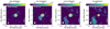 |
Fig. 1. Continuum maps of GY Aql taken with the extended (left), mid (centre left), and combined (centre right) array configurations of ALMA. The rightmost plot shows the residuals after subtracting a UD representing the AGB star (see text for details), highlighting extended dust features. The thin solid contours indicate levels of 3σ, the thick solid contours levels of 5, 10, 30, 100, and 300σ, and the dotted contours levels of −3 and −5σ. The continuum peak is indicated by the red cross, and the synthetic beam is given in the bottom-left corner of each image. The white bars on the lower right give indicative sizes in physical units for a third of the box length, based on the distance in Table 1. North is up and east to the left. |
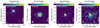 |
Fig. 4. Same as Fig. 1 but for W Aql. The position of the F9 main sequence companion is indicated by the yellow cross. |
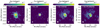 |
Fig. 7. Similar to Fig. 1 but for π1 Gru. The centre of the secondary peak, corresponding to the C companion, is marked by the black cross on the extended, combined, and UD-subtracted plots. The yellow cross in the middle-left panel indicates the position of the B companion based on Gaia observations. |
Table 1 gives an overview of the stellar properties. We describe our choice of distances and periods in the following subsections.
2.1.1. Distances
The distances given in Table 1 were collected from the literature and represent the best current estimates and uncertainties. Where available, we used the estimates and uncertainties provided by Andriantsaralaza et al. (2022), who used several methods tailored to AGB stars; otherwise, we used the results of Bailer-Jones et al. (2021) based on Gaia observations (with geometric priors). The exception is VX Sgr, for which the geometric and photo-geometric priors gave distances of 4.6 and 4.1 kpc, with uncertainties in excess of 1 kpc (Bailer-Jones et al. 2021). This is significantly larger than the value of 1.57 ± 0.27 kpc found by Chen et al. (2007) using maser proper motions. The discrepancy most likely arises from the surface variability of the star and its large angular size, which combine to make it difficult to determine the photocentre. Our adopted distance of 1570 pc is consistent with water maser proper motions (Murakawa et al. 2003) and with membership of the Sgr OB1 association (Humphreys et al. 1972). AH Sco is another RSG for which a similar maser proper motion method gives a distance of 2.26 ± 0.19 kpc (Chen & Shen 2008), in better agreement with the Bailer-Jones et al. (2021) distance of  pc. For the third RSG in our sample, KW Sgr, the Gaia distance of
  pc (Bailer-Jones et al. 2021) is in agreement with the previously estimated distance of 2.4 ± 0.3 kpc based on its membership of the Sgr OB5 association (Mel’Nik & Dambis 2009; Arroyo-Torres et al. 2013).
2.1.2. Variability
We list periods and variability types in Table 1 for all the stars in our sample. The variability types and periods were taken from the International Variable Star Index (VSX1). These periods were also further verified by cross-checking the VSX period with light curves from the American Association of Variable Star Observers (AAVSO2), All Sky Automated Survey (ASAS; Pojmanski 2002) and the ASAS-SN Variable Stars Database (Shappee et al. 2014; Jayasinghe et al. 2019) using the Lomb-Scargle periodogram (VanderPlas 2018), as the time series are unevenly sampled. Among the AGB stars we have a mix of Mira variables and semi-regular (SR) variables of types SRa and SRb. The RSGs are all SRc, as expected. The SRb stars aside from V PsA have a secondary period as well as a primary period listed in Table 1.
Key properties of the stars in our sample.
In Appendix A.1 we discuss individual stellar periods in more detail. To briefly summarise the key points, SV Aqr was reported in earlier ATOMIUM papers as a long period variable (e.g. Gottlieb et al. 2022). For the present work, we looked further into the pulsations of SV Aqr and were able to define a primary period of 93 days, as described in Appendix A.1. For π1 Gru, we identified a long secondary period (∼15 years), also described in Appendix A.1. R Aql and R Hya have been reported to have shortening periods (Wood & Zarro 1981; Greaves & Howarth 2000; Zijlstra et al. 2002; Joyce et al. 2024), possibly owing to undergoing thermal pulses in the recent past (a few hundred or so years ago). This is discussed further in Appendix A.2.
2.2. ALMA 12 m Array
Observations were taken with three configurations of the ALMA 12 m Array in Band 6 over the frequency range 214–270 GHz as part of the ATOMIUM Large Programme (2018.1.00659.L, PI: L. Decin). Typical resolutions for the extended, mid and compact array configurations are 25 mas, 200 mas, and 1″. In Table 1 we note which stars were observed with which configurations, and give a reference to which figure their continuum images are shown in (Figs. 1–17). All the compact configuration images are shown in Fig. B.1. A detailed discussion of the data reduction, including self-calibration, is given in Gottlieb et al. (2022) and a complete list of the spectral line IDs and their properties is given in Wallström et al. (2024). The maximum recoverable scales (MRSs; the scale at which smooth regions of flux can be recovered with confidence) are ∼0.4 − 0.6″ for the extended array data, 1.5″ for the mid array data, and 8 − 10″ for the compact array data. This is discussed further in Sect. 3.1, and more precise MRSs for each star and configuration are given in Table E.2 of Gottlieb et al. (2022). In this paper we focus on the continuum data, which we now analyse in detail. However, the basic parameters of the individual array continuum observations, including observation dates, are given in Table E.2 of Gottlieb et al. (2022). In Tables B.1, 3, and B.3 we give an overview of the continua observed with the extended, mid, and compact array configurations.
The ALMA 12 m array data taken in the compact configuration (lowest resolution) were observed for the shortest time spans and so have lower signal-to-noise ratios (S/N) and less positional precision. For each star and array configuration, we identified and excluded spectral lines and self-calibrated the phase-referenced continuum data, as described in Gottlieb et al. (2022). The flux scale of individual observations should be accurate to 5–7% at Band 6 (Cortes et al. 2023) and our observations met this. Where there were discrepancies due to calibration uncertainty, we rescaled an individual configuration if it was inconsistent or, if all configurations disagreed, we took the mid configuration flux densities as the most reliable standard to rescale the other configurations. This flux comparison was done for baseline lengths common between configurations and, hence, was not affected by missing spacings. The resulting flux scale is nominally accurate to ∼10%, although detailed examination (e.g. of R Hya by Homan et al. 2021) suggests that it may be better.
We fitted 2D Gaussian components to the continuum images after applying phase-reference solutions only. The accuracy of Gaussian fitting is limited by (beam size)/(S/N), where S/N is > 50 in all cases; the main astrometric uncertainty comes from transfer of calibration (Gottlieb et al. 2022). The most accurate astrometric positions (∼2 mas) were obtained for extended configuration images. The mid and compact array data were adjusted to the position of the extended array data before combination. Thus, the stellar reference positions are for the epoch June 23–July 12, 2019 (observing dates for each star are given individually in Table E1 of Gottlieb et al. 2022). Overall, data for each star was taken over a period of 6–12 months and the proper motions for each star range from 1.3–69 mas yr−1 (Gaia Collaboration 2023), likely accounting for the most significant positional shifts. The only exception is KW Sgr, for which one set of mid observations were taken in May 2021, giving a total observation range of 30 months. The proper motion shift was minimal, however, since this distant star has the smallest proper motion of our sample.
When we discuss combined data, we are referring to the ALMA 12 m array data from the extended, mid and (for most stars) compact configurations that have been combined to improve overall sensitivity while maintaining a high angular resolution. An overview of the combined data is given in Table B.4. The observed data for each separate array observation were weighted during pipeline calibration according to the integration times, channel widths, and amplitude calibration variance, but no further weighting was done in self-calibration (and flagging was done after channel averaging). The configurations were combined with equal weight. The combined MRS is generally as good as for the compact configuration data, except for AH Sco and KW Sgr, which were not observed with the compact configuration, and for which the MRS is as good as for the mid configuration data.
For any combined images with signs of artefacts such as negatives exceeding 4σ, we re-examined the data carefully. Calibration and flux scale errors are symmetric (or anti-symmetric for phase) in the stellar image, whilst angular misalignments tend to show up as anti-symmetric central adjacent errors after subtracting a uniform disc (UD; see Sect. 2.4). In a few cases we repeated the self-calibration of individual configurations with different solution intervals and other constraints to optimise the continuum. However, the main cause of artefacts was usually misalignment of the flux or position between configurations, since even within the ALMA tolerances a, for example, 5% flux scale error exceeds the dynamic range for the brighter stars. We therefore aligned the configurations to minimise the relative errors.
2.3. ALMA Compact Array
A subset of the ATOMIUM sample was also observed in Band 3 with the Morita Array (ALMA Compact Array; project 2019.1.00187.S, PI: T. Danilovich). The observations were taken over discrete spectral windows in the frequency range 97–113 GHz. The central frequency for the continuum images is 104.96 GHz. The MRSs for these observations fall in the range 64–77″. The flux scale accuracy of these data is around 5% (Cortes et al. 2023). Note that we refer to observations with the Morita Array as ‘ACA data’ and to observations with the compact configuration of the ALMA 12 m Array as ‘compact data’. The details of the ACA data are given in Table B.5. In Fig. B.2 we show all the continuum images obtained using the ACA.
All the ACA data used comes from the standard ALMA pipeline (and has not been self-calibrated) aside from RW Sco, for which we created a custom dataset that was not primary beam corrected. The reason for this is a confounding nearby source, approximately 27″ south of RW Sco, which is intrinsically brighter than the AGB star once the primary beam correction is applied. This is discussed further in Appendix C. We present some line observations obtained concurrently with the ACA continuum in Appendix D.
2.4. Fitting uniform discs
For the Band 6 observations of each star, we show the amplitudes of the visibilities as a function of uv distance in Fig. B.3. These plots generally indicate a compact component and, in many cases, some extended features; the latter is discussed in more detail in Sect. 3. At radio frequencies, for example centimetre to sub-millimetre wavelengths, the main compact contribution to the continuum emission is expected to come from electron-neutral free-free emission in an extended radio photosphere, above the stellar photosphere (Reid & Menten 1997; Matthews et al. 2015; Vlemmings et al. 2019). Emission offset from the stellar position, assumed to be the continuum peak, most likely originates from dust surrounding the stellar photosphere and radiosphere (see Sect. 3).
To estimate the stellar sizes and flux densities, we fitted a UD model to the calibrated, line-free combined Band 6 visibilities for each source. We tested Gaussian fits but found higher residuals, indicating worse fits. Trying to fit a UD + a point source at the stellar position also gave worse results, including relatively bright residuals within the stellar disc diameter. This suggests that any stellar-related flux not fit by a UD is not concentrated in a single point and is not symmetric, i.e. has a random or more complex and blotchy distribution, which cannot be fit in the uv plane. We also found that the irregularities in the sources are greater than any differences between a UD or a limb-darkened disc (where a limb-darkened disc is similar to what Bojnordi Arbab et al. 2024 found from their models).
For the UD fits we used the Common Astronomy Software Applications (CASA, The CASA Team et al. 2022) task uvmodelfit to fit a single UD to the data. In the case of AH Sco, RW Sco, and π1 Gru, we used the uvmultifit package (Martí-Vidal et al. 2014), which has many capabilities, including the ability to fit multiple components and more detailed constraints at low S/N, which allowed us to ensure that the diameter and flux did not simply match pre-set limits. For our sample of evolved stars, we report only single component fits as adding more components, whether points or extended emission, did not converge to a stable solution, suggesting that any star-spots and/or extended dust cannot be described by simple, symmetric components. For AH Sco and IRC+10011, we used the extended configuration data only as there are irregularities on short spacings. These are probably due to large-scale flux that is irregularly or asymmetrically distributed, possibly simply contributing a small excess on short baselines but smooth enough on large scales to be resolved out for long baselines. For most stars such irregularities did not affect the fit, but for AH Sco (because of low S/N) and IRC+10011 (significant resolved-out flux; see Sect. 3.1), the errors in the fit were much greater if short baselines were included. For RW Sco we forced the position to be at the phase centre, as it has very weak continuum. In each case, the starting model was the literature optical diameter and peak flux density from Tables 1 and E.2 in Gottlieb et al. (2022). All parameters (peak, position, diameter, ellipticity, position angle) were allowed to vary except for the special case of π1 Gru, for which a close companion (π1 Gru C, separation ∼0.038″) was reported by Homan et al. (2021). Hence, for π1 Gru we first subtracted the companion and then fixed the position and ellipticity (none) to avoid contamination by the companion residuals. This two-component fit was done using only the extended array data, but we find the UD model agrees with the full dataset, except at the shortest baselines (see Fig. B.3). π1 Gru C is too faint and compact to be resolved even by component fitting so we do not give its size (see Fig. 7, in which it is comparable to the extended data beam size). We determine an integrated flux density for π1 Gru C of 2.78 mJy.
For SV Aqr, attempts to fit to the visibilities for all configurations failed to resolve the star and could only measure the flux density within the central 15 mas with any confidence. The result of this fit is shown in Fig. B.3. However, to retrieve more reliable stellar parameters, we performed a fit in the image plane using the extended configuration data only, which retrieved the parameters with S/N > 5. It is these parameters that are included in Table 2.
Results of the UD fits.
The fitting routines report the uncertainties in the fits. The disc fits were almost circular (r = minor/major axis ratio > 0.9) for most sources, except RW Sco and KW Sgr (which have low S/N) and IRC−10529 (r = 0.87), and U Her (r = 0.89), for which the diameter listed in Table 2 is the longer axis. We assumed that the stars are unlikely to be elliptical to this degree, but instead that deviations are due to either elliptical beams (Table B.4) or stellar surface irregularities probably distributed randomly. We thus took the ellipticity as a contribution to the uncertainty in the fit. The other contributions are the observational errors. Phase errors contribute a size uncertainty proportional to the (beam size)/(S/N), and the flux density errors are mostly dominated by the flux scale uncertainty except for the weakest sources where the noise is significant (see Gottlieb et al. 2022).
The resulting UD parameters are given in Table 2 and the visibility amplitudes with the fitted UD models are shown in Fig. B.3. The error bars on the visibilities represent the observational scatter of the visibility amplitudes in each bin. The shaded regions represent the fitting errors with the edges of the shaded region representing the upper and lower extremes of these uncertainties. The rms values given in Table 2 do not represent the total uncertainty on the flux and should be added in quadrature with a 10% calibration uncertainty on the flux, though in some cases this uncertainty appears to be much better (based on consistency between observations with different calibrators).
We were unable to find good fits for KW Sgr or RW Sco because these two sources have low S/N and small angular sizes, consistent with being unresolved. (Note that the other stars, aside from SV Aqr, have S/N > 50.) We still list the best fitting parameters for these stars in Table 2 and show the fits in Fig. B.3 but note the very large uncertainties on the UD diameters. In Table 1, we give the right ascension and declination (in the International Celestial Reference System, ICRS) determined from the UD fits, which in all cases are within 1 mas of the astrometric positions (see Sect. 2.2 and Gottlieb et al. 2022). Preliminary UD sizes were reported for 5 of the ATOMIUM sources previously (R Aql, U Her, R Hya, T Mic, and S Pav; Baudry et al. 2023, see also Homan et al. 2021 for R Hya). Those sizes were within 1% of what we find in the present work, except for R Hya where the size difference is ∼10%. The improvement in the R Hya fit comes from the adjustments to the relative positions and fluxes described in Sect. 2.2, which enabled us to improve the dynamic range from ∼1500 to 6500.
Based on our UD fits we also calculated brightness temperatures for our sample, using 241.75 GHz as the central frequency of our combined data. An explanation of this calculation is given in Appendix E. The resultant brightness temperatures are given in Table 2, excluding RW Sco, for which the UD fit values were too uncertain to implement. The uncertainties we find for KW Sgr and SV Aqr are very large, but we list the obtained values in the table for completion. The flux densities of these sources are the lowest in our sample. Note that KW Sgr is our most distant target. For the sample overall, the derived brightness temperatures are in the range 760–2300 K, all systematically cooler than the effective stellar temperatures collected from the literature (see Table 5), but many are largely in line with the earlier results of Vlemmings et al. (2019), for four nearby AGB stars. The theoretical predictions of Bojnordi Arbab et al. (2024) give phase-dependent brightness temperatures ≳1900 K, depending on the model. Where our brightness temperatures are notably lower than this, we assume it is because newly formed dust, located close to the surface of the star, has been captured by our best-fitting UD.
We subtracted the UD models from the combined visibility data and imaged the residuals, which we show alongside the continuum images in Figs. 1–17. We weighted the baselines during imaging (see Sect. 3) to provide a larger synthesised beam than was used for the un-subtracted combined images, to give better sensitivity to features with low surface brightness. The exceptions are GY Aql and π1 Gru, for which we used a synthesised beam of comparable size to the combined image in order to resolve the faint, but compact and distinct, offset emission. The details of the UD-subtracted images are given in Table B.6. For SV Aqr we show the residual image after subtracting the original UD fit to the combined data (Fig. 5), which represents contributions from the star and possibly some inner dust. We caution that the resulting features are not as reliable as for the other stars and should not be over-interpreted.
3. Continuum imaging
The combined visibility data provide sensitivity to emission on scales from a few tens of mas up to 8–10″. However, the visibility plane coverage is not complete nor evenly distributed. To avoid artefacts due to missing spacings between the longest baselines, we applied a slight taper in imaging to weight down their contribution, providing resolutions ∼50 mas. Residual calibration errors and antenna position errors limit the dynamic range3 to about 1000, so for the brightest stars, for example R Hya (Fig. 9), symmetric negative and positive artefacts may be present at < 0.1% of the peak. Tables B.1, 3, B.3, and B.4 include the dynamic ranges for for the extended, mid, compact and combined data, respectively. The ACA continua have relatively low dynamic ranges, from 4 for RW Sco to 50 for T Mic (Table B.5 and Fig. B.2).
Smooth emission on scales much greater than 10″ will not be detected, but any extended dust on around this scale can cause bowl-like artefacts due to being detected by just a few baselines. Artefacts can also arise from intermediate under-sampled scales. In general, for the brightest stars, if there are regions of negative flux (indicated by dotted contours at the 3 and 5σ levels), corresponding positive regions at those levels or weaker should be treated with caution. The noise rms given in Table 2, used to estimate the accuracy of quantities derived from UD fits, are measured close to the stellar position. The background noise far from the star is given in Tables B.1–B.4 for the extended, mid, compact and combined array data, respectively. The combined noise at > 1″ is ≲0.01 mJy.
The continuum images for the extended, mid and combined data are plotted, per star, in Figs. 1–17, as indicated for each star in Table 1. We also include in these figures combined images of the residuals after subtracting UDs representing the AGB stars and sometimes including dust close to the stars (as described in Sect. 2.4). The compact array data are plotted for all observed stars in Fig. B.1 and the Band 3 ACA data are shown in Fig. B.2. In general, the compact configuration images are unresolved or marginally resolved, with some stars exhibiting small (≲ beam) irregular extended regions of flux detected at the 3σ level. We can determine that the bulk of the flux is unresolved because it mimics the elliptical shape of the beam down to the 5 or 10σ level. All of the ACA images are unresolved, owing to the large beams (see Table B.5).
In the following subsection we discuss the issue of resolved out flux. Subsequently we discuss the unresolved continuum emission, then some stars grouped by similar continuum features and some stars individually when they exhibit relatively unique features. These groupings are summarised in Table 3.
Overview of the morphological classification of the continuum images.
3.1. Resolved-out flux
As noted in Sect. 2.2, ALMA is not guaranteed to recover all the flux associated with a source and may resolve out some smooth large-scale flux. We were able to check the impact of this effect for four ATOMIUM stars that are also in the DEtermining Accurate mass-loss rates of THermally pulsing AGB STARs survey (DEATHSTAR, Ramstedt et al. 2020). DEATHSTAR observed a large sample of AGB stars using the ALMA ACA in Bands 6 and 7. For their Band 6 observations – which cover similar frequencies as ATOMIUM, albeit over a smaller range – the MRS was 25 ± 4″ (Ramstedt et al. 2020). We compared the self-calibrated Band 6 continuum fluxes from DEATHSTAR with those from our ATOMIUM combined and compact continuum images, for the overlapping stars (IRC−10529, SV Aqr, T Mic, and IRC+10011). We found no evidence of more flux being resolved out for the ATOMIUM data than for the DEATHSTAR data.
However, this does not mean that all the flux has necessarily been recovered. Herschel/PACS images of dust at 70 and 160 μm are available for some of the stars in our sample. For W Aql, π1 Gru, R Hya, and T Mic, extended flux is seen on scales of ∼1′ from the position of the star, indicating significant dust at larger scales than can be recovered with ALMA (Cox et al. 2012). This is significant because at longer wavelengths (i.e. 1.2–1.3 mm for ALMA Band 6) we might detect cooler dust, which we would expect to be located further from the star. However, since ALMA cannot recover flux on such large scales – scales that can be larger than the ALMA field of view for a single pointing – we would not expect the majority of flux from such a large dust shell to be recovered, even when using the ACA. Comparing our total combined fluxes (Table B.4) with single-dish observations from Altenhoff et al. (1994) and Dehaes et al. (2007), we can estimate the recovered fluxes for R Aql, R Hya, and IRC+10011 as around 60%, 70%, and 6–12%, respectively. The large amount of resolved out flux for IRC+10011 (88–94% lost) fits with the negative artefacts we see in Fig. 12.
To give an indication of what fraction of flux comes from regions offset from the continuum peak, we compared the UD flux density (see Table 2 and Sect. 2.4) with the total flux recovered in our combined images (Table B.4). Overall, we find no significant correlation with distance to the stars. Excluding the RSGs, we find a weak positive correlation between the flux ratio and distance, which is expected, since a more distant source will appear smaller on the sky and hence be less susceptible to resolved-out flux. Also, for the closest sources, the full extent of the circumstellar envelope may be larger than the primary beam of the ALMA 12-m array. Across our sample, there is a large spread in the ratios of total flux to UD flux, from 1.07 (U Del) to 2.24 (IRC−10529). U Del having the lowest flux ratio fits with what we found from the UD-subtracted map (Fig. 6), which shows that the majority of the continuum flux is associated with a UD of emission at the stellar position and that there is essentially no extended flux recovered by ALMA. The stars with the highest ratio (IRC−10529 followed by W Aql) exhibit flux away from the continuum peak. Some of the other stars with lower flux ratios nevertheless have extended features, likely arising from dust, in their continuum maps, or are known to be dusty based on other observations (e.g. Herschel/PACS imaging; Cox et al. 2012; Maercker et al. 2022). This discrepancy could be caused by resolved-out flux, amplitude errors (especially for sources with high dynamic ranges > 1000) or a combination of factors.
We also checked whether there was any correlation between the ratio of total flux and UD flux density with the apparent or physical UD radii and found no trends. We find no correlation between the total flux or UD flux with mass-loss rate, distance, or mass-loss rate scaled by distance.
In summary, it is likely that there is resolved out flux for at least some of our observed stars. The precise fraction of recovered flux is difficult to estimate from the available data, for the majority of our sample. The stars that are further away or which have smaller dust extents are less likely to be affected.
3.2. Resolution-limited continuum images
In general, we expect spatially resolved emission to appear larger than the restoring beam of the observing array. For emission with spatial extents much larger than the beam, this is trivially apparent (see for example the ATOMIUM CO emission, Decin et al. 2020). However, a bright point-like source with a high dynamic range can appear to be larger in the image plane than the reported beam size, because of the Gaussian nature of the beam. This is explained in detail in Appendix F, where we lay out criteria for checking whether bright sources show evidence of resolved emission. Note that fitting in the visibility plane, as we did for the UD fits (Sect. 2.4), avoids apparent extension due to convolution with the beam, but is still S/N-limited.
The most sensitive continuum images, capable of revealing the most extreme small- and large-scale features, were made from the combined data. Most of our sources exhibit some extended emission in the combined maps, though in some cases, such as KW Sgr (Fig. 15), the extended emission is not apparent until we subtract a UD from the data and lower the resolution to increase sensitivity (Sect. 2.4). For the particular example of KW Sgr, this is discussed further in Sect. 5.1.6. Two stars, U Del (Fig. 6) and RW Sco (Fig. 14), do not show any extended emission in the combined maps or the UD-subtracted maps. U Del is so well described by the UD that there is no significant flux in the UD-subtracted map at all. T Mic (Fig. 10) and V PsA (Fig. 13) appear unresolved in the combined maps, but the UD-subtracted maps reveal some small (comparable to the beam) regions of emission offset from the continuum peaks. The combined continuum maps for the remaining stars all show more significant extended emission and/or asymmetries, which are described in the following subsections.
When considering the individual array images in the context of our criteria for resolution, we find that almost all of our compact images (Fig. B.1) are close to the resolution criterion defined in Appendix F, i.e. within 10% at the 5σ level, with only a few stars such as W Aql and S Pav showing evidence of extended emission ≥20% of the resolution criterion. For observations with the mid configuration, a larger portion of the images show evidence of (partially) resolved extended emission. Some cases of faint extended emission seem to be below the sensitivity limit of the mid data, but above 3σ in the combined data, making sources such as S Pav (Fig. 11) appear unresolved in the mid images. Most images taken with the extended array show evidence of resolved out flux to varying degrees, with only a few stars for which clumpy extended emission is recovered. A prime example of this is π1 Gru (Fig. 7), which we discuss in detail in Sect. 3.5.5.
3.3. Stars with relatively uniform extended flux
Based on the criteria laid out in Appendix F, the majority of the stars in our sample have some extended continuum emission associated with them. Of these, relatively uniform extended flux is seen in the combined and UD-subtracted continuum images of U Her (Fig. 8), R Hya (Fig. 9), S Pav (Fig. 11), and IRC+10011 (Fig. 12). In these cases, the flux is relatively symmetric about the stellar positions, though not perfectly so. U Her and R Hya also exhibit some extended emission in their mid continuum maps.
3.3.1. U Her
The continuum maps of U Her in Fig. 8 show significant extended emission surrounding the continuum peak, most clearly apparent in the UD-subtracted image, where the regions of extended emission much larger than the beam. The mid and extended maps show asymmetric features at the 5σ level.
In the combined map, the larger-scale emission at ≥3σ extends to separations of around 0.4″ to the south, west, and north, but only out to ∼0.2″ to the ENE. The emission is not distributed evenly and is clumpier to the N and NW. In the extended, mid and combined maps, there is a small region (at different scales for each map) with less emission to the south of the continuum peak. The cause of this region of lower emission is unclear, but the fact that we see it at all scales suggests that either a continuous or repeating process is causing it.
3.3.2. R Hya
The continuum observations of R Hya (Fig. 9) have the highest dynamic range of any star in our sample, exceeding 1000 for all individual array configurations, and reaching 6600 for the combined data (see Tables B.1–B.4). This may be partly due to the fact that R Hya is the closest star in our sample (distance = 126 pc). The roughly symmetric negative regions surrounding the continuum peak in the extended and combined maps shown in Fig. 9 are the result of amplitude errors. However, the UD-subtracted map shows significant extended flux at levels of ≥5σ out to 0.15–0.3″ from the stellar position.
The mid continuum map has scattered regions of emission around the central continuum peak. These include emission detected with a certainty of 5σ extended out to ∼0.75″.
Finally, we note that a combined continuum map of R Hya was previously published by Homan et al. (2021) and showed a highly asymmetric structure in the inner regions, positive to the E and negative to the WNW. In carefully re-imaging the data, we discovered that these features resulted from a misalignment of the mid array data and did not represent real features. Although some minor artefacts remain in our extended and combined images, they are a more accurate representation of the dust distribution around R Hya.
3.3.3. S Pav
The S Pav extended and mid continuum images (Fig. 11) are relatively featureless, but the compact map shows some asymmetric protrusions to the NW and SE (Fig. B.1). The combined map and the UD-subtracted map show significant extended flux, with the 3σ contour located at around 0.2″ from the continuum peak. This corresponds to a physical projected separation of 37 au from the continuum peak. No clear structures are resolved in this extended emission in the UD-subtracted image. Even when we consider the un-subtracted combined image with a smaller synthetic beam, no obvious structures become apparent and all irregular regions are of comparable in size to the beam or smaller, making it difficult to discern their actual sizes.
3.3.4. IRC+10011 (WX Psc)
Examining the continuum maps for IRC+10011 in Fig. 12, we find that the mid map has two small protrusions at 3σ that are smaller in width than the beam and are approximately rotationally symmetric. There are also protrusions in the extended map to the SE and NE, at a level of 5σ and to the NW at a level of 3σ, which are not very symmetric. Similar features, at larger scales, can be seen in the combined map. However, the combined map shows more symmetric features and some regions of negative flux surrounding the continuum peak. These are most likely the result of phase and/or amplitude errors.
The UD-subtracted map should not suffer from sidelobe or dynamic range artefacts since the stellar contribution has been subtracted. We find that the flux is roughly evenly distributed around the continuum peak, with extensions to the north and south. The shape of the 3 and 5σ contours enclosing the UD-subtracted flux corresponds well with the central part of the combined map, excluding possible artefacts to the east and west.
3.4. Elongated continuum features
Identifying elongated structures in the continuum maps can be challenging, as any symmetric features (of positive or negative flux) may be the result of amplitude errors. These are more likely to be present for higher dynamic ranges. Since our sample contains many bright sources, we must be careful when interpreting any symmetric elongated features. With this in mind, we have tentatively identified a group of stars that exhibit some elongated features. These are IRC−10529 (Fig. 3), T Mic (Fig. 10), and VX Sgr (Fig. 16).
3.4.1. IRC−10529 (V1300 Aql)
The extended map of IRC−10529 (Fig. 3) features some small symmetric protrusions to the NW and SE, which may be amplitude errors rather than real features. However, there is a small region of extended flux to the SW, in the extended and mid maps, which is likely real and is not mirrored on the other side. The combined map shows an elongated emission structure, with some emission extending from the continuum peak to the WSW and ENE. This elongated structure, which runs along an axis ∼70° east from north, is detected with more confidence in the UD-subtracted map, which emphasises lower surface brightness features thanks to its lower angular resolution. This axis is comparable to the axis about which the positive and negative velocities are separated in the SiO moment 1 map shown in Fig. S60 of Decin et al. (2020). There are also some perpendicular extensions that are not symmetric about the location of the continuum peak, and which are somewhat reminiscent of the shape to the Red Rectangle protoplanetary nebula (Cohen et al. 2004), but on a much smaller scale.
3.4.2. T Mic
Although the individual array images of T Mic (Fig. 10) are unresolved, the UD-subtracted image reveals a region to the NW at a significance of 3 − 5σ and a more elongated region, at around 3σ, to the SE. The coarser beam size of the UD-subtracted image increases the signal to noise of features that are not confidently detected in the combined map with a smaller restoring beam. Drawing a line between the continuum peak and the northern feature in the UD map, we find that it lies approximately 25° west of north. This is in the same direction as the brightest feature seen in polarised light by Montargès et al. (2023) using the Spectro-Polarimetric High-contrast Exoplanet REsearch on the Very Large Telescope (VLT/SPHERE), as we plot in Fig. 18, raising confidence that this elongated structure is real. The angle of this feature is approximately perpendicular to the angle separating positive and negative velocities in the 30SiO (J = 6 → 5) moment 1 map presented in Decin et al. (2020).
 |
Fig. 18. DoLP around T Mic observed with SPHERE (from Montargès et al. 2023) with the UD-subtracted contours observed with ALMA plotted in white (see Fig. 10). The position of the AGB star is indicated by the green cross. |
3.4.3. VX Sgr
Some asymmetric features are seen for all the continuum maps of VX Sgr (Fig. 16). These are most pronounced for the extended and combined maps, where emission is seen predominantly to the south and north of the continuum peak. Once again, this emission is most pronounced in the UD-subtracted map. Considering only the emission closest to the location of the continuum peak (e.g. the emission enclosed by the 5σ contour), we find that the elongation axis is close to running due north-south, with an uncertainty of only a few degrees (< 5°). We note that this emission could be the result of episodic mass loss, as discussed in Sect. 5.1.7.
3.5. Highly asymmetric continuum features
Some of the stars in our sample exhibit features in their continuum maps that are neither uniformly extended nor bipolar. Generally, the resultant maps are unique, so we discuss these stars individually below.
3.5.1. GY Aql
GY Aql is unusual in that the continuum maps from the extended and compact array configurations show unresolved emission (Figs. 1, B.1), but a strongly detected feature is seen to the SE in the mid and combined maps. In the mid map, this feature appears attached to the continuum peak and is detected at a level > 30σ. When constructing the combined image, we found that choosing a restoring beam that was too fine would result in this feature having a very low surface brightness and not being detected above the noise, beyond a small region with the brightest flux (visible at an offset of 0.5, −0.5 in Fig. 1). Hence, we chose a coarser resolution for the combined map than was used for most other stars (see Table B.4) to emphasise this feature, which appears detached and which we refer to as a ‘bar’, though it may be part of a spiral, since spiral-like structures are seen in the CO emission (Decin et al. 2020). As can be seen in the UD-subtracted map, the continuum flux mainly originates from this bar and from regions close to the star, likely indicating a significant concentration of dust in this bar.
3.5.2. R Aql
In constructing the combined continuum image, we found suspiciously regular positive and negative patches of emission, larger than the synthesised beam, at levels of ≳3σ around the continuum peak. This suggests resolved-out emission. Tapering to give more weight to shorter baselines, i.e. coarsening the resolution, alleviated some of this effect and allowed us to recover more flux and structures in the combined map, which is shown in Fig. 2. The extended continuum emission is patchy and irregularly distributed around the continuum peak. Hints of these structures can also be seen in the marginally resolved mid continuum map. The extended continuum map of R Aql has a very high dynamic range, in excess of 2000, resulting in increased uncertainty; as such, features in the map at < 0.1% of the peak should be treated with caution, especially if they are symmetric. All the larger scale structures visible in the mid and combined maps are resolved-out in the extended map.
3.5.3. W Aql
W Aql has a known main sequence (F9) companion at a projected separation of ∼0.5″, corresponding to a physical separation ≈200 au (Danilovich et al. 2015a, 2024). The individual higher-resolution 12 m array continuum images, plotted in Fig. 4, show a secondary peak, detected with a certainty of 5σ, to the SW of the primary continuum peak. Taking the primary peak as the position of the AGB star, the secondary peak corresponds well to the location of the F9 companion, which was observed with VLT/SPHERE contemporaneously with the extended array data (July 9, 2019; Montargès et al. 2023, a day after the ALMA observations were completed). We indicate the position of the companion as observed with SPHERE by the yellow cross in Fig. 4. While some extended emission is resolved around the primary peak with the extended array, the secondary peak appears as a point source in the extended and combined continuum maps. It is only marginally resolved from the primary peak in the mid continuum and not at all in the compact continuum (Fig. B.1). At this wavelength (1.24 mm), the F9 companion is well below the detection threshold, so this significant detection indicates a concentration of dust close to the F9 star, the origin of which is discussed in more detail in Sect. 5.1.2.
There is some additional extended continuum emission surrounding the primary peak, especially to the E and NE. In the mid and compact (Fig. B.1) continuum maps there is some emission extending further than what is visible in the extended and combined maps, suggesting that some larger scale flux may be resolved out at those higher resolutions. The UD-subtracted image also shows areas of extended emission towards the south and west, though the surface brightness is lower and it is only detected at levels of ∼3σ. The peak flux in the UD-subtracted image is very slightly offset from the continuum peak but indicates substantial emission close to the AGB star.
3.5.4. SV Aqr
As can be seen in Fig. 5, there are some small regions of extended flux around the continuum peak of SV Aqr. In the extended map, there are some protrusions to the W and SSW of the continuum peak, and some smaller regions scattered at larger distances (∼0.2″) from the continuum peak. In the mid image, there is a small protrusion to the NW. The combined map shows an elongation in the W and SSW directions, in similar positions to the protrusions seen in the extended map, and some scattered emission to the NW, aligned with the direction of the protrusion in the mid map. Hence, the combined map represents the emission at both larger and smaller scales well.
The peak flux in the UD-subtracted image is to the SW and not centred on the continuum peak in the un-subtracted image. The UD subtraction reveals an arc of emission close to the stellar position in the S and SE, which appears to sweep anti-clockwise to the NW, where it is located further from the star (the 3σ contour extends out to 0.12″). This strongly asymmetric feature likely contributed to our difficulty in fitting a UD to SV Aqr (see Sect. 2.4) and we stress that the features presented in the UD-subtracted image are not reliable, aside from where they agree with the individual array images.
3.5.5. π1 Gru
Homan et al. (2020) previously presented the extended continuum map of π1 Gru, which shows a close secondary peak to the SW of the primary continuum peak. Here we present the continuum maps obtained from the other ALMA arrays and the combined continuum map for the first time (Figs. 7 and B.1). We also present the ACA Band 3 continuum map (Fig. B.2).
The secondary peak is marked by a black cross on the extended and combined continuum plots in Fig. 7. We henceforth refer to this feature as the C companion, following Montargès et al. (2025). The AGB star, which we associate with the position of the primary continuum peak, is the A component and the B component is a long-known main sequence G0V star (Feast 1953), which, in the Gaia DR3 epoch (2016.0), is separated from the AGB star by 2.68″ (Gaia Collaboration 2021), corresponding to a projected separation of 440 au. The B component is outside of the plotted field of views of the extended and combined data, but we indicate its approximate relative position (calculated from the Gaia catalogue by assuming that the separation between A and B did not significantly change between the Gaia epoch and our ALMA observations) as a yellow cross on the plot of the mid continuum image (Fig. 7) and the compact continuum image in Fig. B.1. We do not detect any emission above the noise near the position of the B companion, in contrast with W Aql, which may be because the companion is more distant and situated in a less dense wind (e.g. compare the mass-loss rates in Table G.1).
The C component is visible as a secondary peak in the extended continuum map, but is not resolved in the combined map. Instead, the combined map shows a central feature elongated in the direction of the C component. There is also some additional extended emission seen around the central peak in all directions except for the SW. This ‘tail’ of extended emission corresponds well with the tail seen in the contemporaneously observed VLT/SPHERE image showing the DoLP presented by Montargès et al. (2023) and is discussed further in Sect. 5.1.1. There is also some scattered emission present in all directions around the continuum peak in the mid image with, as noted above, a slight bias in the direction of the B component.
For the UD-subtracted image shown in Fig. 7, we chose a comparable synthetic beam to the combined image to better emphasise the tail of emission. Once the flux from the AGB star is subtracted from the continuum map, the peak flux is found at the position of the C component and has the highest relative flux (i.e. the highest dynamic range; see Table B.6) of any UD-subtracted image in our sample, by a factor of ∼5 or higher. For finer resolutions of the UD-subtracted image, we find that the low surface brightness of the tail feature caused it to be lost in the noise. At coarser resolutions, the tail is not necessarily resolved from the dust close to the A and C components. Additionally subtracting a point-like function representing the C component does not reveal other structures.
3.5.6. AH Sco
The extended continuum map of AH Sco, shown in Fig. 17, is relatively featureless, with only a few asymmetric features, smaller than the beam, surrounding the continuum peak. The mid image, in contrast, exhibits significant extended flux around the continuum peak, similar to the combined map of S Pav (Fig. 11). There generally appears to be more extended flux to the NE and to the SW. Our understanding of this source is complicated, however, by the reverse-N shaped (or perhaps barred spiral) emission pattern seen in the combined and UD-subtracted maps. It is unclear whether the gaps in emission to the NE and SW of the continuum peak are real, for example representing a dust shell, or whether they originate from amplitude errors.
The most extended features in the continuum around AH Sco lie close to the NE-SW axis (45 − 50°). There is a feature resembling a bar perpendicular to this axis and in which there do not appear to be gaps in the flux. The most extended 3σ contours lie at 0.3″ for the first feature and at 0.25″ for the bar-like feature. These values correspond to projected separations of 520 and 430 au.
4. Analysis
4.1. Spectral indices
4.1.1. Intra-Band 6 spectral indices
Since our Band 6 observations covered frequencies spanning ∼56 GHz, we were able to calculate intra-Band 6 spectral indices for our sample. In cleaning an image with tclean, as well as identifying the brightest pixels in each cycle, we used the option to fit for the linear dependence of flux with frequency, using the first two terms of a Taylor series, giving total intensity and spectral index (alpha) images. We use the alpha.error image produced by tclean to exclude unreliable spectral index measurements, but for a well-cleaned image, this is a lower limit to the actual error, since it is based only on the residual noise in the zeroth and first Taylor coefficient images. This does not include systematic errors such as in alignment or calibration (indeed, a well-known diagnostic for tiny spatial misalignments is a systematic gradient in alpha across an image).
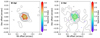 |
Fig. 19. Examples of spectral index determinations for W Aql (left) and U Her (right) computed from the combined Band 6 data. The spectral index (colours) is shown for the pixels where it is well-defined. The dashed green circle indicates the area, centred on the continuum peak, equal to the beam size convolved with the UD radius. Black contours indicate the combined continuum (see Figs. 4 and 8). Similar plots for the remaining ATOMIUM sources are given in Fig. B.5. |
Without additional calibrators or dedicated flux scale measurements, the accuracy of an individual ALMA observation at Band 6 is 5% at best. Each mid and extended configuration dataset contains at least four observations at four sets of frequencies (see Fig. 1 of Gottlieb et al. 2022 for the ranges covered in each tuning). Our calibration methods force the spectral index to be linear, but if both sets of the lowest and the highest frequencies have 5% errors in the opposite sense, this could tilt the spectral index by about 0.3, regardless of S/N. Statistically, this is likely to affect one or two out of our 17 datasets, per configuration. Another factor is the potential presence of residual lines. The combined or extended configuration data possess the most baselines sampling the smallest angular scales, meaning that these can be used for measuring the spectral index of the stellar continuum. The S/N of any other continuum features (e.g. any extended emission) is much too low for a reliable spectral index measurement.
We find that for most stars, the uncertainty on the spectral index becomes very high further than ∼1 beam from the continuum peak. Hence, to compute average spectral indices, αB6, we only consider pixels (i) that are within the circular region corresponding to the major axis of the beam convolved with the size of the UD fit to the star and (ii) for which the uncertainty on the spectral index is < 0.1. Then, for these selected pixels, we construct a histogram of the spectral indices and derive a Gaussian kernel density estimation (KDE). The peak of this KDE is taken to be the spectral index. The uncertainty is then conservatively taken to be the sum in quadrature of the full width at half maximum of the KDE and the maximum uncertainty on the individual pixels. To check the robustness of this estimate, we also considered the spectral index of the pixel closest to the continuum peak and the mean spectral index of all the selected pixels. The results of both methods agree well with our final value.
Our calculated αB6 are give in Table 4. Example plots of the spectral index for W Aql and U Her are given in Fig. 19. The remaining stars are shown in Fig. B.5 and the KDEs of the spectral indices are shown for all stars in Fig. B.6. We were unable to extract a value of αB6 for RW Sco from the combined data because the low S/N resulted in very large uncertainties on the spectral index. However, using only the extended array data we were able to estimate a spectral index for RW Sco.
Spectral indices calculated from our observations.
For π1 Gru we get an anomalously high αB6 ≳ 3. This is higher than the Band 6 to Band 7 value, αB6 − B7 = 1.9 ± 0.3, found by Esseldeurs et al. (2025), and the Band 3 to Band 6 value we find, αB3 − B6 = 1.8 ± 0.4, details in Sect. 4.1.2. The Band 6 mid data gave a value closer to the multi-band measurements. We suspect that the extended data for this star was affected by all the possible sources of uncertainty mentioned above and thus acts as a caution in using in-band spectral indices.
4.1.2. Band 3 to Band 6 spectral indices
For the seven stars in our ACA Band 3 sample we also calculate band-to-band spectral indices, αB3 − B6. Because all the stars are unresolved in the large (10–15″) synthesised beams of the ACA data, we use the peak fluxes to approximate the total flux. We also fit 2D Gaussians to the observations to extract the integrated flux and found equivalent values, within the uncertainties. The peak fluxes are listed in Table B.5. We adopt 104.96 GHz as the central frequency of the Band 3 ACA continua and 238.45 GHz as the central frequency of the Main Array Band 6 compact configuration continua4. The spectral indices are then calculated from these values and the peak fluxes of the ACA and compact data (Table B.3). The resultant spectral indices are listed in Table 4 and fall in the range 1.7–2.5, aside from RW Sco, for which αB3 − B6 = 1.0 ± 0.2. This is most likely the result of the low S/N measurements for this star.
4.1.3. Trends with spectral index
Within our uncertainties (aside from RW Sco and π1 Gru), the αB6 and αB3 − B6 spectral indices agree with each other. Aside from the outliers already discussed, we find that the spectral indices for all our stars ∼2. This agrees with the theoretical predictions for unresolved spectral indices calculated by Bojnordi Arbab et al. (2024). Since we were only able to reliably derive the αB6 spectral indices close to the star (essentially only at the continuum peak), we would expect the main contribution to the spectral index to come from the star itself. This is borne out by the predictions of Bojnordi Arbab et al. (2024); although they find variations in the unresolved spectral index with pulsation phase, their values are in the range ∼1.7–2.05 over frequencies from 100–300 GHz, in good agreement with our results. It is likely that the αB3 − B6 values are also dominated by the stars since, for the same enclosed regions, the flux densities of the standard combined maps (Table B.4) are a factor of 2–10 higher than the flux densities of the UD-subtracted maps (Table B.6). In general, the value of ∼2 of the spectral index is consistent with optically thick blackbody emission, another indication that the stellar contribution dominates.
We checked the data for possible correlations between the spectral index and other parameters, searching for trends or systematics. We find no significant correlation between spectral index and distance, suggesting that there is no factor uniformly affecting only the closest or most distant stars. For αB3 − B6 we checked for correlations between the spectral index and the individual ACA or 12-m fluxes and found none. We also found no apparent correlation between spectral index and stellar pulsation period. There is a tentative positive correlation between αB6 and the mass-loss rate (see Appendix G for details on the mass-loss rates), with low statistical significance. The models of Bojnordi Arbab et al. (2024) predict a slightly larger spread in unresolved spectral indices for their higher mass-loss rate model (2 × 10⁻⁶ M⊙ yr−1 compared with their canonical 3 × 10⁻⁷ M⊙ yr−1 model), but only to 1.55–2.1 in the 100–300 GHz range. We hence suggest that this tentative correlation between spectral index and mass-loss rate requires further observations to confirm.
4.2. Dust mass estimates
Having calculated the spectral indices for our sample, we can now estimate the mass of the dust visible in our ALMA observations. Following Knapp et al. (1993) we estimate the dust masses using
 (1)
(1)
where FUDsub is the total flux density of the UD-subtracted continuum image, ag is the radius of the dust grains, assumed to be spherical, which we take as 0.3 μm, ρg is the mass density of the dust grains, which we take as 3.3 g cm−3, c is the speed of light, d is the distance to the star (see Table 1), ν is the frequency, here 241.75 GHz, Qν is the grain emissivity at ν, kB is the Boltzmann constant, and Td is the dust temperature, which we take to be the lower value out of the brightness temperature (Table 2) or 1000 K, which is close to the condensation temperature of silicate grains (Suh 1999). We assume Qν ∝ νβ, where β = α − 2 is the dust emissivity spectral index. We derive β for each star from our αB6 values in Table 4, resulting in β ∼ 0 for most stars. For Qν, we followed O’Gorman et al. (2015)’s modification of Knapp et al. (1993)’s estimate and used
 (2)
(2)
Our resultant dust mass estimates are given in Table 4 and range from ∼6 × 10⁻⁹ M⊙ for SV Aqr to 1 × 10⁻⁶ M⊙ for AH Sco. These are all lower limits on the true dust masses around these stars because, as discussed in Sect. 3.1; a significant amount of flux has been resolved out for our observations. This is particularly apparent when comparing our results to dust masses calculated from Herschel/PACS observations by Cox et al. (2012). For the three stars in both samples, W Aql, R Hya, and T Mic, Cox et al. (2012) find dust masses of 1.6 − 1.9 × 10⁻⁴ M⊙, 3 × 10⁻⁵ M⊙, and 1 − 6 × 10⁻⁵ M⊙, respectively. This is three to four orders of magnitude higher than our dust masses, in all cases. Cox et al. (2012) assume rather low dust temperatures of 35 K, but even if we use this value in our calculations, we still find about two orders of magnitude less dust. We also investigated the impact of different values of β on our dust masses, including the value of β = 2 adopted by Cox et al. (2012) from Li & Draine (2001), and found that varying β from −1 to 2 resulted in less than a 35% change in the calculated dust mass. Finally, a more precise estimate of the dust mass would need to take into account non-spherical grains with a range of sizes, which is beyond the scope of the present work, especially since emission from the larger grains, assumed to be found further from the star, is most likely to be resolved out.
4.3. Comparison with NIR stellar radii
We collected angular diameters measured in the NIR for our sample of stars. K-band measurements were available for 5 out of the 14 AGB stars and for all 3 RSGs. Additionally, we include the measurement of π1 Gru performed by Paladini et al. (2017) at 1.625, 1.678, and 1.730 μm, because this is close to the central K-band wavelength of 2.2 μm. For most of the sources, the sizes were derived by fitting UDs and most of these measurements have relatively low uncertainties. For W Aql, the NIR measurement was done using the technique of lunar limb darkening, as described in van Belle et al. (1997) and Richichi & Percheron (2002). For IRC−10529 and IRC+10011 the size was derived using a Gaussian fit to sparse-aperture masking data by Blasius et al. (2012), who note that both sources are asymmetric and likely surrounded by optically thick dust at 2.2 μm, introducing additional uncertainties. The well-known variability of AGB stars in luminosity, radius and temperature adds to the uncertainties in both measured and calculated properties. The collected measurements are given in Table 5 for the AGB stars and in Table 6 for the RSGs.
Calculated and measured radii for the AGB stars in our sample.
Measured radii for the RSGs in our sample.
Since NIR measurements were only available for nine stars in our sample, we additionally calculated radii of all the AGB stars, R★, from the stellar luminosity, L★, and effective temperature, Teff, using the Stefan-Boltzmann relation,
 (3)
(3)
where σsb is the Stefan-Boltzmann constant. The temperatures and luminosities were all collected from the literature, preferring results from spectral energy distribution fitting. Where possible, the luminosities were taken from the same paper as the distances (i.e. Andriantsaralaza et al. 2022); otherwise, they were scaled by the ratio squared of the literature distance and our adopted distance (Table 1). Where two references are given in the fourth column of Table 5, the first refers to the effective temperature and the second to the luminosity. In the case of V PsA, the luminosity was obtained from the period-luminosity relation given in Guandalini & Busso (2008), though we caution this value is relatively uncertain as the relation was derived for periods 200–600 days. For RW Sco, the temperature is assumed rather than calculated by Groenewegen et al. (1999).
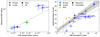 |
Fig. 20. Comparison between measured NIR and calculated stellar radii (left) and between the NIR and ALMA UD diameters (right). In each case, the dotted line represents a 1:1 relation. The dashed line in the right panel represents a fit to the measured AGB data points using orthogonal distance regression (Eq. (4)), with the grey region the uncertainty on this fit. The dot-dashed brown line shows the best linear fit for a relation forced to pass through the origin. See text for details. The shaded region in the right panel shows the uncertainty on the fit. The shaded region in the left panel shows that the measured NIR radii and the calculated radii for most stars fall within 15% of a 1:1 relation. |
Before comparing the calculated and NIR sizes with our new ALMA results, we first checked the available NIR diameters against the corresponding calculated radii. We converted the measured diameters to physical radii using the relation R★ = dθNIR/2 where the distance, d, was taken from Table 1 and θNIR is the NIR diameter. The uncertainties on the NIR radii come from the measurement uncertainties (Table 5) and the distance uncertainties (Table 1). The uncertainties on the calculated radii are probably lower limits since uncertainties for stellar effective temperatures and luminosities are not always provided in their literature sources. In the left panel of Fig. 20, we plot the NIR stellar radii against the calculated radii, assuming 15% uncertainties for the calculated sizes because the majority of stars are scattered around the 1:1 line to within 15% (grey shaded region). The exceptions are the significantly larger sources IRC+10011 and IRC−10529, which have larger measured radii than calculated, by factors of 1.5 and 2, respectively. This is most likely the result of optically thick dust found close to the star (Blasius et al. 2012).
In the right panel of Fig. 20 we plot the ALMA UD fit diameters against the measured NIR diameters (uniformly coloured markers), where available, or the calculated stellar diameters (grey filled markers) if there are no NIR measurements. The dotted line in Fig. 20 is for a 1:1 correspondence between the two measurements and we see that, in general, the ALMA diameters are larger than the NIR diameters.
We perform an orthogonal fit to only the AGB stars with measured (not calculated) NIR diameters and find the following relationship:
 (4)
(4)
where a = 1.22 ± 0.12 and b = 2.2 ± 1.5 mas. This relationship is plotted as the dashed line in the right panel of Fig. 20, with the uncertainties shown by the grey shaded region. Note that although IRC−10529 and IRC+10011 are outliers with larger NIR diameters than ALMA UD diameters, the uncertainties on their NIR radii are so large that they do not significantly contribute to the fit. With the exception of these two stars, there is minimal scatter around the trend line for the stars with measured data. There is more scatter among the stars with calculated optical diameters, but the only true outlier among these is RW Sco, for which uncertainties come from being unresolved by ALMA (resulting in an uncertain UD diameter; see Table 2) and an uncertain effective temperature estimate, as noted above.
Of course Eq. (4) must only be valid over a limited regime, since a non-zero diameter at one wavelength cannot physically correspond to a diameter of zero in another. However, in the right panel of Fig. 20 we plot observed sizes not physical sizes and the real lower limits on both axes are the resolution limits. Therefore, we must assume that this relationship only holds over a certain (apparent) size regime, or is not truly linear. To better understand this, we require a larger sample of high quality measurements in both the NIR and at 1.24 mm, ideally observed contemporaneously.
If, instead of allowing a general linear fit, we force the line to pass through the origin, we find a slope of 1.38, which is still a reasonable fit to the measured data and is shown as the dot-dashed brown line in Fig. 20. Plotting only calculated sizes for all the stars would result in even more scatter in our plot. This can partly be explained by the variations in temperature and radius at different phases of the pulsation period. Bojnordi Arbab et al. (2024) also showed that the theoretical sizes of AGB stars can vary across pulsation period, which would add to the scatter given that observations of different stars and different configurations were taken at different pulsation phases (e.g. see Table 7 of Baudry et al. 2023).
Finally, in addition to examining the observed sizes of our stars, we tested fitting the physical sizes. This introduces additional uncertainties from the distances but also has the effect of rearranging the data so that less weight is placed on the closest stars that have the largest apparent sizes but similar physical sizes to the majority of our sample. Within the uncertainties, a fit to these parameters results in a 1:1 relation between the ALMA- and NIR-derived physical sizes. (This holds whether or not we include the RSGs and/or the two largest AGB stars, IRC−10529 and IRC+10011, in our fit.) The results of this test indicate that the formal uncertainties on our fit (Eq. (3)) are smaller than the real uncertainties.
4.4. Trends between stellar properties
We checked for any trends between the measured continuum properties, based on the UD fits. In Fig. 21 we plot the monochromatic luminosity, which is essentially a normalised UD flux density, against the measured UD radii for our sample. The 1.24 mm radio luminosity, which we refer to as the monochromatic luminosity, was calculated using
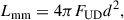 (5)
(5)
 |
Fig. 21. Monochromatic luminosities plotted against physical sizes, as calculated from the UD fits. Left: All the stars. Right: Stars within the dashed rectangle in the left panel. The error bars are omitted in this panel for clarity. The dotted vertical line is plotted at a radius of 2.95 × 1013 cm and separates the SR AGB stars from the Mira variables, as does the dotted horizontal line plotted at 1.2 × 10⁷ mJy pc2. |
where FUD is the UD flux density (Table 2), and d is the distance. The UD radius was calculated from the angular measurements given in Table 2, and the distances are listed in Table 1. We excluded RW Sco and KW Sgr from the comparison since their radii determined from the UD fits were very uncertain. In the left panel of Fig. 21 the dashed rectangle contains the majority of the ATOMIUM stars. We then used the limits of this box in the right panel to more clearly show the clustered data points. The stars that fall outside of the drawn box are the Mira variables IRC+10011 and IRC−10529, the RSGs VX Sgr and AH Sco, and SV Aqr. SV Aqr is both fainter and smaller than the other SR variables. The RSGs, IRC+10011, and IRC−10529 all have larger radii and higher fluxes than the rest of our sample. This is expected for the RSGs. IRC+10011 and IRC−10529 could be outliers because they are known to be very dusty and obscured AGB stars (e.g. both have high dust optical depths; Schöier et al. 2013).
No robust trend is seen for the SR AGB stars, although we note that all of the SR stars have radii < 3 × 1013 cm (< 2 au). They also all have monochromatic luminosities ≤1.2 × 10⁷ mJy pc2, whereas the Miras all have monochromatic luminosities > 1.2 × 10⁷ mJy pc2. The dotted vertical and horizontal lines in Fig. 21 illustrate these boundaries between the Miras and SRs. We see a general trend for the Miras of increasing flux with increased radius. The RSGs are both larger and more luminous than the AGB stars, which is to be expected as they are also more massive.
Considering all the stars plotted in Fig. 21, there is a clear positive correlation between the UD radius and the monochromatic luminosity. This is to be expected since the UD radius is related to the physical radius of the star (as discussed in Sect. 4.3) and the monochromatic luminosity has a dependence on the bolometric luminosity. Since the bolometric luminosity is proportional to the square of the physical radius (see Eq. (3)), it is then not surprising that a similar correlation would be reflected in the corresponding millimetre properties. A fit to these properties gives a slope close to 2, as expected for L★ ∝ R★2, but with large uncertainties owing to the scatter and uncertainties on our data.
4.5. Trends with period
We checked for any trends between the measured continuum properties and the pulsation period of the stars in our sample. The left panel in Fig. 22 shows the physical radii against the primary pulsation periods (Table 1) for our sample. The uncertainties on the radius include the distance uncertainties as well as the uncertainties on our UD fits. There is a positive trend for the Mira variable stars, which the two RSGs also broadly agree with. There is no trend for the SR AGB stars, which all have similar radii (as more clearly seen in Fig. 20) but a range of periods from 89 to 390 days. The only Mira that is an outlier is R Aql, partly because its distance is relatively uncertain (Andriantsaralaza et al. 2022), adding to the uncertainty in its radius. It is also the only Mira variable with a period < 300 days. The dashed black line is for a trend to the Mira data, excluding R Aql, for a relation between the 1.24 mm radius and the period:
 (6)
(6)
 |
Fig. 22. UD radii (left) and monochromatic fluxes (right) plotted against the pulsation period. The dashed black line in the left panel is a fit to the Mira variables. The dotted brown line in the right panel is a fit to the RSGs and the two Mira variables IRC−10529 and IRC+10011. |
with the RSGs found slightly above this trend line. If we assume that the Mira variables are all fundamental mode pulsators, this is in general agreement with the theoretical models of Ahmad et al. (2023) who found an increasing period with radius based on their CO5BOLD simulations.
In the right panel in Fig. 22 we plot the monochromatic luminosity (Eq. (5)) against the pulsation period. There is a positive relationship between the monochromatic luminosity and the period for the RSGs, with the two most extreme AGB stars (IRC−10529 and IRC+10011) agreeing with the trend seen for the RSGs. The dotted brown line plotted is for the relationship
 (7)
(7)
However, for the majority of the sample, we do not see any clear trends beyond what was already apparent from Fig. 21: the SR AGB stars have lower fluxes than the Miras. The Miras with periods ≤490 days all have comparable monochromatic luminosities with no correlation to the period. There is a weak positive correlation if we consider the two Miras with periods ≤490 days and SRs, but this arises from the fact that the SRs in our sample generally have shorter periods and all have lower monochromatic luminosities than the Miras. Figure 22 is quite different to period-luminosity diagrams constructed from bolometric luminosities or K-band absolute magnitudes (e.g. Whitelock et al. 2008; Trabucchi et al. 2017), which show much clearer trends for both Miras and SR variables.
Our results are in qualitative agreement with those of McDonald & Zijlstra (2016) who used infrared colour as a proxy for dust excess. They find a plateau in their period-colour plot from 120–300 days and an uptick at higher periods. The uptick in our period-monochromatic luminosity plot (right panel of Fig. 22) seems to occur at around 500 days rather than 300, but the turning point of a similar uptick in our period-radius plot (left panel of Fig. 22) occurs around 300–400 days.
5. Discussion
5.1. Dust features
With these observations, we present for the first time millimetre stellar and dust continuum emission at high angular resolution for a sizeable sample of AGB stars and RSGs. Where our ALMA continuum maps have been discussed phenomenologically in Sect. 3, we now focus on explanations for the observed dust distributions, including some comparisons between the ALMA continuum and observations from VLT/SPHERE Zurich Imaging Polarimeter (VLT/SPHERE-ZIMPOL; Beuzit et al. 2019; Schmid et al. 2018, hereafter referred to as SPHERE). Part of the ATOMIUM campaign involved contemporaneous (within 10 days) observations using the ALMA extended configuration and SPHERE. These have been published in detail by Montargès et al. (2023) and here we pay particular attention to the degree of linear polarisation (DoLP) plots in their Fig. 3. Note that the SPHERE images mainly show scattered light from dust grains located in the plane of the sky (see the discussion in Montargès et al. 2023), while our ALMA continuum images recover thermal emission from dust grains, in addition to the contribution to the continuum flux from the weak stellar photosphere/chromosphere and the radio photosphere as first described in Reid & Menten (1997) – see Sect. 5.2.
5.1.1. π1 Gru
In Fig. 23 we plot the contours of the combined π1 Gru continuum image over the DoLP image from Montargès et al. (2023). The tail seen in the combined continuum emission corresponds well to the tail seen in polarised flux. We also note that while the SPHERE image is contemporaneous with the extended ALMA observations, the tail requires the inclusion of the lower-resolution configurations, which were observed earlier than the extended configuration – extended was observed in June and July 2019, mid in October 2018, and compact in December 2018 and March 2019 (Gottlieb et al. 2022), while the SPHERE data were observed in July 2019 (Montargès et al. 2023). Therefore, the combined ALMA image is averaged over a longer period of time than the SPHERE image. Furthermore, the highest degree of polarisation is observed for dust with a 90° scattering angle, i.e. in the plane of the sky, whereas the continuum emission detected by ALMA does not have that limitation. This could explain why the emission seen to the N and NW of the AGB star is seen in the ALMA continuum but not in the DoLP map; it is not in the plane of the sky.
 |
Fig. 23. DoLP around π1 Gru observed with SPHERE (from Montargès et al. 2023) with the combined continuum contours observed with ALMA plotted in white (see Fig. 7), showing good agreement. The position of the AGB star is indicated by the large red cross, and that of the C companion by the smaller yellow cross. |
This tail of dust lies in the wake of the C companion of the π1 Gru system. By collecting archival SPHERE data, Montargès et al. (2025) have shown that the tail changes position as the companion orbits the AGB star with a period of 11 years. Subsequent ALMA observations have confirmed that the continuum feature associated with the C component also changes position in an orbit around the AGB star (Esseldeurs et al. 2025). Using hydrodynamic simulations, El Mellah et al. (2020) and Malfait et al. (2024) showed that not only do close companions to AGB stars shape the AGB wind into spiral patterns (especially when viewed face on, with the line of sight perpendicular to the orbital plane) but that accretion discs can also form around such companions. Montargès et al. (2025) presented a detailed analysis of the nature of the C companion, and concluded that the feature attributed to the C companion in the extended ALMA continuum likely originates from an accretion disc around the star (which may be a white dwarf or a K dwarf main sequence star).
Montargès et al. (2025) suggest that the dust tail is seen because dust is concentrated in the wake of the companion or that dust growth is accelerated in that region. Based on the observations presented here of π1 Gru and other stars (see the discussion on W Aql below) we suggest that dust preferentially forms in the wakes of shocks caused by companions moving supersonically through the AGB wind. Since the sound speed is relatively low, even in the inner wind (∼3 km s−1), the orbital velocity will almost always be supersonic for a companion within the AGB circumstellar envelope. This is the origin of the shock waves seen in hydrodynamic simulations of companion-wind interactions (e.g. Maes et al. 2021; Malfait et al. 2021, 2024). These shocked structures are denser than the surrounding gas, meaning that chemical reactions, including those involved in dust formation, can progress faster. This would also explain the dust distribution around IK Tau (see the discussion in Coenegrachts et al. 2023) and is in line with other theoretical modelling results that show that dust forms in the wake of shocks (Freytag & Höfner 2023). We ran a hydrodynamic model including dust formation to test this point and present some first results in Appendix H. A detailed theoretical study of binary-enhanced dust formation over a wider parameter space is forthcoming (Samaratunge et al., in prep.).
5.1.2. W Aql
W Aql has a known F9 main sequence companion presently at a separation of around 200 au (see the detailed discussion in Danilovich et al. 2024). In Fig. 4, continuum emission is detected close to the position of the companion with a confidence of 5σ. Since we know the nature of the F9 companion, we know that the star itself cannot account for that level of 1.24 mm emission. The hydrodynamic models in Danilovich et al. (2024) do not predict an accretion disc around such a distant companion5 (see also El Mellah et al. 2020), but they do predict a shocked wake close to the companion. The dust observed near the companion could hence be formed in its wake. If this is the case, then we are observing some dust formation ∼200 au from the AGB star. This is much further out than the dust condensation radius, estimated to be around 13 au by Danilovich et al. (2014), which is the approximate region within which all dust was previously thought to form.
The DoLP plot for W Aql in Montargès et al. (2023) shows large regions of polarised flux detected with high certainty; it has the highest DoLP of the ATOMIUM SPHERE sample. The polarised flux is seen on all sides of the AGB star, with the brightest region to the SSE. The position of the companion is just outside of the region of polarised flux. It may be contributing to the brighter polarised flux region in the SSW by providing additional illumination. The ALMA continuum flux is found in approximately the same general region as the SPHERE polarised flux, but does not follow the regions of highest polarisation.
Overall, we see dust close to the AGB star and further away at the position of the companion. The timescales of the wind expansion and the companion’s orbit strongly suggest that dust is forming in the vicinity of the AGB star and in the vicinity of the companion. If dust primarily forms in the wake of shocks, then what we see for W Aql is dust formation driven by two types of shocks: stellar pulsations close to the AGB star and the wake of the companion moving through the wind supersonically.
5.1.3. GY Aql
The bar seen in the GY Aql continuum images (Fig. 1) is found at a larger separation from the position of the star (extending out to ∼1″) than the DoLP SPHERE image presented in Montargès et al. (2023), where the majority of the DoLP flux is within 0.2″. The SPHERE image shows arcs of polarised flux around the star, especially to the S and NW. Figure 11 of Montargès et al. (2023) shows that the DoLP image may trace out some of the spiral pattern seen in the CO moment 1 map, which represents the velocity field. Since the CO channel maps reveal spiral-like patterns in the wind of GY Aql (Decin et al. 2020), it is not unreasonable to expect (some of) the dust to also follow the density structures in the wind. Unfortunately, at the separation of the bar structure from the AGB star, the velocity field is messy and it is difficult to draw conclusions through a simple comparison. A more detailed analysis of GY Aql is forthcoming in a separate paper (Marinho et al., in prep.).
5.1.4. SV Aqr
The continuum emission observed with ALMA towards SV Aqr (Fig. 5) appears to form an arc. The DoLP image presented in Montargès et al. (2023) has rather low S/N and only a small region of polarised flux above the 3σ detection threshold, located to the SE of the star and within ∼20 mas. This is too close to be resolved by the ALMA beam in the extended data, but is close to the asymmetry seen in the 3σ contour of the extended data. We reproduce the DoLP image over-plotted with the extended continuum contours in Fig. 24, but we caution against over-interpretation of this image, and direct the reader to the discussion of reliability in Montargès et al. (2023) and the 3σ contours plotted in their Fig. 3.
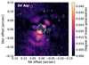 |
Fig. 24. DoLP around SV Aqr observed with SPHERE (from Montargès et al. 2023) with the extended continuum contours observed with ALMA plotted in white (see Fig. 5). The position of the AGB star is indicated by the green cross. |
Overall, the dust in the vicinity of SV Aqr follows an irregular pattern. It could be distributed in this way as a result of episodic dust formation, perhaps driven by asymmetric bubbles on the surface, similar to what is seen in the models of Freytag & Höfner (2023). Dust emission forming an arc or loop near the star could have been formed by a companion shaping the wind and/or enhancing dust in this region. We found SV Aqr to have an additional period of 231.8 days, with alternating cycles having minima of different depths (see Appendix A.1 for details). This could indicate a binary system with a period of 463.6 days. However, the feasibility of this strongly depends on the system mass. If the system mass is only 1 M⊙ (i.e. for a planetary or brown dwarf companion), then the separation for a circular orbit would be only 1.2 au, smaller than the radius we measured with ALMA, even considering our significant uncertainties. A system mass of 2 M⊙ or higher would place a companion (just) outside of our measured radius. Hence, the available evidence suggests a rather tight binary system. Since it is not presently interacting strongly, this further indicates a system mass ≥2 M⊙.
5.1.5. U Del
The other star in our sample with a long secondary period is U Del, with a secondary period of 1163 days (Speil 2006). It is the star with the least dust in our sample, especially away from the star, since there was no significant residual flux in our UD-subtracted image (Fig. 6). The spectrum of U Del has the fewest lines from the fewest different molecular carriers of all the stars in the ATOMIUM sample (Wallström et al. 2024; Baudry et al. 2023). The DoLP image of U Del in Montargès et al. (2023) shows very little polarised flux above the noise. This is evidence against the long secondary period being caused by a dust-shrouded companion (as described in Soszyński et al. 2021), since in that case we would expect to see more circumstellar dust in general; it is unlikely that a companion would accrete literally all the dust. However, as discussed by Goldberg et al. (2024), it is possible that a companion might be modulating the AGB dust in a different way. A final possibility is that a companion is accelerating the formation of the dust on a smaller scale than for π1 Gru; for example, if the companion has a much lower mass than π1 Gru C it could be undetected in our ALMA observations and only evident in the long secondary period.
5.1.6. KW Sgr
KW Sgr, a RSG that we did not observe with the compact configuration of ALMA, has a highly elliptical beam in the mid data and some small asymmetries in the continuum at levels of ∼3σ, but these asymmetries are generally smaller than the area of the beam and, hence, not significant. The UD-subtracted image (Fig. 15) shows some dust extending ESE of the continuum peak, with a confidence of 3σ, and a little more emission at the position of the continuum peak. Although this protrusion has a low S/N, it agrees well with a similar protrusion seen in the SPHERE DoLP presented by Montargès et al. (2023), although the DoLP feature also has a low S/N. To emphasise their similarity, we plot the UD-subtracted continuum contours over the SPHERE DoLP image in Fig. 25. The fact that two very different imaging techniques show a similar protrusion lends some credence to it. Given the high asymmetry of this feature, we suggest that it may be a result of episodic mass loss, which is thought to be characteristic of RSGs (e.g. see Levesque 2017, and references therein) and akin the phenomenon termed the Great Dimming of Betelgeuse (Montargès et al. 2021) and the episodic ejecta of VY CMa (Humphreys et al. 2024, 2025).
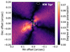 |
Fig. 25. DoLP around KW Sgr observed with SPHERE (from Montargès et al. 2023) with the UD-subtracted contours (at 3 and 5σ) observed with ALMA plotted in white (see Fig. 15). The emission from the two telescopes is in good agreement. The position of the AGB star is indicated by the green cross. |
5.1.7. VX Sgr and AH Sco
In the SPHERE observations presented in Montargès et al. (2023), the RSGs VX Sgr and AH Sco exhibit moderately extended regions of polarised flux. In both cases, especially AH Sco, the highlighted regions are partly limited by the S/N of the observations. That is, we see polarised flux mainly to the north and south of AH Sco with SPHERE but this is partly because the S/N to the east and west is worse, limiting our ability to compare with the significant ALMA flux to the east and west of AH Sco (Fig. 17, Sect. 3.5.6). For VX Sgr, there appears to be more polarised flux from SPHERE than extended emission from ALMA, but this is likely a result of ALMA resolving out some flux (see Sect. 3.4.3). The VLT/AMBER imaging of VX Sgr in the NIR by Chiavassa et al. (2010) also shows significant complexity in the atmosphere and within a radius of ∼10 mas. Chiavassa et al. (2010) tentatively show extended structures close to the star (∼10 mas) to the north and south. Our extended array observations (Fig. 16) show structures to the north and south out to ∼100 mas (∼160 au). If these are the same ejecta and we consider the difference in observation times (∼11 years), then the lower limit on the velocity of these features (ignoring projection effects) would be 60 km s−1, comparable to some of the high velocity jets seen for VY CMa, another extreme RSG (Quintana-Lacaci et al. 2023). If these are not the same structures, then their similarity across physical scales at different times are suggestive of localised episodic mass loss around VX Sgr. What we can conclude from the infrared and ALMA observations is that both VX Sgr and AH Sco have significant circumstellar dust, as has been shown by earlier observations of, for example, silicate features in infrared spectra (Speck et al. 2000).
5.2. Angular sizes at millimetre wavelengths
The apparent angular sizes of AGB stars at radio wavelengths are thought to be dominated by electron-neutral free-free emission out to ∼2 R★ (Reid & Menten 1997; Matthews et al. 2015; Vlemmings et al. 2019). The apparent size of this radio photosphere decreases with increasing frequencies, because of changes in opacity, resulting in apparent sizes < 1.5 R★ for ≳200 GHz (Vlemmings et al. 2019; Bojnordi Arbab et al. 2024). Prior to the present work, a few studies have examined the angular sizes of AGB stars at sub-millimetre, sub-millimetre, and longer radio wavelengths. Pertinent results of such studies are summarised in Table 7. To ensure a valid comparison between our measurements of angular sizes and those of earlier studies, we focus on the observations closest to the central frequency of our Band 6 continua (241.75 GHz or 1.24 mm). Vlemmings et al. (2019) studied four nearby oxygen-rich AGB stars – W Hya, o Cet (also known as Mira A), R Dor, and R Leo – at high angular resolution across multiple wavelength ranges. Higher-resolution observations of W Hya (Ohnaka et al. 2024) and R Dor (Vlemmings et al. 2024) are also available. Uniform discs were fit by the authors of these earlier observations, allowing us to directly compare the stellar properties to our sample.
Overview of UD measurements in the literature.
Of these four stars, R Dor is a SRb type variable, while W Hya, o Cet, and R Leo are all Mira variables. Situating them in our plot of monochromatic luminosity against UD radius in Fig. 21, we find that R Dor sits in the SR quadrant of the plot, with a lower flux and smaller radius than the Mira variables. The three Mira stars lie in the Mira quadrant, upholding the divisions we found. We also considered the pulsation periods of these stars and comparing with our plots of UD properties against period, extending Fig. 22 in Fig. B.4. We find that the Mira variables cluster close to the Miras in our sample (with periods of 402 days, 332 days and 310 days for W Hya, o Cet, and R Leo, respectively). R Dor has two periods of comparable length to T Mic (332 and 175 days for R Dor, Bedding et al. 1998, and 352 and 178 days for T Mic, Table 1), so sits near T Mic and S Pav on the plot of UD radius against period if we consider the longer period as the primary.
Asaki et al. (2023) present high angular resolution continuum images of the carbon-rich Mira variable R Lep, observed with ALMA Bands 8, 9, and 10. These are higher frequencies than our observations, but if we compare their Band 8 results (at 405.0 GHz, or 0.74 mm) with our data, we find that R Lep sits in the Mira quadrant of our Fig. 21, with a UD radius of 5 × 1013 cm and monochromatic luminosity of 1 × 10⁸ mJy pc2. The parameters of CW Leo, another carbon-rich Mira, measured by Velilla-Prieto et al. (2023) are also comparable to R Lep. However, those authors fit a Gaussian rather than a UD to their high angular resolution continuum image (observed with ALMA Band 6), so their results are not directly comparable to ours, especially when it comes to the measured radius.
Overall, these past studies agree very well with the trends between radius and period that we see in our sample. Aside from CW Leo, which is most likely an outlier because its size was determined from a Gaussian fit, the Mira variables lie near our trend line (Eq. (6)), within the uncertainties. Furthermore, when considering the longer period of R Dor, described as Mira-like by Bedding et al. (1998), it also agrees with the trend line (but we note that its smaller radius makes it more typical of the SR variables). When using the shorter period for R Dor, the star falls among the SR variables in the period-radius plot. There is also good agreement between the literature data and the general trends seen between period and monochromatic luminosity for the ATOMIUM sample. In this case, the main outlier is R Lep, having a larger monochromatic luminosity than other stars with similar periods, but this is probably because the observations were from Band 8 with a higher frequency, making them less directly comparable. We also note that now CW Leo lies close to IRC+10011 and IRC−10519, in agreement with our Eq. (7) line, which supports our hypothesis that the stars with the longest periods (> 500 days) agree with this trend.
In recent work, Vlemmings et al. (2024) measured the stellar disc of the closest AGB star, R Dor, with ALMA and compared this diameter with the NIR diameter measured by Ohnaka et al. (2019). For the ALMA radius at 225 GHz (1.33 mm, close to our 1.24 mm) the measurements of Vlemmings et al. (2024) and Ohnaka et al. (2019) agree well with our Eq. (4). They report for R Dor RUD = 1.22 ± 0.11 RNIR, which is the same gradient as in our Eq. (4), but passing through the origin. When we fit to our data but force the line to pass through the origin, we find a slope of 1.38. Both this result and the relation in Eq. (4) are close to being within the uncertainties of the Vlemmings et al. (2024) result for R Dor.
Through an analysis of theoretical models, Bojnordi Arbab et al. (2024) found a variation with pulsation phase of about ±20% for the observable radii at 231 GHz of the model AGB star. This would account for the scatter in our comparison between ALMA and NIR data, especially since (i) there is no consistency in the pulsation phase at which measurements were taken and (ii) even if there was, the phase at which the measured radii peak is expected to vary with wavelength, as discussed in detail by Bojnordi Arbab et al. (2024). Therefore, to more precisely study the relationship between radio and NIR sizes of AGB stars, high-resolution data would need to be taken contemporaneously. This is not possible to achieve with the contemporaneous SPHERE observations of Montargès et al. (2023), as the stars are mostly smaller than their corresponding point spread functions.
5.3. Two modes of dust formation: Pulsation- and binary-enhanced
We propose a second pathway for shock-driven dust formation. In addition to the well established pathway of stellar pulsations, we propose that the supersonic motion of companion stars through the circumstellar envelope enhances dust production. All stars in our sample exhibit some dust in the close stellar environment (even U Del, on the basis of its long secondary period; see Sect. 5.1.5). However, not all stars exhibit regions of continuum flux offset from the continuum peak. Excluding RW Sco6, all the stars with periods longer than 300 days have some resolved regions of continuum flux. For periods shorter than 300 days, only two unusual stars have notable regions of resolved flux: π1 Gru and SV Aqr, discussed above in Sects. 5.1.1 and 5.1.4, respectively. In both of these cases the dust emission offset from the continuum peak can be attributed to a known (π1 Gru) or a suspected companion (SV Aqr; see Appendix A.1).
5.3.1. Pulsation-enhanced dust formation
Pulsation periods of ≳300 days are thought to be necessary for an AGB star to fully develop a pulsation-enhanced dust-driven wind (Winters et al. 2000; McDonald & Zijlstra 2016), a hypothesis supported by observations of both oxygen-rich and carbon-rich stars, where a positive correlation between mass-loss rate and period is seen above 300 days (Groenewegen et al. 1998; Olofsson et al. 2002; Ramstedt et al. 2009; McDonald & Zijlstra 2016). This is also in agreement with the relation found by Wood (1990) for an exponential increase in mass-loss rate with pulsation period7, mainly holding between 300 and 500 day periods, above which the mass-loss rate no longer increases with period (Vassiliadis & Wood 1993).
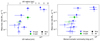 |
Fig. 26. Mass-loss rates plotted against physical sizes (left), as calculated from the UD fits, and monochromatic luminosities (right), for the AGB stars. The vertical error bars indicate assumed 50% uncertainties on the mass-loss rates. |
To check whether such a correlation holds for the ATOMIUM sample, we collected mass-loss rates from the literature, as described in Appendix G and listed in Table G.1. Since the ATOMIUM sample populates a period–mass-loss rate diagram too sparsely to draw conclusions, we supplement the data with the additional 37 stars from the SUbmilimetre Catalogue of Circumstellar EnvelopeS with Herschel/HIFI sample (SUCCESS; Danilovich et al. 2015b), including carbon stars. We plot the mass-loss rates against pulsation periods for the combined ATOMIUM and SUCCESS samples in Fig. G.1. We also plot the Wood (1990) relation for periods between 300 and 500 days (dashed brown line). The ATOMIUM stars with periods above 300 days agree with the underlying trend seen in the SUCCESS sample. Below 300 days, there is no trend. Above 500 days there may be a bimodal trend with one mode including most of the carbon stars and the longest-period S-type star, and the other mode including high mass-loss rate oxygen-rich stars and the carbon star II Lup.
McDonald & Zijlstra (2016) also noted that stars with pulsation periods above 500 days were the most extreme stars in the sample and included RSGs and known binaries. When considering the period–radius and period–monochromatic luminosity plots in Fig. 22, we see an uptick in radius among the Miras for periods above 300 days, possibly suggesting that longer pulsation periods correlate to larger radii as well as increased dust production for this period range. However, the uptick in monochromatic luminosity is only seen above ∼500 day periods, suggesting that it is only these most extreme stars that have higher millimetre luminosities. This could possibly be the result of the UD fits to the 5 extreme stars (two extreme and distant AGB stars and our RSG subsample) including more circumstellar dust than the closer stars in our sample. This is partly reflected in the rather low brightness temperatures obtained for IRC−10529 and AH Sco. Kiss et al. (2006) also noted that VX Sgr (and to a lesser extent AH Sco8) has a particularly large pulsation amplitude, which they associated with increased pulsation-enhanced mass loss and dust production. This fits with the finding by Freytag & Höfner (2023), based on their 3D theoretical models, that dust forms in the wake of shocks within a few stellar radii of the star; larger-amplitude pulsations would produce stronger shocks. All three RSGs in ATOMIUM agree well with a trend with pulsation period, even though KW Sgr appears to be the least dusty of the three (see the estimated dust mass in Table 4). IRC−10529 and IRC+10011 are also known to be extremely dusty (Justtanont et al. 2013; Reiter et al. 2015), which fits with the ‘extreme’ label noted by McDonald & Zijlstra (2016). From these observations we can hypothesise that for stars with periods above 300 days we see an increase in both the mass-loss rate and the millimetre radius, while for stars with periods above 500 days we see an increase in monochromatic luminosity and another increase in mass-loss rate.
To check this hypothesis, we also plotted mass-loss rates for the AGB stars against each of UD radius and monochromatic luminosity, as shown in Fig. 26. In both plots, the two more extreme sources, IRC−10529 and IRC+10011, sit apart from the rest of the sample, having the largest UD radius and monochromatic luminosity. For the other stars, there is a trend of increasing mass-loss rate with increasing UD radius and increasing monochromatic luminosity. This suggests that a maximum mass-loss rate has been reached by IRC−10529 and IRC+10011 (and perhaps GY Aql; see Table G.1), and further increases in UD radius, monochromatic luminosity and period (Fig. G.1) do not contribute to increases in mass-loss rate. Considering the SR variables only, there is no correlation between the mass-loss rate and the UD radius, nor between the mass-loss rate and the monochromatic luminosity.
5.3.2. Binary-enhanced dust formation
π1 Gru and R Aql have the two highest mass-loss rates for stars with periods below 300 days (Table G.1). For R Aql this can be explained by its declining period (Zhao-Geisler et al. 2012); in 1915 the period was ∼320 days, placing it within the trend of the other longer-period stars. The mass-loss rate calculated from CO lines is an average over several hundred years so will not have altered appreciably in that time. For π1 Gru, the gas mass-loss rate calculated by Doan et al. (2017) takes the complex circumstellar structure into account. The high mass-loss rate, compared with other stars with pulsation periods around 200 days, can be explained by the extra dust produced in the wake of the companion, which orbits with a semi-major axis of ∼7 au (approx. 3–4 stellar radii, Montargès et al. 2025; Esseldeurs et al. 2025). Once more dust is formed, radiation pressure from the AGB star will push it outwards with the rest of the dust. If it is within the wind acceleration region, this additional dust can enhance the mass loss as part of the dust-driven wind, since there will be more dust available to collide with and drag the gas outwards.
The 3D single star models of Freytag & Höfner (2023) show that some gas still falls back onto the star out to radii of ∼9 au, so additional dust produced within 9 au could contribute to enhanced mass-loss. This phenomenon could explain moderate mass-loss rates for the majority of surveyed SR stars with shorter periods (< 300 days). Because the shocks induced by the companion persist further out in the wind (e.g. in spiral patterns; see Appendix H and e.g. Kim et al. 2017, 2019; Malfait et al. 2021), some dust will also form well outside of the wind acceleration region (see the middle panel of Fig. H.1), and will increase the overall dust-to-gas ratio compared with that of an otherwise similar single star. This could also contribute to the over-estimation of mass-loss rates calculated from dust properties and assumed dust-to-gas ratios, and could explain the discrepancy between mass-loss rates calculated from dust and from CO for the dustiest stars (e.g. see the comparisons in Table 4 of Justtanont et al. 2006, where mass-loss rates from the two methods differ by around an order of magnitude).
Many surveys, including both ATOMIUM and SUCCESS, are biased towards stars that have previously been detected (strongly) in CO, meaning they are likely to have higher mass-loss rates. If single stars with short pulsation periods have low levels of dust production and low mass-loss rates (e.g. McDonald et al. 2018) they would be less likely to be included in biased surveys. This explains the apparently high prevalence of binary AGB stars judging by their CO morphologies in high-resolution ALMA observations (see also Sect. 5.4). An unbiased survey such as the Nearby Evolved Star Survey (NESS; Scicluna et al. 2022) is hence likely to include stars with much lower mass-loss rates than stars that have been more frequently studied for their brighter emission lines. Another example is the small fraction of dusty field stars with luminosities below the tip of the red giant branch (McDonald et al. 2012, 2017). These have been assumed to be the lowest-mass AGB stars, since they have similar luminosities to the lowest-luminosity dusty AGB stars in globular clusters (Boyer et al. 2009; McDonald et al. 2009, 2011). However, these could instead be stars that have dust production triggered by companions. The corollary to this would be that the AGB stars with the lowest mass-loss rates (perhaps < 1 × 10⁻⁸ M⊙ yr−1 or lower) are least likely to have close companions.
This principle of two dust production channels can also partly explain the scatter in the period–mass-loss rate diagram and perhaps the bimodal distribution for stars with periods longer than ∼500 days. If dust production and hence mass loss only depended on pulsation period, then we would expect to see minimal scatter beyond that caused by different types of dust forming around the different chemical types (oxygen-rich, carbon-rich, and S-type). Companions driving the formation of additional circumstellar dust can increase the dust production by different amounts depending on orbital configuration. For example, the companion to W Aql seems to have produced a relatively small trail of dust ∼200 au from the AGB star, while the closer companion to π1 Gru, at ∼6.5 au (Montargès et al. 2025) has produced a longer dust tail in its wake; compare Figs. 4 and 7. Hence, we can theorise that although the present contribution of W Aql B to the total dust budget is low, the companion will have temporarily driven dust formation more vigorously during its periastron passage, in addition to driving chemical diversity (Danilovich et al. 2024).
At 1 M⊙, around half of stars are expected to have companions with masses at least 10% that of the primary (Moe & Di Stefano 2017). The proportion of stars with such companions increases to over 100% for stars of 8 M⊙, meaning that some such stars are expected to be in triple systems. Close companions are more likely for higher-mass stars (Moe & Di Stefano 2017). However, the closer the companion, the more intense the shock waves generated as it travels through the wind and hence the more dust formation triggered, in addition to the pulsation-driven dust formation. This additional dust can enshroud the companion, making it more difficult to detect with optical telescopes. W Aql B suffers from ∼2 mag of extinction ∼200 au from the AGB star (Danilovich et al. 2015a) but can still be detected with Hubble and SPHERE (Ramstedt et al. 2011; Montargès et al. 2023). The close companion to π1 Gru has only been detected by the dust associated with it in the ATOMIUM continuum (Fig. 7 and Homan et al. 2020) and in scattered polarised light (Montargès et al. 2023, 2025). The optical light (whether the companion is a white dwarf or a main sequence star) has been completely attenuated by the dust.
π1 Gru is the second closest star in the ATOMIUM sample and the companion is only just resolved from the AGB continuum in the extended data. If the system were a little further away, or oriented less favourably, or the projected separation between the two stars a little smaller, then we would not be able to distinguish the companion from the AGB continuum flux. Therefore, we cannot rule out the presence of companions for the majority of the ATOMIUM sample just because we have not (yet) directly observed them. Unseen companions could partly explain the extended dust distributions seen for U Her, R Hya, and S Pav, as well as the less symmetric emission seen for GY Aql, R Aql, IRC−10529, SV Aqr, T Mic, and IRC+10011.
5.4. Other indications of binarity
Indirect evidence of AGB binarity has previously been found in resolved CO emission, including from the ATOMIUM data (Decin et al. 2020) and earlier studies of other stars such as R Scl (Maercker et al. 2012), CW Leo (Cernicharo et al. 2015), and AFGL 3068 (Kim et al. 2017). Such structures can be reproduced – or partially reproduced – through hydrodynamic modelling (e.g. Mastrodemos & Morris 1998, 1999; Kim et al. 2019; El Mellah et al. 2020; Malfait et al. 2021). Molecular signatures can also be used to indirectly infer the presence of UV-emitting binaries (Van de Sande & Millar 2022; Siebert et al. 2022; Danilovich et al. 2024). Studies that surveyed AGB stars in the UV or X-ray have detected emission for some stars (e.g. Ramstedt et al. 2012; Sahai et al. 2015; Ortiz & Guerrero 2021; Schmitt et al. 2024) that likely does not come from the AGB star itself. This emission is thought to arise from companion stars, most likely from accretion discs that have formed around the companions (Sahai et al. 2015). None of the stars in the ATOMIUM sample are included in the aforementioned studies as confirmed detections9.
Out of the 14 AGB stars in the ATOMIUM sample, we have suggested that 11 of them might have binary companions, 9 of which have not been directly detected. Given that the ATOMIUM sample was selected to cover a range of mass-loss rates and pulsation behaviours (Gottlieb et al. 2022), there was no particular expectation for the stars to have binary companions. Population statistics indicate that at least half of stars in the AGB mass range should have companions (Moe & Di Stefano 2017), so earlier assumptions that the majority of AGB stars are single stars (i.e. before the advent of resolved imaging of the circumstellar environments) are statistically unlikely.
Recent data and developments from Gaia have allowed us to better constrain distances and infer the presence of companions (including some that can be resolved; Kervella et al. 2022). Based on the results of Kervella et al. (2022), Montargès et al. (2023) used a proper motion analysis combining Gaia Early Data Release 3 and HIPPARCOS data to estimate the probability of detecting close companions around the AGB stars. Note that the proper motion anomaly is not sensitive to wide binaries. They determine that GY Aql, R Aql, π1 Gru, and R Hya likely have a detectable close companion based on the large S/N of the proper motion anomaly, in agreement with our predictions.
6. Summary and conclusions
We present the continuum data observed for a sample of 14 AGB stars and 3 RSGs as part of the ATOMIUM ALMA large programme. For each star, we show the continuum observations from each individual array configuration as well as the combined image. Different features are apparent on different scales, owing to different resolutions, MRSs, and noise levels. We identify stars with extended continuum emission on scales of tens to hundreds of au, elongated structures, and a few unique structures. Notably, we see a tail of dust in the wake of the close companion of π1 Gru and some dust forming in the wake of the distant companion of W Aql. In addition to the main ALMA array data, we present new observations taken at lower frequencies and lower resolutions with the ACA for a subsample of 7 AGB stars.
For each star, we fitted UDs to the compact emission at the continuum peaks, which is dominated by the stellar flux but, for some stars, likely includes contributions from dust located close to the stellar surface. We present residual images after subtracting the UDs from the combined continuum maps, many of which better highlight the emission offset from the continuum peaks.
We compared the UD sizes and flux densities with stellar properties such as pulsation periods and mass-loss rates. Among the AGB stars, we find that all the SR variables in our sample have lower monochromatic luminosities and smaller UD radii than the Mira variables. As expected, the RSGs have even larger radii and higher monochromatic luminosities than the Mira variables. There is an overall correlation between the UD radii and monochromatic luminosities, as is expected from the general relationship between luminosity and radius.
Comparing our newly derived stellar properties with literature data, we find a linear relationship between ALMA stellar diameters at 1.24 mm and diameters obtained from NIR observations. For the SR variables, there is no correlation between their pulsation periods and their radii, nor between their pulsation periods and their monochromatic luminosities. For the Mira variables whose periods are longer than 300 days, there is a positive trend between periods and radii, which matches a previously found uptick in dust production for periods above 300 days. There is a positive trend between monochromatic luminosities and periods for the RSGs and the two AGB stars with the highest fluxes, but no clear trend for the other AGB stars. This may correspond to extreme dust production being seen for stars with pulsation periods of more than 500 days.
Comparing the ATOMIUM sample to the larger SUCCESS survey, we find that among SR stars with low periods, π1 Gru has an especially high mass-loss rate; we conclude this is likely because of the additional dust forming in the wake of the shocks generated by the passage of its close companion. Hence, we propose two channels for dust formation around AGB stars: in the wake of shocks caused by pulsations and in the wake of shocks caused by the supersonic passage of a companion through the circumstellar envelope. Consequently, we propose that dust emission at millimetre wavelengths, offset from the continuum peak and showing coherent structure that is, for example, reminiscent of a wake or shock, could be an indirect indicator of binarity. Deeper observations, which can detect low-surface-brightness features, for more stars with known binary companions are needed to confirm this hypothesis.
Data availability
The appendices to this paper can be found on Zenodo: https://doi.org/10.5281/zenodo.17292735. The observational data used here are openly available through the ALMA Science Archive: https://almascience.nrao.edu/aq/. The images, other data products and scripts for the standard data processing are available from the ATOMIUM Landing Page in the ALMA Science Archive: https://almascience.eso.org/alma-data/lp/atomium. The fully aligned images and other custom ALMA data products that were produced for this study are available at: https://doi.org/10.5281/zenodo.17015654.
AAVSO: www.aavso.org
Dynamic range is (peak flux)/(rms).
Note that this is a slightly different value than for the combined array data because fewer spectral windows were observed with the compact configuration than with the extended and mid configurations; see Gottlieb et al. (2022) for details.
Though we note this could be because those models do not include cooling; see the discussion in Malfait et al. (2024).
RW Sco is moderately distant (560 pc) and, in general, has a lower signal to noise than the majority of our sample, so it is possible that our observations were not sensitive enough to detect or resolve regions of extended flux.
The relation found by Wood (1990) is log Ṁ = −11.4 + 0.0125 P.
Note also that the Kiss et al. (2006) sample did not include KW Sgr.
Schmitt et al. (2024) include three ATOMIUM stars (π1 Gru, R Hya, and S Pav) in their list of surveyed stars, but note optical contamination, which cannot be disentangled from potential X-ray detections, making their results for these stars ambiguous.
Acknowledgments
We thank the anonymous referee for their careful reading and thoughtful comments on the manuscript. TD and NS are supported in part by the Australian Research Council through a Discovery Early Career Researcher Award (DE230100183). TC acknowledges funding from the Research Foundation – Flanders (FWO), grant 1166724N. LD and CL acknowledge support from the KU Leuven C1 excellence grant BRAVE C16/23/009. LD acknowledges support from KU Leuven Methusalem grant SOUL METH/24/012, and the FWO research grants G099720N and G0B3823N. FDC is a Postdoctoral Research Fellow of the Research Foundation – Flanders (FWO), grant 1253223N. IEM acknowledges support from ANID/FONDECYT, grant 11240206 ME acknowledges funding from the FWO research grants G099720N and G0B3823N. TJM acknowledges support from STFC grant no. ST/T000198/1 HSPM thanks the Deutsche Forschungsgemeinschaft (DFG) for support through the collaborative research center SFB 1601 (project ID 500700252) subprojects A4 and Inf. JMCP was supported by STFC grant number ST/T000287/1. DP acknowledges Australian Research Council funding via DP220103767. We also thank the Australia French Association for Research and Innovation (AFRAN) for financially supporting the 5th Phantom users workshop. RS’s contribution to the research described in this publication was carried out at the Jet Propulsion Laboratory, California Institute of Technology, under a contract with NASA. RS thanks NASA for financial support via GALEX GO and ADAP awards. LS is an FNRS senior researcher. MVdS acknowledges the Oort Fellowship at Leiden Observatory. OV acknowledges funding from the Research Foundation – Flanders (FWO), grant 1173025N. KTW acknowledges support from the European Research Council (ERC) under the European Union’s Horizon 2020 Research and Innovation programme (grant agreement number 883867, project EXWINGS). This work is funded by the French National Research Agency (ANR) project PEPPER (ANR-20-CE31-0002). We thank the Australian-French Association for Research and Innovation (AFRAN) for financial support. The research leading to these results has received funding from the European Research Council (ERC) under the European Union’s Horizon 2020 research and innovation program (project UniverScale, grant agreement 951549). This paper makes use of the following ALMA data: ADS/JAO.ALMA#2018.1.00659.L and 2019.1.00187.S. ALMA is a partnership of ESO (representing its member states), NSF (USA) and NINS (Japan), together with NRC (Canada), MOST and ASIAA (Taiwan), and KASI (Republic of Korea), in cooperation with the Republic of Chile. The Joint ALMA Observatory is operated by ESO, AUI/NRAO and NAOJ. We acknowledge excellent support from the UK ALMA Regional Centre (UK ARC), which is hosted by the Jodrell Bank Centre for Astrophysics (JBCA) at the University of Manchester. The UK ARC Node is supported by STFC Grant ST/P000827/1. Part of this work was performed on the OzSTAR national facility at Swinburne University of Technology. The OzSTAR program receives funding in part from the Astronomy National Collaborative Research Infrastructure Strategy (NCRIS) allocation provided by the Australian Government, and from the Victorian Higher Education State Investment Fund (VHESIF) provided by the Victorian Government. This research has made use of the SIMBAD database and the VizieR catalogue access tool, CDS, Strasbourg Astronomical Observatory, France (Wenger et al. 2000; Ochsenbein et al. 2000). This research has made use of the International Variable Star Index (VSX) database, operated at AAVSO, Cambridge, Massachusetts, USA. This research made use of Astropy (Astropy Collaboration 2013, 2018), SciPy (Virtanen et al. 2020), Matplotlib (Hunter 2007) and NumPy (Harris et al. 2020).
References
- Ahmad, A., Freytag, B., & Höfner, S. 2023, A&A, 669, A49 [NASA ADS] [CrossRef] [EDP Sciences] [Google Scholar]
- Altenhoff, W. J., Thum, C., & Wendker, H. J. 1994, A&A, 281, 161 [NASA ADS] [Google Scholar]
- Andriantsaralaza, M., Ramstedt, S., Vlemmings, W. H. T., & De Beck, E. 2022, A&A, 667, A74 [NASA ADS] [CrossRef] [EDP Sciences] [Google Scholar]
- Arroyo-Torres, B., Wittkowski, M., Marcaide, J. M., & Hauschildt, P. H. 2013, A&A, 554, A76 [NASA ADS] [CrossRef] [EDP Sciences] [Google Scholar]
- Asaki, Y., Maud, L. T., Francke, H., et al. 2023, ApJ, 958, 86 [NASA ADS] [Google Scholar]
- Astropy Collaboration (Robitaille, T. P., et al.) 2013, A&A, 558, A33 [NASA ADS] [CrossRef] [EDP Sciences] [Google Scholar]
- Astropy Collaboration (Price-Whelan, A. M., et al.) 2018, AJ, 156, 123 [Google Scholar]
- Bailer-Jones, C. A. L., Rybizki, J., Fouesneau, M., Demleitner, M., & Andrae, R. 2021, AJ, 161, 147 [Google Scholar]
- Baudry, A., Wong, K. T., Etoka, S., et al. 2023, A&A, 674, A125 [NASA ADS] [CrossRef] [EDP Sciences] [Google Scholar]
- Bedding, T. R., Zijlstra, A. A., Jones, A., & Foster, G. 1998, MNRAS, 301, 1073 [NASA ADS] [CrossRef] [Google Scholar]
- Beuzit, J. L., Vigan, A., Mouillet, D., et al. 2019, A&A, 631, A155 [NASA ADS] [CrossRef] [EDP Sciences] [Google Scholar]
- Blasius, T. D., Monnier, J. D., Tuthill, P. G., Danchi, W. C., & Anderson, M. 2012, MNRAS, 426, 2652 [Google Scholar]
- Bojnordi Arbab, B., Vlemmings, W., Khouri, T., & Höfner, S. 2024, ApJ, 976, 138 [Google Scholar]
- Boyer, M. L., McDonald, I., van Loon, J. T., et al. 2009, ApJ, 705, 746 [CrossRef] [Google Scholar]
- Cernicharo, J., Marcelino, N., Agúndez, M., & Guélin, M. 2015, A&A, 575, A91 [NASA ADS] [CrossRef] [EDP Sciences] [Google Scholar]
- Chen, X., & Shen, Z.-Q. 2008, ApJ, 681, 1574 [NASA ADS] [CrossRef] [Google Scholar]
- Chen, X., Shen, Z.-Q., & Xu, Y. 2007, Chin. J. Astron. Astrophys., 7, 531 [Google Scholar]
- Chiavassa, A., Lacour, S., Millour, F., et al. 2010, A&A, 511, A51 [NASA ADS] [CrossRef] [EDP Sciences] [Google Scholar]
- Coenegrachts, A., Danilovich, T., De Ceuster, F., & Decin, L. 2023, A&A, 678, A85 [NASA ADS] [CrossRef] [EDP Sciences] [Google Scholar]
- Cohen, M., Van Winckel, H., Bond, H. E., & Gull, T. R. 2004, AJ, 127, 2362 [NASA ADS] [CrossRef] [Google Scholar]
- Cortes, P., Vlahakis, C., Hales, A., et al. 2023, https://doi.org/10.5281/zenodo.7822943 [Google Scholar]
- Cox, N. L. J., Kerschbaum, F., van Marle, A.-J., et al. 2012, A&A, 537, A35 [NASA ADS] [CrossRef] [EDP Sciences] [Google Scholar]
- Danilovich, T., Bergman, P., Justtanont, K., et al. 2014, A&A, 569, A76 [NASA ADS] [CrossRef] [EDP Sciences] [Google Scholar]
- Danilovich, T., Olofsson, G., Black, J. H., Justtanont, K., & Olofsson, H. 2015a, A&A, 574, A23 [NASA ADS] [CrossRef] [EDP Sciences] [Google Scholar]
- Danilovich, T., Teyssier, D., Justtanont, K., et al. 2015b, A&A, 581, A60 [NASA ADS] [CrossRef] [EDP Sciences] [Google Scholar]
- Danilovich, T., Malfait, J., Van de Sande, M., et al. 2024, Nat. Astron., 8, 308 [CrossRef] [Google Scholar]
- Decin, L. 2021, ARA&A, 59, 337 [NASA ADS] [CrossRef] [Google Scholar]
- Decin, L., Montargès, M., Richards, A. M. S., et al. 2020, Science, 369, 1497 [Google Scholar]
- Dehaes, S., Groenewegen, M. A. T., Decin, L., et al. 2007, MNRAS, 377, 931 [NASA ADS] [CrossRef] [Google Scholar]
- Doan, L., Ramstedt, S., Vlemmings, W. H. T., et al. 2017, A&A, 605, A28 [NASA ADS] [CrossRef] [EDP Sciences] [Google Scholar]
- Dyck, H. M., Benson, J. A., van Belle, G. T., & Ridgway, S. T. 1996, AJ, 111, 1705 [NASA ADS] [CrossRef] [Google Scholar]
- El Mellah, I., Bolte, J., Decin, L., Homan, W., & Keppens, R. 2020, A&A, 637, A91 [NASA ADS] [CrossRef] [EDP Sciences] [Google Scholar]
- Esseldeurs, M., Decin, L., De Ridder, J., & ATOMIUM Consortium 2025, Nat. Astron., in press [Google Scholar]
- Feast, M. W. 1953, MNRAS, 113, 510 [NASA ADS] [CrossRef] [Google Scholar]
- Freytag, B., & Höfner, S. 2023, A&A, 669, A155 [NASA ADS] [CrossRef] [EDP Sciences] [Google Scholar]
- Gaia Collaboration (Brown, A. G. A., et al.) 2021, A&A, 649, A1 [NASA ADS] [CrossRef] [EDP Sciences] [Google Scholar]
- Gaia Collaboration (Arenou, F., et al.) 2023, A&A, 674, A34 [CrossRef] [EDP Sciences] [Google Scholar]
- Goldberg, J. A., Joyce, M., & Molnár, L. 2024, ApJ, 977, 35 [Google Scholar]
- Gottlieb, C. A., Decin, L., Richards, A. M. S., et al. 2022, A&A, 660, A94 [CrossRef] [EDP Sciences] [Google Scholar]
- Greaves, J., & Howarth, J. J. 2000, JBAA, 110, 131 [Google Scholar]
- Groenewegen, M. A. T., Whitelock, P. A., Smith, C. H., & Kerschbaum, F. 1998, MNRAS, 293, 18 [NASA ADS] [CrossRef] [Google Scholar]
- Groenewegen, M. A. T., Baas, F., Blommaert, J. A. D. L., et al. 1999, A&AS, 140, 197 [NASA ADS] [CrossRef] [EDP Sciences] [Google Scholar]
- Groenewegen, M. A. T., Barlow, M. J., Blommaert, J. A. D. L., et al. 2012, A&A, 543, L8 [NASA ADS] [CrossRef] [EDP Sciences] [Google Scholar]
- Guandalini, R., & Busso, M. 2008, A&A, 488, 675 [NASA ADS] [CrossRef] [EDP Sciences] [Google Scholar]
- Harris, C. R., Millman, K. J., van der Walt, S. J., et al. 2020, Nature, 585, 357 [NASA ADS] [CrossRef] [Google Scholar]
- Hashimoto, O., Izumiura, H., Kester, D. J. M., & Bontekoe, T. R. 1998, A&A, 329, 213 [NASA ADS] [Google Scholar]
- Hofmann, K. H., Beckmann, U., Blöcker, T., et al. 2002, New Astron., 7, 9 [Google Scholar]
- Höfner, S., & Freytag, B. 2019, A&A, 623, A158 [NASA ADS] [CrossRef] [EDP Sciences] [Google Scholar]
- Höfner, S., & Olofsson, H. 2018, A&ARv, 26, 1 [Google Scholar]
- Homan, W., Montargès, M., Pimpanuwat, B., et al. 2020, A&A, 644, A61 [NASA ADS] [CrossRef] [EDP Sciences] [Google Scholar]
- Homan, W., Pimpanuwat, B., Herpin, F., et al. 2021, A&A, 651, A82 [NASA ADS] [CrossRef] [EDP Sciences] [Google Scholar]
- Hony, S., Heras, A. M., Molster, F. J., & Smolders, K. 2009, A&A, 501, 609 [NASA ADS] [CrossRef] [EDP Sciences] [Google Scholar]
- Humphreys, R. M., Strecker, D. W., & Ney, E. P. 1972, ApJ, 172, 75 [NASA ADS] [CrossRef] [Google Scholar]
- Humphreys, R. M., Richards, A. M. S., Davidson, K., et al. 2024, AJ, 167, 94 [NASA ADS] [CrossRef] [Google Scholar]
- Humphreys, R. M., Jones, T. J., Davidson, K., et al. 2025, AJ, 169, 230 [Google Scholar]
- Hunter, J. D. 2007, Comput. Sci. Eng., 9, 90 [NASA ADS] [CrossRef] [Google Scholar]
- Izumiura, H., Hashimoto, O., Kawara, K., Yamamura, I., & Waters, L. B. F. M. 1996, A&A, 315, L221 [NASA ADS] [Google Scholar]
- Jayasinghe, T., Stanek, K. Z., Kochanek, C. S., et al. 2019, MNRAS, 486, 1907 [NASA ADS] [Google Scholar]
- Joyce, M., Molnár, L., Cinquegrana, G., et al. 2024, ApJ, 971, 186 [Google Scholar]
- Justtanont, K., Olofsson, G., Dijkstra, C., & Meyer, A. W. 2006, A&A, 450, 1051 [CrossRef] [EDP Sciences] [Google Scholar]
- Justtanont, K., Teyssier, D., Barlow, M. J., et al. 2013, A&A, 556, A101 [NASA ADS] [CrossRef] [EDP Sciences] [Google Scholar]
- Karakas, A. I., & Lugaro, M. 2016, ApJ, 825, 26 [NASA ADS] [CrossRef] [Google Scholar]
- Kervella, P., Arenou, F., & Thévenin, F. 2022, A&A, 657, A7 [NASA ADS] [CrossRef] [EDP Sciences] [Google Scholar]
- Khouri, T., Vlemmings, W. H. T., Paladini, C., et al. 2020, A&A, 635, A200 [NASA ADS] [CrossRef] [EDP Sciences] [Google Scholar]
- Kim, H., Trejo, A., Liu, S.-Y., et al. 2017, Nat. Astron., 1, 0060 [Google Scholar]
- Kim, H., Liu, S.-Y., & Taam, R. E. 2019, ApJS, 243, 35 [Google Scholar]
- Kiss, L. L., Szabó, G. M., & Bedding, T. R. 2006, MNRAS, 372, 1721 [Google Scholar]
- Knapp, G. R., Sandell, G., & Robson, E. I. 1993, ApJS, 88, 173 [Google Scholar]
- Kobayashi, C., Karakas, A. I., & Lugaro, M. 2020, ApJ, 900, 179 [Google Scholar]
- Levesque, E. M. 2017, Astrophysics of Red Supergiants (IOP Publishing) [Google Scholar]
- Li, A., & Draine, B. T. 2001, ApJ, 554, 778 [Google Scholar]
- Maercker, M., Mohamed, S., Vlemmings, W. H. T., et al. 2012, Nature, 490, 232 [NASA ADS] [CrossRef] [Google Scholar]
- Maercker, M., Khouri, T., Mecina, M., & De Beck, E. 2022, A&A, 663, A64 [NASA ADS] [CrossRef] [EDP Sciences] [Google Scholar]
- Maes, S., Homan, W., Malfait, J., et al. 2021, A&A, 653, A25 [NASA ADS] [CrossRef] [EDP Sciences] [Google Scholar]
- Malfait, J., Homan, W., Maes, S., et al. 2021, A&A, 652, A51 [NASA ADS] [CrossRef] [EDP Sciences] [Google Scholar]
- Malfait, J., Siess, L., Esseldeurs, M., et al. 2024, A&A, 691, A84 [Google Scholar]
- Martí-Vidal, I., Vlemmings, W. H. T., Muller, S., & Casey, S. 2014, A&A, 563, A136 [Google Scholar]
- Mastrodemos, N., & Morris, M. 1998, ApJ, 497, 303 [Google Scholar]
- Mastrodemos, N., & Morris, M. 1999, ApJ, 523, 357 [Google Scholar]
- Matthews, L. D., Reid, M. J., & Menten, K. M. 2015, ApJ, 808, 36 [Google Scholar]
- Mayer, A., Jorissen, A., Paladini, C., et al. 2014, A&A, 570, A113 [NASA ADS] [CrossRef] [EDP Sciences] [Google Scholar]
- McDonald, I., & Zijlstra, A. A. 2016, ApJ, 823, L38 [NASA ADS] [CrossRef] [Google Scholar]
- McDonald, I., van Loon, J. T., Decin, L., et al. 2009, MNRAS, 394, 831 [CrossRef] [Google Scholar]
- McDonald, I., Boyer, M. L., van Loon, J. T., et al. 2011, ApJS, 193, 23 [NASA ADS] [CrossRef] [Google Scholar]
- McDonald, I., Zijlstra, A. A., & Boyer, M. L. 2012, MNRAS, 427, 343 [Google Scholar]
- McDonald, I., Zijlstra, A. A., & Watson, R. A. 2017, MNRAS, 471, 770 [Google Scholar]
- McDonald, I., De Beck, E., Zijlstra, A. A., & Lagadec, E. 2018, MNRAS, 481, 4984 [NASA ADS] [CrossRef] [Google Scholar]
- Mel’Nik, A. M., & Dambis, A. K. 2009, MNRAS, 400, 518 [Google Scholar]
- Moe, M., & Di Stefano, R. 2017, ApJS, 230, 15 [Google Scholar]
- Monnier, J. D., Millan-Gabet, R., Tuthill, P. G., et al. 2004, ApJ, 605, 436 [NASA ADS] [CrossRef] [Google Scholar]
- Montargès, M., Cannon, E., Lagadec, E., et al. 2021, Nature, 594, 365 [Google Scholar]
- Montargès, M., Cannon, E., de Koter, A., et al. 2023, A&A, 671, A96 [NASA ADS] [CrossRef] [EDP Sciences] [Google Scholar]
- Montargès, M., Malfait, J., Esseldeurs, M., et al. 2025, A&A, 699, A22 [NASA ADS] [CrossRef] [EDP Sciences] [Google Scholar]
- Murakawa, K., Yates, J. A., Richards, A. M. S., & Cohen, R. J. 2003, MNRAS, 344, 1 [Google Scholar]
- Ochsenbein, F., Bauer, P., & Marcout, J. 2000, A&AS, 143, 23 [NASA ADS] [CrossRef] [EDP Sciences] [Google Scholar]
- O’Gorman, E., Vlemmings, W., Richards, A. M. S., et al. 2015, A&A, 573, L1 [NASA ADS] [CrossRef] [EDP Sciences] [Google Scholar]
- Ohnaka, K., Weigelt, G., & Hofmann, K. H. 2016, A&A, 589, A91 [NASA ADS] [CrossRef] [EDP Sciences] [Google Scholar]
- Ohnaka, K., Weigelt, G., & Hofmann, K.-H. 2019, ApJ, 883, 89 [NASA ADS] [CrossRef] [Google Scholar]
- Ohnaka, K., Wong, K. T., Weigelt, G., & Hofmann, K. H. 2024, A&A, 691, L14 [NASA ADS] [CrossRef] [EDP Sciences] [Google Scholar]
- Olofsson, H., González Delgado, D., Kerschbaum, F., & Schöier, F. L. 2002, A&A, 391, 1053 [NASA ADS] [CrossRef] [EDP Sciences] [Google Scholar]
- Ortiz, R., & Guerrero, M. A. 2021, ApJ, 912, 93 [Google Scholar]
- Paladini, C., Klotz, D., Sacuto, S., et al. 2017, A&A, 600, A136 [NASA ADS] [CrossRef] [EDP Sciences] [Google Scholar]
- Paladini, C., Baron, F., Jorissen, A., et al. 2018, Nature, 553, 310 [NASA ADS] [CrossRef] [Google Scholar]
- Pojmanski, G. 2002, Acta Astron., 52, 397 [NASA ADS] [Google Scholar]
- Quintana-Lacaci, G., Velilla-Prieto, L., Agúndez, M., et al. 2023, A&A, 669, A56 [NASA ADS] [CrossRef] [EDP Sciences] [Google Scholar]
- Ramstedt, S., & Olofsson, H. 2014, A&A, 566, A145 [NASA ADS] [CrossRef] [EDP Sciences] [Google Scholar]
- Ramstedt, S., Schöier, F. L., & Olofsson, H. 2009, A&A, 499, 515 [NASA ADS] [CrossRef] [EDP Sciences] [Google Scholar]
- Ramstedt, S., Maercker, M., Olofsson, G., Olofsson, H., & Schöier, F. L. 2011, A&A, 531, A148 [NASA ADS] [CrossRef] [EDP Sciences] [Google Scholar]
- Ramstedt, S., Montez, R., Kastner, J., & Vlemmings, W. H. T. 2012, A&A, 543, A147 [NASA ADS] [CrossRef] [EDP Sciences] [Google Scholar]
- Ramstedt, S., Vlemmings, W. H. T., Doan, L., et al. 2020, A&A, 640, A133 [EDP Sciences] [Google Scholar]
- Reid, M. J., & Menten, K. M. 1997, ApJ, 476, 327 [NASA ADS] [CrossRef] [Google Scholar]
- Reiter, M., Marengo, M., Hora, J. L., & Fazio, G. G. 2015, MNRAS, 447, 3909 [Google Scholar]
- Richichi, A., & Percheron, I. 2002, A&A, 386, 492 [NASA ADS] [CrossRef] [EDP Sciences] [Google Scholar]
- Sahai, R., Sanz-Forcada, J., Sánchez Contreras, C., & Stute, M. 2015, ApJ, 810, 77 [NASA ADS] [CrossRef] [Google Scholar]
- Schmid, H. M., Bazzon, A., Roelfsema, R., et al. 2018, A&A, 619, A9 [NASA ADS] [CrossRef] [EDP Sciences] [Google Scholar]
- Schmitt, J. H. M. M., Hünsch, M., Schneider, P. C., et al. 2024, A&A, 688, A9 [NASA ADS] [CrossRef] [EDP Sciences] [Google Scholar]
- Schöier, F. L., Ramstedt, S., Olofsson, H., et al. 2013, A&A, 550, A78 [Google Scholar]
- Scicluna, P., Kemper, F., McDonald, I., et al. 2022, MNRAS, 512, 1091 [NASA ADS] [CrossRef] [Google Scholar]
- Shappee, B. J., Prieto, J. L., Grupe, D., et al. 2014, ApJ, 788, 48 [Google Scholar]
- Siebert, M. A., Van de Sande, M., Millar, T. J., & Remijan, A. J. 2022, ApJ, 941, 90 [NASA ADS] [CrossRef] [Google Scholar]
- Sloan, G. C., Kraemer, K. E., McDonald, I., et al. 2016, ApJ, 826, 44 [NASA ADS] [CrossRef] [Google Scholar]
- Smak, J. 1964, ApJS, 9, 141 [Google Scholar]
- Soszyński, I., Olechowska, A., Ratajczak, M., et al. 2021, ApJ, 911, L22 [CrossRef] [Google Scholar]
- Speck, A. K., Barlow, M. J., Sylvester, R. J., & Hofmeister, A. M. 2000, A&AS, 146, 437 [NASA ADS] [CrossRef] [EDP Sciences] [Google Scholar]
- Speil, J. 2006, JAAVSO, 35, 88 [Google Scholar]
- Suh, K.-W. 1999, MNRAS, 304, 389 [NASA ADS] [CrossRef] [Google Scholar]
- The CASA Team, Bean, B., Bhatnagar, S., et al. 2022, PASP, 134, 114501 [NASA ADS] [CrossRef] [Google Scholar]
- Trabucchi, M., Wood, P. R., Montalbán, J., et al. 2017, ApJ, 847, 139 [Google Scholar]
- Ueta, T., Speck, A. K., Stencel, R. E., et al. 2006, ApJ, 648, L39 [Google Scholar]
- van Belle, G. T., Dyck, H. M., Thompson, R. R., Benson, J. A., & Kannappan, S. J. 1997, AJ, 114, 2150 [Google Scholar]
- van Belle, G. T., Thompson, R. R., & Creech-Eakman, M. J. 2002, AJ, 124, 1706 [NASA ADS] [CrossRef] [Google Scholar]
- Van de Sande, M., & Millar, T. J. 2022, MNRAS, 510, 1204 [Google Scholar]
- VanderPlas, J. T. 2018, ApJS, 236, 16 [Google Scholar]
- Vassiliadis, E., & Wood, P. R. 1993, ApJ, 413, 641 [Google Scholar]
- Velilla-Prieto, L., Fonfría, J. P., Agúndez, M., et al. 2023, Nature, 617, 696 [NASA ADS] [CrossRef] [Google Scholar]
- Virtanen, P., Gommers, R., Oliphant, T. E., et al. 2020, Nat. Methods, 17, 261 [Google Scholar]
- Vlemmings, W. H. T., Khouri, T., & Olofsson, H. 2019, A&A, 626, A81 [NASA ADS] [CrossRef] [EDP Sciences] [Google Scholar]
- Vlemmings, W., Khouri, T., Bojnordi Arbab, B., De Beck, E., & Maercker, M. 2024, Nature, 633, 323 [Google Scholar]
- Wallström, S. H. J., Danilovich, T., Müller, H. S. P., et al. 2024, A&A, 681, A50 [NASA ADS] [CrossRef] [EDP Sciences] [Google Scholar]
- Waters, L. B. F. M., Beintema, D. A., Cami, J., et al. 1999, ESA SP, 427, 219 [Google Scholar]
- Wenger, M., Ochsenbein, F., Egret, D., et al. 2000, A&AS, 143, 9 [NASA ADS] [CrossRef] [EDP Sciences] [Google Scholar]
- Whitelock, P. A., Feast, M. W., & van Leeuwen, F. 2008, MNRAS, 386, 313 [CrossRef] [Google Scholar]
- Winters, J. M., Le Bertre, T., Jeong, K. S., Helling, C., & Sedlmayr, E. 2000, A&A, 361, 641 [NASA ADS] [Google Scholar]
- Wood, P. R. 1990, in From Miras to Planetary Nebulae: Which Path for Stellar Evolution?, eds. M. O. Mennessier, & A. Omont, 67 [Google Scholar]
- Wood, P. R., & Zarro, D. M. 1981, ApJ, 247, 247 [NASA ADS] [CrossRef] [Google Scholar]
- Young, K., Phillips, T. G., & Knapp, G. R. 1993, ApJ, 409, 725 [CrossRef] [Google Scholar]
- Zhao-Geisler, R., Quirrenbach, A., Köhler, R., & Lopez, B. 2012, A&A, 545, A56 [CrossRef] [EDP Sciences] [Google Scholar]
- Zijlstra, A. A., Bedding, T. R., & Mattei, J. A. 2002, MNRAS, 334, 498 [NASA ADS] [CrossRef] [Google Scholar]
All Tables
All Figures
|
Fig. 1. Continuum maps of GY Aql taken with the extended (left), mid (centre left), and combined (centre right) array configurations of ALMA. The rightmost plot shows the residuals after subtracting a UD representing the AGB star (see text for details), highlighting extended dust features. The thin solid contours indicate levels of 3σ, the thick solid contours levels of 5, 10, 30, 100, and 300σ, and the dotted contours levels of −3 and −5σ. The continuum peak is indicated by the red cross, and the synthetic beam is given in the bottom-left corner of each image. The white bars on the lower right give indicative sizes in physical units for a third of the box length, based on the distance in Table 1. North is up and east to the left. |
| In the text | |
 |
Fig. 2. Same as Fig. 1 but for R Aql. |
| In the text | |
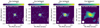 |
Fig. 3. Same as Fig. 1 but for IRC −10529. |
| In the text | |
|
Fig. 4. Same as Fig. 1 but for W Aql. The position of the F9 main sequence companion is indicated by the yellow cross. |
| In the text | |
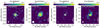 |
Fig. 5. Same as Fig. 1 but for SV Aqr. |
| In the text | |
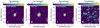 |
Fig. 6. Same as Fig. 1 but for U Del. |
| In the text | |
|
Fig. 7. Similar to Fig. 1 but for π1 Gru. The centre of the secondary peak, corresponding to the C companion, is marked by the black cross on the extended, combined, and UD-subtracted plots. The yellow cross in the middle-left panel indicates the position of the B companion based on Gaia observations. |
| In the text | |
 |
Fig. 8. Same as Fig. 1 but for U Her. |
| In the text | |
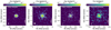 |
Fig. 9. Same as Fig. 1 but for R Hya. |
| In the text | |
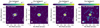 |
Fig. 10. Same as Fig. 1 but for T Mic. |
| In the text | |
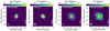 |
Fig. 11. Same as Fig. 1 but for S Pav. |
| In the text | |
 |
Fig. 12. Same as Fig. 1 but for IRC+10011. |
| In the text | |
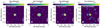 |
Fig. 13. Same as Fig. 1 but for V PsA. |
| In the text | |
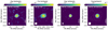 |
Fig. 14. Same as Fig. 1 but for RW Sco. |
| In the text | |
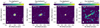 |
Fig. 15. Same as Fig. 1 but for KW Sgr. |
| In the text | |
 |
Fig. 16. Same as Fig. 1 but for VX Sgr. |
| In the text | |
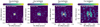 |
Fig. 17. Same as Fig. 1 but for AH Sco. |
| In the text | |
|
Fig. 18. DoLP around T Mic observed with SPHERE (from Montargès et al. 2023) with the UD-subtracted contours observed with ALMA plotted in white (see Fig. 10). The position of the AGB star is indicated by the green cross. |
| In the text | |
|
Fig. 19. Examples of spectral index determinations for W Aql (left) and U Her (right) computed from the combined Band 6 data. The spectral index (colours) is shown for the pixels where it is well-defined. The dashed green circle indicates the area, centred on the continuum peak, equal to the beam size convolved with the UD radius. Black contours indicate the combined continuum (see Figs. 4 and 8). Similar plots for the remaining ATOMIUM sources are given in Fig. B.5. |
| In the text | |
|
Fig. 20. Comparison between measured NIR and calculated stellar radii (left) and between the NIR and ALMA UD diameters (right). In each case, the dotted line represents a 1:1 relation. The dashed line in the right panel represents a fit to the measured AGB data points using orthogonal distance regression (Eq. (4)), with the grey region the uncertainty on this fit. The dot-dashed brown line shows the best linear fit for a relation forced to pass through the origin. See text for details. The shaded region in the right panel shows the uncertainty on the fit. The shaded region in the left panel shows that the measured NIR radii and the calculated radii for most stars fall within 15% of a 1:1 relation. |
| In the text | |
|
Fig. 21. Monochromatic luminosities plotted against physical sizes, as calculated from the UD fits. Left: All the stars. Right: Stars within the dashed rectangle in the left panel. The error bars are omitted in this panel for clarity. The dotted vertical line is plotted at a radius of 2.95 × 1013 cm and separates the SR AGB stars from the Mira variables, as does the dotted horizontal line plotted at 1.2 × 10⁷ mJy pc2. |
| In the text | |
|
Fig. 22. UD radii (left) and monochromatic fluxes (right) plotted against the pulsation period. The dashed black line in the left panel is a fit to the Mira variables. The dotted brown line in the right panel is a fit to the RSGs and the two Mira variables IRC−10529 and IRC+10011. |
| In the text | |
|
Fig. 23. DoLP around π1 Gru observed with SPHERE (from Montargès et al. 2023) with the combined continuum contours observed with ALMA plotted in white (see Fig. 7), showing good agreement. The position of the AGB star is indicated by the large red cross, and that of the C companion by the smaller yellow cross. |
| In the text | |
|
Fig. 24. DoLP around SV Aqr observed with SPHERE (from Montargès et al. 2023) with the extended continuum contours observed with ALMA plotted in white (see Fig. 5). The position of the AGB star is indicated by the green cross. |
| In the text | |
|
Fig. 25. DoLP around KW Sgr observed with SPHERE (from Montargès et al. 2023) with the UD-subtracted contours (at 3 and 5σ) observed with ALMA plotted in white (see Fig. 15). The emission from the two telescopes is in good agreement. The position of the AGB star is indicated by the green cross. |
| In the text | |
|
Fig. 26. Mass-loss rates plotted against physical sizes (left), as calculated from the UD fits, and monochromatic luminosities (right), for the AGB stars. The vertical error bars indicate assumed 50% uncertainties on the mass-loss rates. |
| In the text | |
Current usage metrics show cumulative count of Article Views (full-text article views including HTML views, PDF and ePub downloads, according to the available data) and Abstracts Views on Vision4Press platform.
Data correspond to usage on the plateform after 2015. The current usage metrics is available 48-96 hours after online publication and is updated daily on week days.
Initial download of the metrics may take a while.