| Issue |
A&A
Volume 704, December 2025
|
|
|---|---|---|
| Article Number | A68 | |
| Number of page(s) | 21 | |
| Section | Stellar structure and evolution | |
| DOI | https://doi.org/10.1051/0004-6361/202555349 | |
| Published online | 01 December 2025 | |
Far beyond the Sun
III. The magnetic cycle of ι Horologii
1
Leibniz Institute for Astrophysics Potsdam, An der Sternwarte 16, 14482 Potsdam, Germany
2
European Space Agency, ESTEC, Keplerlan 1, 2201 AZ Noordwijk, The Netherlands
3
School of Earth and Space Sciences, Peking University, Beijing 100781, China
4
Universität Potsdam, Institut für Physik und Astronomie, Karl-Liebknecht-Straße 24/25, 14476 Potsdam-Golm, Germany
5
Université Paris-Saclay, Université Paris Cité, CEA, CNRS, AIM, 91191 Gif-sur-Yvette, France
6
CNRS-IRAP, 14, avenue Edouard Belin, F-31400 Toulouse, France
7
Eberhard Karls Universität, Institut für Astronomie und Astrophysik, Sand 1, 72076 Tübingen, Germany
8
Centro de Astrobiología (CSIC-INTA), ESAC Campus, Camino Bajo del Castillo, E-28692 Villanueva de la Cañada, Madrid, Spain
⋆ Corresponding author: This email address is being protected from spambots. You need JavaScript enabled to view it.
Received:
30
April
2025
Accepted:
29
September
2025
Abstract
We present a comprehensive investigation of the magnetic cycle of the young, active solar analog ι Horologii based on intensive spectropolarimetric monitoring with HARPSpol. Over a nearly three-year campaign, the technique of Zeeman-Doppler imaging was used to reconstruct 18 maps of the large-scale surface magnetic field of the star. These maps trace the evolution of the magnetic field morphology over approximately 139 stellar rotations. Our analysis uncovers a pronounced temporal evolution, including multiple polarity reversals and changes in the field strength and geometry. We examined the evolution of the poloidal and toroidal field components, finding that the toroidal component varies strongly in concert with the chromospheric activity. Furthermore, for the first time, we reconstructed stellar magnetic butterfly diagrams, which we used to trace the migration of large-scale magnetic features across the stellar surface, determining a magnetic polarity reversal timescale of roughly 100 rotations (∼773 d). In addition, by tracking the field-weighted latitudinal positions, we obtained the first estimates of the large-scale flow properties on a star other than the Sun, identifying possible poleward and equatorward drift speeds for different field polarities. These results provide critical insights into the dynamo processes operating in young solar-type stars and enable a direct comparison with the solar magnetic cycle.
Key words: techniques: polarimetric / stars: activity / stars: magnetic field / stars: individual: ι Horologii / stars: individual: HD 17051 / stars: solar-type
© The Authors 2025
 Open Access article, published by EDP Sciences, under the terms of the Creative Commons Attribution License (https://creativecommons.org/licenses/by/4.0), which permits unrestricted use, distribution, and reproduction in any medium, provided the original work is properly cited.
This article is published in open access under the Subscribe to Open model. This email address is being protected from spambots. You need JavaScript enabled to view it. to support open access publication.
1. Introduction
Over the past 25 years, the study of magnetic fields in late-type stars has benefited from improvements in both instrumentation and observational methods. Data from high-resolution spectropolarimeters such as NARVAL (Aurière 2003), ESPaDOnS (Donati et al. 2003), PEPSI (Hofmann et al. 2002; Strassmeier et al. 2015), and HARPSpol (Piskunov et al. 2011), analyzed with procedures like least-squares deconvolution (LSD; Donati et al. 1997; Kochukhov et al. 2010) and single-value decomposition (Carroll et al. 2012), have been used with remarkable success to detect the very weak polarization signatures induced by magnetic fields via the Zeeman effect (Donati & Landstreet 2009; Reiners 2012). Furthermore, the technique of Zeeman-Doppler imaging (ZDI; Semel 1989; Donati & Brown 1997; Piskunov & Kochukhov 2002; Kochukhov & Piskunov 2002) has provided a way to reconstruct the spatial distribution of large-scale surface magnetic fields in stars of various spectral types (see Donati et al. 2011; Kochukhov et al. 2017).
The aforementioned spectropolarimetric observations require a significant amount of telescope time, limiting current survey-scale efforts to magnetic field detections alone (Marsden et al. 2014; Mengel et al. 2017). Still, ZDI snapshots exist for a growing number of stars (e.g., Petit et al. 2008; Fares et al. 2013; Do Nascimento et al. 2016), with some systems having their large-scale fields mapped over multiple epochs, typically on yearly timescales (e.g., Morin et al. 2008, 2010; Fares et al. 2010, 2012). These ZDI monitoring studies have revealed a variety of temporal behaviors of the large-scale field across spectral types. In the case of Sun-like stars, some objects display field strength variability without changes in polarity in the observed time span (Tobs). Examples include HD 141943, (G0IV, Tobs ∼ 4 yr; Marsden et al. 2011), HN Peg (G0V, Tobs ∼ 6 yr; Boro Saikia et al. 2015), and EK Dra (G1.5V, Tobs ∼ 5.5 yr; Waite et al. 2017). In other cases, single polarity reversals in one or more components of the large-scale magnetic field have been observed. Stars in this group include HD 78366 (G0V, Tobs ∼ 3.0 yr; Morgenthaler et al. 2011), ξ Boo A (G7V, Tobs ∼ 3.5 yr; Morgenthaler et al. 2012), HD 29615 (G3V, Tobs ∼ 3.5 yr; Hackman et al. 2016), HD 75332 (F7V, Tobs ∼ 12 yr; Brown et al. 2021), and LQ Hya (K1V, Tobs ∼ 6.0 yr; Lehtinen et al. 2022), among others (see Bellotti et al. 2025).
So far stellar magnetic cycles, understood as a double (or more) polarity reversals in the temporal large-scale magnetic evolution, have been found using ZDI in the following objects: τ Boo (F7V, Tobs ∼ 8.5 yr; Donati et al. 2008; Fares et al. 2009, 2013; Mengel et al. 2016), ϵ Eri (K2V, Tobs ∼ 10 yr; Jeffers et al. 2014, 2017, 2022), 61 Cyg A (K5V, Tobs ∼ 11 yr; Boro Saikia et al. 2016, 2018a), χ1 Ori (G0V, Tobs ∼ 10 yr; Rosén et al. 2016; Willamo et al. 2022), κ Ceti (G5V, Tobs ∼ 10 yr; Boro Saikia et al. 2022), HD 9986 (G5V, Tobs ∼ 15 yr; Bellotti et al. 2025), and HD 56124 (G0V, Tobs ∼ 13 yr; Bellotti et al. 2025). The long baseline of spectropolarimetric observations has allowed us to start connecting the properties of these ZDI magnetic cycles with previously published stellar activity cycles (See et al. 2016). The latter are typically detected in magnetic proxies such as the chromospheric Ca II H&K S-index from Mount Wilson (e.g., Baliunas et al. 1995; Hall et al. 2007, 2009), the coronal behavior in X-rays (see Wargelin et al. 2017 and references therein), and, in a very few cases, via simultaneous activity diagnostics from the photosphere to the corona (Amazo-Gómez et al. 2023).
Despite this progress, it is clear that ZDI monitoring of additional systems is required to improve our understanding of magnetic and activity cycles in cool stars. This is one of the objectives of the Far Beyond the Sun campaign, through which we conducted an unprecedented intensive spectropolarimetric monitoring of the young Sun-like star ι Horologii (G0V, age ∼600 Myr; Vauclair et al. 2008; Bruntt et al. 2010). As discussed in the first papers of this series, ι Hor is the youngest and most active planet-hosting star with reported cyclic chromospheric and coronal activity behavior (Metcalfe et al. 2010; Alvarado-Gómez et al. 2018). The star also displays one of the shortest and best-sampled X-ray cycles to date ( yr; Sanz-Forcada et al. 2013, 2019), making it an exceptional target to follow up on over its short cycle.
In this paper we present 18 separate ZDI large-scale magnetic field maps of ι Hor spanning nearly three years, sufficient to cover two complete coronal cycles and resolve the magnetic cycle. Details on the observations and ZDI reconstructions are presented in Sect. 2. Results and analysis are included in Sect. 3. We discuss and summarize our findings in Sects. 4 and 5.
2. Observations
The observations in this project were acquired using the spectropolarimetric mode of the HARPS spectrograph (HARPSpol), mounted on the ESO 3.6 m telescope at the La Silla Observatory in Chile (Mayor et al. 2003; Piskunov et al. 2011). We obtained circularly polarized spectra (Stokes V) of ι Hor on 199 separate nights over the course of six consecutive ESO observing periods (96 to 101). As described in Alvarado-Gómez et al. (2018), two-week1 epochs were scheduled three times per semester, yielding a total of 18 separate visits with sufficient rotational phase coverage for individual ZDI reconstructions.
2.1. Data reduction
The data processing was described in detail in Alvarado-Gómez et al. (2018) and is briefly summarized here. The circularly polarized (Stokes V) and diagnostic null (N) spectra were derived by combining consecutive exposures (each one consisting of four sub-exposures matching orthogonal polarization angles) using the ratio method (see Donati et al. 1997; Bagnulo et al. 2009 for details). Between two and three consecutive Stokes V exposures were acquired each night, with a combined integration time of approximately 1 h.
The observations were reduced employing the HARPSpol-compatible version of the LIBRE-ESPRIT pipeline (Donati et al. 1997), which applies standard spectroscopic corrections (e.g., bias subtraction, flat-fielding, masking bad pixels, cosmic ray removal), wavelength calibration (using two reference ThAr arc spectra per night), and the polarization calculation and subtraction of continuum polarization. As was shown in Amazo-Gómez et al. (2023), this procedure retains the nominal RV precision of the HARPS spectrograph (see also Hébrard et al. 2016; Hussain et al. 2016; Alvarado-Gómez et al. 2018). A two-step continuum normalization was carried out, using first HARPS settings (R ∼ 115 000) for the automatic procedure included in the ISPEC package (Blanco-Cuaresma et al. 2014), and then performing a manual fitting of cubic-splines over 15 nm windows throughout the entire spectral range (378 − 691 nm). The reduced data products consisted of unpolarized intensity profiles (Stokes I), circularly polarized spectra (Stokes V), and diagnostic null profiles (N), which are used to check for instrumental noise and artifacts.
In moderately active solar-type stars such as ι Hor, the detection of surface magnetic features via Zeeman splitting using individual spectral lines is currently unfeasible (see Donati & Landstreet 2009; Reiners 2012). In order to maximize the information contained in thousands of photospheric individual line profiles, we employed the multiline technique of LSD (Donati et al. 1997; Kochukhov et al. 2010). Commonly used in ZDI studies, this cross-correlation technique adds coherently the polarimetric signal from multiple lines, yielding mean profiles per observation (LSD Stokes I, V, and N) with very high signal-to-noise ratios (S/N).
A photospheric line list, with information on rest wavelengths, line depths, and Landé factors, is required to perform the LSD procedure. The Vienna Atomic Line Database (VALD32; Kupka et al. 2000; Ryabchikova et al. 2015), was used for this purpose using the stellar properties reported by Bruntt et al. (2010), and imposing a line-depth detection threshold of 0.05 (in normalized units). The original photospheric model (∼9500 spectral lines in the HARPS wavelength range) was improved following the procedure discussed in Alvarado-Gómez et al. (2015), tailoring all the line depths to an observed spectrum of the star, and removing spectral lines that largely deviate from the self-similarity condition required by LSD. The final line list for ι Hor has 8834 entries and served to retrieve LSD profiles over the velocity range between −5.0 km s−1 and 45.4 km s−1, with a velocity step of Δv = 0.8 km s−1, closely matching the HARPS detectors’ pixel width.
2.2. Mapping the large-scale magnetic field: Zeeman-Doppler imaging
As mentioned earlier, we used ZDI to map the large-scale surface magnetic field of ι Hor for each observing run during the ∼3-year campaign. ZDI is an indirect imaging technique that inverts time series of spectropolarimetric observations to reconstruct the photospheric magnetic field in a two-dimensional projection. Our analysis uses circularly polarized profiles, which are only sensitive to the line-of-sight component of the stellar magnetic field and therefore subject to cancellation effects in the presence of complex multipolar small-scale fields. The resulting maps can therefore only reconstruct the large-scale component of the residual surface magnetic field (see, e.g., Reiners 2012; Lehmann et al. 2019). As in other image inversion methods, a regularization procedure (such as maximum smoothness or minimum information), is imposed on the reconstruction to ensure the uniqueness of the solution (see Semel 1989; Brown et al. 1991; Hussain et al. 2000; Piskunov & Kochukhov 2002; Carroll et al. 2012). The maps are regularized using maximum entropy (Skilling & Bryan 1984), fitting the spectropolarimetric datasets up to an optimal reduced chi-square (χR2) value given by the entropy-growth stopping criterion introduced by Alvarado-Gómez et al. (2015).
The technique of ZDI can be used to further refine several of the key stellar parameters and spectral line properties of ι Hor reported by Alvarado-Gómez et al. (2018) (and references therein). Parameters such as rotation period, vsin(i), and inclination angle are fine-tuned by allowing them to vary over the ranges reported in the literature and minimizing the χR2-fit to the data (e.g., Jeffers & Donati 2008; Waite et al. 2015). Using this approach we find vsin(i) = 6.3 km s−1 and a rotation period Prot = 7.73 d; both are consistent with previous estimates and with values derived from our photometric analysis in Amazo-Gómez et al. (2023). Given the published radius of 1.16 R⊙, this corresponds to an inclination angle of ∼56°. The following results were obtained assuming an inclination angle of 60°. The magnetic field maps presented here employ the ZDI code first described in Hussain et al. (2002), which has since been updated to implement a spherical harmonic description of the large-scale magnetic field (see Lehmann et al. 2021) and briefly summarized again here. Essentially, the surface field vector is decomposed as the sum of poloidal (potential, α and β) and toroidal (non-potential, γ) components, which are expressed in terms of spherical-harmonics: Equations 1-4 from Lehmann et al. (2021) are reproduced here for completeness.
The vector magnetic field B is described in terms of its constituent radial, azimuthal and meridional field components (Br, Bϕ, Bθ), following Elsasser (1946) and Appendix III of Chandrasekhar (1961), but applying a left-handed coordinate system,
 (1)
(1)
 (2)
(2)
 (3)
(3)
so that (Br, Bϕ, Bθ) = B, where Pℓm ≡ cℓmPℓm(cos θ) are the associated Legendre polynomial of mode ℓ and order m and cℓm is a normalization constant:
 (4)
(4)
In the left-handed coordinate system, the radial Br component points radially outward, the azimuthal component Bϕ runs in the clockwise direction (as viewed from the north pole), and the meridional component Bθ runs with colatitude from north to south. In the (r, ϕ, θ) spherical harmonic system used here, the αℓm and βℓm components describe the poloidal field whereas the γℓm components describe the toroidal field (also see Lehmann et al. 2021).
By using spherical harmonics to describe the mapped magnetic field, it is relatively simple to reconstruct and examine the large-scale magnetic field on different length scales. An important first step in reconstructing the magnetic field morphology of stellar surfaces is to identify the smallest length scale to which the spectral time series are sensitive – this is largely a function of v sin i of the star, the instrumental resolution, the intrinsic line profile width, phase coverage, and the exposure time of the observations (Kochukhov 2016). For ι Hor, we find that allowing modes beyond ℓ = 7 does not yield additional information; all the reconstructions presented here are hence restricted to ℓmax = 7, corresponding well to the ∼25° resolution at the equator and closely matching the optimal spatial resolution allowed due to ι Hor’s v sin i.
During the reconstruction it is also possible to apply higher weights or penalties to even or odd ℓ modes, thus favouring antisymmetric or symmetric large-scale fields, respectively. In this study, we produced three sets of solutions for each epoch: unconstrained (i.e., in which all modes are allowed and no weighting is applied), symmetric, and antisymmetric. This enabled an evaluation of how robust the large-scale field reconstructions are. In addition, we learned whether an antisymmetric or symmetric description better applies to ι Hor based on a comparison of the information content of each set of maps.
The large-scale field can be characterized in terms of several key properties, for example polarity reversal, axisymmetry, the evolution of the magnetic field strength, and the size of the mean B2 (proportional to the magnetic energy). We examined the evolution of these characteristics over time and their relation to the chromospheric activity indicators analyzed in Papers I and II. In addition, we evaluated the cycle variability of the dipole, quadrupole, and octupole components (i.e., ℓ = 1 − 3) of the toroidal and poloidal large-scale magnetic field.
3. Results and analysis
The full set of the large-scale ZDI magnetic field maps reconstructed consistently and using the same entropy-growth stopping criterion are shown in Figs. 1 to 3. These maps show the solutions for unconstrained ℓ-modes (i.e., not favouring an antisymmetric or symmetric large-scale field description). From a visual inspection of the maps, it is clear that the magnetic field evolves significantly over the course of the ∼3 year time-span (approximately 1077 d, which correspond to ∼139 stellar rotations, assuming Prot = 7.73 d).
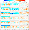 |
Fig. 1. Unconstrained ZDI reconstruction of the large-scale magnetic field maps of ι Hor in latitude-longitude equi-rectangular projection. Columns contain the radial (BR, left), azimuthal (BA, middle), and meridional (BM, right) field components, with the color scale indicating the magnitude (in gauss) and field polarity in each case. Each row corresponds to a different observing epoch, as indicated (Epochs 1 to 6), with the observed phases denoted by black tick marks in longitude (upper x-axes). The campaign day and number of stellar rotations (measured from BJD = 2457300.78580 to the first night of observations of a given epoch) are listed on each map. The segmented line shows the visibility limit imposed by the inclination of the star (i = 60 deg). |
An epoch by epoch description of the evolution of the stellar large-scale magnetic field of ι Hor can be found in the Appendix A. As illustrated in Fig. 1, the field is initially characterized by a dominant radial component (BR) with strengths ranging roughly from −6.4 G to 5.1 G, accompanied by a significant negative azimuthal component (BA) and a weaker meridional field (BM). As the campaign progresses, notable changes occur: the field strength increases in some epochs (with |BR| and |BA| reaching up to approximately 12 G and 16 G, respectively), and the geometry of the field evolves. Several epochs show distinct polarity reversals in both BR and BA, for example Epochs 8 (Fig. 2) and 14 (Fig. 3), with multiple reversals throughout, suggesting the re-initiation of the magnetic cycle. The azimuthal field, in particular, transitions from a broad negative band to configurations featuring mix-polarity regions, with the mid-latitude bands either emerging or disappearing across the epochs.
A sample of the Stokes V time series used to derive these maps are shown in Fig. 4 (Epochs 1 − 5), with the remaining ones presented in Figs. B.1–B.3. We also include the null (N) spectra, which we used to check for instrumental contributions to the polarization signature. As demonstrated in these spectral time-series, strong Zeeman signatures are detected at all observed epochs, with the amplitude and morphology of the Zeeman signatures varying over timescales on the order of one night. Throughout the campaign, the ZDI reconstructions consistently achieve good fits to the observed Stokes V LSD profiles, with χR2 values typically near 1.0. Still, some epochs exhibit higher values that could be in part due to variations in the magnetic field within epochs, as well as observational phase gaps and worse S/N (which can affect the location of the optimal χR2 value; see Alvarado-Gómez et al. 2015). Nevertheless, the Stokes V time-series alone indicate changing, complex multipolar surface fields, which are further confirmed in the resulting ZDI magnetic field maps.
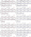 |
Fig. 4. Recovered LSD profiles from the spectropolarimetric observations of ι Hor. Each row contains a different observing epoch (Epochs 1 to 5), with individual observing phases (Φ) shown in each subpanel. Left column: ZDI fits (red) to the circularly polarized data (Stokes V, black), with the optimal reduced χR2 achieved in each case. Right column: Corresponding diagnostic null (N) spectra. Both profiles have been enhanced (by a factor of 5.0 × 10³) and normalized to the continuum intensity (IC) for visualization purposes. The ZDI fits to the remaining epochs (6 to 18) are presented in Figs. B.1–B.3. |
As the ZDI reconstructions shown in Figs. 1–3 were performed in an unconstrained manner, this led to no magnetic field being recovered below −60° latitude, due to the star’s inclination angle. To complete the “missing” field in the obscured hemisphere (assumed here to correspond to southern latitudes), we can drive the solutions to antisymmetric and symmetric distributions consistent with the data by weighting against odd and even modes, respectively. We show the corresponding symmetric and antisymmetric maps in Appendix C. We find that ι Hor tends to host an antisymmetric large-scale field, as the maps derived from the unconstrained solutions have more power in the even spherical harmonic modes and tend to resemble the antisymmetric maps.
Finally, note that the meridional field maps are more subject to cross-talk – this is a well-known limitation that arises from the relatively weak contribution from this component to the circularly polarized Stokes V profiles in high inclination stars (see Donati & Brown 1997; Kochukhov & Piskunov 2002). Reconstructions based on time series of all Stokes V, Q, and U profiles would help address this limitation, but Stokes Q and U signatures are typically an order of magnitude weaker in cool stars compared to Stokes V (e.g., Rosén et al. 2015; Waite et al. 2015) and, hence, the exposure times required would be too long to derive maps with high cadence employing all four Stokes profiles. As such, in the following sections, we mainly focus on the properties of the radial and azimuthal components of the large-scale field.
3.1. The large-scale magnetic field of ι Hor: Global properties
Figure 5 traces how the ratio of the poloidal to toroidal field changes over the different epochs covered in this study. There appears to be a dependence on chromospheric activity in the recovered total magnetic field. By comparing the middle and lower panels of Fig. 5, we see that the large-scale toroidal field changes more dramatically than the poloidal field in terms of both strength and axisymmetry. The poloidal field component stays predominantly non-axisymmetric, with only three epochs corresponding to an axisymmetry of 50% or greater (see Table 1). On the other hand, the toroidal field component undergoes much larger changes in axisymmetry, reaching over 80% in half the epochs; the epochs at which it is stronger and more axisymmetric appear closer in time to chromospheric activity maxima, while the minima are generally associated with weaker and non-axisymmetric toroidal fields.
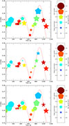 |
Fig. 5. Evolving global magnetic field properties for ι Hor plotted as a function of the chromospheric S-index and time. Top: Axisymmetry and log Btot2 for the total field. Middle and bottom: Axisymmetry and log B2 for the poloidal field and toroidal field components, respectively. The solid red line shows the best two-period model fit to Ca II H&K observations from Amazo-Gómez et al. (2023). Day “0” corresponds to BJD = 2457300.78580. The symbol sizes scale with log B2, and symbols for poloidal- and toroidal-dominated fields range from red to blue. The degree of non-axisymmetry is represented by symbol shapes, ranging from circular for a fully axisymmetric field and star-shaped symbols for non-axisymmetry. |
Properties of the large-scale magnetic field of ι Hor obtained from the ZDI reconstructions.
Our dense time-sampling allows a detailed analysis of how different properties of the large-scale field evolve with activity cycle. It also allows a comparison with a similar analysis of the solar cycle conducted by Lehmann et al. (2021), who identified which features of the large-scale field morphology could be recovered using ZDI techniques. They applied ZDI to magnetograms based on solar cycle 23 and found that, while the size of the large-scale field tended to be underestimated in ZDI maps, changes in both axisymmetry and toroidal field could be used to detect and follow the solar cycle. They also observed that the strongest tracer of the solar activity cycle was the axisymmetric field; with the fraction of axisymmetry decreasing essentially linearly with increasing S-index (see Lehmann et al. 2021, Fig. 8). Hackman et al. (2024) used a similar approach, applying ZDI to simulated data based on dynamo models tracing different activity levels; they similarly find that while weaker magnetic field strengths are poorly recovered, there is a sensitivity to the relative amounts of toroidal and poloidal field. On ι Hor, we find no clear trend in the fraction of axisymmetry with S-index; though the total field reconstructed tends to be more axisymmetric during peaks of the chromospheric activity cycle, albeit with quite some scatter.
On the Sun, another tracer of the activity cycle is the fraction of the toroidal field, with ftor in dipolar, quadrupolar and octupolar components all following the activity level of the Sun. On ι Hor, the octupolar field component (ftor) shows no trend with the activity cycle, but the ftor in the dipolar and quadrupolar components weakly trace the activity levels. An analysis of the time evolution of the real component of the large-scale field (α, β, γ) also reveals a possible trend with γℓ = 1, 2, which traces the dipolar and quadrupolar components of the toroidal field.
The toroidal component of the magnetic energy, ⟨Btotal2⟩, which traces the peaks of the chromospheric cyclic activity, increases (see Fig. 5). However, albeit with significant scatter, the strongest tracers of the chromospheric activity of ι Hor are the axisymmetric total energy ⟨Baxi2⟩, and the energy of its toroidal and toroidal axisymmetric component (⟨Btor, axi2⟩; see Fig. 6). We find Spearman correlation coefficients of 0.59 for the axisymmetric magnetic energy versus the S-index evolution (given by the two-period fit) and 0.54 for the axisymmetric toroidal field energy versus the S-index fit. Their standard t-test significance p-values are 0.01 (S-index vs. ⟨Baxi2⟩) and 0.02 (S-index vs. ⟨Baxi, tor2⟩), which respectively indicate a weak and moderate correlation between the involved quantities. We assessed the significance of these correlations by calculating p-values after a two-sided permutation test, finding similar results. This behavior is drastically different from the Sun (see Fig. C2 in Lehmann et al. 2021), where the non-axisymmetric energy ⟨Bnaxi2⟩ is the stronger tracer of the underlying magnetic cycle.
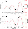 |
Fig. 6. Similar to Fig. 5 but showing the evolution of the axisymmetric total energy, ⟨Baxi2⟩, and axisymmetric toroidal energy, ⟨Btor, axi2⟩, that most closely follow the evolution in the chromospheric activity (traced by the Ca II H&K S-index; dashed red line). |
3.2. Stellar butterfly diagrams
Based on the 18 different ZDI reconstructions of ι Hor (Figs. 1 to 3) we can retrieve a counterpart of the well-known solar magnetic butterfly diagrams (e.g., Hathaway 2015; Cameron et al. 2018). For each ZDI reconstruction, we considered 10° latitudinal strips3 over which longitudinally averaged values of the radial and azimuthal magnetic field components are extracted. Since the averaging procedure is performed over the signed magnetic field, the resulting “meridional4 snapshots” (covering the dates comprising each ZDI epoch) capture the dominant field polarity at different latitudes. By plotting all the retrieved snapshots as a function of time, we could construct the butterfly diagrams of ι Hor for BR and BA, which are presented in Fig. 7. We also include the corresponding number of stellar rotations since the beginning of the campaign (with Prot = 7.73 d), as well as the two-period fit to the Ca II H&K S-index variations characterizing the evolution of the chromospheric activity (Amazo-Gómez et al. 2023).
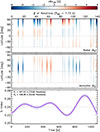 |
Fig. 7. Top and middle: Butterfly diagrams of the radial (top) and azimuthal (middle) large-scale magnetic field of ι Hor. These synoptic maps display the longitudinally averaged magnetic field strength (color bar, in gauss), extracted over 10° latitudinal strips on the individual ZDI epochs (Figs. 1 to 3). Bottom: Best two-period fit to the Ca II H&K S-index variations obtained by Amazo-Gómez et al. (2023). The shaded region encapsulates the 1σ period and amplitude uncertainties. Day “0” corresponds to BJD = 2457300.78580 (2015-10-05 06:51:33.12 UTC), and a secondary x-axis indicates the number of stellar rotations covered by the campaign (assuming Prot = 7.73 d). |
Notice that the width of each snapshot (i.e., vertical slices) in the diagram is not the same among the various epochs, illustrating the number of consecutive rotations used for retrieving each ZDI map. While ZDI studies commonly achieve better phase coverage by combining data from multiple rotations (even nonconsecutive ones), it is clear that this would clearly impact the capability to reconstruct a butterfly diagram. Ideally, each ZDI map should be recovered over a single rotation, minimizing in this way the evolution the field can have in between epochs. As such, wider snapshots in Fig. 7 indicate epochs with more uncertainty in terms of the long-term magnetic field evolution.
As expected from the individual ZDI maps, multiple polarity reversals of both components of the large-scale field of ι Hor are evident in Fig. 7. Around the visible pole, BR flips sign two times (between rotations 48.64 – 56.51 and 99.46 – 104.76) while, closer to the equator, three polarity reversals are seen in BA (between rotations 17.56 – 33.91, 62.58 – 82.03, and 128.35 – 133.00). At face value, the large-scale magnetic field does not show an immediate correspondence with the double periodicity observed in the chromospheric activity of the star. However, the magnetic field evolution appears to be more regular compared to the Ca II H&K S-index. To better quantify the magnetic cycle timescales, we analyzed the temporal evolution of the longitudinally averaged magnetic field components at different locations on the stellar surface.
Figure 8 shows temporal profiles for  and
and  , extracted at four different 10° latitude strips including the visible pole (90°) and the stellar Equator (0°). The error bars indicate the absolute variation (standard deviation5) of each component with longitude and within the corresponding latitudinal bin. To determine the periodicity at each latitudinal band, we considered a single-period sinusoidal model,
  composed of three free parameters – amplitude (B0), period (PB = 2π/ωB), and normalized phase (ϕB) – and found the best-fit to the individual temporal profiles of
  and
and  (solid lines in Fig. 8). Similar fits were obtained for all the other latitude bins down to the visibility limit (−60°). The resulting model parameters with their formal uncertainties are listed in Table 2.
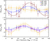 |
Fig. 8. Temporal profiles of the longitudinally averaged radial (top) and azimuthal (bottom) large-scale magnetic field of ι Hor. Symbols and colors denote the range of latitudes of extraction, with error bars indicating the standard deviation of each component within the associated latitude strip as well as with longitude. Solid lines (with corresponding colors) show the resulting best-fit solution for a single-period model (three free parameters) at a given latitude bin (see text for details). |
Several aspects of Fig. 8 and Table 2 are noteworthy. First of all, both field components reveal a timescale of approximately 100 rotations for the completion of the magnetic cycle (consistent with the evolution observed in the ZDI maps and in Fig. 7). There are however some deviations in the determined polarity reversal timescale, with larger values (by up to ∼60%) identified in  and smaller ones (by ∼20%) in the evolution of
  . In the case of the radial component, these deviations appear at mid-latitudes (20° – 40°) in both hemispheres (see Table 2). For instance, evolution at 30° (Fig. 8, top panel, orange) displays an associated reversal timescale of 147.2 ± 24.8 rotations (∼1137.9 d), whereas a value of 154.5 ± 14.9 rotations (∼1194.3 d) emerges at −30°. Note that these longer polarity reversal timescales exceed our observational window of ∼139 rotations (∼1077.0 d), which is reflected by their relatively large uncertainties (∼20%) even when the field variance in the individual epochs is small. In terms of the amplitude of variability, there is a clear trend of decreasing
  with latitude, starting with a maximum value close to 7.5 G for the visible pole, down to sub-gauss amplitudes at the stellar equator and in the partially obscured hemisphere. With the exception of latitude 40° (which displays the largest uncertainty in the period determination), the magnetic cycle phase in
  does not show too much variation staying within the 0.4 − 0.6 range for all latitudes.
Best-fit parameters of the single-period sinusoidal models describing the evolution of the magnetic cycle in ι Hor.
The situation is slightly different for the azimuthal component (Table 2, Fig. 8, bottom panel). The majority of latitudes display  values of around 90 rotations, with 80.9 ± 7.7 rotations (∼622.9 d) at −30° the shortest timescale for a polarity reversal in this component. While some longer values (≳105 rotations) emerge at high latitudes (70°–90°) and at −20°, these are the most uncertain in terms of both
  (up to ∼20%) and
  (up to ∼50%). The cycle amplitude in this component shows a maximum value of
  G around 30°, declining in strength down to sub-gauss levels at very high latitudes (80°–90°) as well as in the obscured hemisphere (≤ − 20°). As evidenced by the best-fit curves plotted in Fig. 8, there is a small phase difference between the radial and azimuthal large-scale magnetic field at the latitudes that show the largest cycle amplitudes (i.e., at 90° −60° for
  and 30° −0° for
  ). From the best-fit parameters presented in Table 2, this phase difference is on the order of 0.1, which corresponds to ∼10 rotations (77.3 d) assuming a mean cycle period of ∼100 rotations for both components.
3.3. Large-scale flows
Apart from the analysis of the magnetic cycle period, we could use the butterfly diagrams to put constraints on the large-scale photospheric flows on ι Hor. To our knowledge, this is the first time such an estimate has been carried out on a star different from the Sun.
From each butterfly diagram, we traced the average position of the magnetic regions of a given polarity as a function of time. The calculation was performed on each hemisphere and separately for  and
and  . The extracted pairs of positions-times (rotations) were then fitted by a simple linear function to estimate the speed of the large-scale flow on each field component. This methodology is inspired by similar analyses performed on solar data to retrieve the so-called rush-to-the-poles and equatorward flux migration of the solar magnetic field (e.g., Li et al. 2001; Švanda et al. 2007; Mordvinov et al. 2022). From the behavior observed in the Butterfly diagrams, the analysis that follows assumes that the poleward flux transport dominates the evolution of the radial field, whereas the equatorward drift manifests more strongly in the azimuthal component, being the precursor of spot and facula. Note that while the two components are treated in a similar manner, only the poleward motion is expected to trace the stellar meridional circulation (Choudhuri 2021; Hotta et al. 2023) whereas the equatorward drift would be the result of consecutive emerging magnetic regions as the cycle progresses (Waldmeier 1955; Hathaway 2011).
The results are shown in Fig. 9 for the radial (top) and azimuthal (bottom) components. The individual points show the field-weighted mean latitude of a particular polarity of the field at each epoch. Only the visible hemisphere is considered for the radial field, as the remaining region lacked sufficient information for identifying any trends in latitude for this component. As this averaging procedure takes place over the butterfly diagram values (averaged over longitude), we label it  . In principle, the weighting procedure could also incorporate temporal information (i.e., number of rotations), taking into account the widths of the individual ZDI epochs (see Sect. 3.2). However, most of our maps have similar temporal coverage (between ∼1.0 − 1.9 rotations) with only Epoch 4 largely deviating from this range (3.48). As such, we did not include any temporal uncertainty in our analysis.
For the radial magnetic field (Fig. 9, top) two sets of linear fits are employed in the flow analysis. The first one (solid line) considers all the points of a given polarity, from low latitude regions to the pole, before the polarity reversal. The second case (dashed line) considers only 2-3 epochs before and after the polarity reversal at the visible pole. These two cases are selected to obtain two “limits” on the poleward flow speed (slope), the latter case being faster than the former. The second approach should be closer to the methodology employed on the Sun based on magnetogram data (see, e.g., Mordvinov et al. 2022 and references therein). The first method, however, allowed us to set the lowest speed compatible with the observed evolution of the radial field in the butterfly diagrams (with the added benefit of having more data points for the fit). In this way, we obtain poleward flow speeds between 19.2 ± 1.2 m s−1 (slow) and 69.2 ± 8.6 m s−1 (fast) for the positive polarity. Similarly, the fits to the negative polarity regions yield limit speeds of 16.9 ± 1.6 m s−1 (slow) and 51.3 ± 11.2 m s−1 (fast).
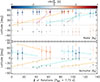 |
Fig. 9. Analysis of the large-scale flows on ι Hor based on the magnetic butterfly diagrams (Fig. 7) for the radial (top) and azimuthal (bottom) components. Individual points indicate the field-weighted mean latitude hosting each polarity at a given epoch, with error bars denoting its standard deviation within the averaged latitudinal bin. Filled colored circles and gray open diamonds indicate locations within the northern and southern hemispheres, respectively. The latitudinally averaged magnetic field strength, |

For completeness, we also consider a two constant-latitude model (i.e., no flow velocity) per polarity (dotted lines in Fig. 9, top panel) to perform a statistical model comparison with the poleward flow models using the Bayesian information criterion (BIC; Schwarz 1978). For the positive polarity, the best-fit zero-slope model yield weighted-mean latitudes of λ1+ = 15.5 ± 5.5° and λ2+ = 80.4 ± 5.3°, with a break at t1 = 52.64 rotations and an associated BIC of 102.8. Similarly, for the negative polarity we obtain λ1− = 23.1 ± 7.3° and λ2− = 70.2 ± 10.9°, with t2 = 102.11 rotations and a BIC value of 94.6. Computing the BIC for the slow poleward linear models (2 free parameters) yields 107.7 and 94.5 for the positive (N = 13 points) and negative (N = 11 points) polarities, respectively. This analysis indicates that the two constant-latitude model is statistically slightly preferred against the slow poleward fit in the positive polarity ( ), whereas the opposite situation occurs for the negative one. However, as mentioned earlier, the slow poleward drift has been taken as a coarse lower limit to the flow speed but admitting a physically motivated preference for the faster speed determined before and after field polarity reversal at the pole (magenta and green fits in Fig. 9). Repeating the two-latitude fit for the 5 points involved in the fast positive polarity6 poleward model yields a BIC value of 42.1, slightly less favored than the corresponding poleward model with a BIC of 41.7. Note that, in general, these results make the two models (poleward flow vs. two-latitude) statistically comparable, so another possible interpretation of the data is that the star has two separate active latitudes. We however stick to the the interpretation based on the meridional flow transport, motivated by the known solar phenomenology and the assumption that the dynamo operating in Sun-like stars like ι Hor should behave similarly as in the Sun.
As can be seen in Fig. 9 (bottom), we consider several “tracks” for fitting the evolution of the azimuthal component. These were constructed by taking all the locations of a given polarity with the requirement of having more than three consecutive epochs and a maximum of one epoch gap per track. This is the reason why some points are not included in the fitting analysis (e.g., negative polarity in the southern hemisphere between rotations 0 − 20 and positive polarity in the northern hemisphere between rotations 100 − 138). Similar to the radial component, the fitted slope yields the mean equatorward drift speed compatible with the observations. In this way, we obtain speed values of 15.1 ± 4.0 m s−1 for the positive polarity and 12.1 ± 3.3 m s−1 for the negative one. These values correspond to the average of the two hemispheres and are based on the three identified tracks for each polarity. Similarly, the average speeds on the northern and southern hemisphere (regardless of the field polarity) yield 13.2 ± 3.3 m s−1 and 14.0 ± 4.1 m s−1, respectively. This suggest that our derived equatorward drift speeds are robust even when employing data from the partially obscured hemisphere. Finally, given that our flow speed and drift rate determinations are inspired by the known solar phenomenology, we replicate in Sect. 4.3 the methodology applied on ι Hor on solar magnetic field observations as a way to assess the performance of our ZDI-based procedure.
4. Discussion
We have presented a comprehensive characterization of the magnetic cycle of the young planet-host Sun-like star ι Hor based on spectropolarimetry and ZDI. In the following subsections we place our results in the context of other cool stars with information on their magnetic cycles as well as with the Sun.
4.1. The large-scale field of ι Hor among cool stars
The Btor2 versus Bpol2 range recovered in the ι Hor maps is similar to what has been observed for solar-type stars with similar ages and rotation periods. In terms of their morphologies, solar-type stars in their first 250 Myr host stronger axisymmetric large-scale fields (Folsom et al. 2016), and as they age (between 250–650 Myr) they show significantly weaker large-scale non-axisymmetric field morphologies that are similar to those found for ι Hor (Folsom et al. 2018). Folsom et al. (2018) note the difficulty of finding trends in magnetic geometry in the 250–650 Myr range and suggest this is due to intrinsic variability as the stars follow longer term cycles. Our maps with dense time sampling of ι Hor’s large-scale field over the course of its cycle further supports this conclusion. As with many of the stars studied in Folsom et al. (2018), ι Hor’s field also tends to have a significant toroidal component for much of its cycle and displays a tendency toward non-axisymmetry.
The dense time-sampling of ι Hor maps presented here also allows a detailed comparison with the solar activity cycle. Lehmann et al. (2021) carried out an analysis of which features of the solar activity cycle would be recovered using ZDI techniques by applying ZDI-like diagnostics to magnetograms acquired during solar cycle 23. While there is a strong trend in the solar activity cycle with the fraction of axisymmetric field recovered; with axisymmetry decreasing essentially linearly with increasing S-index (see Lehmann et al. 2021, Fig. 8), on ι Hor the trend is not as clear. Indeed, the fraction of axisymmetry tends to increase during activity maxima, albeit with quite some scatter. The clearest trends with activity cycle found on ι Hor correspond to Btor2/Bpol2, with both dipolar and quadrupolar components showing increases during the chromospheric activity maxima traced with the chromospheric S-index. Likewise, we see that the axisymmetric total energy ⟨Baxi2⟩, and energy in the toroidal axisymmetric component ⟨Btor, axi2⟩ roughly follow the evolution of the chromospheric activity (with significant scatter).
4.2. Activity and magnetic cycles connection
We can compare the cycle periods obtained for the magnetic field components with the behavior observed in the coronal and chromospheric activity of the star (Sanz-Forcada et al. 2019; Amazo-Gómez et al. 2023). While the X-ray observations indicate a coronal cycle of  yr (∼75.9 rotations), the long-term evolution of the S-index is more consistent with the superposition of two periodicities around
  yr (∼70.7 rotations) and
  yr (∼51.7 rotations). Interestingly, the mean magnetic cycle period of ∼100 rotations would match the solar 2:1 relation (i.e., two activity cycles for one magnetic cycle) with the secondary chromospheric cycle (
 ). While uncertain for the reasons exposed in Sect. 3.2, the second magnetic cycle period in BR (around 150 rotations) would also roughly follow the solar expectation with the coronal (
 ) and the primary chromospheric cycle (
 ). Note also that the ∼20% shorter magnetic cycle period identified in BA is also in agreement with the behavior observed in the solar toroidal magnetic field (Liu & Scherrer 2022).
As with the global magnetic field properties (Sect. 4.1), our results for ι Hor also align well with the activity and magnetic cycle properties established by ZDI studies of other cool stars. Note, however, that none of the previous investigations has been able to resolve the magnetic cycle as we have done for ι Hor (i.e., retrieve a magnetic butterfly diagram), so that comparisons can only be performed on the most general aspects of the cycles.
The studies of Boro Saikia et al. (2016, 2018a) showed that 61 Cyg A displays a Sun-like behavior in its magnetic cycle, where the polarity reversals occur in phase with the observed chromospheric and coronal activity cycle of 7.3 ± 0.1 yr (Baliunas et al. 1995; Robrade et al. 2012). This was the first stellar case in which such a cycle coincidence could be confirmed.
The star ϵ Eri has been found to follow two chromospheric cycles, of 2.95 yr and 12.7 yr (Baliunas et al. 1995; Hatzes et al. 2000; Metcalfe et al. 2013). A coronal counterpart in X-rays to the shorter chromospheric cycle has only recently been confirmed (Coffaro et al. 2020). On the other hand, the ZDI maps obtained by Jeffers et al. (2014, 2017) suggest polarity reversals on timescales that are much shorter than these cycles; two polarity reversals that may be associated with the chromospheric activity minimum have occurred. Thanks to the long term ZDI monitoring efforts, Jeffers et al. (2022) has attempted butterfly diagram reconstructions for this star and for 61 Cyg A but longer and denser monitoring is still required.
The planet-hosting star τ Boo was initially believed to show a 1:3 relation between the magnetic and chromospheric cycle periods (360 vs. 116 days; Baliunas et al. 1997; Henry et al. 2000; Fares et al. 2013). However, more densely sampled ZDI reconstructions discussed by Jeffers et al. (2018) showed polarity reversals in the radial field in phase with the shorter chromospheric cycle (similar to what we observe in ι Hor). Although X-ray observations of the star carried out by Poppenhaeger et al. (2012) found no evidence of such a short coronal activity cycle, a reanalysis of the data performed by Mittag et al. (2017) did find such a periodicity, albeit with a relatively small maximum to minimum amplitude ( ). As such, the authors concluded that τ Boo would also display a solar-like behavior on its activity and magnetic cycles.
Long-term monitoring of κ Ceti’s chromospheric activity showed a high variability exhibiting multiple cycles of 22.3 yr and 5.7 yr (Baliunas et al. 1995; Boro Saikia et al. 2018b). A recent investigation suggests a shorter period of 3.1 yr (Boro Saikia et al. 2022). This short period is suspected to be a harmonic of the 5.7 (6) yr period, but opens the possible scenario of two activity cycles with a 2:1 ratio similar to the Hale and the Schwabe cycles, even though showing a complex temporal evolution, unlike the Sun. The ZDI analysis by Boro Saikia et al. (2022) reports a radial field for κ Ceti with considerable evolution during 6 yr of yearly follow-up. The large-scale magnetic field reconstructions show a polarity reversal of the radial and azimuthal components, with a magnetic cycle period of approximately 10 ± 2 yr.
Finally, ZDI studies of the G dwarfs χ1 Ori (G0V, Prot ≃ 5.0 d), HD 9986 (G5V, Prot ≃ 21.0 d) and HD 56124 (G0V, Prot ≃ 20.7 d) report relatively short magnetic cycle periods – between 3 and 10 yr (Rosén et al. 2016; Willamo et al. 2022; Bellotti et al. 2025) – albeit with significant uncertainties given the sparseness of the ZDI reconstructions. In all cases, however, it does not seem to be a clear connection between the chromospheric S-index variability and the evolution of the large-scale field, with some of these targets originally classified as “variable” by the Mount Wilson survey (Baliunas et al. 1995). From our analysis of ι Hor, it is possible that a denser sampling of the large-scale field is needed to properly capture the behavior and relations between these rapidly evolving cycles.
4.3. Meridional circulation and equatorward drift
As mentioned in Sect. 3.3, there are no estimates of the large-scale photospheric flow properties for stars other than the Sun. Therefore, we compared our ι Hor findings with established solar large-scale flow values, focusing particularly on spatio-temporal speed averages, which should be more directly comparable to those derived from stellar ZDI data.
Including errors, our analysis revealed a poleward flux transport speed within 15 − 78 m s−1 and an equatorward drift in range of 9 − 19 m s−1 for ι Hor. Given the relatively fast activity and magnetic cycles on the star, it is not surprising that these speeds appear larger than the nominal solar values, namely a mean meridional flow speed of ∼10 m s−1 (Hanasoge 2022) as well as a ∼0.61 m s−1 average equatorward drift rate7 (Li et al. 2001).
As mentioned earlier, the values listed above correspond to global averages, as both of these solar large-scale motions are known to vary as a function of latitude as well as with the activity cycle (Hathaway 2015). As the methodologies involved in their determination on the Sun are very different compared to our procedure based ZDI data (see Hanasoge 2022), we emulated the analysis over stellar-like solar observations as a way to improve the comparability of the results. Furthermore, this will allow us to assess the robustness of the procedure described in Sect. 3.3, as this is the first time this determination is carried out in the literature.
As with ι Hor, we begin constructing solar magnetic butterfly diagrams. The Carrington maps of the radial field are obtained from the Michelson Doppler Imager (MDI) project on board the Solar and Heliospheric Observatory (SOHO) spacecraft (Scherrer et al. 1991; Domingo et al. 1995; Scherrer et al. 1995) for the period between 1976 to 2006 and the Global Oscillation Network Group (GONG; Harvey et al. 1987, 1988) for the 2006 to 2023 period. The resolution of the MDI maps is 3600x1080 pixels while that of the GONG map is 360x180 pixels. In order to make the maps more comparable to what we get from the ZDI stellar observations, we applied a Gaussian smooth filter to lower the resolution. The widths of the Gaussian filters were set to 401 pixels and 81 pixels for MDI and GONG maps, respectively. The two datasets were then combined together to create the butterfly diagram of the radial field as shown in Fig. 10a. We downgraded the resolution of the original butterfly diagram in the latitudinal direction to 18 (i.e., 10° per pixel) in order to match our observations of ι Hor, and the results are shown in Fig. 10b. Figure 10c contains the field-weighted butterfly diagram, where the location of each point indicates the dominant latitude of hosting each polarity (analogous to Fig. 9 for ι Hor). The error bars represent the standard deviation of the field strength-weighted latitudes.
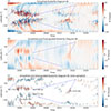 |
Fig. 10. Solar magnetic butterfly diagrams of the radial field (Br) from MDI and GONG data. (a) Smoothed butterfly diagram of Br, constructed from Carrington maps and combined datasets from SOHO/MDI and GONG. (b) Resolution-downgraded butterfly diagram, with latitudinal resolution reduced to match our observations of ι Hor (10° per pixel). (c) Field-weighted butterfly diagram. The location of each polarity is indicated, with error bars representing the standard deviation of field-strength-weighted latitudes. Linear fits with the corresponding speeds are indicated. |
Figure 10c is used to estimate the solar poleward flux transport speeds where five trends are identified and plotted. These trends try to replicate the two limiting cases we considered on ι Hor, with a fast lane following a given polarity surge to the pole right before its reversal (TK1, TK2, and TK5) and the slow lane starting from a given polarity region at mid-latitudes and following it to the polar region right after the reversal (TK3 and TK4). The tracks TK2 and TK5 roughly represent the accepted value for the meridional flow speed of the Sun, which varies around 10 m s−1 to 20 m s−1 (Hanasoge 2022). The speeds of the other three trends are much lower and they help gauge the values obtained from our observations of ι Hor, which are heavily limited by the gaps between epochs.
For the solar azimuthal field, we employ the butterfly diagram previously reconstructed by Cameron et al. (2018), which is shown in Fig. 11a. The diagram has a time resolution of one year and a latitudinal resolution of six degrees, which is downgraded by a factor of 2 to carry out our stellar-like analysis. We tracked the equatorial motions of each polarity in the field-weighted butterfly diagram as shown in Fig. 11b. Similar to ι Hor, we applied linear fits to the different polarity regions and obtain the equatorward drift speeds. The results are labeled beside the corresponding trends and they own an average speed of around 1.1 m s−1.
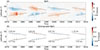 |
Fig. 11. Analysis of the solar equatorward drift based on the azimuthal magnetic field (Bϕ). (a) Reconstructed butterfly diagram for Bϕ taken from Cameron et al. (2018). (b) Downgraded butterfly diagram with half the original latitudinal resolution used for the analysis. The drift speeds of different polarity regions are determined via linear fits and are indicated by dashed lines. |
Based on the solar tests we see that the field-weighted latitudinal fitting procedure can roughly capture the accepted large-scale flow speeds on the Sun, with results falling within their nominal ranges. As mentioned earlier, for the poleward flux transport the solar analysis suggests that the slow tracks found in Sect. 3.3 most likely underestimate the flow speed in ι Hor. This is because the analogous solar tracks, TK3 and TK4, yield values close to one order of magnitude below the standard 10 − 20 m s−1 range. In this way, the fast speeds resulting from the analysis on ι Hor should be closer to the actual meridional flow on the star, which would surpass the solar values by factors between 4 − 7 approximately. Similarly, while the solar equatorward drift rate derived from our field-weighted butterfly diagram analysis appears slightly larger than global average obtained by Li et al. (2001), it falls right within the standard range measured at various latitudes and activity states (see, e.g., Hathaway et al. 2003). Note also that the linear fits applied here are a crude approximation of this solar observable, which can be better represented by a decaying exponential function as shown by Hathaway (2011). These results corroborate the robustness of our estimates on the equatorward migration drift obtained for ι Hor, placing it at about 17 − 22 times faster than its solar counterpart.
5. Summary
This paper presents our investigation of the magnetic cycle in the young solar analog ι Hor based on 18 ZDI maps acquired over nearly three years. We find clear changes in the large-scale surface magnetic field, including multiple polarity reversals and cyclic variations in both the poloidal and toroidal components. Dense ZDI sampling allowed us, for the first time, to obtain stellar magnetic butterfly diagrams that track the latitudinal migration of magnetic features and to derive initial estimates of large-scale flow properties on a star beyond the Sun (under the assumption of a similar flow phenomenology). These results provide useful benchmarks for models of dynamo processes in young solar-type stars.
Our analysis reveals a magnetic cycle intricately linked to the star’s activity. The ZDI reconstructions indicate that ι Hor undergoes a full magnetic cycle over roughly 100 rotations (∼2.1 yr), though latitudinal variations are evident – the polarity reversal timescales of some mid-latitude regions extend up to about 150 rotations in the radial component, while the azimuthal component oscillates on a slightly shorter timescale of around 90 rotations. In comparison, the chromospheric activity traced by the Ca II H&K S-index displays dual periodicities of approximately 70.7 rotations (∼1.49 yr) and 51.7 rotations (∼1.09 yr), suggesting a 2:1 correspondence for the shorter cycle and mirroring the relationship observed in the Sun. On the other hand, the coronal activity cycle traced by the X-ray emission indicates a periodicity of about 75.5 rotations (∼1.49 yr), which could be linked to the longer magnetic variability timescale identified in the butterfly diagrams of the radial magnetic field.
From a broader perspective, this work demonstrates how intensive spectropolarimetric monitoring can reveal the temporal evolution of stellar magnetism. By mapping variations in field strengths, geometry, and drift speeds, we can connect observed magnetic behavior to the underlying dynamo action. This approach can help advance the understanding of magnetic cycles in stars like ι Hor and lays the groundwork for future comparative studies with the solar cycle.
Data availability
The raw data associated with this project can be obtained from the ESO archive (http://archive.eso.org). The reduced spectropolarimetric sequences can be downloaded from the Polarbase repository (https://www.polarbase.ovgso.fr). The three sets of ZDI maps can be found in machine-readable format in the Zenodo repository with DOI: 10.5281/zenodo.17251923.
In practice, each epoch had an average of 11 quasi-consecutive nights (minimum of 8, maximum of 14) owing to bad weather conditions.
This value was chosen based on the approximate maximum latitudinal resolution expected for the ZDI reconstructions. With a rotational velocity vsin(i)≃6.5 km s−1 and a HARPSpol velocity spacing Δv = 0.8 km s−1 (R ≃ 110 000), the extracted LSD profiles of ι Hor encompass vsin(i)/Δv ≃ 8.125 resolution elements from the line center to the wing. Therefore, the 90° pole-to-equator angle is mapped by ZDI in latitudinal bins of 90° /8.125 ≃ 11° (Rozelot & Neiner 2016). This estimate neglects the variations due to the phase coverage of the individual ZDI maps (fairly consistent among all of our epochs) as well as the possible rotational smearing during the exposures (negligible in our observations).
Do not confuse with the meridional component of the magnetic field (not included in the butterfly diagram analysis).
This information was extracted from the individual ZDI maps.
There are not enough points in the negative polarity fast poleward model to perform a meaningful comparison.
Typically expressed as 1.6° yr−1, which we have converted to m s−1 assuming the fiducial value of the solar radius (R⊙ = 6.95 × 10⁸ m).
Acknowledgments
We would like to thank the anonymous referee for their constructive feedback, which helped improve the quality of this article. Based on observations collected at the European Organisation for Astronomical Research in the Southern Hemisphere under ESO programmes 096.D-0257, 097.D-0420, 098.D-0187, 099.D-0236, 0100.D-0535, and 0101.D-0465. Data were obtained from the ESO Science Archive Facility under request number jalvarad.212739. This work has made use of the VALD database, operated at Uppsala University, the Institute of Astronomy RAS in Moscow, and the University of Vienna. This research has made use of the SIMBAD database, operated at CDS, Strasbourg, France. J.D.A.G. would like to thank R. Cameron and M. Schüssler for providing the solar azimuthal magnetic field reconstruction. This research has made use of NASA’s Astrophysics Data System. J.D.A.G. and E.M.A.G. were partially supported by HST GO-15299 and GO-15512 grants. E.M.A.G and K.P. acknowledge support from the German Leibniz-Gemeinschaft under project number P67/2018 and support from the European Research Council (ERC) under grant agreement 101170037 (Evaporator). J.S.F. acknowledges support from the Agencia Estatal de Investigación of the Spanish Ministerio de Ciencia, Innovación y Universidades through grant PID2022-137241NB-C42.
References
- Alvarado-Gómez, J. D., Hussain, G. A. J., Grunhut, J., et al. 2015, A&A, 582, A38 [NASA ADS] [CrossRef] [EDP Sciences] [Google Scholar]
- Alvarado-Gómez, J. D., Hussain, G. A. J., Drake, J. J., et al. 2018, MNRAS, 473, 4326 [CrossRef] [Google Scholar]
- Amazo-Gómez, E. M., Alvarado-Gómez, J. D., Poppenhäger, K., et al. 2023, MNRAS, 524, 5725 [CrossRef] [Google Scholar]
- Aurière, M. 2003, in EAS Publications Series, eds. J. Arnaud, & N. Meunier, EAS Pub. Ser., 9, 105 [CrossRef] [EDP Sciences] [Google Scholar]
- Bagnulo, S., Landolfi, M., Landstreet, J. D., et al. 2009, PASP, 121, 993 [Google Scholar]
- Baliunas, S. L., Donahue, R. A., Soon, W. H., et al. 1995, ApJ, 438, 269 [Google Scholar]
- Baliunas, S. L., Henry, G. W., Donahue, R. A., Fekel, F. C., & Soon, W. H. 1997, ApJ, 474, L119 [NASA ADS] [CrossRef] [Google Scholar]
- Bellotti, S., Petit, P., Jeffers, S. V., et al. 2025, A&A, 693, A269 [NASA ADS] [CrossRef] [EDP Sciences] [Google Scholar]
- Blanco-Cuaresma, S., Soubiran, C., Heiter, U., & Jofré, P. 2014, A&A, 569, A111 [CrossRef] [EDP Sciences] [Google Scholar]
- Boro Saikia, S., Jeffers, S. V., Petit, P., et al. 2015, A&A, 573, A17 [NASA ADS] [CrossRef] [EDP Sciences] [Google Scholar]
- Boro Saikia, S., Jeffers, S. V., Morin, J., et al. 2016, A&A, 594, A29 [NASA ADS] [CrossRef] [EDP Sciences] [Google Scholar]
- Boro Saikia, S., Lueftinger, T., Jeffers, S. V., et al. 2018a, A&A, 620, L11 [NASA ADS] [CrossRef] [EDP Sciences] [Google Scholar]
- Boro Saikia, S., Marvin, C. J., Jeffers, S. V., et al. 2018b, A&A, 616, A108 [NASA ADS] [CrossRef] [EDP Sciences] [Google Scholar]
- Boro Saikia, S., Lüftinger, T., Folsom, C. P., et al. 2022, A&A, 658, A16 [NASA ADS] [CrossRef] [EDP Sciences] [Google Scholar]
- Brown, S. F., Donati, J.-F., Rees, D. E., & Semel, M. 1991, A&A, 250, 463 [NASA ADS] [Google Scholar]
- Brown, E. L., Marsden, S. C., Mengel, M. W., et al. 2021, MNRAS, 501, 3981 [NASA ADS] [CrossRef] [Google Scholar]
- Bruntt, H., Bedding, T. R., Quirion, P.-O., et al. 2010, MNRAS, 405, 1907 [NASA ADS] [Google Scholar]
- Cameron, R. H., Duvall, T. L., Schüssler, M., & Schunker, H. 2018, A&A, 609, A56 [NASA ADS] [CrossRef] [EDP Sciences] [Google Scholar]
- Carroll, T. A., Strassmeier, K. G., Rice, J. B., & Künstler, A. 2012, Astron. Astrophys., 548, A95 [Google Scholar]
- Chandrasekhar, S. 1961, Hydrodynamic and Hydromagnetic Stability (Oxford: Clarendon) [Google Scholar]
- Choudhuri, A. R. 2021, Sci. China Phys. Mech. Astron., 64 [Google Scholar]
- Coffaro, M., Stelzer, B., Orlando, S., et al. 2020, A&A, 636, A49 [EDP Sciences] [Google Scholar]
- Do Nascimento, J. D. Jr, Vidotto, A. A., Petit, P., et al. 2016, ApJ, 820, L15 [NASA ADS] [CrossRef] [Google Scholar]
- Domingo, V., Fleck, B., & Poland, A. I. 1995, Sol. Phys., 162, 1 [Google Scholar]
- Donati, J. F. 2003, in Solar Polarization, eds. J. Trujillo-Bueno, & J. Sanchez Almeida, ASP Conf. Ser., 307, 41 [Google Scholar]
- Donati, J. F. 2011, in Astrophysical Dynamics: From Stars to Galaxies, eds. N. H. Brummell, A. S. Brun, M. S. Miesch, & Y. Ponty, IAU Symp., 271, 23 [NASA ADS] [Google Scholar]
- Donati, J.-F., & Brown, S. F. 1997, A&A, 326, 1135 [NASA ADS] [Google Scholar]
- Donati, J.-F., & Landstreet, J. D. 2009, ARA&A, 47, 333 [NASA ADS] [CrossRef] [Google Scholar]
- Donati, J.-F., Semel, M., Carter, B. D., Rees, D. E., & Collier Cameron, A. 1997, MNRAS, 291, 658 [NASA ADS] [CrossRef] [Google Scholar]
- Donati, J.-F., Moutou, C., Farès, R., et al. 2008, MNRAS, 385, 1179 [CrossRef] [Google Scholar]
- Elsasser, W. M. 1946, Phys. Rev., 70, 202 [Google Scholar]
- Fares, R., Donati, J.-F., Moutou, C., et al. 2009, MNRAS, 398, 1383 [NASA ADS] [CrossRef] [Google Scholar]
- Fares, R., Donati, J.-F., Moutou, C., et al. 2010, MNRAS, 406, 409 [Google Scholar]
- Fares, R., Donati, J.-F., Moutou, C., et al. 2012, MNRAS, 423, 1006 [NASA ADS] [CrossRef] [Google Scholar]
- Fares, R., Moutou, C., Donati, J.-F., et al. 2013, MNRAS, 435, 1451 [NASA ADS] [CrossRef] [Google Scholar]
- Folsom, C. P., Petit, P., Bouvier, J., et al. 2016, MNRAS, 457, 580 [Google Scholar]
- Folsom, C. P., Bouvier, J., Petit, P., et al. 2018, MNRAS, 474, 4956 [NASA ADS] [CrossRef] [Google Scholar]
- Hackman, T., Lehtinen, J., Rosén, L., Kochukhov, O., & Käpylä, M. J. 2016, A&A, 587, A28 [NASA ADS] [CrossRef] [EDP Sciences] [Google Scholar]
- Hackman, T., Kochukhov, O., Viviani, M., et al. 2024, A&A, 682, A156 [NASA ADS] [CrossRef] [EDP Sciences] [Google Scholar]
- Hall, J. C., Lockwood, G. W., & Skiff, B. A. 2007, AJ, 133, 862 [Google Scholar]
- Hall, J. C., Henry, G. W., Lockwood, G. W., Skiff, B. A., & Saar, S. H. 2009, AJ, 138, 312 [NASA ADS] [CrossRef] [Google Scholar]
- Hanasoge, S. M. 2022, Liv. Rev. Sol. Phys., 19, 3 [Google Scholar]
- Harvey, J. W., Kennedy, J. R., & Leibacher, J. W. 1987, S&T, 74, 470 [Google Scholar]
- Harvey, J. W., Hill, F., Kennedy, J. R., Leibacher, J. W., & Livingston, W. C. 1988, Adv. Space Res., 8, 117 [CrossRef] [Google Scholar]
- Hathaway, D. H. 2011, Sol. Phys., 273, 221 [NASA ADS] [CrossRef] [Google Scholar]
- Hathaway, D. H. 2015, Liv. Rev. Sol. Phys., 12, 4 [Google Scholar]
- Hathaway, D. H., Nandy, D., Wilson, R. M., & Reichmann, E. J. 2003, ApJ, 589, 665 [NASA ADS] [CrossRef] [Google Scholar]
- Hatzes, A. P., Cochran, W. D., McArthur, B., et al. 2000, ApJ, 544, L145 [Google Scholar]
- Hébrard, É. M., Donati, J.-F., Delfosse, X., et al. 2016, MNRAS, 461, 1465 [CrossRef] [Google Scholar]
- Henry, G. W., Baliunas, S. L., Donahue, R. A., Fekel, F. C., & Soon, W. 2000, ApJ, 531, 415 [NASA ADS] [CrossRef] [Google Scholar]
- Hofmann, A., Strassmeier, K. G., & Woche, M. 2002, Astron. Nachr., 323, 510 [Google Scholar]
- Hotta, H., Bekki, Y., Gizon, L., Noraz, Q., & Rast, M. 2023, Space Sci. Rev., 219, 77 [NASA ADS] [CrossRef] [Google Scholar]
- Hussain, G. A. J., Donati, J.-F., Collier Cameron, A., & Barnes, J. R. 2000, MNRAS, 318, 961 [NASA ADS] [CrossRef] [Google Scholar]
- Hussain, G. A. J., van Ballegooijen, A. A., Jardine, M., & Collier Cameron, A. 2002, ApJ, 575, 1078 [Google Scholar]
- Hussain, G. A. J., Alvarado-Gómez, J. D., Grunhut, J., et al. 2016, A&A, 585, A77 [NASA ADS] [CrossRef] [EDP Sciences] [Google Scholar]
- Jeffers, S. V., & Donati, J. F. 2008, MNRAS, 390, 635 [CrossRef] [Google Scholar]
- Jeffers, S. V., Petit, P., Marsden, S. C., et al. 2014, A&A, 569, A79 [NASA ADS] [CrossRef] [EDP Sciences] [Google Scholar]
- Jeffers, S. V., Boro Saikia, S., Barnes, J. R., et al. 2017, MNRAS, 471, L96 [NASA ADS] [Google Scholar]
- Jeffers, S. V., Mengel, M., Moutou, C., et al. 2018, MNRAS, 479, 5266 [NASA ADS] [CrossRef] [Google Scholar]
- Jeffers, S. V., Cameron, R. H., Marsden, S. C., et al. 2022, A&A, 661, A152 [NASA ADS] [CrossRef] [EDP Sciences] [Google Scholar]
- Kochukhov, O. 2016, in Lecture Notes in Physics, Berlin Springer Verlag, eds. J. P. Rozelot, & C. Neiner (Springer), 914, 177 [Google Scholar]
- Kochukhov, O., & Piskunov, N. 2002, A&A, 388, 868 [CrossRef] [EDP Sciences] [Google Scholar]
- Kochukhov, O., Makaganiuk, V., & Piskunov, N. 2010, A&A, 524, A5 [NASA ADS] [CrossRef] [EDP Sciences] [Google Scholar]
- Kochukhov, O., Petit, P., Strassmeier, K. G., et al. 2017, Astron. Nachr., 338, 428 [Google Scholar]
- Kupka, F. G., Ryabchikova, T. A., Piskunov, N. E., Stempels, H. C., & Weiss, W. W. 2000, Balt. Astron., 9, 590 [Google Scholar]
- Lehmann, L. T., Hussain, G. A. J., Jardine, M. M., Mackay, D. H., & Vidotto, A. A. 2019, MNRAS, 483, 5246 [Google Scholar]
- Lehmann, L. T., Hussain, G. A. J., Vidotto, A. A., Jardine, M. M., & Mackay, D. H. 2021, MNRAS, 500, 1243 [Google Scholar]
- Lehtinen, J. J., Käpylä, M. J., Hackman, T., et al. 2022, A&A, 660, A141 [NASA ADS] [CrossRef] [EDP Sciences] [Google Scholar]
- Li, K. J., Yun, H. S., & Gu, X. M. 2001, AJ, 122, 2115 [Google Scholar]
- Liu, A. L., & Scherrer, P. H. 2022, ApJ, 927, L2 [Google Scholar]
- Marsden, S. C., Jardine, M. M., Ramírez Vélez, J. C., et al. 2011, MNRAS, 413, 1922 [Google Scholar]
- Marsden, S. C., Petit, P., Jeffers, S. V., et al. 2014, MNRAS, 444, 3517 [Google Scholar]
- Mayor, M., Pepe, F., Queloz, D., et al. 2003, The Messenger, 114, 20 [NASA ADS] [Google Scholar]
- Mengel, M. W., Fares, R., Marsden, S. C., et al. 2016, MNRAS, 459, 4325 [NASA ADS] [CrossRef] [Google Scholar]
- Mengel, M. W., Marsden, S. C., Carter, B. D., et al. 2017, MNRAS, 465, 2734 [CrossRef] [Google Scholar]
- Metcalfe, T. S., Basu, S., Henry, T. J., et al. 2010, ApJ, 723, L213 [NASA ADS] [CrossRef] [Google Scholar]
- Metcalfe, T. S., Buccino, A. P., Brown, B. P., et al. 2013, ApJ, 763, L26 [Google Scholar]
- Mittag, M., Robrade, J., Schmitt, J. H. M. M., et al. 2017, A&A, 600, A119 [NASA ADS] [CrossRef] [EDP Sciences] [Google Scholar]
- Mordvinov, A. V., Karak, B. B., Banerjee, D., et al. 2022, MNRAS, 510, 1331 [Google Scholar]
- Morgenthaler, A., Petit, P., Morin, J., et al. 2011, Astron. Nachr., 332, 866 [NASA ADS] [CrossRef] [Google Scholar]
- Morgenthaler, A., Petit, P., Saar, S., et al. 2012, A&A, 540, A138 [NASA ADS] [CrossRef] [EDP Sciences] [Google Scholar]
- Morin, J., Donati, J.-F., Petit, P., et al. 2008, MNRAS, 390, 567 [Google Scholar]
- Morin, J., Donati, J.-F., Petit, P., et al. 2010, MNRAS, 407, 2269 [Google Scholar]
- Petit, P., Dintrans, B., Solanki, S. K., et al. 2008, MNRAS, 388, 80 [NASA ADS] [CrossRef] [Google Scholar]
- Piskunov, N., & Kochukhov, O. 2002, A&A, 381, 736 [NASA ADS] [CrossRef] [EDP Sciences] [Google Scholar]
- Piskunov, N., Snik, F., Dolgopolov, A., et al. 2011, The Messenger, 143, 7 [NASA ADS] [Google Scholar]
- Poppenhaeger, K., Günther, H. M., & Schmitt, J. H. M. M. 2012, Astron. Nachr., 333, 26 [Google Scholar]
- Reiners, A. 2012, Liv. Rev. Sol. Phys., 9, 1 [Google Scholar]
- Robrade, J., Schmitt, J. H. M. M., & Favata, F. 2012, A&A, 543, A84 [NASA ADS] [CrossRef] [EDP Sciences] [Google Scholar]
- Rosén, L., Kochukhov, O., Hackman, T., & Lehtinen, J. 2016, A&A, 593, A35 [NASA ADS] [CrossRef] [EDP Sciences] [Google Scholar]
- Rosén, L., Kochukhov, O., & Wade, G. A. 2015, ApJ, 805, 169 [Google Scholar]
- Rozelot, J. P., & Neiner, C. 2016, Lecture Notes in Physics, Vol. 914, Cartography of the Sun and the Stars (Springer Nature Link) [Google Scholar]
- Ryabchikova, T., Piskunov, N., Kurucz, R. L., et al. 2015, Phys. Scr., 90 [Google Scholar]
- Sanz-Forcada, J., Stelzer, B., & Metcalfe, T. S. 2013, A&A, 553, L6 [NASA ADS] [CrossRef] [EDP Sciences] [Google Scholar]
- Sanz-Forcada, J., Stelzer, B., Coffaro, M., Raetz, S., & Alvarado-Gómez, J. D. 2019, A&A, 631, A45 [NASA ADS] [CrossRef] [EDP Sciences] [Google Scholar]
- Scherrer, P. H., Bogart, R. S., Bush, R. I., et al. 1995, Sol. Phys., 162, 129 [Google Scholar]
- Scherrer, P. H., Hoeksema, J. T., & Bush, R. I. 1991, Adv. Space Res., 11, 113 [Google Scholar]
- Schwarz, G. 1978, Ann. Stat., 6, 461 [Google Scholar]
- See, V., Jardine, M., Vidotto, A. A., et al. 2016, MNRAS, 462, 4442 [CrossRef] [Google Scholar]
- Semel, M. 1989, A&A, 225, 456 [NASA ADS] [Google Scholar]
- Skilling, J., & Bryan, R. K. 1984, MNRAS, 211, 111 [NASA ADS] [CrossRef] [Google Scholar]
- Strassmeier, K. G., Ilyin, I., Järvinen, A., et al. 2015, Astron. Nachr., 336, 324 [NASA ADS] [CrossRef] [Google Scholar]
- Švanda, M., Kosovichev, A. G., & Zhao, J. 2007, ApJ, 670, L69 [Google Scholar]
- Vauclair, S., Laymand, M., Bouchy, F., et al. 2008, A&A, 482, L5 [NASA ADS] [CrossRef] [EDP Sciences] [Google Scholar]
- Waite, I. A., Marsden, S. C., Carter, B. D., et al. 2015, MNRAS, 449, 8 [CrossRef] [Google Scholar]
- Waite, I. A., Marsden, S. C., Carter, B. D., et al. 2017, MNRAS, 465, 2076 [Google Scholar]
- Waldmeier, M. 1955, Ergebnisse und Probleme der Sonnenforschung [Google Scholar]
- Wargelin, B. J., Saar, S. H., Pojmański, G., Drake, J. J., & Kashyap, V. L. 2017, MNRAS, 464, 3281 [NASA ADS] [CrossRef] [Google Scholar]
- Willamo, T., Lehtinen, J. J., Hackman, T., et al. 2022, A&A, 659, A71 [NASA ADS] [CrossRef] [EDP Sciences] [Google Scholar]
Appendix A: A ZDI view of the evolution of the surface magnetic field
Epoch 1 (10.2015, campaign day 0, rotation 0 - fixed)
The large-scale field of this epoch is dominated by the radial component (BR), displaying values between −6.4 G to 5.1 G. The field is mostly concentrated in four regions with alternating polarity, covering from −30° up to 60° in latitude and varying extensions in longitude (∼ 30° up to 90°). The pole accessible to the observations (north) displays a weak radial field of negative polarity. A band of negative (east-west direction) azimuthal field (BA) covers the visible hemisphere of the star, with a maximum field strength of 5.8 G. The magnitude of the meridional field (BM) remains below 30% of the peak value associated with the radial component. The ZDI map reproduces the Stokes V LSD profiles down to an optimal χR2 = 1.10.
Epoch 2 (12.2015, campaign day 74.75, rotation 9.67)
This epoch shows some important evolution in the large-scale field with respect to the previous visit. The field strength increases reaching ±11 G and −12.0 G for BR and BA, respectively. The radial field displays a negative polarity region toward higher latitudes and the pole, with patches of positive polarity located at lower latitudes (±30°). The band of negative polarity in BA, observed in Epoch 1, appears stronger and more concentrated in latitude (0° to 30°), while two weaker bands of positive polarity (west-east direction) in BA can be seen in the remaining latitudes. The magnitude of BM reaches up to 70% of the maximum radial field, albeit much of this increase is associated with cross-talk. A χR2 = 1.55 is achieved by this ZDI reconstruction.
Epoch 3 (02.2016, campaign day 135.76, rotation 17.56)
The third map of the campaign reveals similarities with the reconstruction from Epoch 2. The maximum field strength remains close to the ±10 G level for BR and around −11 G in BA. A strong negative radial field is established at the north pole with several weaker mixed-polarity regions distributed close to the equator. The azimuthal field preserves the geometry from Epoch 2, although some weakening is visible in the high-latitude positive BA band. The maximum strength of BM decreases down to 40% of the peak radial field. The ZDI fit to the observations in this epoch reaches a χR2 = 1.75.
Epoch 4 (06.2016, campaign day 262.14, rotation 33.91)
Some weakening of the field in all components is observed in this epoch, with values down to ±7 G and ±4 G for BR and BA, respectively. While the geometry in the radial field largely resembles the previous visit, the strong mid-latitude ring of azimuthal field is not visible anymore whereas the high-latitude one strengthens. By examining the ZDI distributions obtained in Epochs 3 and 5, we believe that the weakening of the field could be partially introduced by the relatively poor phase coverage we had in this visit (no observations within 0 < Φ ≲ 0.4; see Fig. 4). This also generates significant cross-talk in BM, which reaches up to 65% of the maximum value for BR. The Stokes V LSD profiles are reproduced at the χR2 = 1.20 level in this epoch.
Epoch 5 (08.2016, campaign day 319.04, rotation 41.27)
The ZDI observations in this visit reveal an almost identical BR distribution as to Epoch 3, and to the geometry retrieved in Epoch 4 for the BA component. The magnitude of the radial field appears within −8 G < BR < 4 G, while for the azimuthal component ranges between ±3 G. The meridional component stays below 40% of the maximum radial magnetic field. The associated fit to the Stokes V LSD profiles yields a χR2 = 1.05 for this ZDI reconstruction.
Epoch 6 (09.2016, campaign day 345.01, rotation 44.63)
The geometry of the large-scale field does not show major evolution with respect to Epoch 5 (∼ 3.5 stellar rotations separate the two visits). The radial component strengthens to ±9 G while a high-latitude positive band of azimuthal field starts to form, with a field magnitude up to 4 G. The meridional component resembles closely the one observed in the previous visit. The large-scale field reconstruction reproduces the LSD profiles at the χR2 = 1.45 level. Notice that with 14 Stokes V profiles, this epoch has more exposures than any other visit of the campaign (Fig. B.1, top).
Epoch 7 (10.2016, campaign day 376.00, rotation 48.64)
As can be seen in the top-panel of Fig. 2, the distribution of the large-scale field is not too dissimilar from the previous epoch of observations. An important weakening of the radial component takes place (|BR|< 5 G) while the opposite occurs to the positive band of the azimuthal field, which is now fully formed at mid-latitudes ( G). The magnitude of the meridional component remains below 35% of the radial field. While the ZDI maps are similar to the first observed epoch of the campaign (separated by roughly one year), the reversal of the dominant polarity is BA is now evident. The magnetic field reconstruction reproduces the Stokes V LSD profiles down to a χR2 = 1.05.
Epoch 8 (12.2016, campaign day 436.86, rotation 56.51)
This epoch reveals the first polarity reversal in the radial component of the large-scale magnetic field. The polar and equatorial regions are dominated by the positive and negative polarity in BR, respectively, with field strength values ranging between ±5 G. The ring-like structure of positive polarity in BA persists and strengthens up to 7 G. The peak magnitude of BM reaches close to 50% of the radial field, indicating that some cross-talk is present in the reconstruction. A χR2 = 1.10 results from the model-to-data comparison for this visit.
Epoch 9 (02.2017, campaign day 483.78, rotation 62.58)
A global increase in the field strength is observed during this epoch, with little variation in terms of geometry with respect to the previous visit. The radial component reaches values close to ±10 G, while the band of positive field in BA peaks at 9 G. The retrieved values in BM remain within 50% of the radial field strength. The ZDI solution provides an LSD Stokes V fit at the χR2 = 1.20 level.
Epoch 10 (07.2017, campaign day 634.11, rotation 82.03)
As can be seen in Fig. 2, while the topology of the radial field persists compared to the last two epochs, a dramatic variation in the azimuthal field is observed in this visit. Not only the magnitude of the field decreases (|BA|< 3.5 G) but also the mid-latitude band of positive azimuthal field is almost completely replaced by relatively weak mix-polarity regions in BA. Still, an overall dominance of the negative polarity is seen, indicating in this way the onset of the second polarity reversal of this component over the course of the cycle. The radial component also shows some minor weakening, with |BR|≃ ± 7.0 G. The meridional component remains below 50% of the radial field strength. The final ZDI reconstruction provides a χR2 = 1.15 to the spectropolarimetric dataset.
Epoch 11 (08.2017, campaign day 661.11, rotation 85.53)
Being only 3.5 stellar rotations apart, the large-scale field in this epoch retains most of the properties observed in the previous visit. The field strengths in all components display similar values as in Epoch 10, with just a subtle increase in the surface coverage of the azimuthal field with negative polarity. An optimal χR2 = 0.90 is achieved from the associated ZDI fit of the observations in this visit.
Epoch 12 (09.2017, campaign day 713.10, rotation 92.25)
Minor evolution of the large-scale magnetic field is observed in this epoch. The radial and azimuthal components remain within BR ≃ ±5.8 G and −3.9 G ≤BA ≤ 0.8 G. While the geometry of BR stays largely unaltered, the distribution of BA displays a clear establishment of a negative polarity band at mid-latitudes (analogous to the one observed in Epochs 7 - 9). The meridional component stays under 45% of the radial field peak value. This ZDI reconstruction achieves a χR2 = 1.05 in comparison with the Stokes V LSD profiles.
Epoch 13 (11.2017, campaign day 768.82, rotation 99.46)
The distribution of the large-scale field continues to be dominated by a negative band of azimuthal field, which now covers an entire hemisphere. The radial component displays a similar configuration to the last visit, with a positive field located at the visible pole and latitudes close to the visibility limit. Still, it is possible to observe a small increase in the coverage of negative polarity regions at mid-latitudes. The magnitude of the field ranges between ±6 G for BR and −7.0 G ≤BA ≤ 1.4 G. The meridional component reaches up to 25% of the maximum radial field strength. The ZDI reconstruction reproduces the LSD Stokes V profiles down to a χR2 = 1.30.
Epoch 14 (12.2017, campaign day 809.83, rotation 104.76)
Close to 105 stellar rotations since the beginning of the campaign (∼2.22 yr), we detect the second polarity reversal in the radial component of the large-scale magnetic field. As such, the visible pole returns to a negative polarity in the radial field, while latitudes below the equator and close to the visibility limit display positive BR values. On the azimuthal component, it is possible to see the emergence of a positive polarity region close to the polar region, while the negative band of the azimuthal field, persistent in the last two epochs, strengthens and is pushed to lower latitudes. This global behavior is very similar to what was observed during Epochs 1-3, providing further evidence of the re-initiation of the magnetic cycle. The radial field takes values between −7.7 G and 8.7 G, whereas the azimuthal field varies between −13.0 G and 4.4 G. The meridional field shows a slight increase in magnitude, reaching up to 40% of the maximum azimuthal field. The ZDI fit of the spectropolarimetric data for this epoch achieves a χR2 = 1.30.
Epoch 15 (02.2018, campaign day 854.75, rotation 110.58)
After approximately 5 rotations, the large-scale magnetic field in Epoch 15 roughly matches the configuration observed in the previous visit. This includes the geometry of each of the field components, as well as their magnitudes (i.e., BR ≃ ±7.5 G, −16.4 G ≤BA ≤ 2.0 G). Only minimal variation is observed in the retrieved BM distribution. The ZDI map achieves a χR2 = 1.20 when compared with the observed Stokes V LSD profiles.
Epoch 16 (06.2018, campaign day 992.12, rotation 128.35)
The ZDI maps of this epoch reveal the almost complete disappearance of the mid-latitude band of the azimuthal field of negative polarity. As such, the magnitude of this component dramatically decreases, going down to −4.4 G ≤BA ≤ 1.9 G (∼ 12 G of variation in comparison with the previous visit). In contrast, the radial component shows similar features as in the previous visit, with a distribution tending to be more dipolar displaying a subtle increase in field strength (−8.9 G ≤BR ≤ 7.8 G). The meridional field stays below 40% of the maximum radial field. As indicated in Fig. B.3 (top panel), this reconstruction reproduces the observed LSD Stokes V profiles down to a χR2 = 0.95.
Epoch 17 (08.2018, campaign day 1028.09, rotation 133.0)
Relatively close in time to the previous epoch (< 5 stellar rotations), the large-scale magnetic field maps of this visit indicate a new reversal in the dominant polarity of the azimuthal component (from negative to positive). This reversal is the third one registered in BA during the campaign (with the first two detected during Epochs 3-4 and 9-10), indicating that the next magnetic cycle is well underway during these observations of our program. While the geometry of BR closely resembles the configuration observed in Epoch 16, a global reduction of the field strength is observed with −5.5 G ≤BR ≤ 3.5 G and −1.5 G ≤BA ≤ 3.3 G. The meridional field reaches only up to 35% of the maximum radial magnetic field. The LSD Stokes V profiles are reproduced down to an optimal χR2 = 0.95 by these ZDI reconstructions.
Epoch 18 (09.2018, campaign day 1063.07, rotation 137.5)
In this last observing epoch the ZDI maps do not show any major changes in the geometry or polarity dominance with respect of the behavior observed in the previous two visits. The radial field configuration roughly matches the one observed in Epoch 16 (∼ 10 rotations before), whereas the azimuthal one is more similar to the reconstruction in Epoch 17 (∼ 4.5 rotations before). Still, the dominant polarity in the azimuthal field appears more concentrated in a band-like structure, clearly resembling the behavior observed throughout the campaign. Some strengthening of the field is observed in all components with |BR|≤ ± 12 G and −3.8 G ≤BA ≤ 7.7 G. Some cross-talk is visible in the meridional component, which reaches up to 50% of the maximum radial field strength. These ZDI maps reproduce the observed LSD profiles down to a χR2 = 1.00.
Appendix B: Spectropolarimetric data and ZDI fits (Epochs 6-18)
Appendix C: Symmetric and antisymmetric ZDI reconstructions
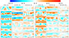 |
Fig. C.1. Maps of the large-scale magnetic field of ι Hor (in latitude-longitude equi-rectangular projection) favouring symmetry during the ZDI reconstruction for Epochs 1 to 12. Columns contain the radial (BR, left), azimuthal (BA, middle), and meridional (BM, right) field components, with the color scale indicating the magnitude (in gauss) and field polarity in each case. Each row corresponds to a different observing epoch, as indicated in the bottom right, with the observed phases denoted by black tick marks in longitude (upper x-axes). The campaign day and number of stellar rotations (measured from BJD = 2457300.78580 to the first night of observations of a given epoch) are listed on each map. The segmented line shows the visibility limit imposed by the inclination of the star (i = 60 deg). |
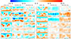 |
Fig. C.2. Same as Fig. C.1 but favouring for symmetry (Epochs 13 to 18; left) or antisymmetry (Epochs 1 to 6; right). |
All Tables
Properties of the large-scale magnetic field of ι Hor obtained from the ZDI reconstructions.
Best-fit parameters of the single-period sinusoidal models describing the evolution of the magnetic cycle in ι Hor.
All Figures
|
Fig. 1. Unconstrained ZDI reconstruction of the large-scale magnetic field maps of ι Hor in latitude-longitude equi-rectangular projection. Columns contain the radial (BR, left), azimuthal (BA, middle), and meridional (BM, right) field components, with the color scale indicating the magnitude (in gauss) and field polarity in each case. Each row corresponds to a different observing epoch, as indicated (Epochs 1 to 6), with the observed phases denoted by black tick marks in longitude (upper x-axes). The campaign day and number of stellar rotations (measured from BJD = 2457300.78580 to the first night of observations of a given epoch) are listed on each map. The segmented line shows the visibility limit imposed by the inclination of the star (i = 60 deg). |
| In the text | |
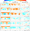 |
Fig. 2. Same as Fig. 1 but for Epochs 7 to 12. |
| In the text | |
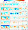 |
Fig. 3. Same as Fig. 1 but for Epochs 13 to 18. |
| In the text | |
|
Fig. 4. Recovered LSD profiles from the spectropolarimetric observations of ι Hor. Each row contains a different observing epoch (Epochs 1 to 5), with individual observing phases (Φ) shown in each subpanel. Left column: ZDI fits (red) to the circularly polarized data (Stokes V, black), with the optimal reduced χR2 achieved in each case. Right column: Corresponding diagnostic null (N) spectra. Both profiles have been enhanced (by a factor of 5.0 × 10³) and normalized to the continuum intensity (IC) for visualization purposes. The ZDI fits to the remaining epochs (6 to 18) are presented in Figs. B.1–B.3. |
| In the text | |
|
Fig. 5. Evolving global magnetic field properties for ι Hor plotted as a function of the chromospheric S-index and time. Top: Axisymmetry and log Btot2 for the total field. Middle and bottom: Axisymmetry and log B2 for the poloidal field and toroidal field components, respectively. The solid red line shows the best two-period model fit to Ca II H&K observations from Amazo-Gómez et al. (2023). Day “0” corresponds to BJD = 2457300.78580. The symbol sizes scale with log B2, and symbols for poloidal- and toroidal-dominated fields range from red to blue. The degree of non-axisymmetry is represented by symbol shapes, ranging from circular for a fully axisymmetric field and star-shaped symbols for non-axisymmetry. |
| In the text | |
|
Fig. 6. Similar to Fig. 5 but showing the evolution of the axisymmetric total energy, ⟨Baxi2⟩, and axisymmetric toroidal energy, ⟨Btor, axi2⟩, that most closely follow the evolution in the chromospheric activity (traced by the Ca II H&K S-index; dashed red line). |
| In the text | |
|
Fig. 7. Top and middle: Butterfly diagrams of the radial (top) and azimuthal (middle) large-scale magnetic field of ι Hor. These synoptic maps display the longitudinally averaged magnetic field strength (color bar, in gauss), extracted over 10° latitudinal strips on the individual ZDI epochs (Figs. 1 to 3). Bottom: Best two-period fit to the Ca II H&K S-index variations obtained by Amazo-Gómez et al. (2023). The shaded region encapsulates the 1σ period and amplitude uncertainties. Day “0” corresponds to BJD = 2457300.78580 (2015-10-05 06:51:33.12 UTC), and a secondary x-axis indicates the number of stellar rotations covered by the campaign (assuming Prot = 7.73 d). |
| In the text | |
|
Fig. 8. Temporal profiles of the longitudinally averaged radial (top) and azimuthal (bottom) large-scale magnetic field of ι Hor. Symbols and colors denote the range of latitudes of extraction, with error bars indicating the standard deviation of each component within the associated latitude strip as well as with longitude. Solid lines (with corresponding colors) show the resulting best-fit solution for a single-period model (three free parameters) at a given latitude bin (see text for details). |
| In the text | |
|
Fig. 9. Analysis of the large-scale flows on ι Hor based on the magnetic butterfly diagrams (Fig. 7) for the radial (top) and azimuthal (bottom) components. Individual points indicate the field-weighted mean latitude hosting each polarity at a given epoch, with error bars denoting its standard deviation within the averaged latitudinal bin. Filled colored circles and gray open diamonds indicate locations within the northern and southern hemispheres, respectively. The latitudinally averaged magnetic field strength, |
| In the text | |
|
Fig. 10. Solar magnetic butterfly diagrams of the radial field (Br) from MDI and GONG data. (a) Smoothed butterfly diagram of Br, constructed from Carrington maps and combined datasets from SOHO/MDI and GONG. (b) Resolution-downgraded butterfly diagram, with latitudinal resolution reduced to match our observations of ι Hor (10° per pixel). (c) Field-weighted butterfly diagram. The location of each polarity is indicated, with error bars representing the standard deviation of field-strength-weighted latitudes. Linear fits with the corresponding speeds are indicated. |
| In the text | |
|
Fig. 11. Analysis of the solar equatorward drift based on the azimuthal magnetic field (Bϕ). (a) Reconstructed butterfly diagram for Bϕ taken from Cameron et al. (2018). (b) Downgraded butterfly diagram with half the original latitudinal resolution used for the analysis. The drift speeds of different polarity regions are determined via linear fits and are indicated by dashed lines. |
| In the text | |
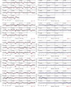 |
Fig. B.1. Same as Fig. 4 but for Epochs 6 to 10. |
| In the text | |
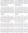 |
Fig. B.2. Same as Fig. 4 but for Epochs 11 to 15. |
| In the text | |
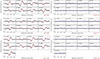 |
Fig. B.3. Same as Fig. 4. but for Epochs 16 to 18. |
| In the text | |
|
Fig. C.1. Maps of the large-scale magnetic field of ι Hor (in latitude-longitude equi-rectangular projection) favouring symmetry during the ZDI reconstruction for Epochs 1 to 12. Columns contain the radial (BR, left), azimuthal (BA, middle), and meridional (BM, right) field components, with the color scale indicating the magnitude (in gauss) and field polarity in each case. Each row corresponds to a different observing epoch, as indicated in the bottom right, with the observed phases denoted by black tick marks in longitude (upper x-axes). The campaign day and number of stellar rotations (measured from BJD = 2457300.78580 to the first night of observations of a given epoch) are listed on each map. The segmented line shows the visibility limit imposed by the inclination of the star (i = 60 deg). |
| In the text | |
|
Fig. C.2. Same as Fig. C.1 but favouring for symmetry (Epochs 13 to 18; left) or antisymmetry (Epochs 1 to 6; right). |
| In the text | |
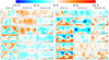 |
Fig. C.3. Same as Fig. C.1 but favouring antisymmetry for Epochs 7 to 18. |
| In the text | |
Current usage metrics show cumulative count of Article Views (full-text article views including HTML views, PDF and ePub downloads, according to the available data) and Abstracts Views on Vision4Press platform.
Data correspond to usage on the plateform after 2015. The current usage metrics is available 48-96 hours after online publication and is updated daily on week days.
Initial download of the metrics may take a while.