| Issue |
A&A
Volume 704, December 2025
|
|
|---|---|---|
| Article Number | A324 | |
| Number of page(s) | 21 | |
| Section | Numerical methods and codes | |
| DOI | https://doi.org/10.1051/0004-6361/202555629 | |
| Published online | 06 January 2026 | |
Identification of molecular line emission using convolutional neural networks
1
Laboratoire d’Astrophysique de Bordeaux, Univ. Bordeaux, CNRS, UMR 5804,
33615
Pessac,
France
2
LERMA, Observatoire de Paris, PSL Research University, CNRS, Sorbonne Univ., UMR 8262,
75014
Paris,
France
3
IRAM, 300 Rue de la Piscine,
38046
Saint Martin d’Hères,
France
★ Corresponding author: This email address is being protected from spambots. You need JavaScript enabled to view it.
Received:
22
May
2025
Accepted:
20
October
2025
Abstract
Context. Complex organic molecules (COMs) are found to be abundant in various astrophysical environments, particularly toward star-forming regions, where they are observed both toward protostellar envelopes as well as shocked regions. The emission spectrum, especially that of heavier COMs, might consist of up to hundreds of lines, where line blending hinders the analysis. However, identifying the molecular composition of the gas that leads to the observed millimeter spectra is the first step toward a quantitative analysis.
Aims. We have developed a new method based on supervised machine learning to recognize spectroscopic features of the rotational spectrum of molecules in the 3 mm atmospheric transmission band for a list of species including COMs, with the aim of obtaining a detection probability.
Methods. We used local thermodynamic equilibrium (LTE) modeling to build a large set of synthetic spectra of 20 molecular species, including COMs with a range of physical conditions typical for star-forming regions. We successfully designed and trained a convolutional neural network (CNN) that provides detection probabilities of individual species in the spectra.
Results. We demonstrate that the CNN model we developed has a robust performance to detect spectroscopic signatures from these species in synthetic spectra. We evaluated its ability to detect molecules according to the noise level, frequency coverage, and line-richness, as well as to test its performance for an incomplete frequency coverage with high detection probabilities for the tested parameter space, with no false predictions. Finally, we applied the CNN model to obtain predictions on observational data from the literature toward line-rich hot core-like sources, where the detection probabilities remain reasonable, with no false detections.
Conclusions. We demonstrate the use of CNNs in facilitating the analysis of complex millimeter spectra both on synthetic spectra, along with the first tests performed on observational data. Further analyses on its explainability, as well as calibration using a larger observational dataset, will help improve the performance of our method for future applications.
Key words: line: identification / methods: data analysis / stars: formation / ISM: molecules
© The Authors 2026
 Open Access article, published by EDP Sciences, under the terms of the Creative Commons Attribution License (https://creativecommons.org/licenses/by/4.0), which permits unrestricted use, distribution, and reproduction in any medium, provided the original work is properly cited.
This article is published in open access under the Subscribe to Open model. This email address is being protected from spambots. You need JavaScript enabled to view it. to support open access publication.
1 Introduction
Through the interplay of physical and chemical evolution of the interstellar medium, a variety of chemical species emerge, including complex organic molecules (COMs), such as sugars, alcohols, and aldehydes (see McGuire 2022, for a review). Their rotational (and, in certain conditions, vibrational) transitions in the (sub)millimeter range give access to these molecules in the gas phase. Based on decades of extensive observational efforts, the presence of chemical complexity across a broad range of astrophysical environments has been well established. Numerous species have been identified toward expanding shells of evolved stars (e.g., Kamiński et al. 2017), as well as nearby galaxies, where the emission of COMs has also been confirmed (e.g., Sewiło et al. 2018; Martín et al. 2021; Bouvier et al. 2025). Sensitive observations reveal COMs in various star-forming environments, such as Galactic dense cores (pre-stellar cores, hot cores, and hot corinos), shocks and extragalactic hot cores (for reviews, see e.g., Caselli & Ceccarelli 2012; Jørgensen et al. 2020; McGuire 2022; Ceccarelli et al. 2022; Shimonishi et al. 2023; Jimenez-Serra et al. 2025).
To identify emission from molecules other than the most abundant “simple” species, multiple transitions need to be detected. Accurately assigning molecular transitions to observed spectral lines may be challenging, especially in chemically rich environments. This is because heavier COMs with large partition functions exhibit a plethora of (rotational) transitions due to their molecular structure, implying a significant degeneracy in the potentially assigned transitions. Identifying the emission from such molecular species thus requires an iterative fitting process using models of radiative transfer calculations, typically assuming local thermodynamic equilibrium (LTE) conditions. Modeling spectral line transitions over a range of upper-level energies (Eup) enables estimates of the physical conditions, with a particular emphasis on precise column densities required to accurately infer molecular abundances (cf. Jørgensen et al. 2016; Mininni et al. 2020; Mercimek et al. 2022; Bouscasse et al. 2024; Belloche et al. 2025) enabling discussions of the chemical composition of astrophysical sources. Spectral surveys are particularly important in this aspect (e.g., Caux et al. 2011; Lefloch et al. 2018; Bouscasse et al. 2024; Belloche et al. 2025; Möller et al. 2025), since their broad frequency coverage allow for numerous transitions from the same species to be revealed.
Although LTE modeling tools are available (e.g., WEEDs, Maret et al. 2011; CASSIS, Vastel et al. 2015; XCLASS, Möller et al. 2017; MADCUBA, Martín et al. 2019; PySpecKit, Ginsburg & Mirocha 2011; molsim McGuire et al. 2024), to obtain a proper model of the spectra, molecules at the origin of the observed spectral lines need to be identified first. Subsequent iterative minimization methods in a step-by-step approach provide the best fit results (e.g., Möller et al. 2013; Qiu et al. 2025).
Systematic analyses of a large number of spectra are therefore hindered by several factors. For detailed examples, we refer to Bouscasse et al. (2022), Belloche et al. (2025) and Möller et al. (2025). These authors have also provided an in-depth discussion of spectral line analysis methods. In short, firstly, the initial line-fitting process is iterative and delicate if species need to be fitted individually. Secondly, a combination of limitations in the instrumental setup (e.g., the spectral resolution) and the source physical properties (e.g., the thermal and turbulent line widths) are essential in resolving individual spectral lines. Thirdly, identifying and fitting emission from each species must take into account the fact that the rotational spectra of COMs have several transitions that overlap in frequency even if individual spectral lines are resolved. This leads to line blending or line contamination, with the former corresponding to completely overlapping spectral lines that are not separable without proper modeling; whereas the latter allows us to identify the dominant line. Spectral confusion limit also needs to be considered, which occurs when emission from individual spectral lines cannot be distinguished due to a combination of the large number of spectral lines, as well as line overlap due to their turbulent and thermal line width, combined with an unresolved source structure. For example, spectral confusion was an issue for Sgr B2(N) (Belloche et al. 2013); however, resolving the source structure with ALMA reduced the intrinsic line widths, thereby mitigating spectral confusion (c.f. Belloche et al. 2022). The physical structure of the source may also lead to emission in multiple velocity components, while the temperature gradients and optical depth effects may result in non-Gaussian spectral line profiles. Other instrumental effects, such as spectral artifacts, contamination by strong emission lines from the other side-band, and discontinuous frequency coverage, add further complexity to the analysis.
Despite these challenges, new methods continue to emerge to facilitate the task of analyzing COM emission in the spectrum. Matched filtering and stacking (Loomis et al. 2018) help to increase the signal-to-noise ratio (S/N) to detect species (Loomis et al. 2021; McGuire 2022), while principal component analysis-based (PCA) filtering techniques may help to leverage complexity due to velocity components and line profiles (Yun & Lee 2023). An automated mixture analysis exploits the chemical relevance of a molecule to facilitate the identification of species in chemical mixtures (Fried & McGuire 2024).
This analytical approach can be complemented by data-driven approaches, particularly because machine learning methods have now been widely used for different areas in the field of astrochemistry, such as chemical modeling, reaction pathways, and computing binding energies (Villadsen et al. 2022; Heyl et al. 2023; Behrens et al. 2024; Wang et al. 2025). Furthermore, supervised and unsupervised machine learning techniques using vector representation of molecules have been developed to identify species with chemical similarity to those already detected in the ISM (Lee et al. 2021). Improving on this approach, Fried et al. (2023) and Scolati et al. (2023) included isotopologs and, by coupling it to LTE modeling, they predicted the molecular column densities. Successful applications have been demonstrated to infer the chemical inventories of IRAS16293 (Fried et al. 2023), Orion-KL (Scolati et al. 2023), and TMC-1 (Toru Shay et al. 2025). Using different machine learning methods on radiative transfer models, Mendoza et al. (2025) extracted information based on the line profiles of HCN and HNC molecules, while coupling chemical reaction calculations with neural networks. Another approach has been to use information field theory to infer which lines trace best specific conditions in the ISM to assist in observational campaigns (Einig et al. 2024). Grassi et al. (2025) coupled 1D collapse models to thermochemical modeling to connect model properties to specific tracers.
In other domains of astronomical spectroscopy, artificial neural networks (ANNs) have been efficiently used for X-ray (González-Martín et al. 2014; Dupourqué et al. 2024) and optical spectroscopic datasets (e.g., Bailer-Jones et al. 1997; Guiglion et al. 2024). Motivated by these advancements, we have aimed to develop a neural network-based approach to facilitate the analysis of complex spectroscopic (sub)millimetric data by significantly speeding up the line identification process in the millimeter spectral range providing a quasi-immediate prediction with respect to which COMs could be present in the spectrum. To our knowledge, this approach that has not yet been addressed in the literature.
We sought to design a multi-label classification method to detect and identify the spectral signature of other simple molecules as well as COMs within millimeter spectra with a focus on Galactic star-forming regions; specifically, hot core and hot corino-like environments. Although our main goal here is to tackle identification of abundant COMs, it has been necessary for the modeling approach to consider other simple organic and inorganic species, since their emission may blend with strong transitions of COMs, hindering their detection. Unlike the approach in other works, such as those by Lee et al. (2021) and Toru Shay et al. (2025), our methodology does not rely on underlying chemical models and, as such, the choice of the investigated species is arbitrary. Our objective is to demonstrate that a neural network can be trained and used to effectively discern the molecular composition of millimeter spectroscopic data focusing on the most abundant COM species exhibiting numerous transitions in their rotational spectrum.
The applicability of our method depends on the physical conditions and source types represented in the training set. We also include isotopologs and assume LTE conditions that is a commonly accepted analysis method for hot core-like sources (Rolffs et al. 2011; Giannetti et al. 2025, e.g., Jaber Al-Edhari et al. 2017; Duronea et al. 2019 for HC3N). While we demonstrate the applicability of our method using data from the IRAM 30m telescope, our approach is designed to be independent of the observing setup.
The paper is organized as follows. We describe the construction of the training set in Sect. 2 and present the convolutional neural network (CNN) architecture, along with its training and validation in Sect. 3. We demonstrate the capabilities and discuss the performance of the CNN model in Sect. 4. Applications to observational data are presented in Sect. 5.
2 Construction of the training set
Supervised machine learning methods rely on labeled training sets to learn the underlying data distribution. For millimeter spectra, however, we lack sufficiently large sets of labeled observational datasets that would be usable for training; hence, we need to rely on synthesized data where the physical parameters are well established and their labeling is unambiguous. However, the challenge is that such synthetic spectra represent several biases and, most importantly, they are incomplete in terms of molecular richness and might not adequately represent the source structure, while also lacking in potential observational artifacts.
We used LTE modeling to obtain synthetic spectra of a list of species that make up the focus of this study. This approach allowed us to explore a wide range of physical parameters and molecular compositions. The free parameters for our LTE models include the molecular column density (NX, where X represents different species), excitation temperature (Tex), kinematics of the gas (the rest velocity, vLSR, and line-width, ∆v), and the size of the emission for each species of the medium. These parameters led us to a system with a degree of freedom of n × 5 to model, where n is the number of molecules to consider. To systematically explore such a parameter space over a broad range of physical conditions is challenging. Therefore, we limited our approach to a handful of molecules that are widely abundant and have numerous rotational transitions in the millimeter spectral range. We then defined the physical parameter space to be representative of the conditions observed in star-forming regions.
Here, we focus on the rotational spectrum of molecules in a frequency range of 80–115 GHz that covers a substantial fraction of the 3 mm atmospheric transmission window. This frequency range is interesting since it has less severe line confusion compared to higher frequencies. We explicitly chose this frequency range to avoid the CO (J = 1–0) line at 115.271 GHz due to its ubiquitously complex line profile.
2.1 Molecular composition
Our aim here is to facilitate the identification of species where LTE modeling is necessary for their firm identification due to their large number of rotational transitions. Therefore, we focus on COMs that are among the most abundant species found toward star-forming regions and COMs that exhibit more than 100 rotational transitions in the considered frequency range above an Aij threshold and below an upper level energy of Eup/k < 500 K. These species are O-bearing COMs, such as CH3CHO, CH3COCH3, CH3OCH3, CH3OCHO, (CH2OH)2, and C2H5OH, and N-bearing COMs, such as C2H3CN, C2H5CN, C3H7CN, CH3NH2, and HC(O)NH2. All of these species are frequently detected toward chemically rich regions, such as hot molecular cores, hot corinos, and shocks (cf. Belloche et al. 2013; Jørgensen et al. 2020; Palau et al. 2017; Bouscasse et al. 2024; Vastel et al. 2024). The selected list of species corresponds to the most abundant COMs in these regions, yet it remains an arbitrary choice. For simplicity, we did not include S-bearing COMs, whose abundances are typically one to two orders of magnitude lower than those of COMs with analogous chemical structures. (e.g., Baek et al. 2022; Nazari et al. 2024).
For the sake of similarity with observational spectra, we add smaller COMs to this list, such as CH3OH and other abundant species, including CH3CCH, CH3CN, HC3N, H2CS, t-HCOOH, CH2NH, and NH2CN. They have lower number of rotational transitions (between 4 and 71) within our investigated limits of Eup/k and Aij. In addition, many of these species are also easily identified without LTE modeling. These molecules also provide a way to benchmark the capability of our method to identify emission from simpler species. We list the studied chemical species together with their number of rotational transitions in Table A.1.
2.2 LTE models
We computed LTE synthetic spectra for the 20 molecules discussed in Sect. 2.1 (and listed in Table A.1) for the investigated frequency range using the XCLASS software (Möller et al. 2017). The spectroscopic information was taken from the Cologne Database for Molecular Spectroscopy (CDMS; Müller et al. 2005; Endres et al. 2016) and Jet Propulsion Laboratory (JPL; Pickett et al. 1998) line catalogs as listed in Table A.1, for each species, respectively. Using LTE models is a commonly accepted approach to model emission from the majority of the here discussed COMs, firstly because toward the densest inner regions of hot cores and hot corinos LTE conditions are satisfied, but also because collisional rate coefficients are not systematically available for the heavier COMs in our sample1.
We fixed the source rest velocity (vLSR) to zero and used a spectral resolution of 1 MHz corresponding to ∼3 km s−1 giving a total of 35 000 channels for the frequency range between 85 and 115 GHz. Since we work directly with the frequency information, our model is applicable to any spectra with the proper vLSR correction applied (see Appendix E). We explored a column density range (NX) up to seven orders of magnitude, typically between 1012 and 1019 cm−2, corresponding to physical conditions commonly observed toward high-mass star-forming regions at scales up to a few thousands of au (for a review see Jørgensen et al. 2020). We sampled the column density range (NX) on a logarithmic scale using 40 points and (as discussed in Sect. 2.3) for certain species, we used a different parameter range. The column density for CH3OH was set to 1014–1020 cm−2 as this species has been observed as being abundant in star-forming regions; whereas for complex cyanides, we used a range of 1012–1018 cm−2 and for rarer molecules (ethylene glycol, propyl cyanide), we used 1012–1017 cm−2. We computed the models using five values of excitation temperature, corresponding to 30, 50, 100, 150, and 300 K, sampling both quiescent and heated protostellar environments. We sampled the line widths as 1, 3, 5, 10, and 12 km s−1. An important and specific parameter that often comes with poor constraints is the ratio between the size of the source and that of the telescope beam. This can only be constrained by mapping experiments that lead to spatially resolved measurements of the molecular emission. For distant (>1 kpc) high-mass star-forming regions, interferometric observations are typically required to measure the emission size of COMs. Treating the ratio between the source size and that of the telescope beam as a free parameter ensures that the models represent a broad range of observing configurations corresponding to both single-dish and interferometric measurements. For this purpose, we used a 3″ beam size and adopted a source size of 0.15, 0.3, 1.5, 3 and 15″, which corresponds to a range of source size over beam size between 0.05 and 5. This parameter range covers both interferometric observations with marginally or completely resolved source structures for both nearby or more distant regions (cf. Belloche et al. 2020; Feng et al. 2015; Bonfand et al. 2017; Giese et al. 2024, resp.), as well as unresolved emission typically corresponding to single-dish observations of more distant regions (e.g., Widicus Weaver & Friedel 2012; Widicus Weaver et al. 2017; Bouscasse et al. 2024).
For simplicity, we neglected any continuum emission other than the cosmic background radiation. Neglecting the contribution from moderately strong continuum radiation is not expected to hinder the line identification. Overall, we computed 5000 models per molecule. The LTE spectrum containing emission from multiple species was obtained by assuming that the spectra are linearly additive, which is a reasonable assumption for optically thin emission.
Transitions from molecular isotopologs may help the identification of their parent species by providing additional spectral lines, which can be a significant source of support for observations with a limited spectral bandwidth. Therefore, we also included in our LTE models the most abundant isotopologs of these species as listed in Table A.2, which were modeled together with their main isotopolog, implying that the physical parameters are the same. We took the standard local interstellar medium (ISM) values as fixed ratios. Our results are robust against variations in isotopic fractionation, as verified a posteriori under conditions typical of the Galactic Center (cf. Humire et al. 2020). We also took into account the lowest vibrationally excited states for CH3CN as well as those of CH3OH together with their isotopologs (cf. Table A.2). The ratios of the vibrationally excited states to the ground (v = 0) states were set to one.
2.3 Composite spectra
The training set was compiled from composite synthetic spectra generated by random linear combinations of LTE models from individual species. When adding the spectra of multiple species, we introduced a jitter by randomly shifting the spectrum up to two channels for each species in both red-shifted and blue-shifted directions to take into account that emission from different species may not originate from the same gas. To ensure diversity in the training set, the physical parameters of the spectra (excitation temperature, line width, source size over beam size) were independently varied for all species. Isotopologs that are modeled jointly with their main species are always accompanied by them. We also varied the number of species and column densities used for the composite spectrum (as discussed in detail in Sect. 2.4).
The inclusion of a thermal noise to the spectra is necessary to enable a meaningful application to observational data. Once the composite spectrum is created, we added a Gaussian noise where the standard deviation is sampled from a uniform distribution, giving an overall noise level that varies between 0.2 mK and 280 mK.
We also introduced additional features to the spectra with the aim of enhancing the robustness of the ANN model against unknown components and mimicking potential observational effects. First, we added fake emission lines that are randomly distributed in frequency to mitigate the effect of emission from species not included in our model. These fake lines account for between 5% and 10% of the total number of transitions within a given spectrum and they have a brightness temperature randomly drawn between 10 mK and 300 K, following a log-normal distribution. Second, we also added artificial negative Gaussian lines to the spectra corresponding to absorption features originating from either physical or instrumental effects. We randomly selected the number of absorption components for 50% of the training set, using between 1 and 10 Gaussian components with a mean line width of 2.75 MHz and amplitudes randomly sampled from a uniform distribution with values between 30% and 50% of the strongest line in the band.
We found that these adjustments to the training sample are crucial for our trained model to achieve good generalization. In particular, including a set of artificial lines in the spectra adds spectral noise (with positive and negative features) to the training set, which allows the ANN to better learn signal from species to be identified. Injecting these different forms of noise unrelated to molecular emission helps the network to be more robust against unknown transitions and, therefore, to be more adept at making predictions based on observational spectra (see Sect. 5).
A further step was to simplify the task of network training by masking a small frequency range around transitions from the most abundant simple molecules listed in Table A.3. This implies that we excluded these frequency ranges from the analysis. This was necessary because emission from several of these simple molecules is quasi omni-present in observational spectra, where COMs can be searched for. However, many of these species are expected to have optically thick emission in their low-J transitions and due to their high abundances, they are also sensitive probes of the gas kinematics leading to complex line profiles, where concrete examples include the 13CO, HCN, HNC, CS, SO, and N2H+ lines. Consequently, to enable a meaningful comparison to observational spectra, we masked ten channels centered on the rest frequency of their transitions. The number of transitions of COMs falling within these masks is listed in Table A.4, where we note that this eliminates typically <10% of their transitions; the only exception is CH3CN, where a more significant blending is noticed due to blended transitions from the weakest isotopolog, 15N.
Figure 1 shows an example resulting synthetic spectrum including emission from all investigated species with physical parameters corresponding to that of a typical hot core (see Table A.5) with lines having a width of 5 km s−1, a noise level of 50 mK assuming a source size that fills the 3″ beam. As discussed above, our main objective is to develop a method applicable to chemically rich Galactic star-forming regions, including hot cores. We show in Table A.5 how representative our parameter range is for such sources.
2.4 Constraining the training set
We created a training dataset of 4 × 10⁶ composite synthetic spectra by randomly sampling the 5000 LTE model spectra for each of the 20 investigated species and all other parameters as described in Sect. 2.2. We defined four subsets consisting of different molecular compositions: the first two follow a well-defined combination, the third is a random composition, and the fourth is a subset with just noise:
– The first subset of 106 spectra aims to be representative of molecular environments with having at least 10 from the 20 randomly selected molecules in each spectrum with astrochemically reasonable conditions resembling that of hot corinos and hot cores. Certain molecules are expected to be chemically related, such as sharing common molecular precursors or having the same functional groups (Garrod & Herbst 2006; Jørgensen et al. 2020), as well as observational results, lend support to correlated abundance ratios among specific COMs (e.g., Drozdovskaya et al. 2019; Coletta et al. 2020; Nazari et al. 2022; Bouscasse et al. 2024). Here, we take this into account by imposing column density ratios separately for O- and N-bearing molecular families, as
![Mathematical equation: ${{{N_{{\rm{col}}}}\left( {{\rm{O - bearing species}}} \right)} \over {{N_{{\rm{col}}}}\left( {{\rm{CH}}{ & _{\rm{3}}}{\rm{OH}}} \right)}}\, \in \,[{10^{ - 3}},\,{10^0}].$](/articles/aa/full_html/2025/12/aa55629-25/aa55629-25-eq1.png) (1)
(1)
For N-bearing species that may become abundant in the hot gas phase, such as C2H3CN, C2H5CN, HC3N, and HC(O)NH2, we have
![Mathematical equation: ${{{N_{{\rm{col}}}}\left( {{\rm{N - bearing species}}} \right)} \over {{N_{{\rm{col}}}}\left( {{\rm{C}}{{\rm{H}}_{\rm{3}}}\,{\rm{CN}}} \right)}}\, \in \,[{10^{ - 3}},\,{10^2}].$](/articles/aa/full_html/2025/12/aa55629-25/aa55629-25-eq2.png) (2)
(2)
For the rest of the species, such as NH2CN, CH3NH2, CH2NH, and C3H7CN, we have
![Mathematical equation: ${{{N_{{\rm{col}}}}\left( {{\rm{N - bearing species}}} \right)} \over {{N_{{\rm{col}}}}\left( {{\rm{C}}{{\rm{H}}_{\rm{3}}}\,{\rm{CN}}} \right)}}\, \in \,[{10^{ - 3}},\,{10^0}].$](/articles/aa/full_html/2025/12/aa55629-25/aa55629-25-eq3.png) (3)
(3)
The column density for H2CS and CH3CCH remains randomly drawn from the global column density range. Here, we use a broad range of abundance ratios that are globally consistent with observations (cf. Jørgensen et al. 2020; Belloche et al. 2025) and chemical model predictions (Garrod et al. 2022). We combined the spectra in such a way as to ensure that species with weak lines (a- and g-(CH2OH)2, C3H7CN, CH3NH2, and CH2NH) would be equally well represented in the final sample. This dataset is referred to as the “recipe” for the rest of the paper.
The second subset is also composed of 106 spectra, it is the same as the previous one but with a random gap within each synthetic spectrum which has a width of 200 to 800 MHz. The detection status is modified if transitions in these gaps impact the detectability of each species. One risk during training is that the network would only learn to recognize the few most obvious lines and neglect the others. Introducing these gaps forces the neural network to use less distinct attributes and to complete its information from other parts of the spectrum. Thus, this makes the model more efficient and robust to missing features.
We created a subset of 4 × 10⁵ spectra consisting of a random molecular composition and a noise distribution, as previously described. The role of this dataset is to expand the diversity of the produced spectra. This dataset is referred to as “unconstrained” throughout the paper, as no constraints were applied to the molecular content or physical parameters, which could lead to chemically unrealistic combinations of spectra.
The last subset is composed of 1.6 × 10⁶ spectra with only noise and artefacts, so that the ANN can also learn the properties of these components.
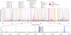 |
Fig. 1 Synthetic spectrum of a classical hot core computed from Table A.5 with a 5 km s−1 line width, a 50 mK Gaussian noise, and a zoom-in on 400 MHz. The LTE models are shown in color. The mask computed with the molecules from Table A.3 is in gray. The fake lines and absorption features are in blue and red, respectively. |
2.5 Labeling
The list of species used to obtain each combined synthetic spectrum provides a first initial labeling for the training set. However, thermal noise and the masking of transitions from simple, abundant species may reduce the detectability of the initially added molecules. Therefore, we revised the labeling to reflect the target values, which are determined by identifying the species that are detectable in each composite spectrum. We obtained the new labeling independently for each species by analyzing its individual spectrum prior to the linear combination, while still accounting for the thermal noise and masking frequencies corresponding to transitions from abundant omitted species. For a species to be considered detectable, we required that its spectrum contains at least two transitions with a peak intensity of ≥ 5σ, where σ is the dispersion of the Gaussian noise distribution added to the spectra. If the spectrum of a molecule fulfilled this detection criterion, it was flagged as detectable in the target vector of the corresponding composite spectrum.
We show the initial molecular composition of the “unconstrained” and “recipe” subsets of the synthetic spectra in Fig. B.1 as well as their revised labeling (constraining their target values). The obtained distribution for the molecular content on the whole training dataset is nearly uniform. The ANN sees between 106 and 2 × 10⁶ times each species during the training.
2.6 Validation and test datasets
We also created validation and test datasets each composed of 2 × 10⁴ synthetic spectra independently drawn from the training set. The molecular composition of these spectra correspond to 50% of our “recipe” and 50% of our “unconstrained” approach. We describe how we used the test dataset in Sect. 4 to evaluate the performance of the obtained ANN model.
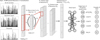 |
Fig. 2 CNN architecture scheme. Input data form an example of a composite spectrum according to the three normalizations, i.e., by the maximum (top), hyperbolic tangent (center), and polynomial (bottom). Filters are applied to the data to convolve the information and produce features maps. This operation is done for each of the convolutional layers. Dense layers then combine the extracted features and learn how to label the spectra depending on the provided target. The output layer is composed of one neuron per class giving a score between 0 and 1, independent of each other. |
3 Implementation of a CNN to learn spectral signatures
Our aim in this work is to build a tool that extracts the molecular composition from a millimeter spectrum based on their rotational transitions. For this purpose, we employed a classification model using a CNN architecture with supervised training (LeCun et al. 2015). In the following we discuss the implementation and training of this CNN.
3.1 Input and normalization for the CNN
To prepare the spectra for input into the neural network, we applied a normalization scheme widely used in machine learning applications, which allows the CNN to focus on pattern recognition by getting rid of the data scale and, thus, facilitates training convergence. The broad dynamic range of line intensities in the spectrum makes normalization by its maximum value less effective for CNNs learning their signatures. Therefore, we provided three different normalizations of the training set to the CNN, including two that highlight respectively weak and strong transitions. As illustrated in Fig. 2, the first transformation of the training set corresponds to a simple normalization, where each spectrum is normalized by its maximum value. The second transformation corresponds to a scaling where we compute the hyperbolic tangent of each spectrum multiplied by a factor α = 1.5, which is then normalized by its maximum value, increasing the contrast of weak lines. For the third transformation, we use a third degree polynomial of the normalized data to accentuate the features of strong lines. Therefore, a single spectrum is simultaneously injected to the network in these three forms of transformation.
Normalization was found to clearly influence the performance of the CNN model. The chosen methods were selected through testing to determine the most effective approach. In particular, we find that detection performances are systematically better when hyperbolic tangent normalization is combined with another one that preserves strong contrast in the maximum line intensity.
3.2 Neural network architecture
For this study, we designed a custom network architecture, which allows for finer control over the reduction rate of the spectral dimension compared to using a classical backbone. The optimum architecture was obtained empirically by starting with a very simple dense network and progressively increasing its depth and complexity. Systematic exploration of a gridded architectural space is very computationally expensive. Therefore, we used common substructures, setups, and possible adjunctions of layers as a baseline for our architecture and explored quite expansively the architectural space around that subspace.
The architecture mostly follows the classical scheme of forward classification models with a convolution part to extract non-localized patterns, and then a dense part that recombines the obtained features to predict the output classes. Figure 2 illustrates the structure of the 1D-CNN architecture. The convolutional layers were chosen to define the size of the receptive field at the end of the convolutional part to be of 8786 channels. It determines how the neural network filters and uses information from each single spectra (Araujo et al. 2019). Rotational transitions from asymmetric top molecules, such as most of the here investigated COMs, produce spectral features from the same molecule over the entire band, and hence we require the network to be able to process information from various parts of the spectra. We also include a few group normalization layers that improve the classification performance of our model (Wu & He 2018). These normalizations help to correlate information from all scales in the convolution axis (here, this is our 1D frequency axis) and also mitigate the risk of vanishing gradient issues. As with any layer normalization method, they also tend to speed up the training by reducing the number of iterations required to reach convergence.
Convolutional layers periodically apply a filter on their input according to a certain stride value. Thus, the network may give more importance to the signal coming from channels that fall on the central position of filters and/or channels that are involved in the activation of several filters when there is superposition. This effect is reinforced for an application such as ours where the position of the lines within the spectra is fixed, which can bias the network in its choice of important lines just by a geometric effect of the architecture. To avoid this, we add a jitter to the whole spectrum so that the peak of a line can be found on any element of the same filter. This amplitude is calculated as ![Mathematical equation: $ - \left[ {{{{k_1}} \over 2}} \right] \le x \le \left[ {{{{k_1}} \over 2}} \right]$](/articles/aa/full_html/2025/12/aa55629-25/aa55629-25-eq4.png) , where k1 is the size of the first filter, since it is the most sensitive to this effect. This also increments a translation invariance that could correspond to a potential error coming from the vLSR estimation in observational data. We find that this addition tends to stabilize our results over slight architectural changes that was not supposed to affect much the network expressivity.
, where k1 is the size of the first filter, since it is the most sensitive to this effect. This also increments a translation invariance that could correspond to a potential error coming from the vLSR estimation in observational data. We find that this addition tends to stabilize our results over slight architectural changes that was not supposed to affect much the network expressivity.
The convolutional part aims to extract coherent features in the spectra that are independent in their position in frequency space. These filters have a small number of parameters, but are applied to a large number of positions in the spectrum. Following a classical scheme, all the features identified by the convolutional part are then spatially recombined in the dense layers. As is common, most of the model parameters are located in the dense layers due to the flattening of feature maps into a single 1D vector. The second dense layer has a 40% dropout rate which supports this aspect as more neurons need to be declared to retrieve the same expressiveness as without dropout. This reinforces the disparity in the number of parameters between the convolutional and the dense part. The dropout is constantly activated during the training as a mean of regularization to avoid overfitting and to build a more robust model capable of generalization (Hinton et al. 2012).
During inference, dropout is usually deactivated with the weights of the associated layers scaled down to compensate for the extra number of activated neurons. This approach averages all the possible models that random dropout selection could create, predicting a single averaged output vector in a single inference step. An alternative approach is to keep the dropout activated at inference time and perform multiple inferences for each input vector. This allows us to build a distribution of model scores (see Sect. 4.5) from which we can predict a mean or median value and a dispersion that reflects the uncertainty of the prediction. This second approach is often referred to as Monte-Carlo dropout (Gal & Ghahramani 2015). Unless specified we always use the prediction obtained through model averaging.
The output layer is a dense layer composed of 20 neurons corresponding to the 20 molecules to be detected. We use a logistic (sigmoid) activation to obtain an independent model score for each of the neurons from this output layer. The stochasticity of the training will naturally push the network to predict a continuous value between 0 and 1 that will be proportional to its confidence in the presence of the molecule in a given input spectrum. Each class is represented by an output neuron independent from the activation of the other neurons of this final layer. To quantitatively interpret whether a given score value corresponds to a detection or non-detection of a molecule, we perform a “calibration” of the score values using the test dataset (see Sect. 4.4).
Our final architecture is presented in Table 1 and has a total of 1 957 989 parameters. It corresponds to the one presenting the best results while remaining computationally efficient. The network is implemented using the Convolutional Interactive Artificial Neural Networks by/for Astrophysicists (CIANNA) framework developed by Cornu (2025).
Detailed CNN structure for molecular detection as multi-label classification.
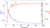 |
Fig. 3 Loss function computed on the validation dataset and AUC values as a function of training iterations with specified minimum loss and the corresponding AUC. |
3.3 CNN training
The initialization of weights is Glorot normal (Bengio & Glorot 2010). CIANNA optimizer uses a mini-batch stochastic gradient descent with momentum. We set the batch size to 32, and the learning rate, lr, follows an exponential decay to avoid oscillations around a minima or a too long convergence. It takes values from lr,start = 0.1 to lr,end = 10−3 with a decay d = 0.1. We set the momentum to 0.6 which accelerates convergence and reduces the fluctuation of loss values during learning through gradient descent (Qian 1999). We also add a small amount of weight decay λ which is set at 5 × 10⁻⁴.
We used a loss function that is defined as the mean squared error (MSE) estimated on the validation dataset to update the weights of the network during the training. The underfitting and overfitting were systematically checked during training with the help of the loss function computed over the validation dataset at each iteration (Fig. 3). Once the training was done, the model with the lowest loss was taken for inference. This step is also referred to as early stopping, which helps us avoid using an overfitted model.
As discussed in Sect. 2, we generated sufficient simulated data (i.e., a complete training set) to optimize its size for convergence, ensuring diversity so the network never sees the exact same spectrum twice. To handle this large sample size, we divided it into smaller portions, each corresponding to 1% of the whole training dataset processed during one iteration. We then performed 100 iterations for the training. With 4 × 10⁶ spectra in the training set and a computing precision of FP32C_FP32A, the training took 3.5 hours on a server equipped with one NVIDIA A100 GPU.
4 Results and analysis
4.1 Metrics
Here, we describe the metrics to evaluate the classification performance of the CNN model obtained during and after training. A first metric is the loss function that we use here on the test dataset. Figure 3 shows that the loss during the training decreases with the number of iterations. The MSE being an oversimplified metric, we also use other metrics such as the precision and recall that we calculate for each molecule as
 (4)
(4)
and
 (5)
(5)
However, these metrics require the predictions of our model to be expressed as a per-class binary classification. This can be obtained by considering a species detected if its model score is above a certain threshold.
By sampling the per-species recall and precision for different model score thresholds over the whole test dataset we build a precision recall curve (or ROC curve) for each species (using a 0.01 threshold sampling step), which are represented in Fig. 4. From this we also compute individual AUC (Area under the curve) values that are robust single value representations of the overall performances of the CNN model on each species. To estimate the overall performance we also compute a mean AUC over all the species. The AUCs are computed during and after training to obtain a scalar value which allowed us to optimize the network architecture (Bradley 1997). We represent the evolution of this mean AUC over training in Fig. 3 in comparison to the loss evolution demonstrating that the overall performance of the CNN model improves over iterations.
The training state with the lower MSE is taken for model inference as AUC values fluctuate and may reach high values during the training. The here presented CNN model is our best performing model with the minimum loss at iteration 99 and a mean AUC over the molecules of 0.904.
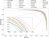 |
Fig. 4 ROC curves of the molecules for which the CNN learned to detect their spectral signature. The values are computed on a [0, 1] range from the x- and y-axis. |
4.2 Evaluation of the performance
The ROC curves show a simultaneously high recall and precision values for all species (Fig. 4), with a somewhat lower values for CH2NH. This allows us to conclude that the CNN model has a generally high performance for the detection of each species with few false detections and missed detections.
We train our CNN model three times with the exact same training setup but with different random starting weights to confirm the reproducibility of its results. In Fig. 5 we show the AUCs values for each species for the three independent trainings and find negligible variations. Their generally large (>0.89) values with a maximum dispersion of 0.04 allow us to conclude that the CNN model has a robustly high performance for the detection of each species. However, we find a lower mean AUC value (0.75) for CH2NH, compared to the other species. We investigate whether this is related to the number of spectra containing the respective molecule in the training sample (red crosses in Fig. 5), and find no clear correlation between the AUC values and the number of spectra with the given species. However, we find that one of the two bright transitions of CH2NH is blended with the mask from Sect. 2.3, meaning that this species is harder to detect unless the column density is high enough so the other transitions reach a sufficient S/N.
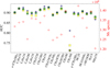 |
Fig. 5 AUC as a function of molecules for three trainings of the multi-labeling CNN. The squares, triangles, and stars are the AUC values. The red crosses correspond to the number of spectra where the molecules are detected. |
4.3 Impact of line density on the classifier performance
We investigated the performance of the CNN model as a function of line density using the spectra from the test dataset. For sources exhibiting a high molecular complexity, line density is a relatively straightforward metric for characterizing the spectra, which is applicable to both simulated and observational data. Here, we describe how we measured the line density of the spectra using the SciPyfind_peaks function that uses local maxima above a fixed 5σ threshold to extract the number of detected transitions. The line density was obtained by dividing the number of lines by our total frequency range of 35 GHz.
In Fig. 6, we compute the AUCs as a function of line density for the spectra. The CNN model shows a good performance for line-poor sources for molecules with only a few transitions, such as CH3CN, H2CS, and CH2NH with 11, 8 and 32 transitions, respectively (cf. Table A.1). We find that the mean AUC (of all species) increases with line density and from 2.97 lines per GHz, it is systematically above a value of 0.8 for 92.5% of the spectra. We recall that the higher the AUC value, the better the performance. Our results, therefore, suggest that the CNN model has a reliably high performance for a rather broad range of line densities. This behavior seems to indicate that the effect of line blending is marginal.
To set these line densities in context, we compared this range to that of the archetypal hot core, Sgr B2(N). Observed with the 30m telescope, Belloche et al. (2013) reported a line density of 102 lines per GHz for a frequency coverage of 79.990– 115.985 GHz, while at higher angular resolution with ALMA Bonfand et al. (2017) found a line density of 438 to 460 for its most prominent hot cores over a similar frequency range of 84.1–114.4 GHz. These frequency coverages are very similar to ours; however, their spectral resolution is higher by a factor of ∼2–3, hindering a direct comparison with these line density values. Resampling these spectra to a 1 MHz resolution would still preserve individual lines; however, line blending would likely decrease the number of lines when assuming the same noise threshold. Furthermore, Bonfand et al. (2017) uses a different approach to estimate line density, their values are therefore only approximately comparable to the line densities we measure here. The largest value for the line density that we measured in our test set is 162, while the mean and median line densities are 30 and 23, respectively. This suggests that the most extreme line rich sources are at the limit of our synthetic spectra, which is consistent with the fact that we consider here only the most abundant and, thus, a limited number of molecules of only 20 species. Although such a stable and reliable performance for a broad range of line densities was one of our objectives, we caution that spectra with higher complexity (i.e., more lines) may not be adequately treated by our current CNN model. A larger number of species must be considered in our model spectra to reach a line density similarly high to that of Sgr B2(N).
4.4 Calibration of the model score
In the previous sections, we discuss how we evaluated the global statistical performance of the CNN model based on the AUC, which is an averaged measure of a varying threshold for the model score. However, the results of the CNN model need to be interpreted for spectra where the target is not known. To do this, as described in Sect. 4.1, the score given by the final output layer can be converted to either a logical output (detection versus non detection) or a detection probability. We find that the latter is more informative on the ability of the model to identify the spectral signatures of molecules and, therefore, it is better suited for our applications.
To obtain a detection probability, we need to calibrate the model score using the test dataset (see Sect. 2.6). We apply our CNN model to the test dataset, that provides a list of detection scores between 0 and 1 for each spectrum, regardless of whether they contain the molecule or not. We then choose a score interval, for example 0.6 ± 0.01, for each species independently and select all the spectra with this model score. To convert this model score to a detection probability, we then evaluate the proportion of these selected spectra for which a detection of the species was expected, which can be expressed as
 (6)
(6)
By discretizing our [0,1] score interval we can compute a probability curve as a function of the predicted score for each species. We show an example obtained for the C2H5OH molecule in Fig. 7, where the detection probability scales roughly linearly with the model score. Based on our test dataset, we find a similar, roughly linear trend for all molecules. This linear scaling law is mostly the result of a relatively balanced training sample between the detectable and non-detectable cases. While this test confirms that we could use the detection score as a direct proxy for detection probability, this would not be the case for a different training set composition. In fact, the test set for calibrating the detection probability could be optimized if the range of physical conditions of the investigated source type is well defined. For the sake of consistency, we use the same calibration data set for all applications in this study. In the following, the value obtained by converting the model score through the calibration curve is called detection probability Pdet and is expressed in percentage.
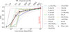 |
Fig. 6 Performance of the model as the AUC in function of line density. Color: mean AUC values for individual molecules. Black: mean global AUC value per bin. The number of spectra for AUC computation for each line density bin is specified. The line density of Sgr B2(N) observed with the 30m telescope (Belloche et al. 2013) is displayed as reference. |
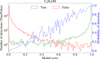 |
Fig. 7 Calibration curve for C2H5OH based on the number of true and false detections over the test dataset. |
4.5 Effect of the noise
In our simplified synthetic spectra, we expect thermal noise to be the dominant factor affecting the detectability of species, although line blending may also further reduce detectability. However, since we explore a broad range of column densities and source size over beam sizes, the detectability of molecules is not expected to scale linearly with the noise. Here we explore the impact of noise globally on the results of the CNN model by representing in Fig. 8 the AUC for each molecule as a function of noise in the test dataset. We find that the noise starts to have a impact above 20 mK resulting in a slight decrease in the AUCs, although the overall values remain still high above 0.85. As discussed in Sect. 4.2, CH2NH has systematically lower AUC values.
To investigate the impact of noise on detection probability, we use an example spectrum containing emission from all species (with the physical parameters listed in Table A.5, a 5 km s−1 line width and a source size equal to the beam size of 3″) without fake lines or absorption features, albeit with our initial mask from Sect. 2.3. We introduce three different noise levels of 100 mK, 500 mK, and 1 K, and extract the number of transitions with ≥ 5σ, as well as the S/N of the weakest such line from the LTE spectrum of each individual molecule. This is an important metric to evaluate the results of the CNN model, allowing us to compare our classical analysis approach with the CNN model prediction that leverages the entire rotational spectrum. Although the two highest noise levels are outside the range used for the training dataset, since we use normalized spectra as input, we do not expect this to have an impact on the predictions.
The detection probability provided by the CNN model is obtained through 100 realizations of MC-dropout on each of the three spectra. From these results, we take the median of the detection probabilities, and the median absolute deviation (MAD) as its uncertainty. In Table C.1, we present the manually extracted number of transitions above 5σ, along the corresponding minimum S/N of these lines, as well as the detection probability for each species provided by the CNN model. This serves as a sanity check to compare the model performance with expectations from the manual analysis.
We have a very high median detection probability for the lowest, 100 mK, noise level where highest probabilities are above 99% and with uncertainties <1% (with a 5% uncertainty for CH3COCH3). The exception is g-(CH2OH)2, where the detection probability is lower at 85% with uncertainties of 4–6%. These results stress the excellent performance of the CNN model on this highest S/N, highly idealized spectrum. Increasing the noise by a factor of 5, in this example spectrum, we end up losing detectable transitions from CH3COCH3 and g-(CH2OH)2. Although we would expect a detection probability of zero, the CNN model gives a detection probability of 25.4% with a large dispersion of about 10% for CH3COCH3. For g-(CH2OH)2, we obtain a low detection probability with a  value. Thus, the results for g-(CH2OH)2 are consistent with our expectations; however, for CH3COCH3 it is the significant median absolute deviation that suggests the non-detectability of the molecule. Considering the rest of the species, those impacted by the higher noise are a-(CH2OH)2, CH3OCHO, and CH2NH for which the CNN model gives a lower detection probability between 70 and 86%, with higher median absolute deviations reaching 4–12%. Finally, with a 1 K noise, many COM lines get below the 5σ detection threshold. Interestingly, the detection probabilities do not strictly correlate with the number of detectable transitions. For example, while for CH2NH, only three detectable transitions remain, we obtained a 72.7% detection probability with an uncertainty of a few percent. Similarly, C2H5OH has only 11 detectable transitions, but still presents a large probability with a median value of 81.6%. Whereas with six detectable lines for a-(CH2OH)2, we obtain only 24.8% detection probability and a large uncertainty. Visual inspection of the spectrum suggests that only three of these transitions are not blended or masked, and the CNN model uses two of them (see Sect. 4.7) to identify this molecule. These two lines are, however, weak and close to the detection limit of 5σ. Despite seven detectable transitions, the detection probability for CH3OCHO decreases to 38.5% with large errors. For the other species with a larger number of detectable transitions the detection probability still remains above 90% and with a negligible uncertainty.
Overall, we find that the detection probability is impacted by increasing the noise. As expected, the CNN model gives systematically the highest detection probabilities for species having ≥2 transitions at ≥ 5σ, that was imposed by our training set. We also find that the CNN model performance clearly does not solely depend on the number of detectable transitions. Nevertheless, our CNN model produces an excellent result for the example synthetic spectrum. In the following sections, we further evaluate the CNN model’s performance under various constraints on the input scenarios.
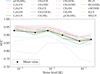 |
Fig. 8 Performance of the model as a function of noise. The AUC for each molecule is in color, while the average value over all species is in black. |
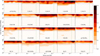 |
Fig. 9 Detection probability (average on 1000 realizations) as a function of the line density and the noise level. The blue horizontal line and the green vertical line correspond to the line density and noise limits of our training dataset. |
4.6 False positives
To test to which extent our model is susceptible to hallucination, that means predicting a false high detection probability, we apply it to fake synthetic spectra composed of various noise and random fake lines. We use a noise level and a fake line density on a grid of 10 × 10 values going from 2.5 × 10⁻⁵ K to 2.5 K, and 1 to 103 lines per GHz, both axis following a logarithmic scale. For each grid point, we create 1000 spectra with randomly distributed lines, line-width and intensity range, as in Sect. 2.3. We show in Fig. 9 the resulting mean detection probabilities for each grid point given by the CNN model.
The first result to note is that the detection probabilities are all below 10% for the parameter space constrained during the training. We also find that the noise level does not impact the detection probabilities, however, we do observe an increase in this value with increasing fake line density. Still, the detection probability remains below 50% even for the spectra with the maximum line density of 103. Although the fake lines are randomly distributed, we may expect that a significant number of channels with signal could mimic real emission of some species. Our results suggest that the CNN model takes into account other information than the position of lines, such as relative intensities. We can therefore conclude that false detections from our CNN model are unlikely to affect the reliability of the presented results, as long as the line density of the spectra remains in the range of our training sample.
12
4.7 Importance of features
To analyze the molecular content of millimeter spectra the modeled spectrum of each identified molecule was compared to the observed one. A simultaneous line-fitting was performed in an iterative process to firmly detect emission from a COM, especially from those with a large number of rotational transitions (such as (CH2OH)2, C3H7CN or CH3COCH3 from our list of targeted species). In contrast, it is more difficult to understand how the CNN model exactly computes its predictions since it is highly parametric. We aim here to explore the decision making process of our CNN model by hiding various fractions of spectral features and by doing an occlusion analysis.
We aim to evaluate how the number of transitions impacts the predicted probability for each species individually. We used the spectrum from Sect 2.3 (cf. Table A.5 with a 5 km s−1 line width and a 50 mK noise level) and randomly masked an increasing fraction of transitions from 20 to 90% by steps of 10% for each molecule separately. We performed 100 realizations with a different random set of masked lines each time and took the mean model score per molecule to obtain detection probabilities. This allowed us to mitigate the fact that different lines might have different levels of importance in the detection of a molecule due to brightness and line blending. The detection probability as a function of the fraction of hidden transitions is shown in Fig. 10 for each molecule. All species have a detection probability above 80% for less than 50% of their lines masked; however, the detection probabilities for all species show a decreasing trend with an increasing fraction of masked lines.
Above a 50% fraction of masked lines, the detection probability for CH3NH2 and C2H3CN drops. Interestingly, HC3N still has high detection probability, even when few or no transitions are present. Concerning the other species, the detection probability slightly decreases with the increasing fraction, but still remains above 50%. Overall, this result allows us to evaluate the resiliency of the CNN model to the degradation of the spectral features, but also the level of information redundancy that it learned from the spectra. Our results suggest that this is quite high, as we can mask a significant fraction of the lines while still being able to predict the presence of actual molecules with a high probability. In extreme cases, when masking too many transitions of the spectra becomes unrealistic and probably corresponds to unconstrained cases, which would explain some misinterpretations of the model.
However, randomly hiding a fraction of transitions does not allow us to estimate the importance of individual spectral features in the detection process. For this purpose, we perform an occlusion analysis that can help in testing the impact of each line on the model prediction. This analysis consists in masking a certain fraction of the signal, referred to as occlusion, and then evaluating the influence of this hidden signal on the CNN model’s classification. The method is illustrated schematically in Sect. D and Fig. D.1.
We perform this analysis using a sliding window of five channels, where we replace the real signal by the thermal noise of the spectra. We use a step size of three channels for the sliding window, and at each window position compute the difference between the original model score and the one obtained with occlusion. We thus obtain an "occlusion score" at the window position. This occlusion analysis is done for all species individually.
The highest the occlusion score, the more a feature is relevant for the detection. We show here the occlusion analysis for C2H5OH from the classical hot core synthetic spectrum (cf. Sect. 2.3). A positive occlusion score corresponds to a correlation made by the CNN model in favor of the molecule to be detected, while a negative score is linked to an anti-correlation. In Fig. 11, we compare the composite synthetic spectrum, the LTE model of C2H5OH and the occlusion score for a small frequency range around the maximum score. This demonstrates that peaks of the occlusion score coincide with transitions from the molecule of interest. Blended lines or lines from other species have a negative score, which reduces the probability of the molecule to be detected. Whereas a transition with a score equals to zero has no impact on the classification of the species.
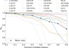 |
Fig. 10 Probability of detection (average on 100 realizations) for each molecule, depending on the fraction of intentionally hidden transitions. |
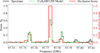 |
Fig. 11 First maximum of the occlusion analysis score for C2H5OH. |
4.8 Incomplete frequency coverage of observational setups
For our synthetic spectra, we used a complete spectral coverage between 80.0 and 115.0 GHz. Heterodyne receivers do not cover this frequency range instantaneously; for example, the EMIR receiver at the IRAM 30m telescope provides an instantaneous, noncontinuous bandwidth of about ∼15.5 GHz (Carter et al. 2012), which can be used to cover our investigated frequency range in two setups. Smaller frequency ranges can also be sufficient to firmly confirm emission from numerous COMs; therefore, we evaluated the performance of our CNN model on two possible setups from the EMIR receiver in the 3 mm band, noting that IRAM NOEMA also provides a very similar instantaneous frequency coverage. Our first setup covers a frequency range of 82–90 GHz and 98–106 GHz (setup 1), while the second setup covers a frequency range of 90–98 GHz, as well as 106– 114 GHz (setup 2). Since the CNN model was trained on spectra covering the full band of 80 to 115 GHz, using it on a limited spectral coverage of these setups does not come with adequate constraints, implying that the model score can no longer be calibrated or interpreted. To remedy this, it is necessary to readjust its task by implementing transfer learning through a complementary training for each setup of interest to recover a more efficient model. Using transfer learning instead of retraining the CNN from its initial state reduces training time and enables effective learning from limited data (e.g., Pan & Yang 2010; Domínguez Sánchez et al. 2018). Overall, this check demonstrates that our CNN model can be efficiently adapted to new observational setups with minimal computational cost.
This complementary training uses the CNN model parameters and redefines the output layer to avoid biases. For the rest, we used the same CNN architecture and the same hyperparameters. A special data set is produced for the desired setup with the same procedure as in Sect. 2 and the data target (i.e., labeling as discussed in Sect. 2.5) was adjusted based on the frequency coverage. Transfer learning was done independently for both setups and their combination, over ten iterations (10% of the number of examples from the original training). Combining the two setups nearly corresponds to the initially investigated full 80–115 GHz band.
To compare the performance of the CNN model for these setups, we used the diagnostic presented in Sect. 4.1. As in the previous sections (Sect. 4.7), we applied the CNN model to the classical hot core synthetic spectrum having a 50 mK noise level in the frequency ranges described above, and using MC-dropout. The number of 5σ transitions, the obtained median detection probability and the MAD for each molecule depending on the setup are presented in Table C.2. The results show a similarly high performance for both setups for the species that meet the detection criterion with typical detection probabilities above 84% for the majority. The HC3N molecule has only one detectable transition in setup 1 and consequently it has a detection probability of 50.0% with a maximum uncertainty of 8.6%. This means the molecule is potentially present; however, the CNN model does not have much confidence. On the other hand, HC3N has two transitions in setup 2 and the CNN model is able to robustly identify its spectral signature. The detection probability for CH3CCH is nearly zero in setup 2 as no transition lies within this frequency coverage. Similarly, the detection probability of NH2CN with one 5σ transition is low, 26.3%. When looking at the results of the combined setup, we find that the CNN model identifies well all molecules.
5 Application to observational data
5.1 Predictions using archival wide-band observational data
As shown in Sects. 4.3 and 4.5, our full 80–115 GHz band CNN model has a well-defined parameter space for the observed noise and line density. Sections 4.2 and 4.6 describe its performance on synthetic spectra, suggesting a high and reliable performance overall. Here, we aim to apply this model to observational data, that is a significant step forward in testing the applicability of our CNN model. In contrast to the synthetic spectra, observational data may contain emission from species not considered in our synthetic composite spectra and abundance ratios outside of that of our training set. Furthermore, gas kinematics above the 1 MHz resolution is neglected in our simulated data, which may hinder the detection performance of the CNN model.
We used observations obtained with the EMIR receiver at the IRAM 30m telescope toward chemically rich regions with hot-core characteristics from the literature that have a similar total frequency coverage as in our models and where a proper modeling of the spectra has already been performed. We investigated the archetypal hot cores Sgr B2(N) and B2(M) (Belloche et al. 2013), G34.26+0.15 (Csengeri et al. 2016), and the pre-hot core CygX-N63 (Fechtenbaum 2015). Since the CNN model is expected to be able to work on any continuous spectrum having the same frequency coverage and resolution as used for network training, it is expected to be applicable to interferometric data as well.
Basic data reduction steps had already been applied to the data, such as baseline subtraction and correcting the frequency axis for the source vLSR. The observational data have a spectral resolution better than 1 MHz and were, thus, first resampled to the same frequency axis and resolution as that of the training set. The preparation of input spectra to the CNN model is described in more detail in Appendix E. The noise was measured in both the original and the resampled spectra and we measured the line density according to the steps described in Sect. 4.3. We used the line density information to obtain an initial characterization of the spectra (see also Sect. 4.3) and to situate the observational data within the parameter space of the training set. As discussed in Belloche et al. (2013), the spectra of the Sgr B2 sources do not reach the confusion limit. Since the rest of the studied sources have lower line-widths and line densities, they are also above the confusion limit. The corresponding parameters of the used observational data are listed in Table 2.
We assigned a detection status for each source and species partly based on literature results and by re-analyzing the data as resampling could dilute the intensity of spectrally unresolved signal and increase the impact of line blending. For this, we visually inspected the resampled spectra and compare it with synthetic LTE models, however, we did this without performing a proper fitting because our results suggest little change in the overall detection of molecules toward these spectra. We list these results in Table 3 as either firm observational detections from the literature or as tentative detections, where a more precise modeling would be needed to confirm the detectability of these species.
Our CNN model was used to predict the molecular composition of the observational data. As described in Sect. 4.5, we applied the CNN model with 100 realizations of MC-dropout to obtain a median detection probability for each species listed in Table 3. We compared the detection probability of the CNN model for each molecule and we discuss these values in the context of the observational results in this paper.
5.1.1 Sgr B2(N)
We used the publicly available IRAM 30m observations from Belloche et al. (2013) to investigate the spectrum of Sgr B2(N). The CNN model predicts emission from C2H3CN, C2H5CN, C2H5OH, CH3CCH, CH3CN, CH3OCH3, CH3OCHO, CH3OH, HC3N, HC(O)NH2, H2CS, and NH2CN with a high detection probability of Pdet > 66%. On the other hand, it finds a very low detection probability for species that have weak, nevertheless observationally detectable signatures in the spectrum, such as a-(CH2OH)2, C3H7CN, CH3NH2, and CH2NH. This means that their transitions are difficult to identify. Considering our criteria of detectability, we would have expected the model to predict higher probabilities for these species. In addition, it gives a detection probability of 38.7% for CH3CHO, although with uncertainties of ∼9.2–12.9%, and 32.3% with similarly large uncertainties for CH3COCH3. From these examples CH3CHO is expected to be a relatively easily detectable species. g-(CH2OH)2 is predicted with a probability of 21.7%, with an error of ∼7–12% even though its spectral signature is observationally not confirmed. As shown in Sect 4.6, we find this kind of behavior when the CNN model is applied to a parameter range, or conditions it has not been trained for.
Observational data.
Detection probabilities obtained with MC dropout for millimeter data.
5.1.2 Sgr B2(M)
For Sgr B2(M), the results of the CNN model seem globally less convincing than for Sgr B2(N). The detection probability is generally lower for heavier COMs compared to Sgr B2(N), but high values (>80%) are found for more abundant species such as CH3CCH, CH3CN, CH3OH and HC3N. We find detection probabilities in the range of 35–50% for species, such as CH3CHO, CH3OCHO, HC(O)NH2, H2CS, and NH2CN. The error bars on these predictions are larger than ∼5.6–14.3, implying that the CNN model cannot properly predict the presence of these species toward this source. Nevertheless, it correctly predicts very low probabilities of <3% for non-detected species, such as t-HCOOH, a-(CH2OH)2 and g-(CH2OH)2.
This systematically low probability for molecules that should be identified suggests that the spectrum of this source is noticeably different from the training sample. When comparing the spectrum of Sgr B2(N) and Sgr B2(M), both have an important number of absorption lines due to foreground clouds (cf. Thiel et al. 2019). However, Sgr B2(M) exhibits significantly fewer spectral lines, making its overall characteristics less line-rich and the number of absorption lines compared to the emission lines more prominent compared to Sgr B2(N), and the training set.
5.1.3 G34.26+0.15
We also include in our analysis the archetypal hot core G34.26+0.15, where the spectrum is taken from Csengeri et al. (2016), and the molecular composition of this frequency range was already discussed in (Mookerjea et al. 2007, Widicus Weaver et al. 2017 for higher frequency observations). This source shows less complex kinematic features, and no significant absorption features from foreground clouds compared to the ones of Sgr B2 sources. We find that the predicted probability of our CNN model is high, ≳84% for C2H5CN, CH3CCH, CH3CN, CH3OCH3, CH3OCHO, CH3OH, HC3N, HC(O)NH2, and H2CS. Low detection probability of 2.7–21.6% is found for C2H5OH, CH3CHO, CH2NH and t-HCOOH with expected detections, while non-detections have low probability values.
5.1.4 CygX-N63
Here, we also investigate the spectrum of CygX-N63 that is a precursor of a hot core (Fechtenbaum 2015), a source that is less line-rich compared to the other ones with no absorption features. In this respect, this spectrum represents the simplest use case, where we expect reliable results. The CNN model detects high detection probabilities for CH3CCH, CH3CHO, CH3CN, CH3OH, H3CN, and H2CS. The COMs CH3OCH3 and HC(O)NH2 present probabilities slightly above 50%, whereas the others are less than 30% with CH3OCHO and t-HCOOH having a value around 20%. There are no false high probability detections, consistent with our previous results.
5.2 Applicability and limitation of the method
We successfully generalized our CNN model trained on synthesized data to observational data. Overall, we obtained large probabilities (> 50%) for most of the abundant species with expected detections and we did not find striking false positives for the investigated spectra, which is a very encouraging result. While the detection probabilities were typically higher (> 90%) for synthetic spectra on a well-constrained parameter space, we find lower detection probabilities corresponding to a range of 20–80% for observational data, which is likely due to the differences between real observations and our synthetic spectra. Low detection probabilities found for some COMs may be due to their signal being weaker than 5σ, and also due to significant line blending when resampling the spectra to 1 MHz resolution that is particularly limiting the application to sources such as Sgr B2(N). We notice a systematically lower performance of our CNN model for CH3NH2 and CH2NH which may come from blended lines as discussed in Sect. 4.2.
The CNN model presented in this paper was designed to detect molecules in rich millimeter spectra. The obtained results demonstrate that the CNN model is able to retrieve the spectroscopic fingerprint of species, although when applied to observational data, the most reliable results are obtained for the well known most abundant species. There is no evidence of any degraded performance caused by nonuniform noise over the band, nor by the line kinematics present in the observational data at >1 MHz resolution (e.g., as the strong absorption features for the Sgr B2 sources or high-velocity emission from outflows). We also could not identify any systematic trend in the performance that could be specific to a species.
The current version of the CNN model reaches its limits when applying to extreme sources such as for Sgr B2(N), a limitation that mostly comes from a large number of lines originating from species not included in our LTE modeling, and the spectral resolution that implies significant line blending. For the rest of the tested sources, such as G34.26+0.15 and CygX-N63, line blending is less of an issue, however, the spectral resolution used here is insufficient to resolve individual lines.
6 Conclusions
This study is aimed at validating the capacity of artificial neural networks to learn the spectroscopic signatures of various molecules using synthetic LTE model spectra. The main challenge has been to handle the large parameter space of the training set and optimize the architecture for the best performance. Our primary result is that the CNN model provides robust and reliable results on the synthetic data, demonstrating that it is able to learn signatures of rotational spectra specific to molecular species. The overall high performance indicates that our approach offers a meaningful way to identify the molecular content even in line-rich spectra.
We optimized the CNN model to be able to treat 20 species and a spectral resolution of 1 MHz for a frequency coverage of 80–115 GHz. Our analysis reveals that the CNN model performs well for a wide range of line density and noise. We also show that the CNN model takes into account not only the position of lines, but also the information from the entire spectrum to generate its predictions. A notable strength of our CNN model is its robustness against false positives.
We demonstrate that it is possible to adapt our CNN model to different frequency coverage ranges, corresponding to observational frequency ranges provided by the IRAM 30m and NOEMA telescopes through transfer learning. The application to observations has been validated with meaningful detection probabilities, confirming that CNN models are a promising approach to extracting information on the molecular composition of millimeter spectra. A better frequency sampling would increase the applicability of our model to even higher line density regimes and improve the treatment of line blending. Further improvements would require the development of more powerful CNN architectures and a training dataset that would include more molecular species. While the present work focuses on methodological development and validation, our approach opens a promising potential window to statistical applications on large datasets. Such approaches to CNN modeling will enable us to explore connections between molecular composition and source type, evolutionary stage, and galactic environment.
Acknowledgements
The authors thank the referee for their valuable comments, which significantly improved the manuscript. This study received financial support from the French government in the framework of the University of Bordeaux’s France 2030 program RRI Origins. N.K. acknowledges financial support from the AAP Doctorat Intelligence Artificielle (U. Bordeaux, ANR AI). T.Cs. received financial support from the French State in the framework of the IdEx Université de Bordeaux Investments for the future Program. This work was supported by the Programme National PCMI and PNPS of CNRS/INSU with INC/INP co-funded by CEA and CNES. Computer time for this study was provided by the computing facilities of the MCIA (Mésocentre de Calcul Intensif Aquitain).
References
- Araujo, A., Norris, W., & Sim, J. 2019, Distill, https://distill.pub/2019/computing-receptive-fields [Google Scholar]
- Baek, G., Lee, J.-E., Hirota, T., Kim, K.-T., & Kim, M. K. 2022, ApJ, 939, 84 [NASA ADS] [CrossRef] [Google Scholar]
- Bailer-Jones, C. A. L., Irwin, M., Gilmore, G., & von Hippel, T. 1997, MNRAS, 292, 157 [NASA ADS] [Google Scholar]
- Behrens, E., Mangum, J. G., Viti, S., et al. 2024, ApJ, 977, 38 [Google Scholar]
- Belloche, A., Müller, H. S. P., Menten, K. M., Schilke, P., & Comito, C. 2013, A&A, 559, A47 [NASA ADS] [CrossRef] [EDP Sciences] [Google Scholar]
- Belloche, A., Maury, A. J., Maret, S., et al. 2020, A&A, 635, A198 [NASA ADS] [CrossRef] [EDP Sciences] [Google Scholar]
- Belloche, A., Garrod, R. T., Zingsheim, O., Müller, H. S. P., & Menten, K. M. 2022, A&A, 662, A110 [NASA ADS] [CrossRef] [EDP Sciences] [Google Scholar]
- Belloche, A., Garrod, R. T., Müller, H. S. P., et al. 2025, A&A, 698, A143 [NASA ADS] [CrossRef] [EDP Sciences] [Google Scholar]
- Bengio, Y. & Glorot, X. 2010, International Conference on Artificial Intelligence and Statistics, 249 [Google Scholar]
- Bonfand, M., Belloche, A., Menten, K. M., Garrod, R. T., & Müller, H. S. P. 2017, A&A, 604, A60 [NASA ADS] [CrossRef] [EDP Sciences] [Google Scholar]
- Bouscasse, L., Csengeri, T., Belloche, A., et al. 2022, A&A, 662, A32 [NASA ADS] [CrossRef] [EDP Sciences] [Google Scholar]
- Bouscasse, L., Csengeri, T., Wyrowski, F., Menten, K. M., & Bontemps, S. 2024, A&A, 686, A252 [NASA ADS] [CrossRef] [EDP Sciences] [Google Scholar]
- Bouvier, M., Viti, S., Mangum, J. G., et al. 2025, A&A, 698, A261 [NASA ADS] [CrossRef] [EDP Sciences] [Google Scholar]
- Bradley, A. P. 1997, Pattern Recognit., 30, 1145 [Google Scholar]
- Carter, M., Lazareff, B., Maier, D., et al. 2012, A&A, 538, A89 [NASA ADS] [CrossRef] [EDP Sciences] [Google Scholar]
- CASA Team (Bean, B., et al.) 2022, PASP, 134, 114501 [NASA ADS] [CrossRef] [Google Scholar]
- Caselli, P., & Ceccarelli, C. 2012, A&A Rev., 20, 56 [NASA ADS] [CrossRef] [Google Scholar]
- Caux, E., Kahane, C., Castets, A., et al. 2011, A&A, 532, A23 [NASA ADS] [CrossRef] [EDP Sciences] [Google Scholar]
- Ceccarelli, C., Codella, C., Balucani, N., et al. 2022, arXiv e-prints, [arXiv:2206.13270] [Google Scholar]
- Chin, Y. N., Henkel, C., Whiteoak, J. B., Langer, N., & Churchwell, E. B. 1996, A&A, 305, 960 [NASA ADS] [Google Scholar]
- Coletta, A., Fontani, F., Rivilla, V. M., et al. 2020, A&A, 641, A54 [NASA ADS] [CrossRef] [EDP Sciences] [Google Scholar]
- Cornu, D. 2025, CIANNA: Convolutional Interactive Artificial Neural Networks by/for Astrophysicists, Astrophysics Source Code Library [record ascl:2501.005] [Google Scholar]
- Csengeri, T., Leurini, S., Wyrowski, F., et al. 2016, A&A, 586, A149 [NASA ADS] [CrossRef] [EDP Sciences] [Google Scholar]
- Domínguez Sánchez, H., Huertas-Company, M., Bernardi, M., et al. 2018, MNRAS, 484, 93 [Google Scholar]
- Drozdovskaya, M. N., van Dishoeck, E. F., Rubin, M., Jørgensen, J. K., & Altwegg, K. 2019, MNRAS, 490, 50 [Google Scholar]
- Dupourqué, S., Clerc, N., Pointecouteau, E., et al. 2024, A&A, 687, A58 [NASA ADS] [CrossRef] [EDP Sciences] [Google Scholar]
- Duronea, N. U., Bronfman, L., Mendoza, E., et al. 2019, MNRAS, 489, 1519 [CrossRef] [Google Scholar]
- Einig, L., Palud, P., Roueff, A., et al. 2024, A&A, 691, A109 [NASA ADS] [CrossRef] [EDP Sciences] [Google Scholar]
- Endres, C. P., Schlemmer, S., Schilke, P., Stutzki, J., & Müller, H. S. P. 2016, J. Mol. Spectrosc., 327, 95 [NASA ADS] [CrossRef] [Google Scholar]
- Fechtenbaum, S. 2015, PhD thesis, Université de Bordeaux, thèse de doctorat dirigée par Bontemps, Sylvain Astrophysique, plasmas, nucléaire Bordeaux [Google Scholar]
- Fechtenbaum, S., Bontemps, S., Schneider, N., et al. 2015, A&A, 574, L4 [NASA ADS] [CrossRef] [EDP Sciences] [Google Scholar]
- Feng, S., Beuther, H., Henning, T., et al. 2015, A&A, 581, A71 [NASA ADS] [CrossRef] [EDP Sciences] [Google Scholar]
- Fried, Z. T., & McGuire, B. A. 2024, J. Phys. Chem. A, 128, 8254 [Google Scholar]
- Fried, Z. T. P., Lee, K. L. K., Byrne, A. N., & McGuire, B. A. 2023, Digit. Discov., 2, 952 [Google Scholar]
- Gal, Y., & Ghahramani, Z. 2015, arXiv e-prints [arXiv:1506.02142] [Google Scholar]
- Garrod, R. T., & Herbst, E. 2006, A&A, 457, 927 [NASA ADS] [CrossRef] [EDP Sciences] [Google Scholar]
- Garrod, R. T., Jin, M., Matis, K. A., et al. 2022, ApJS, 259, 1 [NASA ADS] [CrossRef] [Google Scholar]
- Giannetti, A., Leurini, S., Schisano, E., et al. 2025, A&A, 698, A90 [NASA ADS] [CrossRef] [EDP Sciences] [Google Scholar]
- Giese, M. M., Thompson, W. E., Lis, D. C., & Widicus Weaver, S. L. 2024, ApJ, 960, 6 [Google Scholar]
- Ginsburg, A., & Mirocha, J. 2011, PySpecKit: Python Spectroscopic Toolkit, Astrophysics Source Code Library [record ascl:1109.001] [Google Scholar]
- González-Martín, O., Díaz-González, D., Acosta-Pulido, J. A., et al. 2014, A&A, 567, A92 [NASA ADS] [CrossRef] [EDP Sciences] [Google Scholar]
- Grassi, T., Padovani, M., Galli, D., et al. 2025, A&A, 702, A71 [NASA ADS] [CrossRef] [EDP Sciences] [Google Scholar]
- Guiglion, G., Nepal, S., Chiappini, C., et al. 2024, A&A, 682, A9 [NASA ADS] [CrossRef] [EDP Sciences] [Google Scholar]
- Heyl, J., Butterworth, J., & Viti, S. 2023, MNRAS, 526, 404 [NASA ADS] [CrossRef] [Google Scholar]
- Hinton, G. E., Srivastava, N., Krizhevsky, A., Sutskever, I., & Salakhutdinov, R. R. 2012, arXiv e-prints [arXiv:1207.0580] [Google Scholar]
- Humire, P. K., Thiel, V., Henkel, C., et al. 2020, A&A, 642, A222 [NASA ADS] [CrossRef] [EDP Sciences] [Google Scholar]
- Jaber Al-Edhari, A., Ceccarelli, C., Kahane, C., et al. 2017, A&A, 597, A40 [NASA ADS] [CrossRef] [EDP Sciences] [Google Scholar]
- Jimenez-Serra, I., Codella, C., & Belloche, A. 2025, arXiv e-prints [arXiv:2503.17104] [Google Scholar]
- Jørgensen, J. K., van der Wiel, M. H. D., Coutens, A., et al. 2016, A&A, 595, A117 [Google Scholar]
- Jørgensen, J. K., Belloche, A., & Garrod, R. T. 2020, ARA&A, 58, 727 [Google Scholar]
- Kamiński, T., Menten, K. M., Tylenda, R., et al. 2017, A&A, 607, A78 [NASA ADS] [CrossRef] [EDP Sciences] [Google Scholar]
- LeCun, Y., Bengio, Y., & Hinton, G. 2015, Nature, 521, 436 [Google Scholar]
- Lee, K. L. K., Patterson, J., Burkhardt, A. M., et al. 2021, ApJ, 917, L6 [NASA ADS] [CrossRef] [Google Scholar]
- Lefloch, B., Bachiller, R., Ceccarelli, C., et al. 2018, MNRAS, 477, 4792 [Google Scholar]
- Loomis, R. A., Öberg, K. I., Andrews, S. M., et al. 2018, AJ, 155, 182 [Google Scholar]
- Loomis, R. A., Burkhardt, A. M., Shingledecker, C. N., et al. 2021, Nat. Astron., 5, 188 [NASA ADS] [CrossRef] [Google Scholar]
- Maret, S., Hily-Blant, P., Pety, J., Bardeau, S., & Reynier, E. 2011, A&A, 526, A47 [NASA ADS] [CrossRef] [EDP Sciences] [Google Scholar]
- Martín, S., Martín-Pintado, J., Blanco-Sánchez, C., et al. 2019, A&A, 631, A159 [Google Scholar]
- Martín, S., Mangum, J. G., Harada, N., et al. 2021, A&A, 656, A46 [NASA ADS] [CrossRef] [EDP Sciences] [Google Scholar]
- McGuire, B. A. 2022, ApJS, 259, 30 [NASA ADS] [CrossRef] [Google Scholar]
- McGuire, B. A., Xue, C., Lee, K. L. K., El-Abd, S., & Loomis, R. A. 2024, molsim [Google Scholar]
- Mendoza, E., Dall’Olio, P., Coelho, L. S., et al. 2025, A&A, 698, A286 [NASA ADS] [CrossRef] [EDP Sciences] [Google Scholar]
- Mercimek, S., Codella, C., Podio, L., et al. 2022, A&A, 659, A67 [NASA ADS] [CrossRef] [EDP Sciences] [Google Scholar]
- Milam, S. N., Savage, C., Brewster, M. A., Ziurys, L. M., & Wyckoff, S. 2005, ApJ, 634, 1126 [Google Scholar]
- Mininni, C., Beltrán, M. T., Rivilla, V. M., et al. 2020, A&A, 644, A84 [NASA ADS] [CrossRef] [EDP Sciences] [Google Scholar]
- Möller, T., Bernst, I., Panoglou, D., et al. 2013, A&A, 549, A21 [NASA ADS] [CrossRef] [EDP Sciences] [Google Scholar]
- Möller, T., Schilke, P., Sánchez-Monge, Á., & Schmiedeke, A. 2025, A&A, 693, A160 [NASA ADS] [CrossRef] [EDP Sciences] [Google Scholar]
- Mookerjea, B., Casper, E., Mundy, L. G., & Looney, L. W. 2007, ApJ, 659, 447 [Google Scholar]
- Müller, H. S. P., Schlöder, F., Stutzki, J., & Winnewisser, G. 2005, J. Mol. Struct., 742, 215 [Google Scholar]
- Möller, T., Endres, C., & Schilke, P. 2017, A&A, 598, A7 [NASA ADS] [CrossRef] [EDP Sciences] [Google Scholar]
- Nazari, P., Meijerhof, J. D., van Gelder, M. L., et al. 2022, A&A, 668, A109 [NASA ADS] [CrossRef] [EDP Sciences] [Google Scholar]
- Nazari, P., Cheung, J. S. Y., Asensio, J. F., et al. 2024, A&A, 686, A59 [NASA ADS] [CrossRef] [EDP Sciences] [Google Scholar]
- Palau, A., Walsh, C., Sánchez-Monge, Á., et al. 2017, MNRAS, 467, 2723 [NASA ADS] [Google Scholar]
- Pan, S. J., & Yang, Q. 2010, IEEE Trans. Knowl. Data Eng., 22, 1345 [Google Scholar]
- Penzias, A. A. 1981, ApJ, 249, 518 [Google Scholar]
- Pickett, H. M., Poynter, R. L., Cohen, E. A., et al. 1998, J. Quant. Spec. Radiat. Transf., 60, 883 [Google Scholar]
- Qian, N. 1999, Neural Netw., 12, 145 [Google Scholar]
- Qiu, Y., Zhang, T., Möller, T., et al. 2025, ApJS, 277, 21 [Google Scholar]
- Rolffs, R., Schilke, P., Zhang, Q., & Zapata, L. 2011, A&A, 536, A33 [NASA ADS] [CrossRef] [EDP Sciences] [Google Scholar]
- Schöier, F. L., van der Tak, F. F. S., van Dishoeck, E. F., & Black, J. H. 2005, A&A, 432, 369 [Google Scholar]
- Scolati, H. N., Remijan, A. J., Herbst, E., McGuire, B. A., & Lee, K. L. K. 2023, ApJ, 959, 108 [Google Scholar]
- Sewiło, M., Indebetouw, R., Charnley, S. B., et al. 2018, ApJ, 853, L19 [CrossRef] [Google Scholar]
- Shimonishi, T., Tanaka, K. E. I., Zhang, Y., & Furuya, K. 2023, ApJ, 946, L41 [NASA ADS] [CrossRef] [Google Scholar]
- Thiel, V., Belloche, A., Menten, K. M., et al. 2019, A&A, 623, A68 [NASA ADS] [CrossRef] [EDP Sciences] [Google Scholar]
- Toru Shay, H., Scolati, H. N., Wenzel, G., et al. 2025, ApJ, 985, 123 [Google Scholar]
- Vastel, C., Bottinelli, S., Caux, E., Glorian, J. M., & Boiziot, M. 2015, in SF2A- 2015: Proceedings of the Annual meeting of the French Society of Astronomy and Astrophysics, eds. F. Martins, S. Boissier, V. Buat, L. Cambrésy, & P. Petit, 313 [Google Scholar]
- Vastel, C., Sakai, T., Ceccarelli, C., et al. 2024, A&A, 684, A189 [NASA ADS] [CrossRef] [EDP Sciences] [Google Scholar]
- Villadsen, T., Ligterink, N. F. W., & Andersen, M. 2022, A&A, 666, A45 [NASA ADS] [CrossRef] [EDP Sciences] [Google Scholar]
- Wang, J., Zhang, Y., Bu, H., et al. 2025, Intell. Comput., 4, 0118 [Google Scholar]
- Widicus Weaver, S. L., & Friedel, D. N. 2012, ApJS, 201, 16 [NASA ADS] [CrossRef] [Google Scholar]
- Widicus Weaver, S. L., Laas, J. C., Zou, L., et al. 2017, ApJS, 232, 3 [NASA ADS] [CrossRef] [Google Scholar]
- Wilson, T. L. 1999, Rep. Progr. Phys., 62, 143 [CrossRef] [Google Scholar]
- Wilson, T. L., & Rood, R. 1994, ARA&A, 32, 191 [Google Scholar]
- Wu, Y., & He, K. 2018, Group Normalization [Google Scholar]
- Yun, H.-S., & Lee, J.-E. 2023, ApJ, 958, 113v [Google Scholar]
Collisional rate coefficients for COMs discussed here are available for CH3OH and CH3OCHO in the LAMDA database (Schöier et al. 2005).
Appendix A Spectroscopic databases and LTE model parameters
Table A.1 lists the molecules studied in this paper and the used database references. Table A.2 lists the used isotopologs and vibrationally excited states for the LTE models discussed in Sect. 2.2, respectively. The used isotopic ratios are from Milam et al. (2005, 12C/13C = 68), Wilson & Rood (1994, 14N/15N = 450), Penzias (1981, 16O/17O = 2460), Wilson (1999, 16O/18O = 560), and (Chin et al. 1996, 32S/33S = 153, 32S/34S = 24).
Table A.3 gives detailed information on the species used to create the mask computed in Sect. 2.3. The used isotopic ratios are the same as previously mentioned. Table A.4 summarizes the proportion of blended transitions with this mask.
Table A.5 resumes the parameter range used for LTE modeling and the parameters used to produce a synthetic spectrum representative of a classical hot core. For the latter, the line width is set to 5 km s−1 for all species and the emission is resolved (3″ source for a 3″ beam). These parameters are compared to the Ncol and Tex measured for the hot cores Sgr B2(N) (Belloche et al. 2013), G34.26+0.15 (Mookerjea et al. 2007), and the hot corino IRAS 16293B (Nazari et al. 2024).
Studied molecules and reference for the used entry of spectroscopic databases.
Isotopologs and the vibrational states used for LTE modeling.
Simple species and their number of transitions to mask.
Physical parameters used for the LTE models compared to literature values for hot core and hot corino sources.
Appendix B Training dataset statistics
We give the statistics of the "unconstrained" and "recipe" training sets. Figure B.1 presents the distribution of the molecular content depending on the presence of the molecular spectra and the detectability of the molecular transitions in these spectra with respect to the noise level.
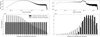 |
Fig. B.1 Histogram of the number of species in the composite synthetic spectra. The black bars correspond to the initial molecular composition, while gray dashed bars correspond to the number of detectable species after taking into account a varying noise distribution. Left: "Unconstrained" subset of synthetic spectra with a randomly selected molecular composition. Right: "Recipe" subset of data with a constrained molecular composition. The noise distribution is given on the top panel for each subset. |
Appendix C Monte Carlo dropout results
Table C.1 lists the detection probabilities from Sect. 4.5. Table C.2 lists the detection probabilities from Sect. 4.8.
Monte Carlo dropout results for the impact of the noise level on the detection probability.
Monte Carlo dropout results for the EMIR setups.
Appendix D Principle of the occlusion analysis
We use here the occlusion analysis as a model interpretation technique with the aim to assess the importance of specific channels in the CNN model’s prediction. As discussed in Sect. 4.7 in detail, we perform a systematic masking (that we refer to as occlusion) small portions of the input spectrum using a sliding window. We then quantify the changes in the CNN model’s output, where significant changes imply that the masked channels contain crucial information for its decision making. Figure D.1 illustrates the principle of our occlusion analysis. The CNN model generates a prediction for the original spectrum and for the modified version in which a small window of five channels is masked. The difference between these two predictions is computed and referred to as the occlusion score. This process is repeated across the entire spectrum.
Computing the occlusion score for each windowed region, we can map the relative contribution of the spectra to the prediction. Overall, this method provides us some interpretability by highlighting which frequency ranges the model relies on most heavily. In particular, comparing the frequency ranges used by the CNN model with known molecular transitions allows us to assess whether its decision-making aligns with our expectation that it relies on physically meaningful spectral features.
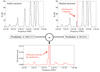 |
Fig. D.1 Principle of the occlusion analysis for the example of a CH3CN LTE model. |
Appendix E Data preparation and application of our CNN model
E.1 Preparation of the spectra
The CNN model can be easily applied to any new spectrum, regardless of the telescope specificity, resolution or setup. The CNN model can also be adapted to new observational contexts, such as a different frequency coverage, different physical properties, or a different chemical richness through transfer learning (cf. Sect. 4.8). However, to use the CNN model for a prediction, one must complete standard data reduction, such as continuum subtraction, vLSR correction and resampling to the given frequency range with a 1 MHz spectral resolution. The latter can be done using a software such as PySpecKit (Ginsburg & Mirocha 2011), CASSIS (Vastel et al. 2015), or CASA (CASA Team 2022). Noticeable gaps in the spectra or artifacts should be put to 0.
E.2 Importing the CNN model and spectra to CIANNA
The CNN model is shared according to the Apache-2.0 license, with a mandatory reference to this article, and can be found at : https://github.com/NinaK7/CNN-model-for-molecular-detection. This CNN model can be used or can be modified to be applied on new data. The test dataset (cf. Sect. 2.4) and the "typical hot core spectrum" (cf. Sect. 2.3) mentioned in this article can be found on the GitHub web page.
Our CNN model can be deployed in Python using the CIANNA API (Cornu 2025). First, the spectra must be loaded that can be done from any format (ASCII or FITS), after having pre-formatted it as discussed above in App. E.1. The input data need to be normalized according to the procedure presented in the paper, and converted to Numpy arrays compatible with the CIANNA format by the user before loading and running the trained model.
Model inference can be done on a lightweight hardware, no GPU is required for the application on a single spectrum, but the obtained performance may differ from the one from this article where we use a NVIDIA A100 GPU. In our situation, and at a computing precision of FP32C_FP32A, the inference for 2 × 10⁴ spectra made on the averaged CNN model is done in less than 1.7 seconds, i.e., ∼ 1.2 × 10⁴ spectra per second, and takes a RAM of 874 MB. The initialization of the framework in itself takes 0.30 s and the weight loading takes 0.28 s.
All Tables
Physical parameters used for the LTE models compared to literature values for hot core and hot corino sources.
Monte Carlo dropout results for the impact of the noise level on the detection probability.
All Figures
|
Fig. 1 Synthetic spectrum of a classical hot core computed from Table A.5 with a 5 km s−1 line width, a 50 mK Gaussian noise, and a zoom-in on 400 MHz. The LTE models are shown in color. The mask computed with the molecules from Table A.3 is in gray. The fake lines and absorption features are in blue and red, respectively. |
| In the text | |
|
Fig. 2 CNN architecture scheme. Input data form an example of a composite spectrum according to the three normalizations, i.e., by the maximum (top), hyperbolic tangent (center), and polynomial (bottom). Filters are applied to the data to convolve the information and produce features maps. This operation is done for each of the convolutional layers. Dense layers then combine the extracted features and learn how to label the spectra depending on the provided target. The output layer is composed of one neuron per class giving a score between 0 and 1, independent of each other. |
| In the text | |
|
Fig. 3 Loss function computed on the validation dataset and AUC values as a function of training iterations with specified minimum loss and the corresponding AUC. |
| In the text | |
|
Fig. 4 ROC curves of the molecules for which the CNN learned to detect their spectral signature. The values are computed on a [0, 1] range from the x- and y-axis. |
| In the text | |
|
Fig. 5 AUC as a function of molecules for three trainings of the multi-labeling CNN. The squares, triangles, and stars are the AUC values. The red crosses correspond to the number of spectra where the molecules are detected. |
| In the text | |
|
Fig. 6 Performance of the model as the AUC in function of line density. Color: mean AUC values for individual molecules. Black: mean global AUC value per bin. The number of spectra for AUC computation for each line density bin is specified. The line density of Sgr B2(N) observed with the 30m telescope (Belloche et al. 2013) is displayed as reference. |
| In the text | |
|
Fig. 7 Calibration curve for C2H5OH based on the number of true and false detections over the test dataset. |
| In the text | |
|
Fig. 8 Performance of the model as a function of noise. The AUC for each molecule is in color, while the average value over all species is in black. |
| In the text | |
|
Fig. 9 Detection probability (average on 1000 realizations) as a function of the line density and the noise level. The blue horizontal line and the green vertical line correspond to the line density and noise limits of our training dataset. |
| In the text | |
|
Fig. 10 Probability of detection (average on 100 realizations) for each molecule, depending on the fraction of intentionally hidden transitions. |
| In the text | |
|
Fig. 11 First maximum of the occlusion analysis score for C2H5OH. |
| In the text | |
|
Fig. B.1 Histogram of the number of species in the composite synthetic spectra. The black bars correspond to the initial molecular composition, while gray dashed bars correspond to the number of detectable species after taking into account a varying noise distribution. Left: "Unconstrained" subset of synthetic spectra with a randomly selected molecular composition. Right: "Recipe" subset of data with a constrained molecular composition. The noise distribution is given on the top panel for each subset. |
| In the text | |
|
Fig. D.1 Principle of the occlusion analysis for the example of a CH3CN LTE model. |
| In the text | |
Current usage metrics show cumulative count of Article Views (full-text article views including HTML views, PDF and ePub downloads, according to the available data) and Abstracts Views on Vision4Press platform.
Data correspond to usage on the plateform after 2015. The current usage metrics is available 48-96 hours after online publication and is updated daily on week days.
Initial download of the metrics may take a while.