| Issue |
A&A
Volume 704, December 2025
|
|
|---|---|---|
| Article Number | A172 | |
| Number of page(s) | 14 | |
| Section | Astrophysical processes | |
| DOI | https://doi.org/10.1051/0004-6361/202555849 | |
| Published online | 05 December 2025 | |
Relativistic hydrodynamics simulations of supernova explosions within extragalactic jets
1
Departament d’Astronomia i Astrofísica, Universitat de València, C/ Dr. Moliner, 50, 46100 Burjassot, València, Spain
2
Observatori Astronòmic, Universitat de València, C/ Catedràtic José Beltrán 2, 46980 Paterna, València, Spain
3
Departament de Fìsica Quàntica i Astrofísica, Institut de Ciències del Cosmos (ICC), Universitat de Barcelona (IEEC-UB), Martí i Franquès 1, E08028 Barcelona, Spain
★ Corresponding author: This email address is being protected from spambots. You need JavaScript enabled to view it.
Received:
6
June
2025
Accepted:
6
October
2025
Abstract
Context. Jets in active galactic nuclei (AGN) have to cross significant distances within their host galaxies, meeting large numbers of stars of different masses and evolution stages on their paths. Given enough time, supernova explosions within the jet will eventually happen, and they may have a strong impact on its dynamics, potentially triggering powerful non-thermal activity.
Aims. We aim to carry out a detailed numerical study to explore the dynamics of the interaction between the ejecta of a supernova explosion and a relativistic extragalactic jet.
Methods. By means of relativistic hydrodynamics simulations using the code RATPENAT, we simulated the jet-ejecta interaction in two different geometries or scenarios: a two-dimensional, axisymmetric simulation, and a three-dimensional one, which includes the orbital velocity of the exploding star. In both scenarios, the supernova ejecta is located within the jet at a distance of ∼1 kpc from the central black hole, which is the spatial scale on which these events are most likely.
Results. Although initially filling a region much smaller than the jet radius, the ejecta expands and eventually covers most of the jet’s cross-section. The expansion is enhanced as more energy from the jet is converted into kinetic and internal energy of the ejecta, which also favours the ejecta disruption, all of this occurs on timescales of ∼104 yr. Although a complete numerical convergence of the results is unattainable given the subsonic, turbulent nature of the interaction region, the simulations are consistent in their description of the gross morphological and dynamical properties of the interaction process.
Conclusions. At the end of the simulations, the supernova ejecta already partially mixed with the relativistic jet. The results also suggest that the jet-ejecta interaction may be a non-negligible non-thermal emitter. Moreover, due to efficient mixing, the interaction region can be a potential source of ultra-high-energy cosmic rays of heavy composition.
Key words: relativistic processes / supernovae: general / galaxies: active / galaxies: jets
© The Authors 2025
 Open Access article, published by EDP Sciences, under the terms of the Creative Commons Attribution License (https://creativecommons.org/licenses/by/4.0), which permits unrestricted use, distribution, and reproduction in any medium, provided the original work is properly cited.
This article is published in open access under the Subscribe to Open model. This email address is being protected from spambots. You need JavaScript enabled to view it. to support open access publication.
1. Introduction
Being launched from the surroundings of a supermassive black hole (SMBH) at the centre of an active galactic nucleus (AGNs), relativistic extragalactic jets are collimated outflows that propagate through the galactic medium within their first kiloparsecs (Begelman et al. 1984; Blandford et al. 2019). The inner galactic regions are known to contain large amounts of gas and stars and related objects (e.g. Burbidge 1970; Kauffmann et al. 2003; Hubbard & Blackman 2006; Shao et al. 2010). The interaction between the jet and such objects is unavoidable and has been well studied, with the focus either on dynamical (e.g. Komissarov 1994; Bosch-Ramon et al. 2012; Perucho et al. 2014, 2017; Anglés-Castillo et al. 2021) or radiative effects (e.g. Barkov et al. 2010; Bosch-Ramon et al. 2012; Araudo et al. 2013; de la Cita et al. 2016; Fichet de Clairfontaine et al. 2025). Very close to the SMBH, it has been proposed that this kind of interaction and its resulting emission often occur as short and relatively frequent events (e.g. Aharonian et al. 2017; del Palacio et al. 2019; Zajacek et al. 2020; Kurfürst et al. 2025), while further downstream of the jet the interaction timescales can be much longer and several events may coexist (e.g. Wykes et al. 2015; Torres-Albà & Bosch-Ramon 2019). Unless the obstacle rest mass is large or the jet power is low, gas clouds and stellar-wind envelopes that interact with the jets can be completely disrupted (Bosch-Ramon et al. 2012), in which case the mass of the object determines the maximum energy dissipated by the interaction, and the jet spatial scale characterises the overall evolution time (e.g. Khangulyan et al. 2013).
Among the object types that can face extragalactic jets, the ejecta produced by supernova (SN) explosions is perhaps one of the least studied ones (e.g. Blandford & Koenigl 1979; Fedorenko & Courvoisier 1996; Bednarek 1999). However, core-collapse SN explosions occurring inside jets in galaxies with non-negligible star formation can lead to significant non-thermal emission, as proposed, for example, in Vieyro et al. (2019). A similar situation regardless of the galaxy star-formation rate can also be realized when type Ia (thermonuclear) SN explosions interact with the jet (Torres-Albà 2019). Although the occurrence of these events is low1, the duration of such an interaction is long2. Therefore, given that most of SN explosions occur within a few kiloparsecs from the centre of galaxies, Bosch-Ramon (2023) concluded that up to ∼10% of jetted AGNs may host a jet-SN interaction at some stage of their evolution. Since no strong qualitative differences are expected between core-collapse and thermonuclear supernovae (SNe), both star-forming and non-star-forming jetted AGN are worth considering when studying these events, with the most likely height scale (jet length from the SMBH to the interaction site) being between several hundred and 1000 parsecs (see Bosch-Ramon 2023 and references therein).
Initially, the SN ejecta expands freely until its expansion is stopped in the upstream jet direction when the ejecta and jet ram pressures are balanced. At this point, the thermodynamical properties and dynamics of the ejecta become dominated by the jet impact. The expansion rate of the shocked gas is then expected to accelerate, and previous work on jet-cloud interactions suggests that the shocked ejecta may be disrupted and mixed with the jet flow (see Bosch-Ramon 2023 and references therein). For instance, this was suggested by two-dimensional (2D) axisymmetric simulations presented in Vieyro et al. (2019), but the simplified geometry and low resolution of the simulations prevented arriving at strong conclusions. Moreover, the fact that the star is orbiting the centre of the galaxy can lead to some anisotropy in the jet-SN interaction even if the associated velocity is small with respect to that of the jet, which adds to the limitations of 2D simulations. More detailed and realistic simulations are also needed to better understand non-thermal processes in these interactions.
Motivated by the lack of thorough dynamical studies of extragalactic jet-SN ejecta interactions and as a first step, we investigated this scenario using numerical simulations in the context of relativistic hydrodynamics (RHD). Simulations including a magnetic field will be presented in future work. Two different cases were considered here: as a first exploration and for computational time purposes, we first ran 2D axisymmetric RHD simulations, followed by three-dimensional (3D) runs. We adopted two different numerical resolutions to study the interaction scenario (1) with the largest accuracy attainable with affordable supercomputing resources, and (2) in the largest spatial and temporal domains, without compromising the numerical consistency of the results. The paper is structured as follows: in Sect. 2, we present the physical scenario in more detail, and in Sect. 3 we describe the 2D and 3D RHD simulation runs for this study. In Sect. 4, we present the results obtained for the different cases considered, and finally in Sect. 5 we discuss our results and give our conclusions.
2. Jet and supernova ejecta properties
We consider that the interaction occurs at a distance of 1 kpc from the SMBH, when the jet is completely developed, its radius is ∼100 pc, and the stellar density is still large. For simplicity, we assumed an opening angle of 0.2 radian, which implies a jet radius of Rj = 100 pc. The simulations are set up at a point in which the SN is large enough to be properly resolved in terms of cell numbers per diameter. Our setups are, nevertheless, spatially scalable in the sense that the jet radius determines the jet ram pressure, so adopting a narrower (wider) jet would imply the interaction being located proportionally farther from (closer to) the SMBH. The simulations can also be scaled to other jet-ejecta interaction scenarios in which, ceteris paribus, the jet-ram pressure-to-obstacle mass ratio is the same. Thermal cooling may break this symmetry, but this effect can be neglected given the involved low densities, high temperatures and relatively short evolution times at the considered jet scales. Finally, following Bosch-Ramon (2023), we adopted an intermediate jet power within typical AGN jet values, Lj = 1044 erg s−1.3 On the one hand, this power is high enough to accelerate ultra-high-energy cosmic rays (UHECRs) at the jet-SN interaction region, and, on the other hand, low enough to increase the odds of these events happening in the local Universe (Bosch-Ramon 2023).
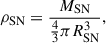
The SN ejecta initial conditions have been characterized in a simplified manner, given the difference in spatial scales involved, to avoid an excessive computational demand. Therefore, we modelled the initial SN state as a uniform highly pressured and dense bubble at rest, with a total internal energy similar to the typical kinetic energy of an SN ejecta, ESN = 1051 erg (Leahy 2017), and a mass of MSN = 2 M⊙, between those released by thermonuclear (SN Ia) and core-collapse SNe. The initial ejecta density is thus
 (1)
(1)
where RSN is the initial SN ejecta radius, which is fixed in our simulations to a given initial value. The value of RSN depends on the expected maximum upstream expansion of the ejecta as measured from the SN initial location. Under these conditions, the initial expansion speed can be estimated as  km s−1. The ejecta will expand at this speed in all directions until the jet ram pressure becomes significant and upstream expansion decelerates.
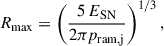
From the very beginning, the jet-ejecta interaction develops a bow-shaped structure made of shocked jet flow common in jet-obstacle interactions (e.g. Komissarov 1994; Bosch-Ramon et al. 2012). The expected maximum expansion point in the jet upstream direction is located at a distance from the SN explosion origin that can be approximated by imposing pressure balance between the shocked jet and ejecta:
 (2)
(2)
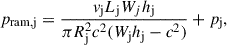
where pram, j is the jet-ram pressure:
 (3)
(3)
where pj is the jet pressure, vj the jet flow speed, and Wj and hj are the jet Lorentz factor and specific enthalpy, respectively (where hj = c2 + εj + pj/ρj, with εj = pj/(Γ − 1) being the specific internal energy and Γ the adiabatic index). Beyond this moment, the ejecta evolution becomes dominated by the jet ram pressure. The initial ejecta radius in the simulation is taken to be a small fraction of Rmax, that is, RSN = fR Rmax with fR ≪ 1, to allow us to start following the evolution of the ejecta while it is still well within its free expansion phase.
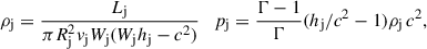
The Lorentz factor of the jet is taken as Wj = 2 (vj ≈ 0.866 c) and the specific enthalpy as hj = 1.1 c2, so that the unshocked jet density and gas pressure can be derived from
 (4)
(4)
to give ρj ≈ 6 × 10⁻³⁰ g cm−3, pj ≈ 2 × 10⁻¹⁰ dyn cm−2. Finally, with the jet-flow velocity fixed, the jet ram pressure and the maximum expansion size of the SN ejecta can be established: pram, j ≈ 1.8 × 10⁻⁸ erg cm−3, Rmax ≈ 11 pc. Then, at an expansion speed of ∼104 km s−1, the ejecta would reach this point after ∼103 yr.
Both in 2D and 3D, two different initial SN radii were simulated: 10 (S1) and 5 (S2) times smaller than the maximum expansion radius (i.e. fR = 0.1, 0.2); thus we have RSN = 1.1, 2.2 pc. The number of cells per initial SN radius is the same in both simulations, so the effective spatial resolution is doubled in S1 with respect to S2. Furthermore, we introduced an ejecta velocity of 200 km s−1 perpendicular to the jet, mimicking the orbital velocity of the progenitor star and therefore introducing an asymmetry in the system.
Despite the fact that the ejecta initial expansion speed is ∼50 times larger than the orbital one, the global structure of the shocked ejecta can develop large asymmetries as it evolves. The grid surrounding the initial SN bubble was filled with a homogeneous jet flow.
Regarding the gas composition, we assumed, for both the SN ejecta and the jet, a neutral electron-proton gas with a leptonic mass fraction Xe = me/mp ≈ 5.5 × 10⁻⁴, yielding an effective mass per particle meff ≈ mp/2. This is a reasonable plasma prescription if the jet has been significantly mass-loaded within the inner regions of the galaxy, which is expected (Perucho et al. 2014; Anglés-Castillo et al. 2021). The initial SN ejecta density was determined by RSN, 1.1 pc in S1 and 2.2 pc in S2, resulting in ρSN = 2.4 × 10⁻²³ g cm−3, and 3 × 10⁻²⁴ g cm−3, respectively. Finally, the gas temperature was computed using T = meff p/kB ρ for both jet and ejecta (with the initial ejecta pressure derived from ESN and RSN). Thus, the ejecta temperature is TSN ≈ 109 K at the start of the simulation; in the unshocked jet, the temperature is to Tj ≈ 2 × 10¹¹ K.
3. Simulations
To run the simulations, we used a finite-volume code, which solves the RHD equations in conservative form by means of high-resolution shock-capturing methods (HRSCs). We used its OpenMP version in cylindrical coordinates for the axisymmetric 2D simulations, while we used the hybrid MPI + OpenMP version (RATPENAT; Perucho et al. 2010) for the 3D simulations in Cartesian coordinates.
In 3D Cartesian coordinates, the conservation equations in c = 1 units can be written as follows:
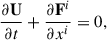 (5)
(5)
where the state vector U are:
 (6)
(6)
and the vectors of fluxes Fi is
 (7)
(7)
with i, j = 1, 2, 3, and summation over repeated indices implicit. The variables D, De, Si, and τ are, respectively, the total and leptonic rest-mass densities, the momentum density in each spatial direction, and the energy density (without the rest-mass energy density), defined in the laboratory frame, and are related to the quantities in the local rest-frame of the fluid as:
 (8)
(8)
where ρ and ρe are the total and leptonic densities, vi the components of the velocity of the fluid, W the Lorentz factor (W = (1 − vivi)−1/2), p the gas pressure, and the specific enthalpy is defined in c = 1 units as
 (9)
(9)
The code uses the Synge equation of state (Synge 1957), which includes protons and electrons as a mixture of relativistic Boltzmann gases. Finally, we used a tracer, f, which gives the jet-mass fraction, and allowed us to trace the mixing between jet (f = 1) and SN ejecta (f = 0) materials.
3.1. 2D axisymmetric simulations
We first ran 2D axisymmetric simulations in which we set up a uniform, highly pressured and dense bubble of gas, which corresponds to the SN ejecta, surrounded by a homogeneous relativistic jet flow moving in the Z-direction, similarly to what was implemented in previous works (e.g. Vieyro et al. 2019). Figure 1 zooms into the region around the SN ejecta during the free expansion phase. The figure shows a still-spherical core of the remnant of the shocked ejecta and the development of a downstream-elongated tail. Upstream, a bow shock separates the region of interaction from the undisturbed homogeneous jet flow.
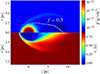 |
Fig. 1. Snapshot of jet-SN interaction during the initial phase to illustrate the setup of the 2D axisymmetric simulations. Upper half: Rest-mass density, ρ. Lower half: Axial velocity, vz. The dashed white line gives the jet-mass fraction contour for the tracer value f = 0.5. The jet flow is filling the grid but in the ejecta region and propagates from left to right. |
In these 2D simulations, we used cylindrical coordinates and assumed axisymmetry. Accordingly, the left and right boundaries of the Z-axis are defined with an inflow and outflow condition, respectively, whereas in the radial direction, the conditions are a reflection of the symmetry axis and outflow at the outermost boundary.
In the first of our simulations, S1 (RSN = 1.1 pc), the dimensions of the grid are Lr × Lz = 96 RSN × 192 RSN, with 768 × 1536 cells, resulting in a resolution of eight cells/RSN. In the case of S2 (RSN = 2.2 pc), the dimensions of the grid are Lr × Lz = 80 RSN × 120 RSN, with 640 × 960 cells, and the same number of cells per RSN. The ejecta is initially centered on the axis, at one fourth of the grid length (i.e. z = Lz/4). We ran the simulations on 32 cores in the supercomputing facility Lluís Vives at Universitat de València.
3.2. 3D simulations
The physical setup is very similar to the one we used in our 2D simulations, including numerical resolution. As a main difference, we included the orbital velocity (vorbx = 200 km s−1) of the progenitor star around the galactic centre. The geometry of the grid is now Cartesian and is defined with a volume (X, Y, Z) [ − 50, 50] RSN × [0, 100] RSN × [ − 50, 50] RSN (i.e., Lx = Ly = Lz = 100 RSN) and 8003 cells for simulation S1 (RSN = 1.1 pc), and (X, Y, Z) [ − 40, 40] RSN × [0, 80] RSN × [ − 40, 40] RSN (i.e., Lx = Ly = Lz = 80 RSN) and 6403 cells for S2 (RSN = 2.2 pc). Those numbers result in a resolution of eight cells/RSN in both cases, the same as that used in the 2D simulations. We also ran the same 3D simulations, but for an initial ejecta at rest, to calibrate the effect of the initial ejecta motion perpendicular to the jet; the results of this simulation are shown in Appendix A.
The initial SN ejecta is centred in the XZ plane and at a distance of Ly/5 from the left boundary along the Y-axis in S1 and Ly/8 in S2. The jet propagates along the Y-axis and fills the rest of the grid. Except for the left boundary of the Y-axis, where we injected the jet flow, all other boundaries of the numerical box are set with an outflow condition. The 3D simulations were also run on Lluís Vives, using either 128 or 256 cores. Table B.1 in the appendix shows the parameter values adopted for the simulations.
4. Results
4.1. Simulation S1
This simulation focuses on the evolution of a SN explosion, in which an ejecta of 2 M⊙ and 1051 erg initially fills a spherical region with radius 1.1 pc (∼0.1 Rmax). In the following sections, we first present the results for the 2D axisymmetric simulation, and then those obtained for the 3D one.
4.1.1. 2D axisymmetric case
We show the evolution of the ejecta developing within the jet flow in Fig. 2, where the rest-mass density and axial-flow velocities are shown in the upper and lower halves, respectively. A solid black line in the velocity plots indicates the jet-mass fraction at 0.5. The top left panel shows a snapshot after 1600 yr of evolution, about the end of the free expansion phase of the ejecta, when it has expanded to a radius close to the maximum expected one, Rmax, as given by the analytical calculation (Eq. 2). At the same time, the bow shock in the jet is fully developed and the jet flow is heated and compressed through the discontinuity (up to a density of ∼4 × 10⁻²⁹ g cm−3). A backward shock (in the ejecta reference frame) detaches from the jet-ejecta impact point and starts to cross the (otherwise still homogeneous) ejecta (red-orange transition). Downstream, the tail formed with ejecta material around the symmetry axis has already reached the outer boundary. The top right panel shows a snapshot at t = 2300 yr. The backward shock (red/orange transition) continues its propagation through the initially freely expanding ejecta, compressing it and heating it up. It thus serves as a means to transfer kinetic energy from the jet into internal energy through the shocked ejecta. The heating favours the lateral expansion. As a consequence, the shocked-jet/ejecta boundary (see the black contour in the lower half panel) greatly increases its cross-section, stops the advance in the upstream direction, and develops Rayleigh-Taylor instabilities.
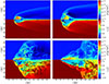 |
Fig. 2. Time evolution of rest-mass density (upper half panels) and axial velocity (lower half panels, mirror of the upper panels) for S1 in 2D. The black lines give the contour of the jet-mass fraction for the tracer value f = 0.5. The jet is propagating from the left to the right. Top left: t ≈ 1600 yr from the start of the simulation; top right: t ≈ 2300 yr; bottom left: t ≈ 3000 yr; bottom right: t ≈ 3800 yr. |
The bottom left panel shows a snapshot at t = 3000 yr. At this point, the remnant of the ejecta has been almost stripped by the shocked jet flow and its material dragged downstream and mixed under the action of Rayleigh-Taylor and Kelvin-Helmholtz instabilities. The cross-section of the shocked jet/ejecta boundary now reaches ∼60 pc and the jet bow shock touches the radial boundary of the numerical grid. The instability growth leading to the ejecta remnant disruption is fast even in this axially symmetric 2D case, as suggested by previous works studying similar scenarios, such as Bosch-Ramon et al. (2012), Perucho et al. (2017), and Vieyro et al. (2019). In the case of Vieyro et al. (2019) in particular, in which the interaction of an SN ejecta with a jet was specifically studied, the results qualitatively match those found here. However, the resolution of the S1 2D simulation is ten times higher than in the one adopted in Vieyro et al. (2019) (in which the initial ejecta radius was ∼Rmax, among other more minor differences), allowing for a much more nuanced description of the development of instabilities. This can be seen comparing Fig. A.1 of that work with our Fig. 2. Those simulations also addressed a much more unlikely type of event, taking place much closer to the base of a more powerful AGN jet, so the present results are more relevant for the jetted AGN population as a whole.
The bottom right panel shows the situation at the end of the simulation (t = 3800 yr), with the disrupted shocked flow made of mixed jet and ejecta materials being advected down out of the grid but for chunks of shocked ejecta around the axis (probably an artefact of the axisymmetry of the simulation) where the density remains around 10−25 − 10−26 g cm−3, that is, two-to-three orders of magnitude smaller than the initial bubble density, and four or five orders of magnitude denser than the original jet flow. The mixed jet and ejecta material is expected to mass load the whole jet downstream, outside the grid, forming a tail of turbulent flow somewhat slower than the jet that is likely to homogenise on level of the jet scale height. At this point, it is interesting to note that the interaction of the jet with the SN ejecta studied in this simulation represents a transient episode in the jet’s lifetime since the jet injects amounts of energy and mass equal to those delivered by the SN ejecta in about one and 104 yr, respectively (the latter being similar to the overall interaction timescale).
4.1.2. 3D case
Figure 3 shows six snapshots of the density in the XY plane at the middle point of the Z-axis (z = 0). The snapshots show the density distribution on that plane at different times during the simulation, ordered from top left to bottom right. The chosen snapshots correspond to the times shown in Fig. 2 (t ≃ 1600, 2300, 3000, 3800 yr) plus an initial and a final snapshot (t ≃ 180 yr and 4700 yr, respectively). During the initial phase (first two panels, t ≤ 1600 yr) the structure of the ejecta is fairly symmetric (with Rayleigh-Taylor instabilities developing at the shocked jet/ejecta boundary) and resembles the 2D simulation, although the 3D nature of the flow (introduced by the initial perpendicular velocity vorbx given to the ejecta) prevents the tail of ejecta material around the Y-axis (see first panel of Fig. 2) from being formed.
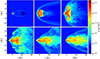 |
Fig. 3. Time evolution of rest-mass density for S1 in 3D, with six 2D cuts in the XY plane at z = 0. The jet is propagating from the left to the right. Top left: t ≈ 180 yr; top middle: t ≈ 1600 yr; top right: t ≈ 2300 yr; bottom left: t ≈ 3000 yr; bottom middle: t ≈ 3800 yr; bottom right: t ≈ 4700 yr. |
Three-dimensional effects become more apparent as time goes on. In the third top panel of Fig. 3 (t ≃ 2300 yr), one already sees evidence of turbulent mixing (driven by a combination of Rayleigh-Taylor and Kelvin-Helmholtz instabilities) in the whole region within the jet shock, which has widened up extending over most of the grid and reaching a scale of ∼100 pc, while the shocked ejecta is being quickly disrupted. All this happens significantly faster than in 2D (compare the panels at t ≃ 2300 yr in Figs. 2 and 3) because of the higher dimensionality and consequent enhanced instability growth.
As in the 2D case, beyond 3000 yr (bottom panels of Fig. 3) the stripped material from the shocked ejecta starts to be dragged downstream as the shocked region narrows. At t ≃ 3800 yr (the last snapshot comparable with the 2D case), the overall structure of the shocked flow in the two simulations is similar.
Figure 4 shows cuts of the 3D box in the XY plane at z = 0 for the temperature (upper half panels) and tracer (jet mass fraction, lower half panels) for the same times as those in Fig. 3. Regarding temperature, the ejecta cools down from the initial ∼109 K to ≤108 K during the free expansion phase, whereas it reheats dramatically in its shocked phase. The upper panels show the propagation of the initial-jet-driven shockwave through the cloud and the resulting reheating of the shocked ejecta by two orders of magnitude, reaching temperatures of ∼1010 K. In contrast, in the much more diluted shocked jet gas the temperature rises up to ∼1012 K. The highest temperatures are reached where the jet shock surface is nearly perpendicular to the undisturbed jet flow.
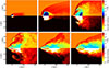 |
Fig. 4. Time evolution of temperature (upper half panels) and tracer of jet-mass fraction (lower half panels) for S1 in 3D, with 6 2D cuts in the XY plane and at z = 0; the lower half corresponds to the same region shown in the upper half, but inverted with respect to the axis on x = 0. The jet is propagating from the left to the right. Top left: t ≈ 180 yr; top middle: t ≈ 1600 yr; top right: t ≈ 2300 yr; bottom left: t ≈ 3000 yr; bottom middle: t ≈ 3800 yr; bottom right: t ≈ 4700 yr. |
The lower halves of the panels in Fig. 4 show the jet-mass fraction. The jet material engulfed by the shocked ejecta during the development of the Rayleigh-Taylor instabilities (t ≥ 1600 yr) favours rapid mixing. At the same time, the development of Kelvin-Helmholtz instabilities at the shocked jet-ejecta interface (already visible at the back of the ejecta beyond 1600 yr) enhance the mixing rate while the jet bow shock reaches its largest cross-sectional size. Due to the much higher density of the ejecta, the jet-mass fraction remains very low in the innermost regions of the interaction structure. Nevertheless, the strong mixing observed in the widening two-flow boundary layer (black-red-yellow-white transition) indicates that the jet and the ejecta will mix completely further downstream. Strong mixing is also visible in the remains of the ejecta that still survive at the end of the simulation.
Finally, Fig. 5 shows the 3D distribution of the shocked structure density in code units, at t ≈ 3000 yr. In the image, the jet flow propagates from left to right, along the Y-axis. We show the surfaces that trace the distribution of the expanded, shocked SN ejecta in red and green, whereas the dark blue shows more compact regions and the light red shows how a partly transparent surface traces the shocked jet layer surrounding the shocked ejecta. The snapshot time corresponds to the maximum shocked structure expansion during the simulation, which coincides with the disruption of the shocked SN ejecta.
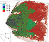 |
Fig. 5. Coloured surfaces of rest-mass density 3D distribution, in code units, for the evolved structure of simulation S1 at t ≈ 3000 yr, corresponding to the bottom left panel of Fig. 3. The axis of the jet is in the middle of the XZ plane, and the latter propagates along the Y-axis (triad visible in the bottom left of the image) and from left to right; the surfaces show the shocked ejecta interacting with the jet flow, while the nearly transparent red layer surrounding the shocked ejecta outlines the shocked jet region. |
4.2. S2 simulations
In the S2 set of simulations, the jet and ejecta properties are the same as in S1, except for RSN, the initial radius of the supernova ejecta, which is now 2.2 pc. Since the number of cells for the initial radius is still 8, as in S1, the resolution is effectively twice lower in S2, and its results are slightly different from those of S1.
4.2.1. 2D axisymmetric case
Figure 6 shows four snapshots of the rest-mass density (upper half panels) and the axial velocity (lower half panels) for the S2 2D simulation at times t ≃ 1500, 2200, 2900, 4000 yr. Taking into account that the SN ejecta expands at a speed of ∼0.01 pc/yr, these correspond approximately to those of Fig. 2; the SN ejecta is initially more diluted and colder in S2, so the phase of ejecta-free expansion captured by the simulation is slightly shorter than in S1 (about 100 yr). In contrast to S1, in which the total disruption of the SN ejecta occurs between 2300 and 3000 yr (second and third panels of Fig. 2), for S2 this happens between t = 2900 and 4000 yr (third and fourth panels of Fig. 6). Most of the mixing takes place during this period, and the maximum lateral expansion of the shocked flow occurs ∼4000 yr after the start of the simulation, versus ∼3000 yr in S1. Despite this shift caused by the lower resolution of S2, which slows down the development of instabilities, the evolution of the system is qualitatively the same as that observed in S1.
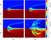 |
Fig. 6. Same as Fig. 2, but for 2D axisymmetric S2 simulation. Top left: t ≈ 1500 yr; top right: t ≈ 2200 yr; bottom left: t ≈ 2900 yr; bottom right: t ≈ 4000 yr. |
4.2.2. 3D case
Figure 7 shows cuts of the rest-mass density box in the central plane of the Z coordinate (z = 0) for the 3D S2 simulation. The corresponding times are comparable to those in Fig. 3. As in the case of S1, the break of symmetry introduced by the transversal motion of the SN ejecta becomes evident during the maximum expansion phase of the shocked flow. Similarly to the 2D simulations, the total disruption of the SN ejecta is delayed so that it occurs between 2900 and 4000 yr (between t = 2300 and 3000 yr in S1). During this phase of disruption, stripped material from the SN ejecta resist the jet-ram pressure and propagate up to large distances (see the fifth and sixth panels of Fig. 7) before being completely mixed. This also happens in S1, but earlier (see fourth panel of Fig. 3). Overall, simulations S1 and S2 follow a qualitatively similar evolution despite the differences introduced by the initial condition, effective resolution and grid size. Interestingly, the larger grid of S2 allows us to follow the evolution of the jet-ejecta interaction for longer times (although the state of the flow in the last frame, t ≃ 4700 yr, would be equivalent to a time between 3000 and 3800 yr in S1).
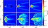 |
Fig. 7. Same as Fig. 3, but for S2 in 3D. Top left: t ≈ 350 yr; top middle: t ≈ 1500 yr; top right: t ≈ 2200 yr; bottom left: t ≈ 2900 yr; bottom middle: t ≈ 4000 yr; bottom right: t ≈ 4700 yr. |
Figure 8 shows six slices of the temperature (upper half panels) and jet mass fraction (lower half panels) at different simulation times comparable to those in Fig. 4. The distribution and values of temperature in the post-shock material along the simulation are similar to those in S1. The distribution of the tracer at long times (t ≥ 4000, comparable with times t ≥ 3000 in S1) allows us to conclude that although the smaller resolution in S2 delays the development of instabilities, it is more effective in stripping and mixing the ejecta material once they develop to non-linear amplitudes.
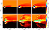 |
Fig. 8. Same as Fig. 4, but for S2 in 3D. Top left: t ≈ 350 yr; top middle: t ≈ 1500 yr; top right: t ≈ 2200 yr; bottom left: t ≈ 2900 yr; bottom middle: t ≈ 4000 yr; bottom right: t ≈ 4700 yr. |
Finally, Fig. 9 shows the equivalent of Fig. 5 for S2, after 4700 yr from the start of the simulation. Again, the image shows a qualitatively similar picture to that resulting from S1, with dense knots triggering small-scale interactions as the shocked ejecta expands and gets disrupted. Beyond this region, efficient mixing with the shocked jet gas is also observed, involving scales that reach the order of the jet radius.
4.3. Maximum upstream expansion
In Sect. 3, we give an analytical estimate of the position of the equilibrium point between the ejecta and jet ram pressures, as measured from the SN original location, Rmax ≃ 11 pc. Figure 10 shows the evolution of the position of the jet bow shock, Rbs, with time along the symmetry axis of the initial ejecta, for the different simulations: S1 (left), S2 (right), 3D, and 2D for different resolutions (half and double of the reference value). The shock position is defined as the first jump in pressure met along the axis.
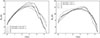 |
Fig. 10. Time evolution of jet bow-shock location in S1 (left panel) and S2 (right panel) in 2D and 3D. For the 2D simulations, the calculation is done for three different resolutions: same resolution as the 3D simulation, resolution/2 (i.e. number of cells/2) and resolution ×2 (i.e. number of cells ×2). |
The curves in the figure show a fast initial rise of Rbs, which corresponds to the ejecta-free expansion phase for all the studied cases. At t ∼ 1000 yr, the jet-bow-shock location reached values close to 10 pc. Its displacement slows down, but it keeps advancing upstream up to values well beyond the analytical estimate: Rbs ≈ 13 pc in 3D and ≈15 pc in 2D for S2; Rbs ≈ 16 pc in 3D and ≈18 pc in 2D for S1 (the 2D simulations present an acceptable agreement for the different resolutions). Eventually, the shock starts to recede as the shocked ejecta is pushed downstream of the jet.
In all cases, the maximum of Rbs is achieved 3000 − 4000 yr after the beginning of the simulations, much later than the analytical estimate of ∼1000 yr. This long delay, together with the large values achieved by Rbs can be understood, beyond the intrinsic complexity of the real jet-ejecta interaction, by considering the following two facts. First, the analytical estimate for the time needed to reach the maximum expansion assumes a constant expansion speed (equal to the initial one), without taking into account deceleration down to zero when equilibrium is reached. Second, the estimate of the position of the jet-bow-shock location is purely 1D and ignores the fact that since the ejecta has a finite radius and the jet flow is deflected laterally at the bow shock, there is a drop in the effective ram pressure exerted on the ejecta material.
The density in the shocked ejecta decreases with time (and hence its inertia) and the jet starts to push the ejecta remnant downstream in an accelerated manner. At t ≃ 5000 yr, the shocked jet-ejecta structure crosses the initial centre of the SN explosion (bottom right panels of Figs. 3 and 7), which is also indicated in Fig. 10 by the negative values of the position of the jet bow shock.
4.4. Dynamics
Entropy is a good indicator of the changes suffered by the interacting flows as they evolve. Ignoring logarithms and constants, we define the (specific) entropy as s = Tρ−2/3 (see, e.g. Lloyd-Davies et al. 2000). Figure 11 shows the average of specific entropy for the 3D simulations S1 and S2 over the domain Σ = [ − 2.5, 2.5] RSN × [ − 2.5, 2.5] RSN of the XZ plane along the Y-axis and normalised to the jet averaged entropy, for different evolution times. Restricting the averaging to Σ allows us to focus on the evolution of the entropy within the central region of the SN ejecta. The specific entropy of the ejecta material, initially small compared with that of the jet, rises with time as the ejecta is swept by the backward shock and turbulence develops. At the same time, the ejecta remnant moves downstream dragged by the jet flow.
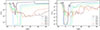 |
Fig. 11. Specific entropy (normalised to the jet entropy) averaged over domain, [ − 2.5, 2.5] RSN × [ − 2.5, 2.5] RSN of the XZ plane around the jet axis for the 3D simulations; six time steps from S1 (left panel) and S2 (right panel) are shown to accurately follow the dynamical evolution of the ejecta. |
We also studied the evolution of the total thermal energy density, u = ρ ε c2 (Γ W2 + 1 − Γ), the kinetic energy density, ek = ρ c2 W (W − 1), the density D = ρ W, in the lab frame, and the axial velocity, vy, at the right boundary of the grid through which the shocked flow leaves the computational domain. We show the results in Fig. 12. The values of ek, u, D, and vy are normalised to the background jet ones. After an initial drop caused by a rarefaction wave formed downstream of the ejecta, both quantities increase at the right boundary as the jet-ejecta interaction evolves and the shocked flow is advected by the jet out of the grid. The increase in ek is associated with the ejecta mass incorporated to the jet, whereas the increase in u is driven by shock heating (see Figs. 4 and 8). The right panel of the figure shows how the right-boundary-averaged D initially rises while vy drops. However, vy grows again due to acceleration once the ejecta has been disrupted and pushed by the jet after ∼3000 and 4500 yr in S1 and S2, respectively. The delay observed in S2 with respect to S1 again indicates that a higher resolution slightly increases the pace of the dynamical processes. The value of vy becomes mildly relativistic at the end of the simulations (∼0.65 − 0.75 c).
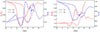 |
Fig. 12. Time evolution in 3D case of rest-mass density in the lab-frame, D; kinetic ek and internal, u, energy density (normalised to the jet values); and velocity, vy, in vj-units, averaged over the XZ plane at the outflow boundary of the Y-axis for S1 (solid lines) and for S2 (dashed lines). |
5. Discussion and conclusions
Our simulations show that a SN explosion can strongly mass load a relativistic jet on a timescale of ∼104 yr, which is consistent with the analytical estimate given in Vieyro et al. (2019) in the present scenario. This timescale is of the order of the interaction height in the jet over c, which gets shorter for more powerful jets (less common) and longer for weaker jets (more common). As noted in Bosch-Ramon (2023), the fraction of jetted AGNs hosting an interaction with a SN should be of the order of the interaction duration times the SN rate within the jet.
There are several effects of the jet-ejecta interaction that are worth mentioning: producing temporary jet deceleration and generation of transient inhomogeneities in velocity along the jet; enriching the outflow with metals that are carried on to the host cluster of the active galaxy (e.g. Kirkpatrick et al. 2009; Simionescu et al. 2010; Choi et al. 2020) or can be accelerated to ultra-high energies (Bosch-Ramon 2023); and triggering potentially detectable non-thermal emission as a consequence of the conversion of jet kinetic energy into (non-thermal) internal energy at shocks and turbulent regions (Vieyro et al. 2019).
Regarding jet mass-load, the mean rate during the simulation time is of a few times 10−4 M⊙ yr−1, taking into account the simulation timescale and the initial SN ejecta mass, which can be compared to the mass injection rate of the jet considered, ∼6 × 10⁻⁴ M⊙ yr−1. Although we modelled it as a simple electron-proton gas, the ejecta is largely made of heavy nuclei, which will mix with the jet flow as it propagates out of the galaxy. These situations can thus add non-negligible amounts of heavy metals downstream of a SN explosion to those brought by the jet due to regular mass load (e.g. entrained galactic gas, stellar winds, and accretion disc matter); the SNe may even dominate the content of heavy elements in the jet termination regions.
The simulated mass-loaded jet bulk flow features a transitory deceleration, which, for the typical parameters adopted here, can affect the whole jet cross-section. In this context, clumps of heavier material from the disrupted ejecta would be advected along the jet for a distance, with upstream, faster jet flow catching up these slower regions. The affected jet region would eventually become diluted in the jet flow while propagating towards the jet-termination region –hotspot– in Fanaroff–Riley type-II (FRII) radio galaxies, or into the surrounding plume filled by jet-ambient mixed flow in the case of FRIs.
The jet-ejecta interaction was simulated in 2D and 3D, and for different spatial resolutions. The simulations follow a qualitatively similar evolution, which suggests that in the context of (relativistic) hydrodynamical simulations, we are approaching a realistic spatial resolution level. However, although the lower resolution of S2 allowed us to extend the study to larger spatial and temporal scales, the speed of the shocked-ejecta disruption process is slightly faster when the resolution is increased, and this is likely related to the lower numerical viscosity in this case (S1). The same result is obtained when moving from 2D to 3D simulations, for which we also find that tiny perturbations of the symmetry through vorbx lead to a stronger impact of instabilities in the long-term evolution of the shocked ejecta, as seen when comparing, for example, Fig. 3 with Fig. A.2. The differences introduced by the orbital motion of the ejecta are also shown in Fig. A.1.
The simulations were run under the hypothesis that the interaction region is smaller than the jet radius, Rj, and much smaller than the jet scale height, allowing us to assume that the ejecta is immersed in a homogeneous flow. However, the scales reached by the shock, in particular in the larger grid S2 simulations, indicate that the shocked ejecta could easily reach the boundaries of the jet and strongly interact with the shear layer and the interstellar medium. This phenomenon could trigger additional shocks, and thus turbulence and mixing between the jet flow, the ejecta material and the interstellar medium gas. We will explore this scenario in upcoming work. Moreover, the presence of magnetic fields can strongly impact the dynamical and non-thermal processes involved in the jet-ejecta interaction. This possibility will also be explored by means of relativistic magnetohydrodynamical simulations, using the code LOSTREGO (López-Miralles et al. 2022).
In terms of detectability, part of the jet power is reprocessed at the shock for most of the interaction duration, that is, as long as the ejecta has not been accelerated to the jet bulk speed. Therefore, plenty of energy is likely to feed non-thermal processes. Synchrotron and inverse Compton (IC) scattering in the case of electrons would in principle be more efficient than hadronic processes, given the large scale of the interaction and diluted target fields, although specific calculations are required for a quantitative assessment. Future work will be devoted to the non-thermal consequences of the jet-ejecta interaction. Nevertheless, it is worth indicating that, unless strongly below equipartition, the shocked jet and ejecta magnetic fields make synchrotron emission strongly dominant over adiabatic or IC losses, releasing most of the energy of non-thermal electrons (and positrons) from radio to X-rays. Moreover, the spatial scales in which the jet-ejecta interaction can be more violent, ∼100 pc, translate into angular sizes of a few tens of milliarcseconds for an AGN at gigaparsec distances. This makes the scenario potentially resolvable by radio interferometric arrays, such as VLA in configuration A at ν ≥ 22 GHz, certainly for any VLBI array, and also by Hubble in nearby sources or Chandra for the nearest ones. If hadrons were also accelerated, efficient neutrino production could occur either from proton-proton (p-p) or proton-photon (p-γ) interactions, in particular for a more powerful jet with an interaction region closer to its base. Given the relatively high density of mass-loaded protons, p-p interactions could be favoured here (as suggested in Ros et al. 2020; Wang et al. 2022 in the case of TXS 0506+056 for a jet-cloud/star interaction), producing TeV to PeV neutrinos. Protons could reach even higher energies and interact with intense photon fields, allowing the production of pairs and more energetic neutrinos (> PeV) through p-γ interactions. Future studies will help us to assess the detectability of such an event with current and future neutrino facilities. Finally, the simulations show that jet-ejecta mixing is very efficient, so heavy nuclei entrained by the jet could easily reach the jet shock or the regions with strong velocity shear and turbulence downstream of the interaction, where there is a high chance of getting accelerated to ultra-high energies, as proposed in Bosch-Ramon (2023).
It is proportional to the galactic volume filled by the jet, which is roughly proportional to the square of the jet-to-galaxy radius ratio.
The duration timescale is given approximately by the jet distance from the SMBH to the interaction site over c.
Here Lj refers to kinetic power, i.e., total power excluding rest-mass energy flux.
Acknowledgments
This work has received financial support from the Spanish Ministry of Science and Innovation under grants PID2022-136828NB-C41/AEI/10.13039/501100011033/ERDF/EU and PID2022-136828NB-C43/AEI/10.13039/501100011033/ERDF/EU, through the María de Maeztu 2020-2023 award to the ICCUB (CEX2019-000918-M), and from the Generalitat de Catalunya through grant 2021SGR00679. V.B.-R. is Correspondent Researcher of CONICET, Argentina, at the IAR. We thank the anonymous referee for a constructive report that has improved the paper.
References
- Aharonian, F. A., Barkov, M. V., & Khangulyan, D. 2017, ApJ, 841, 61 [NASA ADS] [CrossRef] [Google Scholar]
- Aloy, M. A., Ibáñez, J. M., Martí, J. M., & Müller, E. 1999, ApJS, 122, 151 [Google Scholar]
- Anglés-Castillo, A., Perucho, M., Martí, J. M., & Laing, R. A. 2021, MNRAS, 500, 1512 [Google Scholar]
- Araudo, A. T., Bosch-Ramon, V., & Romero, G. E. 2013, MNRAS, 436, 3626 [NASA ADS] [CrossRef] [Google Scholar]
- Barkov, M. V., Aharonian, F. A., & Bosch-Ramon, V. 2010, ApJ, 724, 1517 [NASA ADS] [CrossRef] [Google Scholar]
- Bednarek, W. Ł. O. 1999, in Plasma Turbulence and Energetic Particles in Astrophysics, eds. M. Ostrowski, & R. Schlickeiser, 360 [Google Scholar]
- Begelman, M. C., Blandford, R. D., & Rees, M. J. 1984, Rev. Mod. Phys., 56, 255 [Google Scholar]
- Blandford, R. D., & Koenigl, A. 1979, Astrophys. Lett., 20, 15 [NASA ADS] [Google Scholar]
- Blandford, R., Meier, D., & Readhead, A. 2019, ARA&A, 57, 467 [NASA ADS] [CrossRef] [Google Scholar]
- Bosch-Ramon, V. 2023, A&A, 677, L14 [NASA ADS] [CrossRef] [EDP Sciences] [Google Scholar]
- Bosch-Ramon, V., Perucho, M., & Barkov, M. V. 2012, A&A, 539, A69 [NASA ADS] [CrossRef] [EDP Sciences] [Google Scholar]
- Burbidge, G. R. 1970, ARA&A, 8, 369 [Google Scholar]
- Choi, E., Brennan, R., Somerville, R. S., et al. 2020, ApJ, 904, 8 [NASA ADS] [CrossRef] [Google Scholar]
- de la Cita, V. M., Bosch-Ramon, V., Paredes-Fortuny, X., Khangulyan, D., & Perucho, M. 2016, A&A, 591, A15 [NASA ADS] [CrossRef] [EDP Sciences] [Google Scholar]
- del Palacio, S., Bosch-Ramon, V., & Romero, G. E. 2019, A&A, 623, A101 [NASA ADS] [CrossRef] [EDP Sciences] [Google Scholar]
- Fedorenko, V. N., & Courvoisier, T. J. L. 1996, A&A, 307, 347 [NASA ADS] [Google Scholar]
- Fichet de Clairfontaine, G., Perucho, M., Martí, J. M., & Kovalev, Y. Y. 2025, A&A, 693, A270 [NASA ADS] [CrossRef] [EDP Sciences] [Google Scholar]
- Hubbard, A., & Blackman, E. G. 2006, MNRAS, 371, 1717 [NASA ADS] [CrossRef] [Google Scholar]
- Kauffmann, G., Heckman, T. M., Tremonti, C., et al. 2003, MNRAS, 346, 1055 [Google Scholar]
- Khangulyan, D. V., Barkov, M. V., Bosch-Ramon, V., Aharonian, F. A., & Dorodnitsyn, A. V. 2013, ApJ, 774, 113 [NASA ADS] [CrossRef] [Google Scholar]
- Kirkpatrick, C. C., Gitti, M., Cavagnolo, K. W., et al. 2009, ApJ, 707, L69 [NASA ADS] [CrossRef] [Google Scholar]
- Komissarov, S. S. 1994, MNRAS, 269, 394 [CrossRef] [Google Scholar]
- Kurfürst, P., Zajaček, M., Werner, N., & Krtička, J. 2025, MNRAS, 540, 1586 [Google Scholar]
- Leahy, D. A. 2017, ApJ, 837, 36 [NASA ADS] [CrossRef] [Google Scholar]
- Lloyd-Davies, E. J., Ponman, T. J., & Cannon, D. B. 2000, MNRAS, 315, 689 [NASA ADS] [CrossRef] [Google Scholar]
- López-Miralles, J., Perucho, M., Martí, J. M., Migliari, S., & Bosch-Ramon, V. 2022, A&A, 661, A117 [NASA ADS] [CrossRef] [EDP Sciences] [Google Scholar]
- Perucho, M., Martí, J. M., & Hanasz, M. 2005, A&A, 443, 863 [NASA ADS] [CrossRef] [EDP Sciences] [Google Scholar]
- Perucho, M., Martí, J. M., Cela, J. M., et al. 2010, A&A, 519, A41 [CrossRef] [EDP Sciences] [Google Scholar]
- Perucho, M., Martí, J. M., Laing, R. A., & Hardee, P. E. 2014, MNRAS, 441, 1488 [NASA ADS] [CrossRef] [Google Scholar]
- Perucho, M., Bosch-Ramon, V., & Barkov, M. V. 2017, A&A, 606, A40 [NASA ADS] [CrossRef] [EDP Sciences] [Google Scholar]
- Ros, E., Kadler, M., Perucho, M., et al. 2020, A&A, 633, L1 [NASA ADS] [CrossRef] [EDP Sciences] [Google Scholar]
- Shao, L., Lutz, D., Nordon, R., et al. 2010, A&A, 518, L26 [NASA ADS] [CrossRef] [EDP Sciences] [Google Scholar]
- Simionescu, A., Werner, N., Forman, W. R., et al. 2010, MNRAS, 405, 91 [NASA ADS] [Google Scholar]
- Synge, J. 1957, The Relativistic Gas (New York: North-Holland) [Google Scholar]
- Torres-Albà, N. 2019, High Energy Phenomena in Relativistic Outflows VII, 5 [Google Scholar]
- Torres-Albà, N., & Bosch-Ramon, V. 2019, A&A, 623, A91 [CrossRef] [EDP Sciences] [Google Scholar]
- Vieyro, F. L., Bosch-Ramon, V., & Torres-Albà, N. 2019, A&A, 622, A175 [NASA ADS] [CrossRef] [EDP Sciences] [Google Scholar]
- Wang, K., Liu, R.-Y., Li, Z., Wang, X.-Y., & Dai, Z.-G. 2022, Universe, 9, 1 [Google Scholar]
- Wykes, S., Hardcastle, M. J., Karakas, A. I., & Vink, J. S. 2015, MNRAS, 447, 1001 [Google Scholar]
- Zajacek, M., Araudo, A., Karas, V., et al. 2020, in RAGtime 20-22: Workshops on Black Holes and Neutron Stars, eds. Z. Stuchlík, G. Török, & V. Karas, 357 [Google Scholar]
Appendix A: 3D simulations with a supernova remnant at rest
In this Appendix, we show the results of 3D simulations of the jet/SN remnant interaction, where the SN progenitor is initially at rest. With all the remaining numerical and physical characteristics being equal to those of simulations S1 and S2 discussed in the main body of this work, these initially symmetric simulations allow us to assess the effects of the orbital speed of the progenitor star around the galactic center consider in the original simulations.
Figures A.2 and A.3 show rest-mass density in the XY plane at z = 0 in a series of snapshots comparable to those in Figs. 3 and 7 for simulations S1 and S2, respectively. The different snapshots display a remarkable symmetry between the upper and lower halves along most of the simulation. Small asymmetries of numerical origin (Aloy et al. 1999; Perucho et al. 2005) are visible by the end of the simulations once the remnant has been disrupted. In contrast, noticeable asymmetries are observed much earlier in Fig. 3 (beyond 2000 yr) and Fig. 7 (beyond 3000 yr). In any case, the gross morphological and dynamical properties of simulations S1 and S2 remain very close to their static counterparts since the orbital speed of the remnant is very small compared to other characteristic speeds in the flow (e.g., light speed). Figure A.1 selects 3 snapshots to be compared between the simulations with (e.g. Fig 3) and without motion (e.g. Fig A.2) to show the asymmetries introduced by  .
.
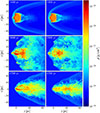 |
Fig. A.1. 2D cuts of the 3D S1 simulation showing rest-mass density in the XY plane at z = 0, with (left panels) and without (right panels) motion of the ejecta. We selected here 3 different moments from the simulation (e.g. A.2 and 3) to show the asymmetries introduced by the orbital motion |

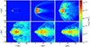 |
Fig. A.2. 2D cuts of the 3D S1 simulation showing rest-mass density in the XY plane at z = 0 with an initially static ejecta. Top left panel: t ≈ 140 yr; top middle panel: t ≈ 1600 yr; top right panel: t ≈ 2400 yr; bottom left panel: t ≈ 3200 yr; bottom middle panel: t ≈ 3700 yr; bottom right panel: t ≈ 4900 yr. |
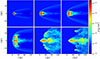 |
Fig. A.3. 2D cuts of the 3D S2 simulation showing rest-mass density in the XY plane at z = 0 with an initially static ejecta. Top left panel: t ≈ 430 yr; top middle panel: t ≈ 1400 yr; top right panel: t ≈ 2300 yr; bottom left panel: t ≈ 2900 yr; bottom middle panel: t ≈ 4000 yr; bottom right panel: t ≈ 4700 yr. |
Appendix B: Simulations table
Simulation parameters; common parameters at the bottom.
All Tables
All Figures
|
Fig. 1. Snapshot of jet-SN interaction during the initial phase to illustrate the setup of the 2D axisymmetric simulations. Upper half: Rest-mass density, ρ. Lower half: Axial velocity, vz. The dashed white line gives the jet-mass fraction contour for the tracer value f = 0.5. The jet flow is filling the grid but in the ejecta region and propagates from left to right. |
| In the text | |
|
Fig. 2. Time evolution of rest-mass density (upper half panels) and axial velocity (lower half panels, mirror of the upper panels) for S1 in 2D. The black lines give the contour of the jet-mass fraction for the tracer value f = 0.5. The jet is propagating from the left to the right. Top left: t ≈ 1600 yr from the start of the simulation; top right: t ≈ 2300 yr; bottom left: t ≈ 3000 yr; bottom right: t ≈ 3800 yr. |
| In the text | |
|
Fig. 3. Time evolution of rest-mass density for S1 in 3D, with six 2D cuts in the XY plane at z = 0. The jet is propagating from the left to the right. Top left: t ≈ 180 yr; top middle: t ≈ 1600 yr; top right: t ≈ 2300 yr; bottom left: t ≈ 3000 yr; bottom middle: t ≈ 3800 yr; bottom right: t ≈ 4700 yr. |
| In the text | |
|
Fig. 4. Time evolution of temperature (upper half panels) and tracer of jet-mass fraction (lower half panels) for S1 in 3D, with 6 2D cuts in the XY plane and at z = 0; the lower half corresponds to the same region shown in the upper half, but inverted with respect to the axis on x = 0. The jet is propagating from the left to the right. Top left: t ≈ 180 yr; top middle: t ≈ 1600 yr; top right: t ≈ 2300 yr; bottom left: t ≈ 3000 yr; bottom middle: t ≈ 3800 yr; bottom right: t ≈ 4700 yr. |
| In the text | |
|
Fig. 5. Coloured surfaces of rest-mass density 3D distribution, in code units, for the evolved structure of simulation S1 at t ≈ 3000 yr, corresponding to the bottom left panel of Fig. 3. The axis of the jet is in the middle of the XZ plane, and the latter propagates along the Y-axis (triad visible in the bottom left of the image) and from left to right; the surfaces show the shocked ejecta interacting with the jet flow, while the nearly transparent red layer surrounding the shocked ejecta outlines the shocked jet region. |
| In the text | |
|
Fig. 6. Same as Fig. 2, but for 2D axisymmetric S2 simulation. Top left: t ≈ 1500 yr; top right: t ≈ 2200 yr; bottom left: t ≈ 2900 yr; bottom right: t ≈ 4000 yr. |
| In the text | |
|
Fig. 7. Same as Fig. 3, but for S2 in 3D. Top left: t ≈ 350 yr; top middle: t ≈ 1500 yr; top right: t ≈ 2200 yr; bottom left: t ≈ 2900 yr; bottom middle: t ≈ 4000 yr; bottom right: t ≈ 4700 yr. |
| In the text | |
|
Fig. 8. Same as Fig. 4, but for S2 in 3D. Top left: t ≈ 350 yr; top middle: t ≈ 1500 yr; top right: t ≈ 2200 yr; bottom left: t ≈ 2900 yr; bottom middle: t ≈ 4000 yr; bottom right: t ≈ 4700 yr. |
| In the text | |
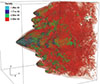 |
Fig. 9. Same as Fig. 5, but for S2 in 3D at t = 4700 yr. |
| In the text | |
|
Fig. 10. Time evolution of jet bow-shock location in S1 (left panel) and S2 (right panel) in 2D and 3D. For the 2D simulations, the calculation is done for three different resolutions: same resolution as the 3D simulation, resolution/2 (i.e. number of cells/2) and resolution ×2 (i.e. number of cells ×2). |
| In the text | |
|
Fig. 11. Specific entropy (normalised to the jet entropy) averaged over domain, [ − 2.5, 2.5] RSN × [ − 2.5, 2.5] RSN of the XZ plane around the jet axis for the 3D simulations; six time steps from S1 (left panel) and S2 (right panel) are shown to accurately follow the dynamical evolution of the ejecta. |
| In the text | |
|
Fig. 12. Time evolution in 3D case of rest-mass density in the lab-frame, D; kinetic ek and internal, u, energy density (normalised to the jet values); and velocity, vy, in vj-units, averaged over the XZ plane at the outflow boundary of the Y-axis for S1 (solid lines) and for S2 (dashed lines). |
| In the text | |
|
Fig. A.1. 2D cuts of the 3D S1 simulation showing rest-mass density in the XY plane at z = 0, with (left panels) and without (right panels) motion of the ejecta. We selected here 3 different moments from the simulation (e.g. A.2 and 3) to show the asymmetries introduced by the orbital motion |
| In the text | |
|
Fig. A.2. 2D cuts of the 3D S1 simulation showing rest-mass density in the XY plane at z = 0 with an initially static ejecta. Top left panel: t ≈ 140 yr; top middle panel: t ≈ 1600 yr; top right panel: t ≈ 2400 yr; bottom left panel: t ≈ 3200 yr; bottom middle panel: t ≈ 3700 yr; bottom right panel: t ≈ 4900 yr. |
| In the text | |
|
Fig. A.3. 2D cuts of the 3D S2 simulation showing rest-mass density in the XY plane at z = 0 with an initially static ejecta. Top left panel: t ≈ 430 yr; top middle panel: t ≈ 1400 yr; top right panel: t ≈ 2300 yr; bottom left panel: t ≈ 2900 yr; bottom middle panel: t ≈ 4000 yr; bottom right panel: t ≈ 4700 yr. |
| In the text | |
Current usage metrics show cumulative count of Article Views (full-text article views including HTML views, PDF and ePub downloads, according to the available data) and Abstracts Views on Vision4Press platform.
Data correspond to usage on the plateform after 2015. The current usage metrics is available 48-96 hours after online publication and is updated daily on week days.
Initial download of the metrics may take a while.