| Issue |
A&A
Volume 704, December 2025
|
|
|---|---|---|
| Article Number | A186 | |
| Number of page(s) | 19 | |
| Section | Stellar atmospheres | |
| DOI | https://doi.org/10.1051/0004-6361/202556118 | |
| Published online | 16 December 2025 | |
H I line observations of 151 evolved stars made with the Nançay Radio Telescope
II. Analysis of the H I and H2 content of AGB star circumstellar envelopes
1
LUX, Observatoire de Paris, Université PSL, Sorbonne Université, CNRS,
5 place Jules Janssen,
92190
Meudon,
France
2
Observatoire Radioastronomique de Nançay, Observatoire de Paris, Université PSL, Université d’Orléans,
18330
Nançay,
France
3
Massachusetts Institute of Technology Haystack Observatory,
99 Millstone Road,
Westford,
MA
01886,
USA
4
LUX, Observatoire de Paris, Université PSL, Sorbonne Université, CNRS,
61 av. de l’Observatoire,
75014
Paris,
France
★ Corresponding author: This email address is being protected from spambots. You need JavaScript enabled to view it.
Received:
26
June
2025
Accepted:
14
October
2025
Abstract
We present an analysis of the results of 21-cm H I line observations of the circumstellar envelopes (CSEs) of a sample of 151 evolved stars, consisting predominantly (85%) of asymptotic giant branch (AGB) stars. This is the first time an analysis could be carried out for the neutral hydrogen constituent of a substantial sample of CSEs of AGB stars. We obtained our observations mainly with the Nançay Radio Telescope (NRT), resulting in 34 clear detections and 21 possible detections. Among the 106 AGB type stars with non-confused H I spectra, 75% are O-rich and 22% are C-rich, while 41% are SRb type semi-regular variables and 38% are Miras. We found no significant biases in the selection or observations of different types of AGB stars. The total H I masses of the detected AGB stars range from 0.002 to 0.1 M⊙, with a mean value of 0.02 M⊙. The mean total H I masses are not significantly different for stars of different types of variability (Miras and semi-regulars). However, there is a difference between O- and C-rich AGB stars, which is due to only three C-rich stars with exceptionally high H I masses (>0.1 M⊙). If we disregard them, there is no significant difference among these types. We compared the total masses of atomic and molecular hydrogen in 34 AGB star CSEs, with the latter estimated from far-infrared imaging of dust, which extends out to about the same radii as the H I. We found that, on average, the H2 masses are ~20 times larger than the H I masses. However, in eight objects, the hydrogen in the CSE is essentially completely atomic. We examined the possible dependence of our results, in particular the H2:H I total mass ratio, on the effective temperature (Teff) of the central star. We find that the H I detection rate of CSEs tends to increase steadily with Teff, but we find no obvious correlation between the H2:H I mass ratio and Teff over the range ~2100–3300 K. Here, we discuss this result in the context of the theoretical prediction that the hydrogen in their CSEs should be mainly atomic for AGB stars warmer than about 2500 K, and mainly molecular for cooler stars. However, the limited fraction in our sample of stars with well-determined temperatures lying below 2500 K prevented us from definitively confirming or refuting the predictions of this model. We discuss a number of effects that might explain the predominantly molecular nature of CSEs, irrespective of stellar temperature. Advancing their interpretation would require further development of mass outflow models for AGB stars of different effective temperatures, as well as comprehensive sets of Teff measurements of this highly time-variable class of stars. We also compared the H I and CO(1–0) line emission of AGB CSEs. The latter emission originates from much smaller radii (<0.01 pc) than the H I (0.75 pc for the resolved sources), and no H2 masses can be determined from it. There is a large spread in the CO:H I integrated line flux ratio (by more than a factor of 100). We found that CO:H I flux ratios generally increase with the H2:H I mass ratio.
Key words: stars: AGB and post-AGB / circumstellar matter / stars: winds, outflows / radio lines: stars
Deceased.
© The Authors 2025
 Open Access article, published by EDP Sciences, under the terms of the Creative Commons Attribution License (https://creativecommons.org/licenses/by/4.0), which permits unrestricted use, distribution, and reproduction in any medium, provided the original work is properly cited.
This article is published in open access under the Subscribe to Open model. This email address is being protected from spambots. You need JavaScript enabled to view it. to support open access publication.
1 Introduction
Asymptotic giant branch (AGB) stars are low-to-intermediate mass stars (~1–8 M⊙) in their final thermonuclear energy production phase (see e.g. the reviews in Habing & Olofsson 2004). They are losing mass through stellar winds, at rates of a few times 10−8 to 10−4 M⊙ yr−1, with the bulk being lost in the form of hydrogen. This leads to the formation of expanding circumstellar envelopes (CSEs), comprised of gas (both atomic and molecular) and dust. Most AGB stars in the Milky Way galaxy have oxygen-rich surface compositions and all of them are variable to some extent (see Sect. 2).
Hydrogen is the most abundant element in AGB mass outflows and while its molecular form (H2) cannot be observed directly, the atomic form (H I) can. Most studies of AGB mass loss have been based on observations of CO spectral lines, providing, in particular, mass-loss rate estimates. Estimates of total masses (i.e. H2 + H I + dust) of CSEs can be made using farinfrared (FIR) continuum observations and assuming gas-to-dust mass ratios (see Sect. 4.2). Other molecules and dust are minor species. The second most abundant element, He, does not show circumstellar lines.
On the other hand, direct observations can be made of the atomic component of hydrogen, using the 21-cm H I line. These provide important information as, for example, the H I in CSEs is much more extended than the CO, the total H I mass can be measured directly without assuming a gas-to-dust ratio, they provide kinematic information on gas flows in CSEs, and the mass fraction of hydrogen that is atomic can be used to test theoretic models of stellar winds.
In a previous paper (Gérard et al. 2024, hereafter Paper I), we presented H I line observations of a sample of 290 evolved stars made mainly with the single-dish 100 m-class Nançay Radio Telescope (NRT), representing over 5000 hours of telescope time. For all 151 objects with non-confused NRT H I spectra, we list the basic properties in Appendix A, for the sake of completeness. In the present paper we seek to better understand our results in the context of the physical properties and evolutionary status of these evolved stars.
Our current analysis is focussed on the 106 AGB stars in our sample (see Sect. 2), which has enabled us to perform a first analysis of the atomic hydrogen constituent of the mass loss in a substantial sample of these evolved stars. This study serves as an important complement to the numerous CO line studies of their molecular gas. We examine the possible dependence of total neutral atomic and molecular hydrogen masses of the CSEs (in particular the H2:H I total mass ratio) on the effective temperature of the central star, using FIR total mass estimates. We also explore whether there are differences in the H I properties between different types of AGB stars in terms of their variability or surface chemical composition.
This paper is organised as follows. In Sect. 2, we discuss the sample, in Sect. 3 the stellar effective temperatures, in Sect. 4 estimates of the molecular hydrogen content of CSEs, and in Sect. 5 we present a comparison of our results to CO line observations. Our results are discussed in Sect. 6 within the framework of a comparison of atomic and molecular hydrogen masses of CSEs. In Sect. 7, we summarise our conclusions.
2 The sample: Variability and surface chemical composition
In Paper I, we presented H I observations of our full sample of 290 evolved stars and indicated the objects whose spectra could not be used for further analysis due to confusion caused by Galactic H I line signals along the line of sight. The remaining sample consists of the 151 objects listed in Table A.1. They are predominantly (85%) AGB stars.
For the analysis presented in this paper, we only used objects with digital NRT spectra. We excluded the 22 objects with less sensitive, non-digital NRT spectra from our initial observations made in 1992/93 (see Paper I; these are flagged as ‘old data’ in Table A.1 and as ‘old’ in Table B.1). We also used Very Large Array (VLA) and Green Bank Telescope (GBT) results (see Table A.1).
The analysis presented here is focussed on the remaining 106 AGB type stars in our sample. Of these, 34 were detected clearly in H I, 18 are possible detections, and for 54 we could estimate upper limits to their total H I masses. In terms of their chemical properties, 75% of these are O-rich and 22% are C-rich, while in terms of variability, the most common types are SRb type semi-regular variables (41%) and long-period regularly variable Miras (38%). More details are given later in this section. Other types are considerably rarer: Lb types, with slowly varying brightness and poorly defined pulsation periods (8%), and SRa and SRc type semi-regulars (5% and 6%, respectively); see e.g. the General Catalogue of Variable Stars (Samus’ et al. 2017) for descriptions of the different types.
In terms of their surface chemical composition, AGB stars are generally divided according to the C/O atom number ratio in their surface matter. The O-rich stars, of spectral type M, have C/O<1, whereas as the C-rich stars, of spectral type C, have C/O > 1, and the intermediary S-type stars have C/O~1. The O-rich stars are predominant in the Milky Way. Among the 106 AGB stars in our sample they represent 74%, while 22% are C-rich and 3% are S-types.
The Mira and SR classes of variables are thought to be linked in terms of evolution, with SR types being the progenitors of Miras (e.g. Kerschbaum & Hron 1992, Szymczak et al. 1995, Whitelock & Feast 2000, and Yeşilyaprak & Aslan 2004). Comparisons of Galactic Miras and SR type stars in terms of some of their basic properties (variability, effective temperatures, ages, initial masses) reveal the following trends (see e.g. Mattei et al. 1997, Feast 2009, Habing & Olofsson 2004, Kerschbaum & Hron 1992, Kerschbaum & Hron 1996, and Kudashkina 2019):
Variability: Miras have quite regular periods of 80 to 1000 days (average ~300 days) and visual amplitudes of ~2 to 9 mag, while SRb type variables show a poorly defined periodicity, superimposed multiple pulsation periods, or alternating periods of regular and irregular variability. When regular, SRb periods are 30 to 1000 days and the amplitudes of the variations in their visible light curves are up to ~2 mag only.
Effective temperatures, Teff: Miras are cooler on average; for our sample the mean Teff for Miras is ~2500 K, and ~2950 K for SRb types (see also Sect. 3).
Ages and initial masses: the bulk of O-rich Miras, with periods of ~300 days, are ~7 Gyr old. They have low initial masses, of order 1.3 M⊙. C-rich Miras have longer periods, on average of 520 days, an average age of 1.8 Gyr and an average initial mass of 1.8 M⊙. O-rich Miras and SRb types have comparable initial masses.
Chemical composition: C-rich stars are much more common among the SR types, as they represent only 5% of our Miras and 32% of the SR types.
3 On effective stellar temperatures of variable AGB stars
One question that arises is whether the effective temperature (Teff) of the central star plays a (key) role in the detectability of H I in its CSE (see also Sect. 6.3). For example, the stellar outflow models of Glassgold & Huggins (1983) predicted that the hydrogen in CSEs should be mainly atomic for Teff higher than about 2500 K, while they would be molecular for cooler stars. However, 2500 K is not a hard limit according to the authors and the model has its limitations, such as ignoring production of H I in CSEs through in situ photodissociation of H2, which we discuss in Sect. 6.
We therefore examined the published Teff values for the stars in our sample. The derivation of stellar effective temperatures is an intricate process, for which various approaches can be used (see e.g. Appendix C of De Beck et al. 2010). It is therefore difficult to estimate uncertainties in Teff values for individual stars, in particular when comparing results derived by different methods, which are usually given without an uncertainty for their particular value. Among the 12 references listed in Table A.1 only four give estimated uncertainties, on average, of ±130 K, which are based on their assessment of the accuracy of the method they applied. Also, De Beck et al. (2010) noted that measured Teff values are more uncertain for Miras, which are colder and more opaque.
However, typically the uncertainties for individual objects and differences in results from different methods are smaller than the large intrinsic variations in effective temperatures that have been reported for the classes of variable stars included in our sample. This is especially relevant in the case of Miras, whose Teff values can vary by as much as ~800 K (see e.g. Pettit & Nicholson 1933; Reid & Goldston 2002). Furthermore, very few publications indicate the phase in the variability cycle of a given star at which the effective temperature was measured, thus limiting the practical applicability of the measurements for testing temperature dependent outflow models. Therefore, it should be emphasised that for any given star the Teff value we list represents but a snapshot measurement during its variability cycle and that its temperature may well pass back and forth across the above-mentioned 2500 K limit as it pulsates.
The statistics that follow are based on the Teff values listed in Table A.1. As mentioned above, some objects have additional published values that differ from these. We found two or more independent measurements of Teff for 17 stars, with an average difference of 380 K. We find no significant difference between the mean Teff values of C- and O-rich stars in our sample, of 2770 K and 2800 K, respectively. This is contrary to the ‘almost complete separation’ between the Teff ranges of the two types of stars noted in Habing & Olofsson (2004), who reproduced a figure from Marigo (2002) which is based on data from Smith & Lambert (1985), Smith & Lambert (1986), and Smith & Lambert (1990) for O-rich stars, and on Bergeat et al. (2001) for C-rich stars. The C-rich stars in the latter four samples are on average about 800 K cooler than the O-rich stars (averages of 2740 K and 3530 K, respectively). In terms of stellar variability, we find that the Miras in our sample are about 500 K cooler on average than the SRb type variables (averages of 2480 K and 2960 K, respectively), in line with for example the findings of van Belle et al. (1997).
4 The total H I and H2 masses of AGB star CSEs
The measurement of total H I masses can be made directly for the gas in the CSEs of AGB stars, since the 21-cm line emission is optically thin. Furthermore, the detectability of the H I line is independent of gas temperature, T, since its absorption coefficient is inversely proportional to T at this low frequency, while its emission coefficient is directly proportional to T (see e.g. Hoai et al. 2015). Observations with a single dish telescope such as the NRT are complicated, however, due to possible confusion due to ubiquitous and often stronger, H I line signals from the surrounding ISM along the line of sight (see Paper I for details of the observing and data reduction procedures). The HPBW of the NRT is always 4′ in the east-west direction, and ≥22′ north-south. For 13 objects, the H I distributions were also mapped with mainly the VLA interferometer at a resolution of about 1′ (see Paper I).
For the strongest sources that were spatially resolved by the NRT beam we could determine integrated ‘total’ H I line profiles using all on-source pointing positions that lie within the extent of the CSE, while for the others we used the ‘peak’ profile measured only within the on-source telescope beam pointed at the star (see Paper I for further details). The measured total H I masses range from 0.002 to 0.1 M⊙, with a mean value of 0.02 M⊙. The mean total H I masses of our sample AGB stars are not significantly different as a function of either their variability class (Miras or semi-regulars), or their chemical composition (O- or C-rich), provided that for the latter comparison we disregarded the three stars with exceptionally high H I masses, >0.1 M⊙ (see Sect. 6.2).
Source diameters were estimated in the East-West direction without correction for the 4′ beam size. For the 25 spatially resolved, clearly detected sources the diameters range from 0.5 to 5 pc, with an average of 1.5 pc, whereas for the 9 unresolved sources, the upper limits range from 0.5 to 1.1 pc, with an average of 0.8 pc.
The H I profiles of our sample stars can be well represented by a Gaussian function. The outflowing, optically thin H I gas is decelerated at the outer edge of the CSE by interaction with the surrounding ISM. The resulting profile shape is a convolution of the effects of expansion, interaction, and thermal broadening, as seen, for example, in the model in Libert et al. (2007). This is in contrast to the shapes of CO line profiles, which for unresolved objects range from rectangular to parabolic, with increasing optical depth (see e.g. Olofsson et al. 1993 and Sect. 5).
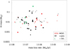 |
Fig. 1 Total H I mass of AGB star CSEs, MHI in M⊙, as a function of mass-loss rate, |
![Mathematical equation: $\[\dot{M}\]$](/articles/aa/full_html/2025/12/aa56118-25/aa56118-25-eq1.png)
4.1 H I mass and mass-loss rates
The total H I mass of the CSEs does not depend on the current mass-loss rate (as derived from CO line observations), as shown in Fig. 1. References to CO line mass-loss rates are listed in Tables in Appendix B of Paper I and the values we used were corrected to the distances adopted in our study. We made clear H I detections of AGB stars with mass-loss rates ranging from 2 × 10⁻⁸ to 2 × 10⁻⁶ M⊙ yr−1 H I (see Sect. 2). However, their mean mass-loss rates do vary as a function of variability class. For the objects listed in Table A.1, we found: 0.13 × 10⁻⁶ M⊙ yr−1 for the Lb types, 1.2 × 10⁻⁶ M⊙ yr−1 for SRb types, and 3.8 × 10⁻⁶ M⊙ yr−1 for Miras.
4.2 H I and H2 mass estimates
One method used to compare total molecular and atomic hydrogen masses of CSEs over similar spatial dimensions is based on FIR observations, which enable estimations of the total mass of their gas (molecular and atomic) + dust constituents. A key assumption is that the dust is uniformly mixed throughout the gas, regardless of whether it is atomic or molecular, so that the thermal FIR emission from dust traces all of the gas. In that case, CSE dust masses derived from their FIR emission can be multiplied by an assumed gas-to-dust mass ratio to estimate the total (gas + dust) mass. The published large gas-to-dust mass ratios (detailed given later in this Section) indicate that the dust mass is a negligible component of the total mass estimated from FIR measurements. Therefore, in practice, a comparison of the ratios of the total FIR (i.e. H I + H2) and H I masses should provide an estimate of the relative contribution of the molecular H2 and atomic H I components.
Maps of the FIR thermal dust emission of CSEs should be a good tracer of their overall gas distribution (atomic + molecular). This is because the small dust grains that emit in the FIR are bound to the gas, as shown by the hydrodynamical models developed by van Marle et al. (2011). An advantage of using FIR images is the weak confusion by surrounding Galactic structures, as compared to the probability of confusion in the H I line.
We focussed on two FIR studies using (1) Herschel satellite images at 70 and 160 μm wavelengths, with a spatial resolution of 6″ at 70 μm (Cox et al. 2012a, and corrigendum in Cox et al. 2012b; herefafter Cox12); and (2) IRAS satellite data at 60 and 100 μm wavelength (Young et al. 1993b and Young et al. 1993a; hereafter Young93), with a ten times coarser resolution of 1′ at 60 μm.
The two sets of images are complementary for our purpose of estimating total H2 + H I hydrogen masses of CSEs since (1) only the higher resolution Herschel images allow a clear separation of the emission from the central source and the CSE, but they have a lower surface brightness sensitivity than the IRAS data, which can lead to an underestimation of the total flux density of the CSE; and (2) IRAS all-sky survey scans were analyzed for a total of 512 evolved stars, selected on a broad range of criteria such as CO line detection, FIR colours, and variability, while the Herschel images were obtained for 78 selected evolved stars, including objects previously resolved by IRAS (Groenewegen et al. 2011), and were aimed at resolving their CSEs.
From the IRAS data, Young93 estimated a ‘point source’ flux density inside the central 1′ diameter beam area and an ‘extended’ flux density outside the central beam diameter. They estimated outer radii of sources by fitting models to all scans of a particular object. From the Herschel data, Cox 12 measured total FIR flux densities within the dust structures visible in the CSEs. They measured the outer radii of dust structures in azimuthally averaged radial FIR emission distributions.
The estimated IRAS 60 μm extended flux densities are on average 1.9 times the measured Herschel 70 μm values, for the 17 objects in our sample with both values available. Compared to the east-west radii of clear NRT H I detections, the 15 IRAS radii are much closer to the H I values, with a mean FIR:H I radius ratio of 0.64 (excluding the outlier RS Cnc), while the Herschel radii are on average 1.9 times smaller than the IRAS values. The outlier in the FIR:H I radius comparison is RS Cnc, with an exceptionally large IRAS FIR:H I radius ratio of about three, but a very small H I radius of 0.17 pc.
The methodology for estimating total gas (H I + H2) + dust masses from FIR images as used by Cox12 is as follows. For the IRAS 60 μm data we used the same model parameters as used by Cox12 for the Herschel 70 μm data. First, the total dust masses were estimated by using the following formula from Li (2005), expressed as
![Mathematical equation: $\[M_{\mathrm{dust}}=0.5 F_\nu \lambda^2 d^2 k^{-1} T_{\mathrm{dust}}^{-1} \kappa_\lambda^{-1}\]$](/articles/aa/full_html/2025/12/aa56118-25/aa56118-25-eq2.png) (1)
(1)
where d is the distance to the star, in cm, Fν is the observed flux density, in erg s−1 cm−2 Hz−1, λ the wavelength, in cm, k the Boltzmann constant in cgs units, Tdust the dust temperature in K, and κλ the dust opacity in cm2 g−1; see Cox et al. (2012a) for further details.
Total gas masses were then derived from the dust masses, assuming values for the gas-to-dust mass ratio. We also corrected the estimated gas + dust masses from Cox et al. (2012b) for the difference in the gas-to-dust mass ratio observed in C- and O-rich stars. This difference was noted, but not corrected for, in Cox12. They assumed a uniform gas-to-dust mass ratio of 200, while noting that the measured ratios are two times higher (400) for C-rich stars and 0.8 times lower (160) for O-rich stars (see e.g. Draine & Lee 1984, Heras & Hony 2005, Li & Draine 2001, and Knapp 1985). We refer to Table 4 for the resulting FIR gas + dust masses estimated using the IRAS 60 μm and Herschel 70 μm and 160 μm data, along with the ratios of FIR 70 μm and H I total masses. The differences in the published gas-to-dust mass ratios indicate that total masses inferred from the FIR emission are uncertain by at least a factor of a few.
We added the Mira IRC+10216 to our analysis, using Herschel 100 μm data from Decin et al. (2011). It was detected in H I with the VLA and the GBT, see Matthews & Reid (2007) and Matthews et al. (2015). We scaled the FIR mass from Decin et al. (2011) to our adopted distance, subtracted the emission originating from the inner 15″ radius, following Cox12, and used our adopted gas-to-dust mass ratio of 400 for C-rich star. This resulted in a total FIR mass of 0.19 M⊙.
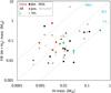 |
Fig. 2 Comparison between FIR total H2 + H I hydrogen masses, MFIR, estimated from FIR data, and total H I masses of AGB star CSEs, both in M⊙. Clear H I detections (det.) are shown as dots, possible detections (pos.) as smaller squares, and upper limits (lim.) as open triangles. Colours indicate different types of variability: red for Miras, black for SR types, and green for L types. FIR masses are based on 60 μm IRAS data or 70 μm Herschel images. The colours of the IRAS data are of a more vivid hue than the Herschel data, such as red vs. orange and black vs. grey. To guide the eye, the three dashed blue lines indicate FIR:H I mass ratios of 100:1, 10:1, and 1:1, respectively. |
4.3 Comparison of H I and H2 masses
In Figure 2, we show the comparison between our total H I masses and the FIR gas + dust masses calculated with the aforementioned difference in dust-to-gas mass ratios between C- and O-rich stars. For each data point, we indicate the status of the H I spectrum (clear detection, possible detection, or upper limit), the variability type of the star (Mira, SR, or Lb), and whether the total gas+dust mass is based on IRAS or Herschel data. To our NRT data we added three H I observations made at the VLA and GBT (a detection of IRC+10216 and upper limits for W Hya and IK Tau) and we used an MFIR for IRC+10216 based on Herschel data from Decin et al. (2011) (see Sect. 4.2).
The total mass of most AGB CSEs appears to be dominated by H2 gas. Evidence to support a molecular state for most of the hydrogen gas in three of the outliers in our sample with the highest H2:H I mass ratios is also indicated by GALEX farUV data on IRC+10216 (Sahai & Chronopoulos 2010; Matthews et al. 2015), o Cet (Martin et al. 2007; Matthews et al. 2008), and U Hya (Sanchez et al. 2015). They all show a detached shell or a cometary tail detected in the far-UV, most likely due to in situ shock-excited H2. We note that such far-UV structures surrounding AGB stars is not an uncommon phenomenon (see e.g. Sahai & Mack-Crane 2014, Ortiz & Guerrero 2023, and Răstău et al. 2023). These results are discussed further in Sect. 6.3.
5 Comparison with CO(1–0) line observations
CO line observations are widely used in studies of AGB stars, as they provide a means to derive the present-day escape velocity and mass-loss rate, as well as the CO photodissociation radius, for example. However, they cannot be used to obtain accurate estimates of the total H2 mass of CSEs. Doing so would require knowledge of such parameters of the duration of the CO outflow and the time dependence of the outflow rate.
We had sufficient data to calculate the CO photodissociation radius, beyond which the CO is expected to be destroyed by the interstellar radiation field, for 19 objects in our AGB sample. For this, we used the photodissociation model of Massarotti et al. (2008) and Olofsson et al. (1993), and adopted CO fractional abundances of fCO = 10−3 for C-rich stars and 2 10−4 for O-rich stars, following Olofsson et al. (2002). We found that the average photodissociation radius of our CSEs in the CO(1–0) line is 2000 AU. This value is about 2.5 times the average radius measured in the CO(2–1) and (3–2) lines for 13 objects in our sample with the Atacama Compact Array by Ramstedt et al. (2020) and Andriantsaralaza et al. (2021).
We expected the radius of the H2 distribution to be considerably larger than that of the CO, as the sizes of H2 (and CO) CSEs are governed by self-shielding (see Morris & Jura 1983), so that due to the high abundance and line strength of H2 its distribution would be much larger. The CSE H2 size depends on the mass-loss rate as ![Mathematical equation: $\[\dot{M}\]$](/articles/aa/full_html/2025/12/aa56118-25/aa56118-25-eq3.png) 0.5, resulting in larger CSEs for objects with higher mass-loss rates (see e.g. Bowers & Knapp 1988 and Matthews et al. 2015). Also, the self-shielding effect is amplified by the deceleration of the stellar wind by the interstellar medium, which will result in accumulation of H2 near the bow shock. The H I gas, on the other hand, is not readily impacted by the interstellar radiation field and may be present over a wide range of distances from the star; the mean radius of our resolved H I CSEs is 0.75 pc, equivalent to 150 000 AU (see Sect. 4.1).
0.5, resulting in larger CSEs for objects with higher mass-loss rates (see e.g. Bowers & Knapp 1988 and Matthews et al. 2015). Also, the self-shielding effect is amplified by the deceleration of the stellar wind by the interstellar medium, which will result in accumulation of H2 near the bow shock. The H I gas, on the other hand, is not readily impacted by the interstellar radiation field and may be present over a wide range of distances from the star; the mean radius of our resolved H I CSEs is 0.75 pc, equivalent to 150 000 AU (see Sect. 4.1).
Thus, when comparing integrated CO and H I line fluxes we have to keep in mind that we are sampling two components in CSEs of not only different composition, molecular or atomic, but also with very different spatial distributions around the star. A further complication is that the CO gas may be optically thick or thin, which cannot always be ascertained with certainty from an analysis of the line profile. We assumed that the entire CO(1–0) line emission from the CSEs in our sample is contained within one beam of a single-dish radio telescope. This assumption is based on our calculated CO photodissociation radii, as well as on interferometric observations made at Plateau de Bure by Neri et al. (1998) and Castro-Carrizo et al. (2010).
Listed in Table B.1 are the individual published integrated CO(1–0) line fluxes, in K km s−1, for the objects in our sample, with literature references and the diameters of the telescopes used, in meters. For unresolved sources (which most are) antenna temperature scales expressed in K are telescope dependent due to differences in beam filling factors. Therefore, in order to be able to compare line fluxes observed with telescopes with diameters ranging from 7 to 30 m, for the calculation of the mean flux, ⟨ICO,corr⟩ in K km s−1, we corrected all published fluxes to a telescope diameter of 20 m. For this, we used the square of the telescope diameter (see e.g. Nyman et al. 1992). On average, this increased the uncorrected published fluxes by a factor of 1.9.
We compared (see Fig. 3) the ICO,corr:FHI integrated line flux ratios to FIR:H I total mass ratios, MFIR:MHI, which are a measure of the H2:H I mass ratios of CSEs (see Sect. 4). We found that objects where the CSE hydrogen is relatively more molecular than atomic in nature tend to have higher CO:H I flux ratios. There is a very large spread in CO: H I integrated line flux ratios, of more than a factor of 100 for H I-detected objects. There is no significant difference between the mean ratios of 19 for Miras and 12 for the SR types. For the clear H I detections, in the four objects where the hydrogen is essentially atomic (MFIR/MHI<3) the average ICO/FHI ratio is 1.6 K/Jy, while for the five where the CSE is molecular (MFIR/MHI>10) the ratio is 140 K/Jy. This shows there will always be molecular CO close to the star, irrespective of the atomic and/or molecular nature of the hydrogen at much larger radii. In addition, combining H I and CO observations helps to improve the development of models of outflows from AGB stars (see e.g. the studies of RS Cnc by Libert et al. 2010b, of RX Lep by Libert et al. 2008, and of V1942 Sgr by Libert et al. 2010a).
The quasi-Gaussian shape of the H I line profiles for our sample (see Sect. 4) is in contrast with the shapes of CO line profiles, which for unresolved objects range from rectangular to parabolic, with increasing optical depth (see e.g. Olofsson et al. 1993). The difference in CO and H I line shape occurs basically because the expansion dominates the CO line profile, emitted relatively close to the star, by a wind that has not yet been slowed down by the surrounding ISM, whereas the H I has been slowed down.
Widths of H I lines are commonly given as FWHM values, while for CO lines expansion velocities are measured, but rarely FWHM values. Expansion velocities are full width at zero power (FWZP) values, which can be readily measured for CO profiles due to their shape, and provide reliable estimates of the gas terminal velocity. They are, however, hard to measure accurately for Gaussian shaped H I profiles. The H I line FWHMs are on average 2.5 times smaller than the CO line expansion velocities (see Table A.1, and Paper I for CO references). We did succeed in determining accurate FWZP widths for a few of the highest signal-to-noise ratio H I profiles measured with the NRT (e.g. Y CVn, see Libert et al. 2007) and VLA (Y UMa, see Matthews et al. 2013), where we could detect the counterpart to the freely expanding wind as observed in CO. For our current sample of non-confused NRT profiles, we estimated FWZP widths based on the velocities where the flux densities first reach the 0 Jy level on both sides of the H I profile peak and found that on average these widths are only 10% smaller than the CO line FWZP values.
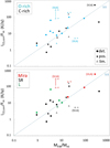 |
Fig. 3 Ratios of CO(1–0) and H I integrated line fluxes, ICO,corr/FHI in K/Jy, as a function of the ratio of FIR (H2 + H I) to H I masses, MFIR/MHI. All published CO fluxes were converted to a telescope diameter of 20 m. Comparisons are shown as a function of chemical composition, C- or O-rich (top panel), and variability: Mira, SR, or L type (lower panel). Clear H I detections (det.) are shown as dots, possible detections (pos.) as smaller squares, and upper limits (lim.) as open triangles. Data points based on H I measurements made with the VLA have been identified. Horizontal arrows indicate points whose MFIR/MHI mass ratios are based on Herschel FIR flux densities, which are systematically lower than IRAS values (see Sect. 4). The colours indicate the various types of objects. Top panel: O-rich (blue), or C-rich (black); lower panel: Mira (red), semi-regular variable (SR, black), and long-period variable (L, green). To guide the eye, a dashed blue line indicates a slope of 1:1 in each panel. |
6 Discussion
In Sect. 6.1 (see below), we examine possible biases that may impact our analysis of the H I-related properties of various kinds of AGB stars. In Sect. 6.2, we then explore possible differences between AGB stars as a function of their chemical composition or type of variability, and in Sect. 6.3 we examine the relation between stellar effective temperature and the atomic and molecular hydrogen content of CSEs.
6.1 Possible biases
In exploring potential biases that may impact the interpretation of results from our H I survey we first examined whether our analysis of the H I-related properties of various kinds of AGB stars could be influenced by: (1) possible biases related to the noise level of the H I spectra; (2) stellar distance; (3) Galactic latitude, and/or local standard of rest (LSR) velocity.
Firstly, with respect to the noise level of H I spectra, we found no significant difference in the root mean square (rms) noise levels of the digital NRT spectra of different types of AGB stars. For example, when examining all available spectra of Miras and SR types, we found mean rms noise levels for the ‘peak’ profiles (see Sect. 4.1) of 0.0057 Jy for Miras and 0.0067 Jy for SR types. For the ‘total’ profiles, which could be determined for the strongest extended detections only, we found 0.025 Jy for Miras and 0.032 Jy for SR types.
Secondly, with respect to distance, for the objects listed in Table A.1 that have Gaia EDR 3 parallaxes, the mean distance of Miras (850 pc) is about twice as large as that of the SR types (390 pc). The Miras have a distance distribution that extends well beyond the ~700 pc limit of the bulk of the semi-regular variables. The mean distance of O-rich AGB stars (560 pc) is similar to that of the C-rich types (600 pc).
Finally, for the Galactic latitude and/or LSR velocity, the NRT single-dish H I observations discussed here are particularly sensitive to the potential presence of ubiquitous ambient Galactic gas clouds within the telescope beam, at both on- and off-source pointing positions. These could cause confusion in the detection of H I that resides within a stellar CSE, especially at low Galactic latitudes or/and at small LSR velocities. We therefore compared various distributions as a function of Galactic latitude and LSR velocity of Miras and SR type variables, and of O-rich and C-rich stars: total number of stars, number of detections, and detection percentages. We found no significant possible biases wherever meaningful statistical comparisons could be made between stars of different types. However, there are not enough clear detections of Lb type variables or C-rich stars for such comparisons.
All in all, we did not find evidence to support any significant biases that could have an impact on our analysis of our H I line data for the various types of AGB stars in our sample related to either H I detection sensitivity, distance, Galactic latitude, and/or LSR velocity.
6.2 Do H I properties depend on stellar chemistry and variability?
We investigated whether there is a significant difference between the H I masses of different types of AGB stars in terms of type of variability (Miras and SR types) as well as surface chemical composition (O- and C-rich). We also checked whether there could be possible selection biases, in terms of distance, for example. For the comparisons, we only used objects with digital NRT spectra and VLA and GBT results (see Table 2).
Listed in Tables 1, 2, and 3 are the following properties for selected AGB stars:
det?: H I detection status – det = clear detection, pos = possible detection;
chem.: chemical composition – C-rich, or O-rich;
var.: variability type;
d: distance, in pc;
Teff: effective temperature, in K;
MHI: total H I mass, in M⊙;
MFIR/MHI: ratio of total FIR:H I masses, based on either IRAS 60 μm or Herschel 70 μm data.
The largest differences between mean values occur for: (1) H I masses of clearly detected C- and O-rich AGB stars (mass ratio of 3.3, and 0.9σ difference, between 0.085 and 0.026 M⊙, respectively); and (2) distances of clearly + possibly H I-detected Miras and SR types (distance ratio of 2.2, with a 3.0σ difference, between 725 and 325 pc, respectively). The H I mass statistics are skewed, however, by three AGB stars with exceptionally large H I masses, MHI > 0.1 M⊙ (see Table 1). All three have Teff>2500 K and are C-rich. Their distances are comparable to those of other H I detected SR and Lb type variables. This concerns two out of the seven C-rich AGB stars among the clear detections, as well as one C-rich star among the possible detections. Compared to other stars with the same chemical composition and H I detection status, these three have 5–28 times higher H I masses. However, the CSEs of these three C-rich stars also have high total H2 masses and, thus, normal H2:H I mass ratios, with FIR:H I mass ratios ranging from 0.9 to 2.7 based on IRAS 60 μm data (see Table 4).
If we disregard the three C-rich stars with very large H I masses, there is no longer any significant difference between C- and O-rich AGB stars. For the clear H I detections, their mean values become 0.020 and 0.012 M⊙, respectively. The Miras and SR types all span the same range (~0.02–0.08 M⊙) in MHI and the average H I masses of the clear detections are indistinguishable, at 0.019 and 0.021 M⊙, respectively. For the clear detections, the detection rates are 22% (8/37) for Miras and 35% (19/54) for the SR types, a factor of 1.6 difference. However, if we consider both clear and possible detections, the percentages become similar, 46% (17/37) for Miras and 50% (27/54) for the SRs. As shown in Sect. 6.1, the Miras have significantly larger distances than the SR types. For the clear detections, the Miras are 1.6 times more distant on average, while for the clear + possible detections they are 2.2 times more distant. As the mean rms noise levels are the same for Miras and SR types (see Sect. 6.1), the differences in distance are largely sufficient to explain the differences in detection rates.
In summary, we did not find a significant difference between the H I masses of different types of AGB stars in terms of either chemistry or variability class. The three stars with exceptionally high H I masses have normal H2:H I mass ratios.
Stars with exceptionally high H I masses.
Stars with the lowest effective temperatures.
6.3 Atomic and molecular hydrogen CSE content as a function of effective temperature
We used the information compiled in the previous steps of the study (described above) to search for a correlation between the mass fraction of hydrogen that is atomic in the CSEs of AGB stars and their stellar effective temperatures. In Figure 4, we plot MFIR/MHI (i.e. the ratio of the total and atomic hydrogen mass of the CSE) versus Teff, where we use the FIR emission as a proxy for the total hydrogen mass (see Sect. 4) and adopt the atomic hydrogen mass derived from 21-cm H I line observations. The two panels show AGB stars of different chemical composition (O- and C-rich) and variability types (Mira, SR, and Lb). Indicated for each data point are the status of the H I spectrum (clear detection, possible detection, or upper limit), whether the FIR data are from IRAS or Herschel, and either the chemical composition (top panel) or variability type (lower panel) of the star. Three VLA H I observations are included in the comparison, a detection of IRC+10216 and upper limits for W Hya and IK Tau, and the MFIR of IRC+10216 is based on Herschel data from Decin et al. (2011).
The vertical red line in Fig. 4 indicates an effective temperature of 2500 K, below which the hydrogen is predicted to be mainly molecular in form according to the mass outflow models of Glassgold & Huggins (1983), although this is rather a soft limit, and not considered to be a ‘tipping point’ by the authors (see more details later in this work). We note that this should be largely independent of the chemical composition of the stellar atmosphere, namely, whether it is O-rich or C-rich. For the clear H I detections the mean FIR:H I mass ratio is 42 based on IRAS data, and 27 and 18 for, respectively, Herschel observations at 70 μm and 160 μm.
Only 4 of the 27 stars have an effective temperature below 2500 K (see Table 2). Two are Miras and two SR types; two are O-rich and two C-rich; two have only lower limits to their FIR:H I mass ratios. If two ratios are listed, these are for IRAS and Herschel data, respectively.
Taken at face value, Figs. 2 and 4 would seem to imply that the H2 mass exceeds the H I mass by a considerable amount in the bulk of the sample. Listed in Table 3 are the objects with the lowest and the highest H2:H I mass ratios, as measured through their MFIR/MHI ratios. For a CSE with a completely atomic content the FIR:H I total mass ratio will be 1.0. There is a significant difference between the presence of variability classes among the objects with lowest and the highest MFIR/MHI ratios: of the eight objects with the lowest ratios, none of them are Miras, six are SR types, and two are Lb. Meanwhile, of the four objects with the highest ratios, two are Miras and two SR types. There is no difference in chemical composition among the two groups, as half of them are O-rich in both categories. No obvious trends are visible in the distribution of FIR:H I mass ratios as a function of Teff, when examined as a function of variability type. Neither did we find a trend depending on the chemical composition of the star, O-rich or C-rich.
Although the detected H I masses do not increase with Teff, the rate of H I detections does increase steadily with Teff (see Fig. 5, from on average 23% below 2500 K to 50% above 3000 K, for the clear detections only, and up to 67% if we include the possible detections. The statistical uncertainty in the detection rates is ±27%, for a confidence level of 95%. This means that the 50% difference in detection rate between the lowest and highest temperature bins for clear + possible detections is at about two times the uncertainty level. This may indicate an overall increase in H I mass for warmer stars. On the other hand, it is difficult to ascertain if the mean H2 mass changes significantly with temperature, due to the large scatter in MFIR as a function of Teff. All in all, this analysis does not appear to provide additional information on the H2:H I mass ratio as a function of Teff.
Several additional factors may also complicate the interpretation of the NRT H I data as a function of Teff in the context of the Glassgold & Huggins (1983) atmospheric outflow model. We discuss these in turn.
Firstly, ann effective temperature of 2500 K was not presented by the authors as a ‘tipping point’ for the H I or H2 nature of CSEs. They stated that for stars hotter than 3000 K, the hydrogen entering the circumstellar envelope is most likely atomic, while for stars cooler than 2000 K, it is mainly molecular and will remain so out to large radii. They also noted that the H2:H I ratio is sensitive to the mass outflow rate, which is three times higher in Miras than in SRb types for our sample, and 30 times that of Lb types (see Sect. 2).
Secondly, the model does not account for the contribution to the total H I mass resulting from H2 photodissociated in situ within the CSE; this process does not depend on the Teff of the central star. Although the authors had examined the effects of photodissociation in a previous paper (Huggins & Glassgold 1982) and discussed its implications for the case of IRC+10216 in Glassgold & Huggins (1983), they did not include it in the model calculations we refer to here.
In their analysis of imaging observations of the eponymous Mira variable o Ceti in both CO and H I, where they discuss the crucial effects of self-shielding against UV radiation from the ISM (see Sect. 5), Bowers & Knapp (1988) considered that onethird of the hydrogen leaving the star is in atomic form, and that the rest of the H I in its CSE would result from photodissociation. They also mention the possibility that at least part of, if not all, the hydrogen would leave the star in atomic form only during the maximum, hottest phase of the pulsation.
Thirdly, there may be a systematic bias in the Teff measurements for certain Mira variables. As noted by Olofsson et al. (1993), the higher column density of cold Mira CSEs makes it difficult to measure the true effective temperatures of the central stars, and published values could be overestimated.
Finally, there may be possible changes in mass-loss rates of AGB stars over time. In our analysis we have considered the current Teff, mass-loss rate and variability type of the central star. However, some (or all) of these properties may well have been different throughout the ~100 000 year-long mass-loss history that lead to the formation of the CSEs as traced by H I (see e.g. Habing & Olofsson 2004).
In summary, based on our analysis of the available data on global H I and H2 masses of AGB CSEs, we can neither definitively confirm nor refute the dependence of the H2:H I total mass ratio of CSEs on the stellar effective temperature indicated by the outflow model of Glassgold & Huggins (1983). This is due to the small fraction of stars cooler than 2500 K in our sample.
Stars with the lowest and highest H2:H I mass ratios.
Total H I and FIR (H I + H2 + dust) masses of CSEs.
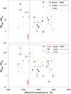 |
Fig. 4 Comparison of the mass fraction of hydrogen that is atomic in the CSEs of AGB stars as a function of stellar effective temperature. The y-axis shows MFIR/MHI, the ratio of the total (molecular plus atomic) hydrogen mass of the CSE (as estimated from FIR measurements; see Sect. 4) to the H I mass of the CSE as measured from H I 21 cm line observations. The x-axis shows Teff, in K. Comparisons are shown as a function of chemical composition of the star (C- or O rich; top panel), and variability class (Mira, SR or L type; lower panel). Clear H I detections (det.) are shown as dots, possible detections (pos.) as smaller squares, and upper limits (lim.) as open triangles. Colours indicate different types of variability: red for Miras, black for SR types, and green for L types. FIR masses are based on 60 μm IRAS data or 70 μm Herschel images. In both panels, the colours of the points where the total hydrogen masses were derived from IRAS data are of a more vivid hue than of the Herschel data, such as red vs. orange and black vs. grey. The red vertical dashed line indicates the 2500 K soft limit around which the H2:H I mass ratio is theoretically predicted to change (see text). |
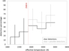 |
Fig. 5 Distributions of H I detection rates as a function of effective temperature of the central star, for clear detections (black line) and for clear + possible detections (grey line), in bins of 300 K width in Teff. The vertical lines indicate statistical uncertainties for a confidence level of 95%. |
7 Conclusions
We present the first-ever analysis of the results of 21-cm H I line observations of the CSEs of a substantial sample of 106 AGB stars. The relatively large beam size of the NRT, used for the bulk of the measurements analyzed here, enabled the derivation of total H I masses and source sizes, though not of the detailed distributions of H I within the CSEs.
The total H I masses range from 0.002 to 0.1 M⊙, with a mean value of 0.02 M⊙. We found no significant differences depending on either stellar surface chemical composition (O-rich versus C-rich) or variability class (Mira, SR, or Lb).
We computed estimates of the total atomic and molecular hydrogen masses of the CSEs using published FIR imaging observations and compared these to measurements of the H I masses derived from 21 cm line observations. We found that in the bulk of the CSEs the hydrogen is predominantly in a molecular state, with an average H2:H I total mass ratio of order 20. In some of the objects with the highest H2:H I mass ratios, the molecular state of the hydrogen can be corroborated by published GALEX far-UV detections that are thought to result from locally shocked H2. In about one-third of the CSEs, however, the hydrogen is essentially entirely atomic.
There is no evidence of a significant difference in chemical composition (O- versus C-rich) for stars with the most extreme H2:H I mass ratios, but there is a difference in variability class: those with the lowest ratios are predominantly semi-regular variables (75%) and none of them are Miras, whereas those with the highest ratios are Miras and semi-regulars in about equal measure.
The theoretical outflow model of Glassgold & Huggins (1983) predicts that the CSEs of AGB stars should be mainly atomic for an effective stellar temperature larger than about 2500 K, and molecular for cooler stars. While the CSEs with the highest H I masses in our sample occur around stars with Teff > 2500 K, we find, however, that the CSEs of some stars warmer than 2500 K appear to have significant molecular hydrogen fractions. Furthermore, there is no evidence of a systematic change in the H2:H I mass ratio at Teff ~ 2500 K. One limitation in our analysis, however, is that only four of the 27 H I-detected stars have an effective temperature below 2500 K.
Furthermore, any analysis of the relation between the H2:H I mass ratio and stellar effective temperature is complicated by the uncertain contribution of H I formed in situ within the CSE from UV-photodissociated H2. This is in addition to H I that has flowed out as such from the star into the CSE. We note that this in situ effect does not depend on the effective temperature of the star.
In summary, the small fraction of stars with Teff < 2500 K prevented us from definitively confirming or refuting the dependence of the molecular hydrogen fraction of a CSE on the stellar effective temperature predicted by the outflow model of Glassgold & Huggins (1983). However, to better analyze the effect of the stellar effective temperature on the atomic and molecular hydrogen content of CSEs of AGB stars, more comprehensive sets of measurements are needed of the highly time-variable effective temperature for individual stars, as well as improved sets of stellar mass-loss models for stars across a range of different temperatures. Finally, following up on one of the goals of our study as mentioned in Paper I, our results indicate a number of suitable candidates for follow-up imaging and mapping studies in the 21-cm H I line to be carried out at a (much) higher spatial resolution.
Acknowledgements
This paper is dedicated to the memory of Nguyên Quang Riêu, who initiated this research. We wish to thank the staff of the Nançay Radio Telescope for their support with the observations over the past 30 years. We also want to thank the anonymous referee for their very useful comments. The Nancay Radio Observatory is operated by the Paris Observatory, associated with the French Centre National de la Recherche Scientifique. This research has made use of the SIMBAD database, operated at CDS, Strasbourg, France. LDM was supported by grant AST-2107681 from the National Science Foundation.
References
- Andriantsaralaza, M., Ramstedt, S., Vlemmings, W. H. T., et al. 2021, A&A, 653, A53 [NASA ADS] [CrossRef] [EDP Sciences] [Google Scholar]
- Bergeat, J., Knapik, A., & Rutily, B. 2001, A&A, 369, 178 [NASA ADS] [CrossRef] [EDP Sciences] [Google Scholar]
- Bowers, P. F., & Knapp, G. R. 1988, ApJ, 332, 299 [NASA ADS] [CrossRef] [Google Scholar]
- Brelstaff, T., Lloyd, C., Markham, T., & McAdam, D. 1997, J. Br. Astron. Assoc., 107, 135 [Google Scholar]
- Bujarrabal, V., Planesas, P., Gomez-Gonzalez, J., Martin-Pintado, J., & del Romero, A. 1986, A&A, 162, 157 [Google Scholar]
- Castro-Carrizo, A., Quintana-Lacaci, G., Neri, R., et al. 2010, A&A, 523, A59 [NASA ADS] [CrossRef] [EDP Sciences] [Google Scholar]
- Cox, N. L. J., Kerschbaum, F., van Marle, A. J., et al. 2012a, A&A, 537, A35 [NASA ADS] [CrossRef] [EDP Sciences] [Google Scholar]
- Cox, N. L. J., Kerschbaum, F., van Marle, A. J., et al. 2012b, A&A, 543, C1 [NASA ADS] [CrossRef] [EDP Sciences] [Google Scholar]
- Danilovich, T., Teyssier, D., Justtanont, K., et al. 2015, A&A, 581, A60 [NASA ADS] [CrossRef] [EDP Sciences] [Google Scholar]
- De Beck, E., Decin, L., de Koter, A., et al. 2010, A&A, 523, A18 [NASA ADS] [CrossRef] [EDP Sciences] [Google Scholar]
- Decin, L., Cherchneff, I., Hony, S., et al. 2008, A&A, 480, 431 [NASA ADS] [CrossRef] [EDP Sciences] [Google Scholar]
- Decin, L., Royer, P., Cox, N. L. J., et al. 2011, A&A, 534, A1 [NASA ADS] [CrossRef] [EDP Sciences] [Google Scholar]
- Díaz-Luis, J. J., Alcolea, J., Bujarrabal, V., et al. 2019, A&A, 629, A94 [NASA ADS] [CrossRef] [EDP Sciences] [Google Scholar]
- Draine, B. T., & Lee, H. M. 1984, ApJ, 285, 89 [NASA ADS] [CrossRef] [Google Scholar]
- Dumm, T., & Schild, H. 1998, New A, 3, 137 [CrossRef] [Google Scholar]
- Dyck, H. M., van Belle, G. T., & Thompson, R. R. 1998, AJ, 116, 981 [NASA ADS] [CrossRef] [Google Scholar]
- Feast, M. W. 2009, in AGB Stars and Related Phenomena, eds. T. Ueta, N. Matsunaga, & Y. Ita, 48 [Google Scholar]
- Gaia Collaboration 2020, VizieR Online Data Catalog, I/350 (Gaia EDR 3) [Google Scholar]
- Gardan, E., Gérard, E., & Le Bertre, T. 2006, MNRAS, 365, 245 [NASA ADS] [CrossRef] [Google Scholar]
- Gérard, E., & Le Bertre, T. 2003, A&A, 397, L17 [NASA ADS] [CrossRef] [EDP Sciences] [Google Scholar]
- Gérard, E., & Le Bertre, T. 2006, AJ, 132, 2566 [CrossRef] [Google Scholar]
- Gérard, E., van Driel, W., Matthews, L. D., et al. 2024, A&A, 692, A54 [NASA ADS] [CrossRef] [EDP Sciences] [Google Scholar]
- Glassgold, A. E., & Huggins, P. J. 1983, MNRAS, 203, 517 [NASA ADS] [Google Scholar]
- Groenewegen, M. A. T., Baas, F., Blommaert, J. A. D. L., et al. 1999, A&AS, 140, 197 [NASA ADS] [CrossRef] [EDP Sciences] [Google Scholar]
- Groenewegen, M. A. T., Waelkens, C., Barlow, M. J., et al. 2011, A&A, 526, A162 [NASA ADS] [CrossRef] [EDP Sciences] [Google Scholar]
- Habing, H. J., & Olofsson, H. 2004, Asymptotic Giant Branch Stars (Astronomy and Astrophysics Library, Springer-Verlag) [Google Scholar]
- Hawkins, G., & Proctor, D. 1993, in European Southern Observatory Conference and Workshop Proceedings, 46, 461 [NASA ADS] [Google Scholar]
- Heras, A. M., & Hony, S. 2005, A&A, 439, 171 [NASA ADS] [CrossRef] [EDP Sciences] [Google Scholar]
- Hoai, D. T., Matthews, L. D., Winters, J. M., et al. 2014, A&A, 565, A54 [NASA ADS] [CrossRef] [EDP Sciences] [Google Scholar]
- Hoai, D. T., Nhung, P. T., Gérard, E., et al. 2015, MNRAS, 449, 2386 [Google Scholar]
- Hoai, D. T., Nhung, P. T., Matthews, L. D., Gérard, E., & Le Bertre, T. 2017, Res. Astron. Astrophys., 17, 067 [CrossRef] [Google Scholar]
- Huggins, P. J., & Glassgold, A. E. 1982, ApJ, 252, 201 [NASA ADS] [CrossRef] [Google Scholar]
- Kerschbaum, F., & Hron, J. 1992, A&A, 263, 97 [NASA ADS] [Google Scholar]
- Kerschbaum, F., & Hron, J. 1996, A&A, 308, 489 [NASA ADS] [Google Scholar]
- Kerschbaum, F., & Olofsson, H. 1998, A&A, 336, 654 [NASA ADS] [Google Scholar]
- Kerschbaum, F., & Olofsson, H. 1999, A&AS, 138, 299 [NASA ADS] [CrossRef] [EDP Sciences] [Google Scholar]
- Kiss, L. L., Szabó, G. M., & Bedding, T. R. 2006, MNRAS, 372, 1721 [Google Scholar]
- Knapp, G. R. 1985, ApJ, 293, 273 [NASA ADS] [CrossRef] [Google Scholar]
- Knapp, G. R. 1986, ApJ, 311, 731 [NASA ADS] [CrossRef] [Google Scholar]
- Knapp, G. R., & Morris, M. 1985, ApJ, 292, 640 [NASA ADS] [CrossRef] [Google Scholar]
- Knapp, G. R., Young, K., Lee, E., & Jorissen, A. 1998, ApJS, 117, 209 [CrossRef] [Google Scholar]
- Kudashkina, L. S. 2019, Astrophysics, 62, 556 [NASA ADS] [CrossRef] [Google Scholar]
- Le Bertre, T., & Gérard, E. 2004, A&A, 419, 549 [NASA ADS] [CrossRef] [EDP Sciences] [Google Scholar]
- Levesque, E. M., Massey, P., Olsen, K. A. G., et al. 2005, ApJ, 628, 973 [Google Scholar]
- Li, A. 2005, in American Institute of Physics Conference Series, 761, 123 [Google Scholar]
- Li, A., & Draine, B. T. 2001, ApJ, 554, 778 [Google Scholar]
- Libert, Y., Gérard, E., & Le Bertre, T. 2007, MNRAS, 380, 1161 [Google Scholar]
- Libert, Y., Le Bertre, T., Gérard, E., & Winters, J. M. 2008, A&A, 491, 789 [NASA ADS] [CrossRef] [EDP Sciences] [Google Scholar]
- Libert, Y., Gérard, E., Thum, C., et al. 2010a, A&A, 510, A14 [NASA ADS] [CrossRef] [EDP Sciences] [Google Scholar]
- Libert, Y., Winters, J. M., Le Bertre, T., Gérard, E., & Matthews, L. D. 2010b, A&A, 515, A112 [NASA ADS] [CrossRef] [EDP Sciences] [Google Scholar]
- Lindqvist, M., Nyman, L. A., Olofsson, H., & Winnberg, A. 1988, A&A, 205, L15 [Google Scholar]
- Margulis, M., van Blerkom, D. J., Snell, R. L., & Kleinmann, S. G. 1990, ApJ, 361, 673 [NASA ADS] [CrossRef] [Google Scholar]
- Marigo, P. 2002, A&A, 387, 507 [NASA ADS] [CrossRef] [EDP Sciences] [Google Scholar]
- Marigo, P., Girardi, L., Bressan, A., et al. 2008, A&A, 482, 883 [NASA ADS] [CrossRef] [EDP Sciences] [Google Scholar]
- Martin, D. C., Seibert, M., Neill, J. D., et al. 2007, Nature, 448, 780 [NASA ADS] [CrossRef] [Google Scholar]
- Massarotti, A., Latham, D. W., Stefanik, R. P., & Fogel, J. 2008, AJ, 135, 209 [Google Scholar]
- Mattei, J. A., Foster, G., Hurwitz, L. A., et al. 1997, in ESA Special Publication, 402, 269 [Google Scholar]
- Matthews, L. D., & Reid, M. J. 2007, AJ, 133, 2291 [NASA ADS] [CrossRef] [Google Scholar]
- Matthews, L. D., Libert, Y., Gérard, E., Le Bertre, T., & Reid, M. J. 2008, ApJ, 684, 603 [CrossRef] [Google Scholar]
- Matthews, L. D., Libert, Y., Gérard, E., et al. 2011, AJ, 141, 60 [NASA ADS] [CrossRef] [Google Scholar]
- Matthews, L. D., Le Bertre, T., Gérard, E., & Johnson, M. C. 2013, AJ, 145, 97 [CrossRef] [Google Scholar]
- Matthews, L. D., Gérard, E., & Le Bertre, T. 2015, MNRAS, 449, 220 [NASA ADS] [CrossRef] [Google Scholar]
- McDonald, I., Zijlstra, A. A., & Boyer, M. L. 2012, MNRAS, 427, 343 [Google Scholar]
- Menten, K. M., Reid, M. J., Kamiński, T., & Claussen, M. J. 2012, A&A, 543, A73 [NASA ADS] [CrossRef] [EDP Sciences] [Google Scholar]
- Morris, M., & Jura, M. 1983, ApJ, 264, 546 [Google Scholar]
- Neri, R., Kahane, C., Lucas, R., Bujarrabal, V., & Loup, C. 1998, A&AS, 130, 1 [NASA ADS] [CrossRef] [EDP Sciences] [Google Scholar]
- Nyman, L. A., Booth, R. S., Carlstrom, U., et al. 1992, A&AS, 93, 121 [NASA ADS] [Google Scholar]
- Ohnaka, K., Weigelt, G., & Hofmann, K. H. 2016, A&A, 589, A91 [NASA ADS] [CrossRef] [EDP Sciences] [Google Scholar]
- Olofsson, H., Eriksson, K., & Gustafsson, B. 1987, A&A, 183, L13 [NASA ADS] [Google Scholar]
- Olofsson, H., Eriksson, K., & Gustafsson, B. 1988, A&A, 196, L1 [NASA ADS] [Google Scholar]
- Olofsson, H., Eriksson, K., Gustafsson, B., & Carlstrom, U. 1993, ApJS, 87, 267 [NASA ADS] [CrossRef] [Google Scholar]
- Olofsson, H., González Delgado, D., Kerschbaum, F., & Schöier, F. L. 2002, A&A, 391, 1053 [NASA ADS] [CrossRef] [EDP Sciences] [Google Scholar]
- Ortiz, R., & Guerrero, M. A. 2023, MNRAS, 522, 811 [NASA ADS] [CrossRef] [Google Scholar]
- Pettit, E., & Nicholson, S. B. 1933, PASP, 45, 194 [Google Scholar]
- Ramstedt, S., Schöier, F. L., & Olofsson, H. 2009, A&A, 499, 515 [NASA ADS] [CrossRef] [EDP Sciences] [Google Scholar]
- Ramstedt, S., Vlemmings, W. H. T., Doan, L., et al. 2020, A&A, 640, A133 [EDP Sciences] [Google Scholar]
- Reid, M. J., & Goldston, J. E. 2002, ApJ, 568, 931 [NASA ADS] [CrossRef] [Google Scholar]
- Rodríguez, L. F., Goss, W. M., & Williams, R. 2002, ApJ, 574, 179 [CrossRef] [Google Scholar]
- Răstău, V., Mečina, M., Kerschbaum, F., et al. 2023, A&A, 680, A12 [NASA ADS] [CrossRef] [EDP Sciences] [Google Scholar]
- Sahai, R., & Chronopoulos, C. K. 2010, ApJ, 711, L53 [NASA ADS] [CrossRef] [Google Scholar]
- Sahai, R., & Mack-Crane, G. P. 2014, AJ, 148, 74 [NASA ADS] [CrossRef] [Google Scholar]
- Samus’, N. N., Kazarovets, E. V., Durlevich, O. V., Kireeva, N. N., & Pastukhova, E. N. 2017, Astron. Rep., 61, 80 [Google Scholar]
- Sanchez, E., Montez, Jr., R., Ramstedt, S., & Stassun, K. G. 2015, ApJ, 798, L39 [Google Scholar]
- Smith, V. V., & Lambert, D. L. 1985, ApJ, 294, 326 [NASA ADS] [CrossRef] [Google Scholar]
- Smith, V. V., & Lambert, D. L. 1986, ApJ, 311, 843 [Google Scholar]
- Smith, V. V., & Lambert, D. L. 1990, ApJS, 72, 387 [NASA ADS] [CrossRef] [Google Scholar]
- Szymczak, M., Le Squeren, A. M., Sivagnanam, P., Tran Minh, F., & Fournier, A. 1995, A&A, 297, 494 [Google Scholar]
- Thirumalai, A., & Heyl, J. S. 2013, MNRAS, 430, 1359 [NASA ADS] [CrossRef] [Google Scholar]
- van Belle, G. T., Dyck, H. M., Benson, J. A., & Lacasse, M. G. 1996, AJ, 112, 2147 [NASA ADS] [CrossRef] [Google Scholar]
- van Belle, G. T., Dyck, H. M., Thompson, R. R., Benson, J. A., & Kannappan, S. J. 1997, AJ, 114, 2150 [Google Scholar]
- van Belle, G. T., Thompson, R. R., & Creech-Eakman, M. J. 2002, AJ, 124, 1706 [NASA ADS] [CrossRef] [Google Scholar]
- van Marle, A. J., Meliani, Z., Keppens, R., & Decin, L. 2011, ApJ, 734, L26 [NASA ADS] [CrossRef] [Google Scholar]
- Whitelock, P., & Feast, M. 2000, MNRAS, 319, 759 [Google Scholar]
- Yeşilyaprak, C., & Aslan, Z. 2004, MNRAS, 355, 601 [CrossRef] [Google Scholar]
- Young, K. 1995, ApJ, 445, 872 [NASA ADS] [CrossRef] [Google Scholar]
- Young, K., Phillips, T. G., & Knapp, G. R. 1993a, ApJ, 409, 725 [CrossRef] [Google Scholar]
- Young, K., Phillips, T. G., & Knapp, G. R. 1993b, ApJS, 86, 517 [NASA ADS] [CrossRef] [Google Scholar]
- Zuckerman, B., & Dyck, H. M. 1986, ApJ, 304, 394 [CrossRef] [Google Scholar]
- Zuckerman, B., & Dyck, H. M. 1989, A&A, 209, 119 [NASA ADS] [Google Scholar]
A description of GCVS types is given in https://cdsarc.cds.unistra.fr/ftp/cats/B/gcvs/vartype.txt
Appendix A Summary of results of the NRT H I observations
In Table A.1, we list the following elements for the 149 objects in our sample which have either clear NRT H I detections (34 objects, top part of the table), possible H I detections (21 objects, middle part), or upper limits to their H I lines (94 objects, lower part). In addition, two objects are listed whose NRT spectra were confused but which were observed with the VLA: IRC +10216 and W Aql (see hereafter). For literature reference to values that do not have a reference listed here, we refer to Paper I.
Name: common catalogue name of the target. An ‘n’ after a name indicates that it is clearly not an AGB star, a ‘d’ that we consider its classification as an AGB to be dubious;
var.: target type. Primarily the variability type as listed in Version 5.1 of the General Catalogue of Variable Stars, GCVS (Samus’ et al. 2017)1. If an object is not included in the GCVS, other identifiers are listed in brackets: (HPM) = high proper motion star, (PN) = planetary nebula, and (pPN) = proto-PN. For the supergiant μ Cep we adopted the SRc variability class from Kiss et al. (2006) instead of the δ Cep class listed in the GCVS;
per.: variability period as listed in the GCVS, in days. For the supergiant μ Cep the GCVS lists a variability period 3.8 days, which appears to be erroneous. We instead adopted the period of 700: days that was indicated by Brelstaff et al. (1997);
Spec.: spectral type of the star, as retrieved from the SIMBAD database;
Teff & ref.: effective temperature of the star, in K, and its literature reference;
d: distance of the target, based mainly on its parallax from the Gaia EDR 3, Gaia Collaboration 2020), in pc. Values in brackets are from other sources, see the Appendix in Paper I;
V lit.: published radial velocity of the target in the Local Standard of Rest (LSR) reference frame, in km s−1;
Vexp: literature expansion velocity measured from CO or OH 1612 MHz line observations, in km s−1. If a pair of values was published for a two-velocity component CO line fit, the largest value is listed here;
![Mathematical equation: $\[\dot{M}\]$](/articles/aa/full_html/2025/12/aa56118-25/aa56118-25-eq6.png) & ref.: literature mass-loss rates, in M⊙ yr−1, and its literature reference;
& ref.: literature mass-loss rates, in M⊙ yr−1, and its literature reference;FWHM: our full width half maximum of the Gaussian fitted to the NRT H I line profile, in km s−1;
MHI: our total H I mass, in M⊙;
diam.: our estimated angular diameter of the H I CSE in the East-West direction, in parsec;
-
H I notes: references to previously published H I studies, and an ‘old data’ flag to denote the less sensitive, non-digital NRT H I spectra obtained during our initial observing campaign in 1992/1993 (see Sect. 2).
Details on the two listed objects with confused NRT spectra observed with the VLA:
IRC + 10216: VLA detection by Matthews et al. (2015). We adopted their distance of 130 pc from Menten et al. (2012) and total H I mass of 0.0032 M⊙. The listed Vexp and
![Mathematical equation: $\[\dot{M}\]$](/articles/aa/full_html/2025/12/aa56118-25/aa56118-25-eq7.png) values are based on CO line data from Knapp et al. (1998);
values are based on CO line data from Knapp et al. (1998);W Hya: VLA non-detection by Hawkins & Proctor (1993). The listed Vexp and
![Mathematical equation: $\[\dot{M}\]$](/articles/aa/full_html/2025/12/aa56118-25/aa56118-25-eq8.png) values are based on CO line data from Young (1995).
values are based on CO line data from Young (1995).
For non-detections, conservative upper limits to their H I masses were estimated for a flux density level of three times the rms noise level in their spectra and a line width of two times the CO line expansion velocity (which on average is 3.4 times larger than the H I line FWHM); in case no CO line observations were available we used a width of 20 km s−1, that is twice the average line width of the CO detections. For objects flagged as ‘old data’ (see Sect. 2) we used the upper limit to the H I line flux density, Speak, as given in Paper I; these estimates made by eye correspond to about the 3σ level. A number of the references to H I studies listed in the Tables concern H I imaging and mapping observations made with the Very Large Array (VLA) and the Green Bank Telescope, see Paper I for details.
Basic data of the evolved stars and their CSEs
Appendix B Integrated CO(1-0) line fluxes
In Table B.1, we list the results of our literature search for CO(1-0) line detections of objects in our sample. The objects whose names have been flagged as ‘old’ are those for which only less sensitive, non-digital H I spectra are available from our 1992/1993 observing campaign (see Sect. 2). We found published CO line observations for 55 (= 56%) of our total sample of 96 objects with non-confused H I spectra: 18 (53%) for the 34 clear H I detections, 8 (38%) for the 21 possible H I detections, and 28 (68%) for the 41 H I upper limits.
The following elements are listed in the table. For further details on variability type and spectral classification we refer to Table A.1.
Name: common catalogue name of the target;
var.: variability type of the star;
Spec.: spectral type of the star;
<ICO,corr>: average integrated CO(1-0) line fluxes, in K km s−1. These are based on the individual published fluxes, ICO, after correcting them to a telescope diameter of 20 m, using the square of the telescope diameter. This was done in order to be able to compare line fluxes of unresolved sources made with telescopes with quite different sizes (see Sect. 5);
ICO: individual published integrated CO(1-0) line fluxes, in K km s−1, together with the size of the telescope used, in meters, and literature references;
FHI: integrated H I line fluxes, in Jy km s−1, based on the total H I masses and distances listed in Table A.1;
ICO,corr/FHI: ratio of the integrated CO(1-0) and H I line fluxes.
Published integrated CO(1-0) line fluxes
All Tables
All Figures
|
Fig. 1 Total H I mass of AGB star CSEs, MHI in M⊙, as a function of mass-loss rate, |
| In the text | |
|
Fig. 2 Comparison between FIR total H2 + H I hydrogen masses, MFIR, estimated from FIR data, and total H I masses of AGB star CSEs, both in M⊙. Clear H I detections (det.) are shown as dots, possible detections (pos.) as smaller squares, and upper limits (lim.) as open triangles. Colours indicate different types of variability: red for Miras, black for SR types, and green for L types. FIR masses are based on 60 μm IRAS data or 70 μm Herschel images. The colours of the IRAS data are of a more vivid hue than the Herschel data, such as red vs. orange and black vs. grey. To guide the eye, the three dashed blue lines indicate FIR:H I mass ratios of 100:1, 10:1, and 1:1, respectively. |
| In the text | |
|
Fig. 3 Ratios of CO(1–0) and H I integrated line fluxes, ICO,corr/FHI in K/Jy, as a function of the ratio of FIR (H2 + H I) to H I masses, MFIR/MHI. All published CO fluxes were converted to a telescope diameter of 20 m. Comparisons are shown as a function of chemical composition, C- or O-rich (top panel), and variability: Mira, SR, or L type (lower panel). Clear H I detections (det.) are shown as dots, possible detections (pos.) as smaller squares, and upper limits (lim.) as open triangles. Data points based on H I measurements made with the VLA have been identified. Horizontal arrows indicate points whose MFIR/MHI mass ratios are based on Herschel FIR flux densities, which are systematically lower than IRAS values (see Sect. 4). The colours indicate the various types of objects. Top panel: O-rich (blue), or C-rich (black); lower panel: Mira (red), semi-regular variable (SR, black), and long-period variable (L, green). To guide the eye, a dashed blue line indicates a slope of 1:1 in each panel. |
| In the text | |
|
Fig. 4 Comparison of the mass fraction of hydrogen that is atomic in the CSEs of AGB stars as a function of stellar effective temperature. The y-axis shows MFIR/MHI, the ratio of the total (molecular plus atomic) hydrogen mass of the CSE (as estimated from FIR measurements; see Sect. 4) to the H I mass of the CSE as measured from H I 21 cm line observations. The x-axis shows Teff, in K. Comparisons are shown as a function of chemical composition of the star (C- or O rich; top panel), and variability class (Mira, SR or L type; lower panel). Clear H I detections (det.) are shown as dots, possible detections (pos.) as smaller squares, and upper limits (lim.) as open triangles. Colours indicate different types of variability: red for Miras, black for SR types, and green for L types. FIR masses are based on 60 μm IRAS data or 70 μm Herschel images. In both panels, the colours of the points where the total hydrogen masses were derived from IRAS data are of a more vivid hue than of the Herschel data, such as red vs. orange and black vs. grey. The red vertical dashed line indicates the 2500 K soft limit around which the H2:H I mass ratio is theoretically predicted to change (see text). |
| In the text | |
|
Fig. 5 Distributions of H I detection rates as a function of effective temperature of the central star, for clear detections (black line) and for clear + possible detections (grey line), in bins of 300 K width in Teff. The vertical lines indicate statistical uncertainties for a confidence level of 95%. |
| In the text | |
Current usage metrics show cumulative count of Article Views (full-text article views including HTML views, PDF and ePub downloads, according to the available data) and Abstracts Views on Vision4Press platform.
Data correspond to usage on the plateform after 2015. The current usage metrics is available 48-96 hours after online publication and is updated daily on week days.
Initial download of the metrics may take a while.