| Issue |
A&A
Volume 704, December 2025
|
|
|---|---|---|
| Article Number | A290 | |
| Number of page(s) | 16 | |
| Section | Extragalactic astronomy | |
| DOI | https://doi.org/10.1051/0004-6361/202556471 | |
| Published online | 17 December 2025 | |
Stochastic star formation activity of galaxies within the first billion years probed by JWST
1
Aix Marseille Univ., CNRS, CNES, LAM, Marseille, France
2
Université Côte d’Azur, Observatoire de la Côte d’Azur, CNRS, Laboratoire Lagrange, 06000 Nice, France
3
Institut d’Astrophysique de Paris, UMR 7095, CNRS, Sorbonne Université, 98 bis Boulevard Arago, F-75014 Paris, France
4
Cosmic Dawn Center (DAWN), Denmark
5
Niels Bohr Institute, University of Copenhagen, Jagtvej 128, 2200 Copenhagen, Denmark
6
Department of Astronomy, University of Geneva, Chemin Pegasi 51, 1290 Versoix, Switzerland
★ Corresponding author: This email address is being protected from spambots. You need JavaScript enabled to view it.
Received:
17
July
2025
Accepted:
31
October
2025
Abstract
Early observations with the James Webb Space Telescope have highlighted the excess of UV-bright galaxies at z > 10, with a derived UV luminosity function (UVLF) that exhibits a softer evolution in redshift than expected. This unexpected trend may result from several proposed mechanisms, including a high star formation efficiency (SFE) or a bursty star formation history (SFH). In this work, we aim to characterize the burstiness level of high redshift galaxy SFHs and its evolution. We implemented a stochastic SFH module in CIGALE using power spectrum densities, to estimate the burstiness level of star formation in galaxies at 6 < z < 12. We find that SFHs with a high level of stochasticity better reproduce the Spectral Energy Distributions of z > 6 galaxies, while smoother assumptions introduce biases when applied to galaxies with bursty star formation activity. The assumed stochasticity level of the SFH also affects the constraints on galaxies’ physical properties, producing a strong and tight relation between the star formation rate (SFR) and stellar mass in the case of a smooth SFH, down to a weak relation at z ≥ 7 for an SFH with a high level of stochasticity. Successively assuming different levels of burstiness, we determined the best-suited SFH for each 6 < z < 12 galaxy in the JADES sample from a Bayes factor analysis. Galaxies are classified according to their level of burstiness, and the corresponding physical properties are associated with them. For massive galaxies (8.8 < log M★/M⊙ < 9.5), the fraction of bursty galaxies increases from 0.38 ± 0.08 to 0.77 ± 0.2 at z ∼ 6 and z ∼ 12, respectively. At all redshifts, only < 20% of low-mass galaxies are classified as bursty; although, this estimate is uncertain because their faintness leads to a low signal-to-noise ratio. For bursty galaxies, the log10(SFR10/SFR100) ratio, another indicator of bursty star formation, does not evolve with redshift, but the fraction of galaxies with a high log10(SFR10/SFR100) slightly increases from 0.28 ± 0.06 to 0.38 ± 0.11 between z ∼ 6 and z ∼ 9. We include additional constraints from observations on σUV, the dispersion of the UV magnitude distribution, and SFE, finding a maximum of 0.72 ± 0.02 mag and 0.06 ± 0.01 for σUV and SFE, respectively. This confirms that neither alone is responsible for the weak evolution of the UVLF at z > 10. Our results add further evidence that a combination with other mechanisms is likely responsible for the high-z UVLF. The stochastic SFH module is public as part of CIGALE version 2025.1.
Key words: galaxies: evolution / galaxies: high-redshift / galaxies: star formation
© The Authors 2025
 Open Access article, published by EDP Sciences, under the terms of the Creative Commons Attribution License (https://creativecommons.org/licenses/by/4.0), which permits unrestricted use, distribution, and reproduction in any medium, provided the original work is properly cited.
This article is published in open access under the Subscribe to Open model. This email address is being protected from spambots. You need JavaScript enabled to view it. to support open access publication.
1. Introduction
The physical process that governs the evolution of galaxies and shapes their properties, such as their mass assembly history and the underlying star formation process, are the cornerstone to understand the structures that we observe at the present. Secular star formation dominates in most of the galaxies at z ≲ 5, leading to the well-established main sequence (MS) of star-forming galaxies (Noeske et al. 2007; Daddi et al. 2007; Elbaz et al. 2007). The Hubble Space Telescope (HST) pushed the constraint on galaxy evolution models by revealing the evolution of the ultraviolet luminosity function (UVLF) at z ∼ 8 (Bouwens et al. 2015; Finkelstein et al. 2015). In the pre-JWST era, our understanding of the universe at z > 8 showed limited constraints on the UVLF and its evolution toward higher redshifts (Oesch et al. 2018; Bouwens et al. 2019; Finkelstein et al. 2022a; Bagley et al. 2024). The revolutionary sensitivity and resolution of JWST in the near-infrared have opened a new cosmic window, facilitating the robust detection and characterization of galaxies at z > 8.
The first JWST studies of the high redshift Universe revealed an unexpectedly numerous population of bright galaxies at z > 10 (e.g., Finkelstein et al. 2022b; Naidu et al. 2022; Castellano et al. 2022; Donnan et al. 2023a). These early results suggested a UVLF with a surprisingly mild evolution during the first 500 million years after the Big Bang (Harikane et al. 2023; Donnan et al. 2023b; Adams et al. 2024; Finkelstein et al. 2024; Robertson et al. 2024). This result contrasts with empirical extrapolations based on pre-JWST data (e.g., Bowler et al. 2020; Bouwens et al. 2021; Finkelstein & Bagley 2022) at z ∼ 11 and z ∼ 14 (Finkelstein et al. 2024). Different scenarios have been proposed to account for this overabundance with physical processes that enhance the UV emission via the following: a top-heavy initial mass function (Cueto et al. 2024; Hutter et al. 2025), reduced dust attenuation (Ferrara et al. 2023), super massive black holes (Matteri et al. 2025), increased stochasticity in the star formation (SF) (Mason et al. 2023; Pallottini & Ferrara 2023; Shen et al. 2023; Gelli et al. 2024; Ciesla et al. 2024; Sun et al. 2025), or high star formation efficiency (Muñoz et al. 2023; Shuntov et al. 2025a).
At low redshift, the brightest galaxies typically reside in the most massive halos (e.g., Behroozi et al. 2010, 2013; Allen et al. 2019). At high redshift, stochasticity becomes more significant, directly impacting the UVLF (Shen et al. 2023). This stochasticity can be characterized by the dispersion in the UV magnitude-halo mass (MUV − Mh) relation, σUV (Mashian et al. 2016; Ren et al. 2019; Shen et al. 2023, 2024; Mason et al. 2023; Gelli et al. 2024; Shuntov et al. 2025a). Consequently, the brightest galaxies do not need to reside within the most massive halos, but can instead reside within the more abundant, lower-mass halos. This dispersion would arise as a natural result of bursty star formation histories (SFHs), within which galaxies residing in low-mass halos are more prone to experience (Sun et al. 2025; Gelli et al. 2024). This behavior has been identified in simulations (Dayal et al. 2013; Kimm & Cen 2014; Faisst et al. 2019; Emami et al. 2019; Wilkins et al. 2023; Sun et al. 2023; Pallottini & Ferrara 2023; Basu et al. 2025), and observationally from the scatter of the MS (Cole et al. 2025; Clarke et al. 2024) and signatures in the recent SFH (Ciesla et al. 2024; Endsley et al. 2025).
JWST-NIRSpec has revealed that high redshift galaxies exhibit a broad range of star formation activity, highlighting a population of galaxies in a temporarily suppressed star formation phase, predicted by simulations (e.g., Wyithe et al. 2014), identified in the literature as “lull” or “dormant”, when presenting weak emission lines, and “mini-quenched”, when presenting no emission lines (e.g., Strait et al. 2023; Faisst & Morishita 2024; Looser et al. 2025; Baker et al. 2025; Covelo-Paz et al. 2025; Witten et al. 2025a). These galaxies usually undergo an intense burst of SF followed by a rapid quenching. A good example is the mini-quenched galaxy at z ∼ 7 reported in Looser et al. (2024), which has a stellar mass of log(M★/M⊙) = 8.7 and shows a suppressed star formation phase lasting 10−20 Myr before the epoch of observation (Dome et al. 2024; McClymont et al. 2025; Witten et al. 2025b; Covelo-Paz et al. 2025). Low-mass galaxies in this range (log M★/M⊙ ∼ 8) are more sensitive to feedback mechanisms due to their shallow gravitational potential (Hopkins et al. 2023; Gelli et al. 2025), which can produce a temporary or even permanent quiescence. In the SERRA simulations, Gelli et al. (2025) (see also Gelli et al. 2023) found that quiescent systems dominate the population at log(M★/M⊙) < 8, exhibiting bursty SFHs. This transitional stellar mass, where galaxies are dominated by stochasticity rather than continuous SF, has also been identified in FIRE-2 zoom-in simulations via the MS relation, where galaxies with log(M★/M⊙) < 8 show a large scatter of 0.6 dex (Ma et al. 2018). Studies of local analogs of primordial galaxies show a similarly broad distribution of Hα-to-UV luminosity ratios in systems with log(M★/M⊙) < 8 (Emami et al. 2019). Using nonparametric SFHs, Ciesla et al. (2024) found a transition between bursty and smooth SFHs at log(M★/M⊙) < 8.6 in galaxies at 6 < z < 7.
The diversity of star formation activity revealed by JWST observations of high redshift galaxies points out the importance of adopting more flexible approaches to modeling their SFHs. Although nonparametric SFHs do not assume a predefined shape, they may not capture the rapid and irregular variations suggested by observations. Alternatively, Caplar & Tacchella (2019) proposed a formulation that incorporates the stochasticity in a time-dependence model through a power spectrum density (PSD). This approach has been used in the literature to model observations of early galaxies (e.g., Faisst & Morishita 2024), and in theoretical modeling to reproduce the UVLF (e.g., Kravtsov & Belokurov 2024; Sun et al. 2025). In this work, we implement this stochastic SFH approach in CIGALE to characterize the burstiness level of high redshift galaxies (6 < z < 12) and its evolution. We present and validate our SFH framework in Sect. 2. The sample is presented in Sect. 3. In Sect. 4, we perform Spectral Energy Distribution (SED) fitting implementing the stochastic SFH approach and, we discuss its impact on the MS and the derived physical properties of the galaxies. Base on the SED modeling, we investigate whether the galaxies in our sample exhibit bursty SFHs in Sect. 5. We discuss the evolution of the galaxies’ burstiness via logSFR10/SFR100 and σUV as tracer of stochastic star formation in Sects. 6 and 7, respectively. Finally, we summarize our results in Sect. 8. Throughout this paper, we use a Chabrier (2003) initial mass function, we adopt a standard ΛCDM cosmology with H0 = 67.66 km s−1 Mpc−1, Ωm, 0 = 0.3, Ωb, 0 = 0.048, and ΩΛ, 0 = 0.68 (Planck18 in Astropy Collaboration 2022); and magnitudes are in the AB system (Oke & Gunn 1983).
2. Stochastic star formation histories in CIGALE
We used the CIGALE1 code (Boquien et al. 2019) to model the SED of galaxies, estimate their physical properties, and reconstruct their SFH. This versatile code combines multiple modules to model the different physical components used to build SEDs. In this work, we modeled the SED using single stellar populations using Bruzual & Charlot (2003) models, adding nebular emission (Inoue 2011), and modeling the dust attenuation using a Calzetti et al. (2000) law. Apart from the SFH assumption that we describe below, we used the input set of parameters provided and tested by Ciesla et al. (2024) on early galaxies. However, we limit the range of attenuation, as probed by E(B–V)lines, to 0−0.2 following the results of Ciesla et al. (2025). Using ALMA constraints obtained from stacking z > 6 galaxies, they found that this range of attenuation is well-suited for galaxies at these redshifts, especially at z > 9. This range is also consistent with the results of Saxena et al. (2024) and Donnan et al. (2025), using spectroscopy.
In SED modeling, one of the key assumptions is the SFH. In CIGALE different analytical shapes are implemented, such as exponentially declining or rising SFH and τ-delayed models. Recently, nonparametric models have also been implemented and tested in CIGALE (Ciesla et al. 2023, 2024; Arango-Toro et al. 2023). This approach helps to mitigate the known biases resulting from the use of simple analytical functions (e.g., Buat et al. 2014; Ciesla et al. 2015, 2017; Carnall et al. 2019; Iyer & Gawiser 2017; Iyer et al. 2019; Leja et al. 2019, 2022; Lower et al. 2020; Wang et al. 2025a). The nonparametric approach does not assume any analytical function, but rather a number of time intervals where the star formation rate (SFR) is constant. These time bins are linked between them using a prior that weights against a sharp transition. The length of the time bins and the priors used might not be suitable to model the SFH of early galaxies for which increasing evidence shows that they are bursty (e.g., Ciesla et al. 2024; Endsley et al. 2025; Cole et al. 2025; Kokorev et al. 2025). To adapt to the burstiness, Ciesla et al. (2024) proposed to use a flat prior instead to give enough freedom to reproduce rapid and intense changes in star formation activity (see also for a stochastic prior, Wan et al. 2024). In this work, we aim to go a step further by building stochastic SFHs that would allow for increased flexibility in the levels of burstiness.
To this aim, we propose to model the SFH with two components: a smooth one that evolves over the time following a parametric approach (τ-delayed model) and a bursty one (see Sect. 2.1) that captures the stochastic processes on short time scales. Then, the resulting SFH is the combination of the following two components:
 (1)
(1)
The stochastic term is normalized to one, so in the absence of burstiness the SFH reduces to the smooth component, which serves as the baseline, while in bursty scenarios SFRstochastic modulates the overall star formation activity. We develop and test this approach in the following sections.
2.1. STOCHASTICSFH module
To model the peaks and troughs of stochastic star formation, we follow the approach described in Caplar & Tacchella (2019), where the SFR fluctuations are treated as stationary stochastic processes, defined by a power spectral density. The PSD quantifies the distribution of power as a function of frequency, providing a measure of the contribution of different timescales to the overall signal. For instance, white noise is a stochastic process with flat power distribution where all frequencies contribute equally, therefore there is no temporal correlation. Realistic SFH exhibits correlated fluctuations at short time scales, to capture this, we used a broken power-law PSD,
 (2)
(2)
where σ characterizes the amplitude of SFR long term variability or the PSD normalization (burstiness level), α is the slope of the power-law at high frequencies, τbreak – the correlation time – characterizes the timescale where the fluctuations are no longer correlated, and f is the frequency. With this model, we assume that the stochastic process is stationary, therefore, its mean, variance, and autocorrelation function are not time dependent (for further details, see Sect. 2 in Caplar & Tacchella 2019). Physically, the fluctuations modeled by this approach could represent variations in star formation activity due to feedback-driven outflows, mergers, or variations in gas mass accretion rate which can happen on timescales of one to a few hundred Myr (Tacchella et al. 2020).
Practically, we create a new SFH module within CIGALE where we first define the PSD by providing as input parameters α, τbreak, and σ. Then, we derive the time series from the PSD, which is in the frequency domain, by using the algorithm of Timmer & König (1995). It is implemented in the DELightcurveSimulation Python package by Connolly (2016) and already used for the same purpose by Faisst & Morishita (2024). This method applies an inverse Fourier Transform on the provided PSD to get the time evolution of the SFH. We set the same minimum time sampling of the SFH to 1 Myr, the default value in CIGALE. This implies that the SFR is constant over 1 Myr, and therefore sets the temporal resolution of the PSD. Furthermore, this fixes a lower limit on τbreak, because by construction the SFR is perfectly correlated at ≤1 Myr.
The smooth component of the SFH is the classical τ-delayed model parameterized as in the sfhdelayed module of CIGALE,
 (3)
(3)
where τmain is the e-folding time of the exponential.
Therefore, we have four free parameters, three (σ, α and τbreak) from the stochastic component and one (τmain) from the smooth component, in addition to the length of the SFH that represents the age of the galaxy2. For each combination of parameters, the module draws a given number of SFH (NSFH) using a random number generator. In Fig. 1, we show examples of the modeled SFH for different parameter combinations, while fixing the age and τmain to 500 and 1000 Myr, respectively. For an SFH dominated by the smooth component (σ < 0.1), the amplitudes of the fluctuations are small. The shape of the PSD characterizes the SFR fluctuations; small correlation times lead to a short burst-dominated SFH, while long times produce less variation. The power law index α produces a similar effect, increasing the slope leads to a smoother SFH with less fluctuations, as it puts more power into the long-term variations. The stochastic SFH module is public3 as part of CIGALE version 2025.1.
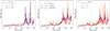 |
Fig. 1. Stochastic star formation histories (SFRsmooth × SFRstochastic) for different combinations of parameters generated with the STOCHASTICSFH module. Each panel shows the impact on the SFH of one specific parameter: σ (left panel), τbreak (middle panel), and α (right panel), in all cases the age and τmain are fix to 500 and 1000 Myr, respectively. |
Similar descriptions have also been used in the literature to model the SFH of galaxies at high redshift in physically-motivated approaches such as in Sun et al. (2025) and Kravtsov & Belokurov (2024), although in those studies the first term is associated with the mass accretion rate onto dark matter halos, so it is a mass-dependent function. Recently, Faisst & Morishita (2024) used this approach to model the fluctuations of galaxy SFRs around the MS at a given stellar mass and redshift. Following their study, we fix α to 2 and τbreak to 150 Myr as these parameters are found difficult to constrain from the observations (e.g., Caplar & Tacchella 2019). We note that these values do not prevent from modeling galaxies in lulling or temporary quenching phases, as shown by Faisst & Morishita (2024). This leaves two free parameters, σ and τmain, in addition to the galaxy age.
2.2. Test of the STOCHASTICSFH module
We test the ability of the STOCHASTICSFH module, combined with spectral population models, nebular models, and dust attenuation, to reproduce JWST observations of galaxies at z ≥ 6. In this test, we focus on constraining only the amplitude of the stochastic fluctuations (σ), since we fixed the other parameters of the STOCHASTICSFH module. However τmain is free to provide variations in the smooth component of the SFH.
We built a mock catalog of galaxies at 6 < z < 12 using the set of input parameters presented in Table 1, generating 105 simulated galaxies per σ. To compare with real observations, we computed the fluxes in the same set of filters as JADES (see Sect. 3; Eisenstein et al. 2023a), including 9 HST bands and 14 JWST/NIRCam bands. Then we perturbed the fluxes with a random Gaussian noise matching the sensitivity of JADES survey. In Fig. 2, we show color distributions of the simulated catalog with added noise for σ = 0.01, 0.1, 0.4, 0.8 compared to real observations (first column). The parameter range of the color distributions obtained with the simulated catalog is large enough to cover the observed colors for each burstiness level (σ), especially with σmock = 0.84. This first test ensures that the stochastic SFH, combined with typical SED modeling components, can reproduce a wide range of observed colors.
CIGALE input parameters used to build the mocks SEDs and to fit the spectrum of galaxies at z ≥ 6.
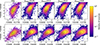 |
Fig. 2. Color-color diagram using JWST/NIRCam bands from the JADES catalog (left columns) and from the simulated catalogs (from second to last columns). These simulated catalogs are computed assuming, from left to right, σ of 0.01, 0.1, 0.4, and 0.8. The two different rows show the color-color diagram obtained with two different band combinations chosen to take into account redshift and parameter coverage to ease the comparison. The color lines show the contours that enclose the 16th, 50th, 84th, and 90th of the data in the observations. The implemented stochastic SFH can reproduce observed colors at z > 6. |
We used CIGALE to fit the simulated SEDs. For this test, we adopted the input parameters listed in Table 1, that is the same set of parameters that we used to fit the observations. It is important to emphasize that we constructed one mock catalog for each of the seven tested σmock values. Each of these catalogs is then independently fitted seven times, each time fixing σrun to a different value. This approach allows us to identify potential biases in the inferred SFHs when an inadequate model is used, as well as to assess the challenges in determining the best suited σrun.
The χ2 distributions for these different configurations are shown in Fig. 3. The distributions are narrow with a median value that depends on σrun. For all simulated catalogs, σrun = 0.8, a high level of burstiness, shows the best results in terms of χ2 distribution. In contrast, using σrun = 0.01 to fit galaxies’ SED that were built with bursty SFH results in poorer fit quality as probed by χ2 distribution. This indicates that a model with a smooth evolution lacks the flexibility to accurately describe bursty SFHs.
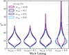 |
Fig. 3. χ2 obtained by fitting the mock catalogs with CIGALE. The different fits for each simulated catalog are color-coded by σrun used in the fit. A high level of burstiness (σrun ∼ 0.8) provides good fit quality, whatever the intrinsic level of burstiness of the fitted galaxy, while smoother SFHs struggle to fit bursty galaxy SEDs. |
We compare the SFR obtained through Bayesian-like analysis with CIGALE, with the true values from the mock catalogs. In Fig. 4, for each combination of σmock and σrun, we show the recovered SFR as a function of the true ones. Note that the SFHs simulated by CIGALE for the mock catalogs are normalized to 1 M⊙, making the resulting SFR values equivalent to the specific SFR (sSFR). The results suggest that the most bursty model (σrun = 0.8) provides a better recovery of the SFR due to its greater flexibility in capturing both high and low values. This effect is particularly evident for the mock catalog built using σmock = 0.8, shown in the bottom row. When a smooth model (dominated by a τ-delayed SFH, σrun = 0.01) is used to fit galaxies with a stochastic SFH, the median SFR of galaxies with very low SFR (< 2.5 × 10⁻¹¹ M⊙ yr−1) is overestimated by ∼1.3 dex. In contrast, when using the appropriate model, i.e., with (σrun = 0.8), this difference is reduced by ∼0.5 dex. At higher SFRs (> 4.3 × 10⁻⁸ M⊙ yr−1), we observe an underestimation of ∼0.5 dex when fitted with σrun = 0.01, which decreases to ∼0.25 dex when fitted with σrun = 0.8. Furthermore, the bias in SFR estimation tends to decrease from ∼0.7 dex to ∼0.3 dex when a bursty SFH model is used.
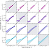 |
Fig. 4. Comparison between the mock SFR10 (true SFR10) and the SFR10 recovered by CIGALE (estimated SFR10) for all mock catalogs (rows) fitted with the different values of σrun (columns). The boxes span from the first quartile (Q1 = 25%) to the third quartile (Q3 = 75%), with a line indicating the median position, while the error bars extend from the 16th to the 84th percentile of the cumulative distribution. The gray background in the panels highlights when σrun match σmock. The SFH with the highest level of burstiness (σrun = 0.8) provides the best estimate of SFR10. |
These results show that the STOCHASTICSFH module implemented in CIGALE in this work is able to reproduce a broad range of SFH and SFRs. In contrast, the classic parametric τ-delayed model tends to overestimate the star formation rate and fails to capture extreme star-forming episodes, such as the bursts that galaxies at high redshift may undergo. It is important to note that this test was performed using the photometric filters covered in JADES (NIRCAM and HST). Including additional constraints, such as nebular emission lines such as Hα, although this is not accessible at our redshift range with JWST, is expected to further improve the accuracy of the results.
3. Observational data
We used the second data release5 (Program ID: 1180 and 1210, PIs: Eisenstein and Lützgendorf, respectively) of the JWST Advanced Deep Extragalactic Survey (JADES, Rieke et al. 2023; Bunker et al. 2024; Eisenstein et al. 2023b; Hainline et al. 2024), which cover ∼68 arcmin2 of the Hubble Ultra Deep Field, and presented in Eisenstein et al. (2023a). This catalog involves seven broad and five medium6 JWST/NIRCam bands from JADES (F090W, F115W, F150W, F200W, F277W, F335M, F356W, F410M, F430, F444W, F460M, and F480M), two medium NIRCam bands (F182M and F210M) from the JWST Extragalactic Medium-band Survey (JEMS, Williams et al. 2023) and First Reionization Spectroscopically Complete Observations (FRESCO, Oesch et al. 2023), and nine HST bands (5 ACS + 4 WFC3) from the Hubble Legacy Field (Illingworth et al. 2016). The source detection was performed in an inverse variance-weighted stack image of the long wavelength bands (F277W, F335M, F356W, F410M, and F444W images), and the photometry was measured in Kron aperture and six different circular apertures. Photometric redshifts are computed with the code EAZY (Brammer et al. 2008). The photometric redshifts have an average offset of 0.05 with a Δz/(1 + z) = 0.024 compared to a compilation of spectroscopic redshifts. For details on the data reduction process, photometry, and redshift estimates, we refer to Rieke et al. (2023), Eisenstein et al. (2023a), and Robertson et al. (2024).
We used the photometric catalog based on KRON (PSF-Convolved)7 apertures, restricted to NIRCam and HST/ACS bands, excluding ACS F850LP, as it is covered by the deeper NIRCam F090W data. HST/WFC3 photometry was not included due to its poor spatial resolution and low signal-to-noise ratio (S/N). The 5σ flux depths for the broad NIRCam bands range from 30.7 to 30.2 mag, while for the medium bands, they vary between 30.9 and 30.1 AB mag. We selected sources within 6 < z < 12 and imposed 23 mag < F277W < 30 mag cut to remove contamination from stars and noisy photometry. When available, we adopted the spectroscopic redshifts from the third JADES data release8 presented in D’Eugenio et al. (2025). This selection results in a final sample of 6730 galaxies within 6 < z < 12, 4369 objects at 6 < z < 7, 1717 at 7 < z < 9, and 644 at z > 9. Spectroscopic redshifts account for only 1% (73 sources) of the total sample.
4. SED modeling with stochastic SFH
In this section, we perform SED fitting of the selected JADES subsample using the stochastic SFH described in Sect. 2.1. Our goal is to test if a particular level of burstiness, characterized by σrun, is more suitable to model the emission of z > 6 galaxies and what its impact is on the estimated physical properties.
4.1. Burstiness and fit quality
We used CIGALE to fit HST+JWST photometry and derive physical properties. The fitting setup follows the approach described in Sect. 2.2. We performed independent CIGALE runs, each time varying the burstiness level (σrun = 0.01, 0.1, 0.4, 0.6, 0.8, 1.0), ranging from a classic τ-delayed SFH with negligible stochasticity (σrun ≲ 0.1) to a scenario dominated by strong bursts (σrun = 1.0). The input parameters used in the SED fitting are listed in Table 1.
In Fig. 5, we compare the χ2 distribution obtained for the different σrun values. The fit quality improves as the burstiness level increases. The distribution also becomes narrower at high σrun, reinforcing the preference for a stochastic SFH at high redshift. The median χ2 (white line in Fig. 5) saturates at ∼9 when σrun ≳ 0.8 is reached. The improvement of fit with increasing stochasticity is also found in individual redshift bins. These results confirm the conclusion obtained from the analysis of the mock catalogs: a high level of burstiness accounted for in the SFH is needed to fit early galaxies’ SED. This is also consistent with the conclusions of Faisst & Morishita (2024), who found that the best-fit parameter for galaxies at z ∼ 7 in the SPHINX20 simulation is σ ∼ 0.7. The improvement of the χ2 distribution is the results of the wider variation in the recent SFH allowed by the highly bursty SFH. However, even if these χ2 distributions show that models with high burstiness level are needed to fit properly the observations, a lower χ2 obtained by a more complex model is not necessarily significant statistically as shown in Aufort et al. (2020). Hence we do not rely on the χ2 distributions for our analysis in the rest of this work.
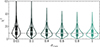 |
Fig. 5. χ2 distribution of the whole sample for each CIGALE run. The σrun used to model the SFH is indicated by the x-axis. The black dashed line shows the median χ2 for σrun = 0.8. The embedded box plot of each distribution indicates the median, interquartile range (IQR), and whiskers. A high level of burstiness accounted for in the SFH is needed to fit early galaxies’ SED. |
4.2. Impact of the SFH burstiness on the main sequence
We now investigate the impact of the level of burstiness on the derivation of physical properties. As an example, we show in Fig. 6 the best-fit SED obtained with CIGALE for a galaxy at z ∼ 6.3, for σrun = 0.01, 0.4, and 0.8. The model using high σrun provides a better fit of the observations, especially compared to the τ-delayed model (σrun = 0.01). Although, the number of free parameters is the same for each model, the χ2 obtained decreases significantly as σrun increases, dropping from 60.9 to 19.4 when comparing σrun = 0.01 and σrun = 0.8, respectively. The SED using τ-delayed SFH (σrun = 0.01) underestimates fluxes at < 2 μm and yields a redder UV β slope.
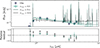 |
Fig. 6. Example SED of a galaxy at z ∼ 6 (top panel) and residuals (bottom panel). The dark purple squares are the fluxes from HST and JWST. The solid lines are the best-fit models obtained by CIGALE. The open circles indicate the modeled fluxes for the different models (in the top panels only for σrun = 0.8). |
When considering the full galaxy sample, we find that the choice of SFH affects the derived properties (see Appendix B). The stellar masses are higher by ∼0.1 dex when low σrun is assumed (≲0.1). At higher redshift, the rest-frame NIR emission is less constrained (see Appendix A for further details) and the difference in stellar mass between the different levels of burstiness becomes negligible. The SFRs are higher by ∼0.25 dex at 6 < z < 7 to ∼0.09 dex at 9 < z < 12 for σrun = 0.8. The UV β slope is slightly bluer for σrun = 0.8 compared to σrun = 0.01 at 6 < z < 9, while at z > 9, the median values are nearly identical. However, the stochastic SFH (σrun = 0.8) allows for a wider range of β values in all redshift bins.
To explore further the impact of the burstiness assumed by SFH models, we place the JADES galaxies of our sample in the SFR − M★ plane in Fig. 7. In the three redshift bins, the τ-delayed model (σrun = 0.01) results in a strong and tight correlation between the SFR and the stellar mass, even at high redshifts (z > 9). This is due to the fact that this model offers a limited range of SFR achievable (e.g., Ciesla et al. 2017). The dispersion around the MS increases with increasing σrun. In Table 2, we compute the Spearman coefficients for the full sample and for different SFH models. With σrun = 0.01, the correlation is very strong > 0.8 and reaches the high value of 0.9 in the 9 < z < 12 bin. Smooth SFH models impose a strong prior on sSFR, limiting the range of possible SFRs and producing a well-defined main sequence (Buat et al. 2014; Carnall et al. 2019). In Sect. 2.2, we observed similar trends when fitting the mock catalogs. Models with low burstiness levels lack flexibility, often leading to overestimated or underestimated SFRs in bursty galaxies. At higher burstiness level, the Spearman coefficient decreases with increasing σrun and increasing redshift. For σrun = 0.8, these coefficients are indicating a moderate to weak correlation between SFR and M★ at z ≥ 7 while the relation remains strong at z < 7. These results are consistent with Ciesla et al. (2024), who found similar coefficient ranges and trends with redshift, although using a nonparametric SFH (flat prior, linearly sampled time bins). Our results indicate that the MS scatter is strongly dependent on the choice of SFH model, which has already been discussed in the literature (e.g., Buat et al. 2014; Ciesla et al. 2017; Leja et al. 2022), and the level of burstiness modeled in it.
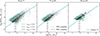 |
Fig. 7. SFR–M★ relation obtained from different burstiness levels in the SFH, color-coded by the assumed σrun. The dashed and dotted gray lines show when the classified sample (see Sect. 5) is 85% and 95% complete, respectively. The blue line shows the SFR–M★ from Popesso et al. (2023), converted from a Kroupa & Boily (2002) to a Chabrier (2003) IMF. The scatter of the MS strongly depends on the burstiness encoded in the assumed SFH. |
Spearman correlation coefficients for the SFR10 − M* plane with the different SFH models (σrun) in the three redshift bins.
5. SFH classification
We investigate whether the galaxies in our sample exhibit stochastic star formation, based on the result of the SED fitting assuming different burstiness. As explained in Sect. 1, there is increasing evidence from observations that galaxies at high redshift experience random periods of star formation (e.g., Dressler et al. 2024; Endsley et al. 2025; Ciesla et al. 2024; Langeroodi & Hjorth 2024; Cole et al. 2025). We first classify galaxies according to their preferred level of burstiness obtained from the SED fitting. We then select galaxies to build a mass-complete sample. We finally study the evolution of the fraction of bursty galaxies and their physical properties.
5.1. Galaxy classification with Bayes factor
We compare the quality of fit obtained from the CIGALE runs using the different levels of burstiness. We thus use the Bayes factor (BF) defined as:
 (4)
(4)
where p(xobs|m) is the likelihood integrated over the prior distribution for a given model m and observations xobs. We choose the model with σrun = 0.8, as our reference model, to be able to account for high burstiness, as smooth SFH models can not reproduce bursty galaxies, according to χ2 distribution (Fig. 5). The BF is then computed for each other model against this reference. We also implemented some model quality control: for each model, we first exclude observations for which the fit yields an effective sample size (neff) below 100. The effective sample size estimates how many independent samples effectively contribute to the posterior distribution approximation; a low neff indicates that the sampling process is inefficient and dominated by low-weight samples. In such cases, the likelihood is effectively informed by too few independent models and the resulting Monte Carlo approximation of the integral is poor.
We used σrun = 0.8 as reference and define it as “bursty SFH”. To be conservative, we define as “smooth” the run made with σrun = 0.01. We now divide galaxies in our sample in two groups: bursty galaxies (BFσrun = 0.8/σrun = 0.01 = BFBursty/Smooth > 3) and smooth galaxies (BFBursty/Smooth < 3), following the Jeffreys’ scale (see, e.g., Robert 2007; Aufort et al. 2020). For galaxies classified as smooth (BFBursty/Smooth < 3), we assign the physical properties obtained from the run with σrun = 0.01. This classification results in 30% (1970) of galaxies being identified as bursty and 70% (4600) as smooth in the whole sample. We test the impact of this classification by changing the reference burstiness model from σrun = 0.8 to σrun = 0.6, finding that the respective percentages vary by only ∼1%. In Appendix C, we test the classification method and examine the impact of the S/N and the choice of the BF threshold (BFBursty/Smooth > 3).
5.2. Mass-complete sample and physical properties
For the rest of the analysis, we need to determine the mass-completeness limit of our sample following the approach proposed by Pozzetti et al. (2010) (see also Florez et al. 2020; Mountrichas et al. 2022; Ciesla et al. 2024). We estimated the limiting stellar mass (log M★, lim) of each galaxy, defined as the stellar mass a galaxy would have if its apparent magnitude (mAB) were equal to the limiting magnitude of the survey (mAB, lim), log M★, lim = log M★ + 0.4 × (mAB − mAB, lim). This gives us the distribution of limiting stellar masses for our sample in each redshift bin. To define a representative mass-completeness limit, we selected the faintest 20% of galaxies in each redshift bin and computed the 80th and 95th percentiles of their log M★, lim distribution. In this work, we used the NIRCam/F277W filter and the selection cut we imposed in Sect. 3 as the limiting magnitude, 30 mag, which is brighter than the sensitivity of the survey, ∼30.7 mag (Eisenstein et al. 2023a). The limiting stellar mass could be affected by the choice of SFH. However, at z < 9, the difference in stellar mass between models is below 0.06 dex, and < 0.25 dex in the highest redshift bin. Our sample is 85% complete above log(M★, lim) = 7.73, 7.81, and 7.86 at 6 < z < 7, 7 < z < 9, and 9 < z < 12, respectively, and 95% complete above log(M★, lim) = 7.84, 7.92, and 8.0 in the same redshift bins (see Fig. 7). From now on, we only study galaxies with stellar masses above the limits, ensuring 95% mass-completeness. In Table 3, we provide the median properties of the mass-complete sample.
Properties derived from SED modeling of the mass-complete sample assuming σrun = 0.01, 0.4, and 0.8.
6. Evolution of galaxies’ burstiness
6.1. From the SFH classification
The fraction of galaxies in the two groups described in Sect. 5.1, bursty and smooth, evolves with redshift. In the left panel of Fig. 8, we show the fraction of high-mass galaxies (8.8 < log M★/M⊙ < 9.5) with a bursty SFH, according to the BF, as a function of redshift in the three redshift bins considered in this work. We choose this number to be 1 dex above the mass-completeness limit, to ensure a 100% complete sample. There is a tentative trend indicating an increasing fraction of high-mass galaxies with a bursty SFH with redshift. The trend is not clear between z ∼ 6.5 and z ∼ 8 with consistent median values, although the dispersion is smaller in the first redshift bin. At z > 8, the fraction of galaxies classified as bursty strongly increases with redshift. The overall trend is consistent with the results of Ciesla et al. (2024) obtained from a different method (distribution of the variations of the recent SFH using nonparametric models) on the same sample. To understand if the different rest-frame wavelength coverages due to redshift probed by the HST+JWST observations could bias our results in artificially creating this trend, we performed a second CIGALE run removing longer wavelength filters in galaxies with z < 11 in order to match the rest-frame wavelength coverage of galaxies at z = 11, although this is not ideal as the wavelength coverage of the filters is not homogeneous. In the right panel of Fig. 8, we show the resulting fractions of bursty galaxies obtained with this limited wavelength coverage. The trend is stronger, indicating that the difference in rest-frame coverage is not the origin of the decrease of the fraction of bursty galaxies with decreasing redshift.
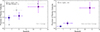 |
Fig. 8. Fraction of high-mass (8.8 < log M★/M⊙ < 9.5) galaxies classified as bursty as a function of redshift using the Bayes factor (see Sect. 5.1). The left panel shows the results when full spectral information at each redshift is used, while the right panel shows the results assuming the same rest-frame wavelength coverage as a galaxy at z = 11. Uncertainties on the fractions are derived from Poisson distribution, while uncertainties on the redshifts correspond to the 16th–84th percentile range of the redshift distribution within each stellar mass bin. The gray downside triangles show the fraction of stochastic massive galaxies (log M★ > 9) found in Ciesla et al. (2024), obtained from the variations of the recent SFR using nonparametric SFH. There is a trend showing an increasing fraction of bursty galaxies with increasing redshift that is not due to the difference in wavelength coverage. |
For galaxies with lower stellar masses (log M★/M⊙ < 8.8), we obtain a fraction of bursty galaxies lower than 20% at all redshifts. This could be surprising as it is expected that galaxies with lower stellar mass have more bursty SFH (e.g., Langeroodi et al. 2024). Low-mass galaxies are fainter with an average MUV of  mag in this mass bin compared to
  mag in the high-mass bin. Therefore, the uncertainties in the flux densities are larger: 15% on average in the JWST/F277W filter for the low-mass bin compared to 7% for the high-mass bin. To test whether this could be the origin of this low fraction of bursty sources, we use the best-fit models obtained with σrun = 0.8 as realistic simulated observations to evaluate how the classification is impacted by the S/N in Appendix C.1. We find that the fraction of bursty galaxies correctly identified drops from ∼70% at S/N ∼ 15 to ∼32% at S/N ∼ 7 (typical for the low-mass bin), implying that a large fraction of low-mass bursty systems can be misclassified by the BF analysis due to their low S/N. We note that this is partly driven by our conservative classification threshold (BFBursty/Smooth < 3), which is set to obtain a pure sample of bursty galaxies at ∼95% (see Appendix C.1). Hence, it is difficult to distinguish between models for faint sources from the BF analysis, as bursty and smooth SFH result in equivalently good χ2, confirming the importance of S/N in our analysis.
6.2. The log(SFR10/SFR100) ratio
Another way to probe the burstiness of galaxies’ star formation activity is to look at the ratio between the most recent SFR, for instance averaged over the last 10 Myr, and the SFR averaged over a longer timescale such as 100 Myr (e.g., Endsley et al. 2025; Langeroodi et al. 2024; Kokorev et al. 2025). The most recent SFR is traced by emission lines, while the longer timescales are probed by continuum. However, we only have access to spectroscopy for 1% of our sources. To understand if we recover log10(SFR10/SFR100) that are consistent with studies from the literature using spectroscopy, we show this ratio as a function of redshift in Fig. 9. We separate galaxies classified as having a smooth SFH from the bursty galaxies, and we highlight the median value of the ratio for bursty galaxies with enhanced SFR and bursty galaxies that underwent a decrease of their star formation activity. Overall, our estimates are in agreement with values from the literature obtained as statistical samples (Cole et al. 2025) or from individual sources (Arrabal Haro et al. 2023; Carniani et al. 2024; Castellano et al. 2024; Hsiao et al. 2024; Fujimoto et al. 2024; Napolitano et al. 2025; Kokorev et al. 2025). Galaxies of our samples tagged with smooth SFH show a slight decrease of the log10(SFR10/SFR100) ratio with decreasing redshift. This trend is consistent with those of Kokorev et al. (2025) at z > 14 and Cole et al. (2025) at z < 8, bridging these two relations. Galaxies classified as bursty with an enhanced SF activity (log10(SFR10/SFR100) > 0) have a typical ratio of ∼0.5 that is consistent with the individual sources at z > 10 as well as the relation from Kokorev et al. (2025). We do not see any significant decrease of the median log10(SFR10/SFR100) ratio with decreasing redshift for these galaxies. Interestingly, ∼12% of the galaxies in our sample that are classified as bursty show a negative log10(SFR10/SFR100) ratio, indicating that they recently underwent a rapid decrease of their SF activity. These galaxies are expected and consistent with individual sources that have been identified in the literature as lull or mini-quenched galaxies (Dome et al. 2024; Looser et al. 2024, 2025; Endsley et al. 2025; Covelo-Paz et al. 2025).
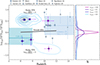 |
Fig. 9. Evolution of the log10(SFR10/SFR100) ratio, used as an indicator of burstiness, as a function of redshift. Blue contours indicate the distribution of the galaxies of our sample classified as having a bursty SFH. The big square and diamonds indicate the median value for each of the three redshift bins considered in this work for bursty galaxies with enhanced SF activity and decreasing activity, respectively. The black solid line is a linear fit to the ratio obtained for galaxies classified as having a smooth SFH. Measurements from the literature are also shown for comparison (Cole et al. 2025; Kokorev et al. 2025; Carniani et al. 2024). The SFR10/SFR100 ratio from Arrabal Haro et al. (2023), Castellano et al. (2024), Hsiao et al. (2024), Bunker et al. (2023), Álvarez-Márquez et al. (2025), Fujimoto et al. (2024), Napolitano et al. (2025) were taken from Kokorev et al. (2025). The light blue shaded regions represent the log10(SFR10/SFR100) distribution within 1-σ for bright galaxies (MUV < −20; Kokorev et al. 2025) and the 16th–84th percentiles from Cole et al. (2025), with the median indicated by the solid line. The right panel shows the distribution of log10(SFR10/SFR100) ratios obtained from the simulated mock catalogs with different burstiness levels presented in Sect. 2.2. The ratio is constant as a function of redshift. Only high ratios of ≳0.2 cannot be reproduced by a smooth SFH. |
In Fig. 9, we place our results for the JADES sample along with measurements from the literature using different surveys and different types of data (photometric and/or spectroscopic). In these studies, the log10(SFR10/SFR100) parameter is used as an indicator of burstiness and galaxies with log10(SFR10/SFR100) > 0 are classified as bursty (Endsley et al. 2025; Kokorev et al. 2025). Gathering a sample of 12 galaxies at z > 10 with spectroscopic information, Kokorev et al. (2025) found a mean log10(SFR10/SFR100) of 0.30 ± 0.02 dex and a scatter of 0.42 ± 0.02 dex around this value. At lower redshift, 4 < z < 6, Cole et al. (2025) obtained a mean value of ∼ − 0.21 with a large scatter of 0.46. The combination of these results would point toward a decrease of the burstiness of galaxies with decreasing redshift. We use the simulated mock sample of galaxies presented in Sect. 2.2 with different σmock values to derive the distributions of log10(SFR10/SFR100) and show them in the right panel of Fig. 9. A pure τ-delayed SFH only yields a narrow distribution of log10(SFR10/SFR100) around 0. However, an SFH with a low level of burstiness σmock = 0.1 (see Fig. 1) can produce a distribution with SFH models reaching log10(SFR10/SFR100) values of ±0.3. Values exceeding these limits can only be reproduced by bursty SFH models. Hence, a positive value of log10(SFR10/SFR100) does not necessarily imply a bursty SFH if the value is close to 0 (±0.2−0.3), but a higher ratio would definitely rule out a smooth SFH.
To investigate a possible evolution of the burstiness level of the galaxies in our sample, we compute the fraction of massive galaxies (8.8 < log M★/M⊙ < 9.5), for consistency with the previous section, that have a log10(SFR10/SFR100) larger than 0.2. At z > 9, no massive sources have a ratio larger than 0.2. However, we obtain a fraction of 0.28 ± 0.06 and 0.38 ± 0.11, at 6 < z < 7 and 7 < z < 9, respectively. Although the Poissonian errors are large, especially at 7 < z < 9, these numbers point toward an increasing fraction of bursty galaxies with increasing redshift, confirming the results of the previous section.
7. Evolution of σUV
In the literature, σUV is defined as the dispersion in mag around a median MUV obtained from a MUV − Mhalo relation and has been used to quantify the stochasticity of star formation (Shen et al. 2023; Shuntov et al. 2025a). To compute σUV, we used the complete sample and estimated the median MUV in bins of stellar masses to remove the trend between MUV and M★. We normalized MUV using the corresponding median value of their stellar mass bin and computed the dispersion of the corrected MUV distribution. To account for uncertainties, we perform Monte Carlo realizations of both M★ and MUV by drawing from Gaussian using the uncertainties from the SED fitting as the width of the distribution. In each realization, we apply the binning, normalization, and compute the scatter of the corrected MUV distribution. The final value of σUV and its uncertainties are estimated from the percentiles of the resulting distribution. We obtain σUV of 0.72 ± 0.02, 0.54 ± 0.02, and 0.57 ± 0.03 mag, at 6 < z < 7, 7 < z < 9, and 9 < z < 12, respectively. We compare these values with results from the literature in Fig. 10.
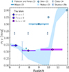 |
Fig. 10. Evolution of σUV with the redshift for our sample in JADES at 6 < z < 12. The uncertainties on σUV are estimated from bootstrapping. The error bar on redshifts indicates the 16th to 84th percentiles of the distributions. The blue shades and markers show estimations from the literature, which are based on semi-analytical models and simulations (Pallottini & Ferrara 2023; Shen et al. 2023; Muñoz et al. 2023; Mason et al. 2023) or observations (Ciesla et al. 2024; Shuntov et al. 2025a). Our estimate σUV is consistent with the literature and too low to explain the mild evolution of the UVLF at z > 10 only from bursty SFH, as estimated by Shen et al. (2023) (empty circles) using empirical models. |
Our measurements of σUV show relatively good agreement with previous results at z ∼ 6 − 12. Ciesla et al. (2024) performed a similar analysis using SED modeling with a nonparametric SFH, and found ∼0.6 mag higher values when derived from the MUV distribution. However, in their measurement, they took into account all galaxies with log M★/M⊙ ≥ 9, hence considering one mass bin. For this reason, their values can be considered as upper limits. A different observational approach is used in Shuntov et al. (2025a), where a spectroscopic sample was used to constrain the MUV − Mh, the relation between star formation efficiency (SFE) and Mh, stochasticity and galaxy bias. Our results are consistent within their uncertainties. Muñoz et al. (2023) followed similar semi-empirical models to fit the UVLF and derived σUV. They found low values < 0.8 mag, which match our results, followed by a sharp increase at z ∼ 10 that can still be compatible with our results, although our high-z bin value is low. Interestingly, at lower redshifts, our measurements follow well their predicted redshift dependence of σUV. Mason et al. (2023) used empirical models to study the MUV − Mh relation and the impact of young bright galaxies in the UVLF, which are the most likely to dominate the observations, and showed an upscatter up to 1.5 mag above the median relation. With our observations at the same redshift range, we observe a lower level of stochasticity in our σUV measurements. In the SERRA simulations, Pallottini & Ferrara (2023) found σUV = 0.61 mag at z ∼ 7.7, which is consistent with our results. Finally, Shen et al. (2023) showed that to explain the observed UVLF at z > 10, values as high as σUV > 1.5 mag would be required. Our level of stochasticity, as probed by σUV is not high enough to explain the observed UVLF.
Our results do not indicate an increase in σUV that some works find necessary to describe the high-z UVLF and thus reinforce the idea of a solution combining several effects in addition to bursty SFH. A high SFE has been found to play a role in the mild evolution of the UVLF at z > 10 as discussed and found by Gelli et al. (2024) and Shuntov et al. (2025a). Here, we used our results, particularly the SFR obtained from specific modeling of the SFH to have a first order estimate of the instantaneous SFE (ϵ9, note that is different from the integrated star formation efficiency ϵ★) by assuming the stellar-to-halo mass relation (SHMR) from Shuntov et al. (2025b). They inferred it using nonparametric abundance matching of their stellar mass function (SMF) and the Watson et al. (2013) halo mass function (HMF). This allowed us to estimate the halo mass of our sample, then compute the halo accretion rate Ṁh following Dekel et al. (2013), which is well understood from ΛCDM, and it is a function of halo mass and redshift. Finally, we estimated ϵ from:
 (5)
(5)
where fb ≈ 0.16 is the baryon fraction (Moster et al. 2018; Tacchella et al. 2018), and SFR is the derived SFR10 from the SED modeling. Our galaxies are hosted in halos of median (range) log(Mh/M⊙) = 10.75 ± 0.01 (10.62 − 11.44), 10.56 ± 0.01 (10.38 − 11.11), and 10.51 ± 0.02 (10.40 − 10.92) at 6 < z < 7, 7 < z < 9, and 9 < z < 12, respectively. We tested the impact of a different SHMR by using the UNIVERSEMCHINE simulation suite (Behroozi et al. 2019). We found consistent results, except at z > 9, which is possibly due to the fact that this simulation suite was calibrated using pre-JWST observations.
In Fig. 11, we show our derived ϵ as a function of Mh for our sample covering the low-mass end (log(Mh/M⊙) < 11.4). We do not observe any strong evolution with redshift and obtain a median ϵ of 0.06 ± 0.01, 0.06 ± 0.01, and 0.05 ± 0.01 at 6 < z < 7, 7 < z < 9, and 9 < z < 12, respectively. We compare our results with the observational measurements from Shuntov et al. (2025b), who, using a different approach based on halo occupation distribution (HOD) and the UVLF, found a variation of ϵ with halo mass consistent with our estimates. At z < 7, our measurements agree within 0.02 dex, while at 7 < z < 9, our ϵ values are approximately 0.1 dex higher. Our results on the SFE, shown in Fig. 11, do not suggest a significant (if any) increase in SFE in halos of log M ∼ 10.3 − 10.8, which combined with the measured values of σUV, seems unlikely to explain the slow evolution of the observed UVLF at high-z (e.g., Shen et al. 2023; Gelli et al. 2024; Shuntov et al. 2025a). However, we note that it is necessary to constrain the shape of the SFE–Mh relation over a sufficiently large halo mass range (about > 2 dex) and constrain the position of the peak (if any) as the shape of the SFE–Mh relation is more important than the peak value in the resulting UVLF (e.g., Feldmann et al. 2023). Currently, our sample is too small to constrain the shape of the SFE–Mh relation. Extending this work at both the fainter and brighter end will be crucial. Nonetheless, our inferred values for the SFE and σUV add further evidence that a combination with other mechanisms is likely responsible for the high-z UVLF such as a negligible dust attenuation (e.g., Ferrara et al. 2023), evolving top-heavy IMF (e.g., Hutter et al. 2025), or locally varying SFE modulated by gas cloud density (e.g., Somerville et al. 2025).
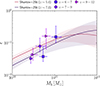 |
Fig. 11. Instantaneous star formation efficiency as a function of halo mass for the three redshift bins in our sample. Solid lines and shaded regions show the estimates from Shuntov et al. (2025a), based on the UV luminosity function and halo occupation distribution (HOD) modeling. Our estimates of ϵ do not show any strong variation with redshift and confirm the low values obtained by Shuntov et al. (2025a). |
8. Conclusion
The aim of this work is to model the SFH of high redshift galaxies (6 < z < 12) by testing different levels of stochasticity in the SFH assumption, and study the evolution of galaxies’ burstiness, in order to put constraints on the UV dispersion at these redshifts. To do so, we implemented and tested a stochastic SFH to reproduce the emission of high redshift galaxies.
-
By following the approach described in Caplar & Tacchella (2019), we modeled SFR fluctuations with time series that are computed through correlated Gaussian random numbers, defined by a PSD (see also Faisst & Morishita 2024). This approach is implemented in the SED modeling code CIGALE and allows to well reproduce the colors of observed galaxies at 6 < z < 12.
-
Using a simulated set of galaxies’ SEDs, we find that assuming a high level of stochasticity (quantified by σrun) for the SFH results in better fit quality (based on χ2 distributions) than a smooth SFH assumption (close to τ-delayed SFH), especially for highly bursty galaxies. This result is confirmed when applied on real observations from the JADES sample.
-
Comparing galaxies’ properties obtained for different levels of stochasticity on the SFR-stellar mass plane, we find that a smooth SFH results in a very tight relation between SFR and stellar mass at z ≥ 6 while the scatter of the relation increases with increasing level of stochasticity up to yield a weak relation at z > 7 (from a Spearman test). This highlights again the importance of SFH assumptions in constraining galaxies MS, as already found in the literature.
Having run CIGALE on the JADES galaxies assuming successively different levels of burstiness, we determined the best-suited SFH for each galaxy through a Bayes factor analysis. According to this, galaxies are classified as either smooth, and their physical properties are those obtained with quasi τ-delayed SFH (σrun = 0.01), or bursty, and the results of the run using a high stochasticity level are used (σrun = 0.8). After selecting a mass-complete sample, we find that:
-
For massive galaxies (8.8 < log M★/M⊙ < 9.5), the fraction of bursty galaxies increases from 0.38 ± 0.08 to 0.77 ± 0.2 with increasing redshift. This trend is not due to biases originating from differences in terms of rest-frame wavelength coverage, as using the same rest-frame coverage results in a steeper increasing trend.
-
Although we expect low-mass galaxies to be more bursty, only ≲20% of them are classified as bursty at all redshifts. This low fraction is attributed to observational bias, as they are faint, the S/N of the fluxes is low, and it is harder to significantly select a bursty SFH as more suitable from a Bayes factor analysis.
-
For bursty galaxies, we find no evolution with redshift of the log10(SFR10/SFR100) ratio, another indicator of burstiness. Galaxies classified as having a smooth SFH show a weak trend of decreasing ratio with decreasing redshift. Our measurements are consistent with previous estimates from the literature. However, the fraction of galaxies with log10(SFR10/SFR100) > 0.2 increases from 0.28 ± 0.06 to 0.38 ± 0.11 at z ∼ 6 and z ∼ 9, respectively.
-
We provide constraints on σUV derived from the MUV distribution in stellar mass bins. We obtain σUV of 0.72 ± 0.02, 0.54 ± 0.02, and 0.57 ± 0.03 mag at 6 < z < 7, 7 < z < 9, and 9 < z < 12, respectively. These values are consistent with Shuntov et al. (2025a) results based on observations and the estimates of Pallottini & Ferrara (2023) and Muñoz et al. (2023), confirming that bursty SFH alone is not responsible for the mild evolution of the UVLF at z > 10.
-
Assuming a stellar-to-halo mass relation, we use our estimated SFR to put constraints on the SFE, ϵ, and obtain 0.06 ± 0.01, 0.06 ± 0.01, and 0.05 ± 0.01 at 6 < z < 7, 7 < z < 9, and 9 < z < 12, respectively.
Although these results need to be confirmed with a spectroscopic sample, large enough to be statistically significant, the σUV and SFE values estimated in this work add further evidence that a combination with other mechanisms is likely responsible for the high-z UVLF. Other proposed solutions, such as a negligible dust attenuation (e.g., Ferrara et al. 2023), evolving top-heavy IMF (e.g., Hutter et al. 2025), or locally varying SFE modulated by gas cloud density (e.g., Somerville et al. 2025), must be explored.
In CIGALE, the age of a galaxy is the time since the birth of its first star.
Hereafter, we use the subscript “mock” to refer to mock catalogs generated with a given value of σ, and “run” to indicate the use of a fixed σ value in the SED fitting process with CIGALE.
F430M, F460M, and F480M images were acquired by JEMS but reprocess and release by JADES.
The photometry was extracted in PSF-matched images convolved with NIRCAM F444W PSF.
The third JADES data release for GOODS-S expanded the NIRSpec dataset through program PI:1210, providing over 2000 redshift measurements. However, this release does not include photometric data for GOODS-S.
The instantaneous SFE is different from the integrated SFE ( ).
).
Acknowledgments
The authors thank the anonymous referee for their valuable comments and suggestions, which helped improve the clarity and quality of this work. The authors are grateful to Guilaine Lagache for her insightful discussions and guidance. This work received support from the French government under the France 2030 investment plan, as part of the Initiative d’Excellence d’Aix-Marseille Université – A*MIDEX AMX-22-RE-AB-101. This work was partially supported by the “PHC GERMAINE DE STAEL” programme (project number: 52217VG), funded by the French Ministry for Europe and Foreign Affairs, the French Ministry for Higher Education and Research, the Swiss Academy of Technical Sciences (SATW) and the State Secretariat for Education, Research and Innovation (SERI). MB acknowledges support from the ANID BASAL project FB210003, supported by the French government through the France 2030 investment plan managed by the National Research Agency (ANR), as part of the Initiative of Excellence of Université Côte d’Azur under reference number ANR-15-IDEX-01. OI and LC acknowledge the funding of the French Agence Nationale de la Recherche for the project iMAGE (grant ANR-22-CE31-0007). This work has received funding from the Swiss State Secretariat for Education, Research and Innovation (SERI) under contract number MB22.00072, as well as from the Swiss National Science Foundation (SNSF) through project grant 200020_207349.
References
- Adams, N. J., Conselice, C. J., Austin, D., et al. 2024, ApJ, 965, 169 [NASA ADS] [CrossRef] [Google Scholar]
- Allen, M., Behroozi, P., & Ma, C.-P. 2019, MNRAS, 488, 4916 [NASA ADS] [CrossRef] [Google Scholar]
- Álvarez-Márquez, J., Crespo Gómez, A., Colina, L., et al. 2025, A&A, 695, A250 [NASA ADS] [CrossRef] [EDP Sciences] [Google Scholar]
- Arango-Toro, R. C., Ciesla, L., Ilbert, O., et al. 2023, A&A, 675, A126 [NASA ADS] [CrossRef] [EDP Sciences] [Google Scholar]
- Arrabal Haro, P., Dickinson, M., Finkelstein, S. L., et al. 2023, ApJ, 951, L22 [NASA ADS] [CrossRef] [Google Scholar]
- Astropy Collaboration (Price-Whelan, A. M., et al.) 2022, ApJ, 935, 167 [NASA ADS] [CrossRef] [Google Scholar]
- Aufort, G., Ciesla, L., Pudlo, P., & Buat, V. 2020, A&A, 635, A136 [NASA ADS] [CrossRef] [EDP Sciences] [Google Scholar]
- Bagley, M. B., Finkelstein, S. L., Rojas-Ruiz, S., et al. 2024, ApJ, 961, 209 [NASA ADS] [CrossRef] [Google Scholar]
- Baker, W. M., D’Eugenio, F., Maiolino, R., et al. 2025, A&A, 697, A90 [NASA ADS] [CrossRef] [EDP Sciences] [Google Scholar]
- Basu, A., Bhagwat, A., Ciardi, B., & Costa, T. 2025, arXiv e-prints [arXiv:2501.18559] [Google Scholar]
- Behroozi, P. S., Conroy, C., & Wechsler, R. H. 2010, ApJ, 717, 379 [Google Scholar]
- Behroozi, P. S., Wechsler, R. H., & Conroy, C. 2013, ApJ, 770, 57 [NASA ADS] [CrossRef] [Google Scholar]
- Behroozi, P., Wechsler, R. H., Hearin, A. P., & Conroy, C. 2019, MNRAS, 488, 3143 [NASA ADS] [CrossRef] [Google Scholar]
- Boquien, M., Burgarella, D., Roehlly, Y., et al. 2019, A&A, 622, A103 [NASA ADS] [CrossRef] [EDP Sciences] [Google Scholar]
- Bouwens, R. J., Illingworth, G. D., Oesch, P. A., et al. 2015, ApJ, 803, 34 [Google Scholar]
- Bouwens, R. J., Stefanon, M., Oesch, P. A., et al. 2019, ApJ, 880, 25 [NASA ADS] [CrossRef] [Google Scholar]
- Bouwens, R. J., Oesch, P. A., Stefanon, M., et al. 2021, AJ, 162, 47 [NASA ADS] [CrossRef] [Google Scholar]
- Bowler, R. A. A., Jarvis, M. J., Dunlop, J. S., et al. 2020, MNRAS, 493, 2059 [Google Scholar]
- Brammer, G. B., van Dokkum, P. G., & Coppi, P. 2008, ApJ, 686, 1503 [Google Scholar]
- Bruzual, G., & Charlot, S. 2003, MNRAS, 344, 1000 [NASA ADS] [CrossRef] [Google Scholar]
- Buat, V., Heinis, S., Boquien, M., et al. 2014, A&A, 561, A39 [NASA ADS] [CrossRef] [EDP Sciences] [Google Scholar]
- Bunker, A. J., Saxena, A., Cameron, A. J., et al. 2023, A&A, 677, A88 [NASA ADS] [CrossRef] [EDP Sciences] [Google Scholar]
- Bunker, A. J., Cameron, A. J., Curtis-Lake, E., et al. 2024, A&A, 690, A288 [NASA ADS] [CrossRef] [EDP Sciences] [Google Scholar]
- Calzetti, D., Armus, L., Bohlin, R. C., et al. 2000, ApJ, 533, 682 [NASA ADS] [CrossRef] [Google Scholar]
- Caplar, N., & Tacchella, S. 2019, MNRAS, 487, 3845 [NASA ADS] [CrossRef] [Google Scholar]
- Carnall, A. C., Leja, J., Johnson, B. D., et al. 2019, ApJ, 873, 44 [Google Scholar]
- Carniani, S., Hainline, K., D’Eugenio, F., et al. 2024, Nature, 633, 318 [CrossRef] [Google Scholar]
- Castellano, M., Fontana, A., Treu, T., et al. 2022, ApJ, 938, L15 [NASA ADS] [CrossRef] [Google Scholar]
- Castellano, M., Napolitano, L., Fontana, A., et al. 2024, ApJ, 972, 143 [Google Scholar]
- Chabrier, G. 2003, PASP, 115, 763 [Google Scholar]
- Ciesla, L., Charmandaris, V., Georgakakis, A., et al. 2015, A&A, 576, A10 [NASA ADS] [CrossRef] [EDP Sciences] [Google Scholar]
- Ciesla, L., Elbaz, D., & Fensch, J. 2017, A&A, 608, A41 [NASA ADS] [CrossRef] [EDP Sciences] [Google Scholar]
- Ciesla, L., Gómez-Guijarro, C., Buat, V., et al. 2023, A&A, 672, A191 [NASA ADS] [CrossRef] [EDP Sciences] [Google Scholar]
- Ciesla, L., Elbaz, D., Ilbert, O., et al. 2024, A&A, 686, A128 [NASA ADS] [CrossRef] [EDP Sciences] [Google Scholar]
- Ciesla, L., Adscheid, S., Magnelli, B., et al. 2025, A&A, 700, A277 [NASA ADS] [CrossRef] [EDP Sciences] [Google Scholar]
- Clarke, L., Shapley, A. E., Sanders, R. L., et al. 2024, ApJ, 977, 133 [NASA ADS] [CrossRef] [Google Scholar]
- Cochrane, R. K., Katz, H., Begley, R., Hayward, C. C., & Best, P. N. 2025, ApJ, 978, L42 [Google Scholar]
- Cole, J. W., Papovich, C., Finkelstein, S. L., et al. 2025, ApJ, 979, 193 [Google Scholar]
- Connolly, S. D. 2016, Astrophysics Source Code Library [record ascl:1602.012] [Google Scholar]
- Covelo-Paz, A., Meuwly, C., Oesch, P. A., et al. 2025, A&A, in press, https://doi.org/10.1051/0004-6361/202556119 [Google Scholar]
- Cueto, E. R., Hutter, A., Dayal, P., et al. 2024, A&A, 686, A138 [NASA ADS] [CrossRef] [EDP Sciences] [Google Scholar]
- Daddi, E., Dickinson, M., Morrison, G., et al. 2007, ApJ, 670, 156 [NASA ADS] [CrossRef] [Google Scholar]
- Dayal, P., Dunlop, J. S., Maio, U., & Ciardi, B. 2013, MNRAS, 434, 1486 [NASA ADS] [CrossRef] [Google Scholar]
- Dekel, A., Zolotov, A., Tweed, D., et al. 2013, MNRAS, 435, 999 [Google Scholar]
- D’Eugenio, F., Cameron, A. J., Scholtz, J., et al. 2025, ApJS, 277, 4 [Google Scholar]
- Dome, T., Tacchella, S., Fialkov, A., et al. 2024, MNRAS, 527, 2139 [Google Scholar]
- Donnan, C. T., McLeod, D. J., McLure, R. J., et al. 2023a, MNRAS, 520, 4554 [NASA ADS] [CrossRef] [Google Scholar]
- Donnan, C. T., McLeod, D. J., Dunlop, J. S., et al. 2023b, MNRAS, 518, 6011 [Google Scholar]
- Donnan, C. T., Dickinson, M., Taylor, A. J., et al. 2025, ApJ, 993, 224 [Google Scholar]
- Dressler, A., Rieke, M., Eisenstein, D., et al. 2024, ApJ, 964, 150 [NASA ADS] [CrossRef] [Google Scholar]
- Eisenstein, D. J., Johnson, B. D., Robertson, B., et al. 2023a, arXiv e-prints [arXiv:2310.12340] [Google Scholar]
- Eisenstein, D. J., Willott, C., Alberts, S., et al. 2023b, arXiv e-prints [arXiv:2306.02465] [Google Scholar]
- Elbaz, D., Daddi, E., Le Borgne, D., et al. 2007, A&A, 468, 33 [NASA ADS] [CrossRef] [EDP Sciences] [Google Scholar]
- Emami, N., Siana, B., Weisz, D. R., et al. 2019, ApJ, 881, 71 [NASA ADS] [CrossRef] [Google Scholar]
- Endsley, R., Chisholm, J., Stark, D. P., Topping, M. W., & Whitler, L. 2025, ApJ, 987, 189 [Google Scholar]
- Faisst, A. L., & Morishita, T. 2024, ApJ, 971, 47 [NASA ADS] [CrossRef] [Google Scholar]
- Faisst, A. L., Capak, P. L., Emami, N., Tacchella, S., & Larson, K. L. 2019, ApJ, 884, 133 [NASA ADS] [CrossRef] [Google Scholar]
- Feldmann, R., Quataert, E., Faucher-Giguère, C.-A., et al. 2023, MNRAS, 522, 3831 [NASA ADS] [CrossRef] [Google Scholar]
- Ferrara, A., Pallottini, A., & Dayal, P. 2023, MNRAS, 522, 3986 [NASA ADS] [CrossRef] [Google Scholar]
- Finkelstein, S. L., & Bagley, M. B. 2022, ApJ, 938, 25 [NASA ADS] [CrossRef] [Google Scholar]
- Finkelstein, S. L., Ryan, R. E., Papovich, C., et al. 2015, ApJ, 810, 71 [NASA ADS] [CrossRef] [Google Scholar]
- Finkelstein, S. L., Bagley, M., Song, M., et al. 2022a, ApJ, 928, 52 [CrossRef] [Google Scholar]
- Finkelstein, S. L., Bagley, M. B., Arrabal Haro, P., et al. 2022b, ApJ, 940, L55 [NASA ADS] [CrossRef] [Google Scholar]
- Finkelstein, S. L., Leung, G. C. K., Bagley, M. B., et al. 2024, ApJ, 969, L2 [NASA ADS] [CrossRef] [Google Scholar]
- Florez, J., Jogee, S., Sherman, S., et al. 2020, MNRAS, 497, 3273 [NASA ADS] [CrossRef] [Google Scholar]
- Fujimoto, S., Wang, B., Weaver, J. R., et al. 2024, ApJ, 977, 250 [NASA ADS] [CrossRef] [Google Scholar]
- Gelli, V., Salvadori, S., Ferrara, A., Pallottini, A., & Carniani, S. 2023, ApJ, 954, L11 [NASA ADS] [CrossRef] [Google Scholar]
- Gelli, V., Mason, C., & Hayward, C. C. 2024, ApJ, 975, 192 [NASA ADS] [CrossRef] [Google Scholar]
- Gelli, V., Pallottini, A., Salvadori, S., et al. 2025, ApJ, 985, 126 [Google Scholar]
- Hainline, K. N., Johnson, B. D., Robertson, B., et al. 2024, ApJ, 964, 71 [CrossRef] [Google Scholar]
- Harikane, Y., Ouchi, M., Oguri, M., et al. 2023, ApJS, 265, 5 [NASA ADS] [CrossRef] [Google Scholar]
- Hopkins, P. F., Gurvich, A. B., Shen, X., et al. 2023, MNRAS, 525, 2241 [NASA ADS] [CrossRef] [Google Scholar]
- Hsiao, T. Y.-Y., Abdurro’uf, Coe, D., et al. 2024, ApJ, 973, 8 [NASA ADS] [CrossRef] [Google Scholar]
- Hutter, A., Cueto, E. R., Dayal, P., et al. 2025, A&A, 694, A254 [NASA ADS] [CrossRef] [EDP Sciences] [Google Scholar]
- Illingworth, G., Magee, D., Bouwens, R., et al. 2016, arXiv e-prints [arXiv:1606.00841] [Google Scholar]
- Inoue, A. K. 2011, MNRAS, 415, 2920 [NASA ADS] [CrossRef] [Google Scholar]
- Iyer, K., & Gawiser, E. 2017, ApJ, 838, 127 [NASA ADS] [CrossRef] [Google Scholar]
- Iyer, K. G., Gawiser, E., Faber, S. M., et al. 2019, ApJ, 879, 116 [NASA ADS] [CrossRef] [Google Scholar]
- Kimm, T., & Cen, R. 2014, ApJ, 788, 121 [NASA ADS] [CrossRef] [Google Scholar]
- Kokorev, V., Chávez Ortiz, Ó. A., Taylor, A. J., et al. 2025, ApJ, 988, L10 [Google Scholar]
- Kravtsov, A., & Belokurov, V. 2024, arXiv e-prints [arXiv:2405.04578] [Google Scholar]
- Kroupa, P., & Boily, C. M. 2002, MNRAS, 336, 1188 [Google Scholar]
- Langeroodi, D., & Hjorth, J. 2024, arXiv e-prints [arXiv:2404.13045] [Google Scholar]
- Langeroodi, D., Hjorth, J., Ferrara, A., & Gall, C. 2024, arXiv e-prints [arXiv:2410.14671] [Google Scholar]
- Leja, J., Carnall, A. C., Johnson, B. D., Conroy, C., & Speagle, J. S. 2019, ApJ, 876, 3 [Google Scholar]
- Leja, J., Speagle, J. S., Ting, Y.-S., et al. 2022, ApJ, 936, 165 [NASA ADS] [CrossRef] [Google Scholar]
- Looser, T. J., D’Eugenio, F., Maiolino, R., et al. 2024, Nature, 629, 53 [Google Scholar]
- Looser, T. J., D’Eugenio, F., Maiolino, R., et al. 2025, A&A, 697, A88 [NASA ADS] [CrossRef] [EDP Sciences] [Google Scholar]
- Lower, S., Narayanan, D., Leja, J., et al. 2020, ApJ, 904, 33 [NASA ADS] [CrossRef] [Google Scholar]
- Ma, X., Hopkins, P. F., Garrison-Kimmel, S., et al. 2018, MNRAS, 478, 1694 [NASA ADS] [CrossRef] [Google Scholar]
- Mashian, N., Oesch, P. A., & Loeb, A. 2016, MNRAS, 455, 2101 [CrossRef] [Google Scholar]
- Mason, C. A., Trenti, M., & Treu, T. 2023, MNRAS, 521, 497 [NASA ADS] [CrossRef] [Google Scholar]
- Matteri, A., Ferrara, A., & Pallottini, A. 2025, A&A, 701, A186 [NASA ADS] [CrossRef] [EDP Sciences] [Google Scholar]
- McClymont, W., Tacchella, S., D’Eugenio, F., et al. 2025, MNRAS, 540, 190 [Google Scholar]
- Moster, B. P., Naab, T., & White, S. D. M. 2018, MNRAS, 477, 1822 [Google Scholar]
- Mountrichas, G., Buat, V., Yang, G., et al. 2022, A&A, 663, A130 [NASA ADS] [CrossRef] [EDP Sciences] [Google Scholar]
- Muñoz, J. B., Mirocha, J., Furlanetto, S., & Sabti, N. 2023, MNRAS, 526, L47 [CrossRef] [Google Scholar]
- Naidu, R. P., Oesch, P. A., van Dokkum, P., et al. 2022, ApJ, 940, L14 [NASA ADS] [CrossRef] [Google Scholar]
- Napolitano, L., Castellano, M., Pentericci, L., et al. 2025, A&A, 693, A50 [NASA ADS] [CrossRef] [EDP Sciences] [Google Scholar]
- Noeske, K. G., Weiner, B. J., Faber, S. M., et al. 2007, ApJ, 660, L43 [CrossRef] [Google Scholar]
- Oesch, P. A., Bouwens, R. J., Illingworth, G. D., Labbé, I., & Stefanon, M. 2018, ApJ, 855, 105 [Google Scholar]
- Oesch, P. A., Brammer, G., Naidu, R. P., et al. 2023, MNRAS, 525, 2864 [NASA ADS] [CrossRef] [Google Scholar]
- Oke, J. B., & Gunn, J. E. 1983, ApJ, 266, 713 [NASA ADS] [CrossRef] [Google Scholar]
- Pallottini, A., & Ferrara, A. 2023, A&A, 677, L4 [NASA ADS] [CrossRef] [EDP Sciences] [Google Scholar]
- Papovich, C., Cole, J. W., Yang, G., et al. 2023, ApJ, 949, L18 [NASA ADS] [CrossRef] [Google Scholar]
- Popesso, P., Concas, A., Cresci, G., et al. 2023, MNRAS, 519, 1526 [Google Scholar]
- Pozzetti, L., Bolzonella, M., Zucca, E., et al. 2010, A&A, 523, A13 [NASA ADS] [CrossRef] [EDP Sciences] [Google Scholar]
- Ren, K., Trenti, M., & Mason, C. A. 2019, ApJ, 878, 114 [Google Scholar]
- Rieke, M. J., Robertson, B., Tacchella, S., et al. 2023, ApJS, 269, 16 [NASA ADS] [CrossRef] [Google Scholar]
- Robert, C. P. 2007, The Bayesian Choice: From Decision-Theoretic Foundations to Computational Implementation (Springer) [Google Scholar]
- Robertson, B., Johnson, B. D., Tacchella, S., et al. 2024, ApJ, 970, 31 [NASA ADS] [CrossRef] [Google Scholar]
- Saxena, A., Cameron, A. J., Katz, H., et al. 2024, arXiv e-prints [arXiv:2411.14532] [Google Scholar]
- Shen, X., Vogelsberger, M., Boylan-Kolchin, M., Tacchella, S., & Kannan, R. 2023, MNRAS, 525, 3254 [NASA ADS] [CrossRef] [Google Scholar]
- Shen, X., Vogelsberger, M., Boylan-Kolchin, M., Tacchella, S., & Naidu, R. P. 2024, MNRAS, 533, 3923 [Google Scholar]
- Shuntov, M., Oesch, P. A., Toft, S., et al. 2025a, A&A, 699, A231 [NASA ADS] [CrossRef] [EDP Sciences] [Google Scholar]
- Shuntov, M., Ilbert, O., Toft, S., et al. 2025b, A&A, 695, A20 [NASA ADS] [CrossRef] [EDP Sciences] [Google Scholar]
- Somerville, R. S., Yung, L. Y. A., Lancaster, L., et al. 2025, MNRAS, 544, 160 [Google Scholar]
- Strait, V., Brammer, G., Muzzin, A., et al. 2023, ApJ, 949, L23 [NASA ADS] [CrossRef] [Google Scholar]
- Sun, G., Faucher-Giguère, C.-A., Hayward, C. C., & Shen, X. 2023, MNRAS, 526, 2665 [NASA ADS] [CrossRef] [Google Scholar]
- Sun, G., Muñoz, J. B., Mirocha, J., & Faucher-Giguère, C.-A. 2025, JCAP, 2025, 034 [Google Scholar]
- Tacchella, S., Bose, S., Conroy, C., Eisenstein, D. J., & Johnson, B. D. 2018, ApJ, 868, 92 [NASA ADS] [CrossRef] [Google Scholar]
- Tacchella, S., Forbes, J. C., & Caplar, N. 2020, MNRAS, 497, 698 [Google Scholar]
- Timmer, J., & König, M. 1995, A&A, 300, 707 [Google Scholar]
- Wan, J. T., Tacchella, S., Johnson, B. D., et al. 2024, MNRAS, 532, 4002 [Google Scholar]
- Wang, B., Leja, J., Atek, H., et al. 2025a, ApJ, 987, 184 [Google Scholar]
- Wang, T., Sun, H., Zhou, L., et al. 2025b, ApJ, 988, L35 [Google Scholar]
- Watson, W. A., Iliev, I. T., D’Aloisio, A., et al. 2013, MNRAS, 433, 1230 [Google Scholar]
- Wilkins, S. M., Vijayan, A. P., Lovell, C. C., et al. 2023, MNRAS, 518, 3935 [Google Scholar]
- Williams, C. C., Tacchella, S., Maseda, M. V., et al. 2023, ApJS, 268, 64 [NASA ADS] [CrossRef] [Google Scholar]
- Williams, C. C., Alberts, S., Ji, Z., et al. 2024, ApJ, 968, 34 [NASA ADS] [CrossRef] [Google Scholar]
- Witten, C., Oesch, P. A., McClymont, W., et al. 2025a, A&A, submitted [arXiv:2507.06284] [Google Scholar]
- Witten, C., McClymont, W., Laporte, N., et al. 2025b, MNRAS, 537, 112 [Google Scholar]
- Wyithe, J. S. B., Loeb, A., & Oesch, P. A. 2014, MNRAS, 439, 1326 [Google Scholar]
Appendix A: Stellar mass recovery of z > 6 galaxies
A key difficulty in studying high redshift galaxies is the large uncertainty on the stellar mass estimation. Recent studies indicate that the lack of JWST Mid-Infrared Instrument (MIRI) photometry could lead to an overestimation of the M★. Williams et al. (2024) found a median decrease of 0.6 dex (up to 1 dex) in the stellar mass of red galaxies at high redshift when adding MIRI+ALMA observations, and (Papovich et al. 2023) found a consistent offset, ≳0.4 dex, on a MIRI selected sample at high redshift. Since our study does not include MIRI photometry, we tested any possible bias on stellar mass due to our SED fitting procedure. To do this, we added a 10% error to the best-fitting models obtained from the first CIGALE run on the JADES sample, and ran CIGALE a second time to evaluate whether the same stellar masses are recovered. This approach is known as a mock test, a standard method in CIGALE to evaluate the reliability of the derived parameters.
We compare the true stellar masses from the best-fitting models of the first run (true M★) with the estimated stellar masses derived from the second CIGALE run (estimated M★), for the three redshift bins considered in this work in Fig. A.1. Overall, the stellar masses are well recovered for the entire population, with an overestimation of Δlog(M★)≲0.2 dex for all SFH models in the different redshift bins. Additionally, the SFH model with σ = 0.01 does not reach M★ < 107 M⊙ for z > 7 galaxies. In this mass bin, which counts ∼10, 000 galaxies, only 20 objects reach low M★: 19 at 6 < z < 7 and just one galaxy at z = 7.03.
Fig. A.1 reveals a stellar mass-dependent trend. At M★ ≲ 108 M⊙, the estimated stellar mass from the mock test tends to be overestimated, reaching up to ∼0.6 dex at M★ ≲ 107 M⊙ and up to 0.8 dex at the lower bound. This effect is slightly stronger at higher redshifts but appears independent of the SFH model. The trend may be mainly driven by the shift in the rest-frame wavelength range covered. In the intermediate mass range (M★ ∼ 108 − 109 M⊙), there is a small underestimation of ≲0.2 dex, independent of the SFH model. For M★ ≳ 109M⊙, the underestimation remains ≲0.4 dex, although the number of galaxies in this range is low (∼1.6 − 0.5 dex from low to high redshift). Interestingly, at the massive end of the stellar mass range, the trend flattens for all redshift bins. These findings are consistent with the results reported by Cochrane et al. (2025), who studied the robustness of stellar mass recovery using simulations and mock noise-free fluxes for NIRCam.
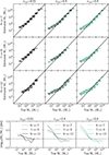 |
Fig. A.1. Upper Panel: estimated stellar mass, when adding 10% error to best fit and ruining CIGALE (mock test), as function of the True stellar mass from the σrun = 0.01, 0.4, and 0.8 for the different redshift bins. Lower Panel: ΔM★ = log(Estimated M★)−log(True M★) as function of the True stellar mass. |
We tested the impact of the rest-frame wavelength cover range on the estimation of M★ for galaxies in the last redshift bin. To account for this, we removed the longest NIRCam filters of the galaxies at 6 < z < 7 to mimic the rest-frame coverage of galaxies at z∼11. In Fig. A.2, we compare the stellar mass distribution estimated with CIGALE using all available filters (x-axis) and using only those covering wavelengths up to 0.4 μm (y-axis). In an ideal scenario, we would expect a perfect match (ΔM★ = 0), meaning that the rest-frame wavelength range (within JADES filters) does not affect the stellar mass estimation. However, as seen in Fig. A.1, some level of uncertainty persists because we do not cover ≳1 μm rest-frame. In the worst case, the impact of the rest-frame wavelength coverage (within our sample) would add to the uncertainty introduced by the absence of mid-infrared constraints. For all SFH models, the stellar masses are generally well-recovered. The mass-dependent trend is observed, with a mild overestimation that flattens around ∼0.2 dex at ∼108 − 109 M⊙. At the high-mass end of the stellar mass range (≳1010 M⊙), the M★ is underestimated by ∼0.1 dex for σrun > 0.1, though this trend is driven by a small number of sources.
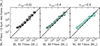 |
Fig. A.2. Stellar mass derived from filters up to 0.4 μm rest-frame as a function of the stellar mass derived from all filters, for galaxies at 6 < z < 7 for σrun = 0.01, 0.4, and 0.8. |
It is well known that the overestimation of M★ in the absence of rest-frame NIR constraint is primarily driven by the age-attenuation degeneracy and contamination from emission lines. Without restframe near/mid-infrared constraints, the SED fitting tends to favor younger stellar populations with higher attenuation, leading to overestimated M★ (Papovich et al. 2023; Williams et al. 2024; Cochrane et al. 2025; Wang et al. 2025b).
Appendix B: Physical properties of the sample
We present the evolution of the physical properties of our classified sample (see Sect. 5) in Fig. B.1. In this figure, we show the normalized distributions of UV magnitude, SFR, stellar mass, and UV slope for both galaxies with bursty and smooth SFH. The median MUV of bursty galaxies is brighter by 1.26 and 1.15 mag compared to those with smooth SFHs at 6 < z < 7 and 7 < z < 9, respectively, while it is ∼0.25 mag fainter at z > 9. A similar trend is observed in the SFR distributions: bursty galaxies exhibit SFRs higher by ∼1 dex at z < 9, but lower by ∼0.4 dex at z > 9. Nevertheless, they also reach the lowest SFR values in the sample. The UV slope (β) shows a similar trend, with bursty galaxies being ∼0.2 bluer at z < 9 and ∼0.4 redder at z > 9. The median stellar mass shows small differences, although at z < 9 bursty galaxies are ∼0.5 dex more massive.
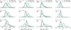 |
Fig. B.1. Normalized distributions of the physical properties of classified galaxies as stochastic (light green) and τ−delayed (dark green) at 6 < z < 12 in our sample. From left to right: UV magnitude, star formation rate, stellar mass and UV β slope. |
Appendix C: Validation of SFH Classification with Bayes factor
C.1. Impact of the S/N on the Classification
To provide a purity estimate of our classified sample and test the impact of the S/N on the classification from the Bayes factor (see Sect. 5.1), we used the best-fit models of the CIGALE run of the JADES galaxies as simulated observations to evaluate the fraction of misclassified galaxies in each category. From this set of SEDs, we know all the properties. This simulation provides a more realistic set of data than the mock catalogs presented in Sect. 2.2, which were built from a flat grid of parameters.
For each of these SEDs, we choose either the one obtained from the fit with σrun = 0.01 or from the fit with σrun = 0.8. We thus constitute a sample of galaxies that are labeled either as “smooth” or “bursty”. We do a new CIGALE run on this simulated sample and apply our classification to test it, especially the impact of the S/N on it. In Table C.1, we provide the results of this test for several S/N bins, from 0-5 to 20-30, and for two BF thresholds. The fraction of bursty galaxies classified as bursty (true positive) increases with the S/N for both BF thresholds, and thus the fraction of bursty galaxies classified as smooth (False negative) decreases. With a BF threshold of 3, as used in our analysis, the fraction of bursty galaxies classified as such varies from 35% to 88% depending on the S/N. Hence, we are missing bursty galaxies, especially at low S/N (typically low-mass galaxies), but using this threshold, our sample is pure with only 5% contamination from smooth galaxies wrongly classified as bursty. Our selection of bursty galaxies is thus quite conservative.
Validation of SFH Classification with Bayes factor for realistic simulated observations with bursty and smooth SFHs as a function of S/N.
C.2. Performance Test
To evaluate the robustness of our classification method based on the Bayes factor (see Sect. 5.1), we carried out controlled experiments using the mock catalogs built in Sect. 2.2, with the input parameters listed in Table 1. To reproduce realistic conditions, we added realistic noise, ensuring that the flux uncertainties follow the same distribution as in the observations. These simulated catalogs allow us to quantify possible biases in the recovered fractions and the reliability of the classification method.
In the mock catalogs we have a set of simulated observations with a given SFH model (σmock = 0.01, 0.8). We use CIGALE to fit each mock catalogs using different values of σrun = 0.01, 0.8, as for the observations (see Sect. 2.2 for details). Then, we applied the classification method using BF, to evaluate the impact on the derived “burst” and “smooth” fraction. Galaxies with BF> 3 are classified as bursty (stochastic), while those with BF≤3 are considered smooth. Therefore, in a given redshift or mass bin, the fraction of bursty systems corresponds to the number of galaxies with BF> 3 divided by the total number of galaxies.
First, we applied this classification to each individual mock catalog. In an ideal case, the recovered bursty fraction should be zero for the smooth catalog (σmock = 0.01) and unity for the bursty one (σmock = 0.8). The fraction of smooth galaxies misclassified as bursty remains below 15% at all redshifts, meaning that the fraction of true smooth systems correctly classified is ∼85%. Conversely, around 50% of galaxies in the bursty catalog are correctly identified as bursty. This implies that we are underestimating the number of stochastic systems, rather than overestimating them, given the low contamination fraction from smooth galaxies.
Then, we built mock, observationally based, catalogs with different intrinsic fractions of bursty galaxies (30%, 50%, and 70%) and applied the same classification approach. For the catalog with the lowest intrinsic bursty fraction (30%), the contamination fraction of smooth galaxies is ∼8%. Although this contamination appears relatively high, it is mainly driven by the large number of smooth systems in this sample, which statistically increases the number of false positives. In contrast, when stochasticity dominates (70%), the contamination falls to only ∼4%. In this case, the purity of the smooth classification is high (around 90%), and the underestimation of the bursty fraction becomes the main effect. In the intermediate case, with an intrinsic bursty fraction of 50%, the contamination remains below < 6%.
In these tests, the computed fractions do not evolve significantly with redshift, indicating that no systematic bias is introduced that could mimic a decrease in the bursty fraction toward lower redshifts.
All Tables
CIGALE input parameters used to build the mocks SEDs and to fit the spectrum of galaxies at z ≥ 6.
Spearman correlation coefficients for the SFR10 − M* plane with the different SFH models (σrun) in the three redshift bins.
Properties derived from SED modeling of the mass-complete sample assuming σrun = 0.01, 0.4, and 0.8.
Validation of SFH Classification with Bayes factor for realistic simulated observations with bursty and smooth SFHs as a function of S/N.
All Figures
|
Fig. 1. Stochastic star formation histories (SFRsmooth × SFRstochastic) for different combinations of parameters generated with the STOCHASTICSFH module. Each panel shows the impact on the SFH of one specific parameter: σ (left panel), τbreak (middle panel), and α (right panel), in all cases the age and τmain are fix to 500 and 1000 Myr, respectively. |
| In the text | |
|
Fig. 2. Color-color diagram using JWST/NIRCam bands from the JADES catalog (left columns) and from the simulated catalogs (from second to last columns). These simulated catalogs are computed assuming, from left to right, σ of 0.01, 0.1, 0.4, and 0.8. The two different rows show the color-color diagram obtained with two different band combinations chosen to take into account redshift and parameter coverage to ease the comparison. The color lines show the contours that enclose the 16th, 50th, 84th, and 90th of the data in the observations. The implemented stochastic SFH can reproduce observed colors at z > 6. |
| In the text | |
|
Fig. 3. χ2 obtained by fitting the mock catalogs with CIGALE. The different fits for each simulated catalog are color-coded by σrun used in the fit. A high level of burstiness (σrun ∼ 0.8) provides good fit quality, whatever the intrinsic level of burstiness of the fitted galaxy, while smoother SFHs struggle to fit bursty galaxy SEDs. |
| In the text | |
|
Fig. 4. Comparison between the mock SFR10 (true SFR10) and the SFR10 recovered by CIGALE (estimated SFR10) for all mock catalogs (rows) fitted with the different values of σrun (columns). The boxes span from the first quartile (Q1 = 25%) to the third quartile (Q3 = 75%), with a line indicating the median position, while the error bars extend from the 16th to the 84th percentile of the cumulative distribution. The gray background in the panels highlights when σrun match σmock. The SFH with the highest level of burstiness (σrun = 0.8) provides the best estimate of SFR10. |
| In the text | |
|
Fig. 5. χ2 distribution of the whole sample for each CIGALE run. The σrun used to model the SFH is indicated by the x-axis. The black dashed line shows the median χ2 for σrun = 0.8. The embedded box plot of each distribution indicates the median, interquartile range (IQR), and whiskers. A high level of burstiness accounted for in the SFH is needed to fit early galaxies’ SED. |
| In the text | |
|
Fig. 6. Example SED of a galaxy at z ∼ 6 (top panel) and residuals (bottom panel). The dark purple squares are the fluxes from HST and JWST. The solid lines are the best-fit models obtained by CIGALE. The open circles indicate the modeled fluxes for the different models (in the top panels only for σrun = 0.8). |
| In the text | |
|
Fig. 7. SFR–M★ relation obtained from different burstiness levels in the SFH, color-coded by the assumed σrun. The dashed and dotted gray lines show when the classified sample (see Sect. 5) is 85% and 95% complete, respectively. The blue line shows the SFR–M★ from Popesso et al. (2023), converted from a Kroupa & Boily (2002) to a Chabrier (2003) IMF. The scatter of the MS strongly depends on the burstiness encoded in the assumed SFH. |
| In the text | |
|
Fig. 8. Fraction of high-mass (8.8 < log M★/M⊙ < 9.5) galaxies classified as bursty as a function of redshift using the Bayes factor (see Sect. 5.1). The left panel shows the results when full spectral information at each redshift is used, while the right panel shows the results assuming the same rest-frame wavelength coverage as a galaxy at z = 11. Uncertainties on the fractions are derived from Poisson distribution, while uncertainties on the redshifts correspond to the 16th–84th percentile range of the redshift distribution within each stellar mass bin. The gray downside triangles show the fraction of stochastic massive galaxies (log M★ > 9) found in Ciesla et al. (2024), obtained from the variations of the recent SFR using nonparametric SFH. There is a trend showing an increasing fraction of bursty galaxies with increasing redshift that is not due to the difference in wavelength coverage. |
| In the text | |
|
Fig. 9. Evolution of the log10(SFR10/SFR100) ratio, used as an indicator of burstiness, as a function of redshift. Blue contours indicate the distribution of the galaxies of our sample classified as having a bursty SFH. The big square and diamonds indicate the median value for each of the three redshift bins considered in this work for bursty galaxies with enhanced SF activity and decreasing activity, respectively. The black solid line is a linear fit to the ratio obtained for galaxies classified as having a smooth SFH. Measurements from the literature are also shown for comparison (Cole et al. 2025; Kokorev et al. 2025; Carniani et al. 2024). The SFR10/SFR100 ratio from Arrabal Haro et al. (2023), Castellano et al. (2024), Hsiao et al. (2024), Bunker et al. (2023), Álvarez-Márquez et al. (2025), Fujimoto et al. (2024), Napolitano et al. (2025) were taken from Kokorev et al. (2025). The light blue shaded regions represent the log10(SFR10/SFR100) distribution within 1-σ for bright galaxies (MUV < −20; Kokorev et al. 2025) and the 16th–84th percentiles from Cole et al. (2025), with the median indicated by the solid line. The right panel shows the distribution of log10(SFR10/SFR100) ratios obtained from the simulated mock catalogs with different burstiness levels presented in Sect. 2.2. The ratio is constant as a function of redshift. Only high ratios of ≳0.2 cannot be reproduced by a smooth SFH. |
| In the text | |
|
Fig. 10. Evolution of σUV with the redshift for our sample in JADES at 6 < z < 12. The uncertainties on σUV are estimated from bootstrapping. The error bar on redshifts indicates the 16th to 84th percentiles of the distributions. The blue shades and markers show estimations from the literature, which are based on semi-analytical models and simulations (Pallottini & Ferrara 2023; Shen et al. 2023; Muñoz et al. 2023; Mason et al. 2023) or observations (Ciesla et al. 2024; Shuntov et al. 2025a). Our estimate σUV is consistent with the literature and too low to explain the mild evolution of the UVLF at z > 10 only from bursty SFH, as estimated by Shen et al. (2023) (empty circles) using empirical models. |
| In the text | |
|
Fig. 11. Instantaneous star formation efficiency as a function of halo mass for the three redshift bins in our sample. Solid lines and shaded regions show the estimates from Shuntov et al. (2025a), based on the UV luminosity function and halo occupation distribution (HOD) modeling. Our estimates of ϵ do not show any strong variation with redshift and confirm the low values obtained by Shuntov et al. (2025a). |
| In the text | |
|
Fig. A.1. Upper Panel: estimated stellar mass, when adding 10% error to best fit and ruining CIGALE (mock test), as function of the True stellar mass from the σrun = 0.01, 0.4, and 0.8 for the different redshift bins. Lower Panel: ΔM★ = log(Estimated M★)−log(True M★) as function of the True stellar mass. |
| In the text | |
|
Fig. A.2. Stellar mass derived from filters up to 0.4 μm rest-frame as a function of the stellar mass derived from all filters, for galaxies at 6 < z < 7 for σrun = 0.01, 0.4, and 0.8. |
| In the text | |
|
Fig. B.1. Normalized distributions of the physical properties of classified galaxies as stochastic (light green) and τ−delayed (dark green) at 6 < z < 12 in our sample. From left to right: UV magnitude, star formation rate, stellar mass and UV β slope. |
| In the text | |
Current usage metrics show cumulative count of Article Views (full-text article views including HTML views, PDF and ePub downloads, according to the available data) and Abstracts Views on Vision4Press platform.
Data correspond to usage on the plateform after 2015. The current usage metrics is available 48-96 hours after online publication and is updated daily on week days.
Initial download of the metrics may take a while.