| Issue |
A&A
Volume 704, December 2025
|
|
|---|---|---|
| Article Number | A137 | |
| Number of page(s) | 18 | |
| Section | Extragalactic astronomy | |
| DOI | https://doi.org/10.1051/0004-6361/202556621 | |
| Published online | 05 December 2025 | |
Wide-Field uGMRT band-3 Imaging of the Fields Around X-Shaped radio galaxies
Spectral properties of 4C32.25 and 4C61.23
1
Astrophysics Research Centre, School of Mathematics, Statistics and Computer Science, University of KwaZulu-Natal, Durban 4041, South Africa
2
Wits Centre for Astrophysics, School of Physics, University of the Witwatersrand, Private Bag 3, Johannesburg 2050, South Africa
⋆ Corresponding author: This email address is being protected from spambots. You need JavaScript enabled to view it.
Received:
28
July
2025
Accepted:
26
September
2025
Abstract
We present wide-field upgraded Giant Metrewave Radio Telescope (uGMRT) images of the fields around the X-shaped radio galaxies (XRGs) 4C32.25, 4C61.23, and MRC 2011–298 obtained at 400 MHz. The observations are calibrated using the extreme peeling method to account for direction-dependent effects across the field of view, as was previously applied to Low-Frequency ARray (LOFAR) data. Our 400 MHz images capture in fine detail the radio morphology of the XRGs, as well as other serendipitous radio sources located in these fields. We use these images along with archival low-frequency and high-frequency radio data to investigate the spectral properties of the XRGs 4C32.25 and 4C61.23. Under the assumption of conditions corresponding to the maximum radio source age, we estimate the spectral ages of both the primary lobes and the wings. These ages indicate that the wings are the oldest component of the XRGs and are a product of past radio activity. Moreover, we have used the radio images available to derive high-resolution spectral index maps for these two XRGs. We find that the spectral index steepens from the primary lobes toward the wings, consistent with our spectral age estimates. These results suggest that precessional and backflow models explain the X-shaped radio morphology of 4C32.25 and 4C61.23, respectively. Finally, taking advantage of our wide-area images, we identify several serendipitous diffuse radio sources located in our XRG fields and cross-reference them with previous surveys.
Key words: galaxies: active / galaxies: evolution / galaxies: formation / galaxies: jets / galaxies: nuclei
© The Authors 2025
 Open Access article, published by EDP Sciences, under the terms of the Creative Commons Attribution License (https://creativecommons.org/licenses/by/4.0), which permits unrestricted use, distribution, and reproduction in any medium, provided the original work is properly cited.
This article is published in open access under the Subscribe to Open model. This email address is being protected from spambots. You need JavaScript enabled to view it. to support open access publication.
1. Introduction
The observed scaling relations between the masses of supermassive black holes (SMBHs) and those of their host galaxies suggest a clear link between the growth of both components (e.g., Magorrian et al. 1998; Ferrarese & Merritt 2000; Kormendy & Ho 2013). The growth of a SMBH occurs via mergers and episodes of gas accretion. During the accretion or active phase, known as active galactic nucleus (AGN), the SMBH releases vast amounts of energy in the form of electromagnetic radiation, relativistic plasma jets, and high-speed gas outflows (Alexander et al. 2025). With modern radio-interferometers it is possible to observe with detail the extended radio morphologies of low-z radio galaxies hosting SMBHs (Morris et al. 2022; Xie et al. 2024; Clews et al. 2025). These morphologies are usually divided into two categories: Fanaroff-Riley type I (FRI) sources, which are characterized by dimmed edges exhibiting bending jets and radio emission that peaks near the core, and edge-brightened Fanaroff-Riley type II (FRII) sources, which feature well-collimated jets, an expansive pair of radio lobes, and prominent hotspots (Fanaroff & Riley 1974). A sub-class of radio galaxies is characterized by the presence of two pairs of radio lobes associated with a single host galaxy. These galaxies are called X-shaped radio galaxies (XRGs) due to the two radio-lobe pairs having high average alignment angles of ∼70° (e.g., Capetti et al. 2002; Bruno et al. 2019; Joshi et al. 2019), which give rise to their distinctive X-shaped morphology. The primary lobe pair (i.e., the active one) usually shows hot spots, whereas the secondary lobe pair (i.e., wings) has lengths shorter or comparable to those of the primary pair (Leahy & Williams 1984; Capetti et al. 2002; Joshi et al. 2019), and is often devoid of hot spots. The majority of XRGs can be classified as FRII, while the rest are either FRI or presenting a FRI and FRII hybrid morphology (Merritt & Ekers 2002).
Several theoretical models have been proposed in the literature to explain the origins of XRGs (see Gopal-Krishna & Chitre 1983; Gopal-Krishna et al. 2012 or Giri et al. 2024 for a review). The main formation models differ significantly: in the backflow model, the wings are formed as a result of the deflection of plasma coming from the terminal hotspots due to buoyancy forces upon impinging on the host thermal halo (Leahy & Williams 1984) or due to a pressure gradient between the host axes (Capetti et al. 2002); while in the reorientation models the wings are fossil emission from previous jets that undergo a slow axis precession (Rees 1978; Parma et al. 1985), or may experience an abrupt change in their direction (“spin-flip”) due to a minor merger event (Dennett-Thorpe et al. 2002; Merritt & Ekers 2002). Other models from the literature include the jet-shell model that predicts that a merger with a gas-rich disk galaxy activates the SMBH and creates a series of stellar shells (Oke & Gunn 1983; Gopal-Krishna et al. 2012). The wings are the result of the jet disruption by the stellar shells. Another model is the dual-AGN system, in which the radio lobes and wings are fueled by an unresolved dual-AGN system at the core of the host galaxy (Lal & Rao 2007; Lal et al. 2019). In this model, both AGNs are active at the same time, thus, there should not be systematic differences in the spectral indices of the radio lobes and wings. This goes against the expectations of the other models, as the wings are expected to be filled with older radio emission than the primary lobes and hence the wings should not present a radio spectrum statistically indistinguishable from that of the primary lobes. Evidence against the dual-AGN models was found by Patra et al. (2023), who using a wide frequency range (150−1400 MHz) found that their XRG sample presents a rich variety of spectral features, in contrast with the results of the XRG sample by Lal et al. (2019), in which the lobes and wings show similar spectral properties using a narrower frequency range (240−610 MHz). However, Yang et al. (2022) provided evidence of a XRG associated with a dual-AGN system using 5 GHz VLBI observations.
Over the past two decades, the advent of large-area radio-sky surveys such as FIRST (Becker et al. 1995), NVSS (Condon et al. 1998), TGSS (Intema et al. 2017), and LoTSS (Shimwell et al. 2017, 2022) has significantly increased the number of known XRGs since their designation as a new radio source class by Leahy & Parma (1992). For instance, Cheung (2007) compiled a total of 100 XRG candidates in the FIRST survey, doubling the number of XRGs at the time. Later, Proctor (2011), using an automated pattern recognition method, identified 134 new XRG candidates using FIRST data. Yang et al. (2019) presented a new catalog of 265 XRG candidates by combining FIRST and TGSS data. More recently, Bhukta et al. (2022) and Bera et al. (2022) discovered about 40 and 14 new XRG candidates using TGSS and LoTSS DR1 radio maps, respectively.
Low-radio frequency observations (< 1 GHz) provide unique data that may help to resolve some questions related to the link between AGNs and their radio morphologies (e.g., Lal et al. 2019; Brienza et al. 2020; Bera et al. 2022), and the mechanisms triggering SMBH activity (e.g., Sabater et al. 2019; Retana-Montenegro & Röttgering 2020; Retana-Montenegro 2022). However, such observations have been limited by direction-dependent effects (DDEs) such as the ionospheric corruption of the visibility data, imperfect knowledge of the antenna beams, and strong radio-frequency interference. Therefore, it is of paramount importance to account for DDEs to obtain deep high-fidelity images at low radio frequencies. Different calibration strategies have been used to correct DDEs for different radio telescopes: GMRT (Intema et al. 2009, 2017), LOFAR (van Weeren et al. 2016; Williams et al. 2016; Retana-Montenegro et al. 2018; Tasse et al. 2021), and MeerKAT (Tasse 2014; Tasse et al. 2018). In this work, we use a modified implementation of the extreme-peeling technique used by Retana-Montenegro et al. (2018) (hereafter, RM18) in the NDWFS-Boötes field to calibrate upgraded GMRT (uGMRT, Gupta et al. 2017) 250−500 MHz band-3 observations of three XRGs fields (4C32.25, 4C61.23, and MRC 2011–298). These observations provide a testbed for our uGMRT direction-dependent calibration strategy, which allows us to obtain deep high-fidelity images.
The main purpose of studying XRGs fields is threefold. Firstly, to understand the physical mechanisms that lead to their distinct X-shaped morphology. The radio galaxies 4C32.25 (Parma et al. 1985; Gregorini et al. 1992a; Mack et al. 1994; Klein et al. 1995; Rengelink et al. 1997; Condon et al. 1998; Cohen et al. 2007) and 4C61.23 (Condon et al. 1998; Lara et al. 2001a; Cohen et al. 2007) offer an excellent opportunity to probe the formation mechanisms of XRGs. The higher sensitivity and angular resolution of uGMRT band-3 allows us to study in great detail the spectral properties of these two XRGs at low-frequencies. Secondly, to investigate in detail the entire fields surrounding these XRGs, searching for diffuse sources or AGNs serendipitously located within them. Previously, analyses of the same data focused only on the central XRGs (Sebastian et al. 2024; Bruno et al. 2024), while we calibrate, image, and analyze the entire fields. Thirdly, to demonstrate the robustness of our uGMRT direction-dependent calibration strategy.
This paper is organized as follows. In Section 2, we describe the XRGs analyzed in this work. A summary of the datasets used is presented in Section 3. In Section 4, we introduce our calibration method based on the extreme peeling technique. Section 5 discuss our mosaics and source catalogs. Section 6.1 presents our results. These include our wide-field uGMRT images, integrated synchrotron spectra, spectral ages, and spectral-index maps of 4C32.25 and 4C61.23. In Section 6.3, we present a sample of serendipitous radio sources located in our XRGs fields. Finally, we provide our summary and conclusions in Section 7. Throughout this paper, we use a Λ cosmology with the matter density Ωm = 0.30, the cosmological constant, ΩΛ = 0.70, the Hubble constant, H0 = 70 km s−1 Mpc−1. We assume a definition of the form Sν ∝ να, where Sν is the source flux density, ν the observing frequency, and α the spectral index.
2. Targets
2.1. Radio galaxy 4C32.25 (B2 0828+32)
The radio galaxy 4C32.25 (also known as B2 0828+32) presents prominent wings that are over a factor of two more extended than its radio lobes (e.g., Rengelink et al. 1997; Condon et al. 1998). The luminosity profiles of the host galaxy show weak signatures of a recent merger event (Ulrich & Roennback 1996). The radio galaxy has a total flux density of S1.4 GHz = 1.8 Jy (Condon et al. 1998), and a redshift of zspec = 0.0507 (Landt et al. 2010). While its radio lobes indicate an FRII type morphology, the radio-luminosity, L178 MHz = 2.60 × 1024 W Hz−1, is approximately one order of magnitude below the FRI and FRII threshold (1 × 1025 W Hz−1, at 178 MHz; Fanaroff & Riley 1974). The source presents high fractional levels of polarization in the lobes and wings (Parma et al. 1985; Gregorini et al. 1992a; Mack et al. 1994; Rottmann 2001). Previous spectral studies found that at frequencies higher than 1.4 GHz there is a progressive steepening of the spectral index along the wings, with values of α ∼ −0.6 in the radio lobes to steeper values of α ∼ −1.2 in the wings (Klein et al. 1995; Rottmann 2001). In contrast, low-resolution observations at 325−609 MHz show that the spectral index is relatively flat along the wings with values of α ∼ −0.6 (Rottmann 2001).
2.2. Radio galaxy 4C61.23
4C61.23 is associated with a spheroidal galaxy with strong emission lines (Lara et al. 2001b). The radio galaxy has a total flux density of S1.4 GHz = 1.18 Jy, and a redshift of zspec = 0.111 (Lara et al. 2001a). Morphologically, 4C61.23 is a symmetric FRII type source, whereas the radio-luminosity, L178 MHz = 8.55 × 1024 W Hz−1. This radio-luminosity is just below the FRI and FRII division. Additionally, there are strong indications that suggest a backflow emanating from both radio lobes, which is redirected in opposite directions perpendicular to the jet axes (Condon et al. 1998; Lara et al. 2001a). There is evidence from high-resolution VLBA images that show that 4C61.23 may be a binary black hole candidate (Liu et al. 2018; Sebastian et al. 2024). Finally, the spectral study by Sebastian et al. (2024) found that the jets exhibit steeper spectra than the wings.
2.3. Radio galaxy MRC 2011–298
MRC 2011–298 (zspec = 0.1366, Jones et al. 2009) is the brightest cluster galaxy (BCG) of the galaxy cluster A3670, a richness-class 2 galaxy cluster (Coziol et al. 2009). This BCG is a giant elliptical galaxy with an ellipticity of ϵ = 0.14 (Makarov et al. 2014) and is classified as a dumbbell galaxy due to the presence of two bright optical cores surrounded by a stellar halo (Andreon et al. 1992; Gregorini et al. 1992b). MRC 2011–298 was first classified as an XRG candidate by Gregorini et al. (1994), and confirmed later by Bruno et al. (2019). The XRG presents a pair of north-south lobes with a pair of weak wings oriented almost perpendicularly to the lobes. Recently, Bruno et al. (2024) found that the S-shaped morphology of the jets makes precession a strong explanation for the jet bending. They also show that spin-flip is the likely formation process for the overall X-shaped structure. These authors also found that the wings are fainter than the lobes at all frequencies. The radio galaxy has a flux density of S1.4 GHz = 407.3 mJy (Condon et al. 1998), and a radio-luminosity of L178 MHz = 2.60 × 1024 W Hz−1.
3. Data
In this section, we present the observations of the XRGs and describe the archival radio-data employed in this work. The details of the radio data are summarized in Table 1.
Summary of the uGMRT band-3 observations.
3.1. uGMRT band-3 data
The XRGs 4C32.25, 4C61.23, and MRC 2011–298 were observed with the uGMRT wide-band receiver (GMRT Wideband Backend, GWB, Gupta et al. 2017) in band 3 (250−500 MHz) for 2.8, 3, and 8 hours, respectively. The observations include 10-minute pointings on 3C147 and 3C48, which were used as flux density calibrators. The calibration process is described in Section 4.
3.2. LoTSS data
The LOw-Frequency ARray (LOFAR) Two-metre Sky Survey (LoTSS; Shimwell et al. 2017, 2022) is an ongoing LOFAR survey of the northern sky at 144 MHz. The LoTSS images have a median noise level of 83 μJy/beam with a resolution of ∼6″. The fields of 4C32.25 and 4C61.23 are both covered by LoTSS. We use the high-resolution LoTSS images available from the LoTSS archive1.
3.3. VLA data
First, we browsed the NRAO VLA Archive Survey (NVAS2; Crossley et al. 2008) looking for archival images of our XRGs. The NVAS provides access to VLA images from 1976 to 2006 processed using the AIPS pipeline Greisen (2003). We find that 4C32.25 and 4C61.23 have images available at 1.5 GHz and 4.89 GHz, respectively. The angular resolutions and noise levels of these images are 13″, 5″ and 0.483 mJy/beam, 0.167 mJy/beam, respectively. We complement these data with images from the NVSS (Condon et al. 1998), FIRST (Becker et al. 1995), and VLASS (Lacy et al. 2020) surveys at 1.4 and 3.0 GHz, respectively. The angular resolutions and typical noise levels of these surveys are 5″, 45″, 2.5″; and 0.15 mJy/beam, 0.45 mJy/beam, 120 μJy/beam, respectively. Finally, for 4C32.25, we also analyze archival S-Band data (ID: VLA/22B-144) from the NRAO archive3. The observations were performed on January 1st, 2023. The target was observed in a single scan for a total integration time of 0.56 hours. Observations were carried out with the VLA in C configuration. The source 3C147 was used as flux density calibrator. The sampling time was set to 5 s and four polarization products (RR, LL, RL, and LR) were obtained. The total bandwidth, equal to 2 GHz in the range 2−4 GHz, was divided into 16 sub-bands of 128 MHz with 64 frequency channels. We used the Common Astronomy Software Applications (CASA, McMullin et al. 2007) to perform a standard calibration4 of the VLA dataset. The final image of the target is 0.64° ×0.64° in size and was made using WSClean (Offringa et al. 2014), where we impose an inner uv-limit of 50λ, and Briggs (1995) Brigg’s weighting with a robustness parameter of 0. The image has a resolution of ∼5″ and central noise of 14 μJy/beam.
3.4. RACS data
The Rapid ASKAP Continuum Survey (RACS) is a large-area survey with the full 36-dish ASKAP radio telescope. RACS aims to image the entire sky (south of Dec 51°) at 887.5 MHz (RACS-low), 1296 MHz (RACS-mid), and 1656 MHz (RACS-high), with a bandwidth of 288 MHz (McConnell et al. 2020; Hale et al. 2021; Duchesne et al. 2023, 2025). RACS-low has an angular resolution of 15″ with an average noise level of 0.25 mJy/beam, RACS-mid has a resolution of 10.2″ and median noise of 182 μJy/beam, and RACS-High maps have a resolution of 9.78″ and median noise of 195 μJy/beam. The fields of 4C32.25 and MRC 2011–298 are covered by RACS-low and RACS-mid. For these two fields, we retrieve the RACS images from the CASDA archive5.
4. uGMRT data processing
To process the uGMRT data, we used the extreme-peeling calibration technique used by RM18 to calibrate LOFAR data of the NDWFS-Boötes field. The direction-independent and direction-dependent stages are described in the following sections.
4.1. Direction-independent calibration
First, we retrieved the raw data from the uGMRT Online archive6. The raw visibilities in UVFITS format were converted to the Measurement Set (MS) format7 using the CASA routine importgmrt8. The MS files were later converted to a LOFAR-compatible format (Offringa et al. 2013). These MS files are regularly shaped, meaning that all the time slots have the same baselines and channels contained within a single spectral window. The primary flux density calibrator and target scans were separated from the original MS file with the CASA task split. The unaveraged scans were flagged to remove radio frequency interference (RFI) using a custom LUA AOflagger script (Offringa et al. 2010, 2012). The flagging includes the bandpass edges, and the high-RFI frequency ranges 360−379.6 MHz and 486−500 MHz, which generally present poor signal-to-noise (S/N). After flagging, the data were averaged to a resolution of 512 channels per scan from the original resolution of 2048 channels. The data were not averaged in the time axis to capture the rapid changes in the ionospheric conditions.
The first stage involved using the primary flux density scan in three steps. The first step was obtaining the XX and YY gain solution toward the flux density calibrator using the LOFAR skymodel. The primary flux density calibrator of each field is indicated in Table 1. This skymodel was normalized to the flux density scale of Scaife & Heald (2012) (hereafter SH12). The gains were computed using the open-source solver DP3 (van Diepen et al. 2018). The second step was to determine the clock offsets between the core and the (southern, western, and eastern) arms uGMRT antennas using the primary flux density calibrator phases solutions. The clock offsets for the 4C32.25 field are shown in Figure 1. The largest negative between core and arms is close to 120 ns. The other two fields have similar bimodal distributions in their clock offset values: for 4C61.23, the maximum offset is about 100 ns, while the offsets for MRC 2011–298 are smaller, with the largest offset being 30 ns. The third step is to measure the XX and YY phase offsets for the calibrator.
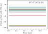 |
Fig. 1. Fit clock differences using the gain solutions from 3C147. The values show a bimodal distribution between core and arm antennas (mainly from the southern arm). The colors represent different antennas. |
For the second stage, a series of steps involving the target scan were performed to obtain the DI images of the target field. The flow diagram of the direction-independent calibration part is shown in Figure 2. Firstly, the target scans were created, averaged, and flagged using the same method as described for the calibrator scans. Secondly, DP3 was used to the transfer of amplitudes, clock values and XX–YY phase offsets from the flux density calibrator to the target. The gain amplitudes were filtered and smoothed to eliminate significant outliers. This flagged visibility data related to the eliminated gain outliers. Thirdly, with DP3 we performed three phase-only calibration cycles combining all the target scans using a beam-attenuated TGSS skymodel (Intema et al. 2017). We used the polynomial beam model described in the uGMRT users manual9 to attenuate the skymodel. Imaging was carried out using WSClean (Offringa et al. 2014), for which we imposed an inner uv-limit of 50λ, and a Briggs (1995) robust weighting parameter of 0. This value provides a compromise in weighting between the core and edge baselines. WSClean was run with multi-frequency deconvolution and multiscale modes enabled, in order to address the wide bandwidth of the data and to better recover the diffuse emission in the uGMRT maps. The total size of our images was 6500 × 6500 pixels with a pixel size of 2″. Fourthly, three additional amplitude-phase calibration cycles were performed using the skymodel obtained in the last step.
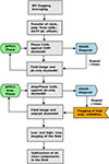 |
Fig. 2. Schematic view of the direction-independent calibration steps for uGMRT Band 3 data. |
Finally the skymodel from the last calibration cycle was used to subtract the high-resolution clean components from the visibilities. We imaged the new residual visibilities at low-resolution using a Gaussian taper of 10″ to account for any diffuse emission component resolved out at high-resolution. This low-resolution skymodel was subtracted from the high-resolution subtracted visibilities to obtain new residual DI visibilites with both low- and high-resolution CLEAN components subtracted to obtain DI residual visibilities. This subtraction will be improved iteratively during the directional self-calibration process. Finally, the low-resolution model was combined with the high-resolution one to obtain the complete DI skymodel of the target field.
4.2. Direction-dependent calibration
Artifacts caused by direction-dependent (DD) effects, as antenna-antenna beam variations and ionospheric distortions were still present in our DI images. Schwab (1984) suggested that as long DD effects vary slowly accross the field of view (FOV) it is possible to discretize it into smaller regions or facets. For each facet, a self-calibration process can be done to correct the visibilities for DD effects. This can be repeated until the facets in the FOV are corrected. A critical part in the FOV discretization, is that each facet must have a bright source or a group of closely spaced bright sources in order for the self-calibration process to converge. The resulting facet images are used to improve the DI residual visibilities. Based on our experience, sources brighter than 0.1 Jy were good facet calibrators. The facet distribution for our three fields are shown in Figure 4. The facet calibrators varied from field to field, with nine facets for the 4C61.23 field, while the MRC 2011–298 field required only three facets.
The flow diagram of the direction-independent (DD) calibration part is shown in Figure 3. The first step was to shift the DI residual visibilities to the direction of the facet calibrator, adding it back to the UV data. In the first and second cycles, we solved for scalar Jones phase offsets and total ionospheric electron content (TEC) terms on short timescales (fast gains), which cause frequency-dependent ionospheric distortion on the phases. In subsequent cycles, we began by solving for scalar phase+TEC only followed by the diagonal Jones phase+amplitude solutions over longer timescales to capture the slower variations in the beam (slow gains). The solution intervals used for fast gains are 4 channels and 1 time step; while for slow gains, they were 30 channels and 100 time steps. The self-calibration cycle could be repeated until artifacts around bright facet calibrators are reduced significantly and convergence is achieved. When the DD self-calibration cycle was completed, the DI residual visibilities were shifted to the direction of the facet center. The facet skymodel subtracted at the end of DI calibration was added back and the DD gain solutions were applied. The new facet skymodel was subtracted from the DI residual visibilities. By doing this, we ensured that the effect of the presence of bright calibrators was reduced and improves the subsequent subtraction of fainter facets. This process was done in descending order according to the facet calibrator flux density. Figure 5 displays the DD self-calibration sequence for various facet calibrators from the three different fields.
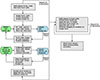 |
Fig. 3. Schematic view of the direction-dependent calibration steps for uGMRT Band 3 data. |
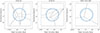 |
Fig. 4. The spatial distribution of facets in the 4C61.23, 4C25.25, and MRC 2011–298 fields. The blue circle denotes angular distance where the uGMRT beam is 50% of that at the pointing center; that is, about 0.74°. |
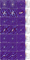 |
Fig. 5. Images showing a direction-dependent self-calibration sequence for facet calibrators from the different fields. The corresponding field name is indicated in the images of the first column. The first column displays the images made with only the DI self-calibration solutions. The central column displays the improvements after two iterations of fast phase (TEC and phase-offset)-only DDE calibration. The right-hand column shows the improvement after two further iterations of fast phase (TEC+phase offset) and slow phase and amplitude (XX and YY gain) DDE calibration. The scale is the same for all images of the self-calibration sequence. |
A relevant aspect to consider in uGMRT wide-field imaging is the mitigation of artifacts. For instance, amplitude artifacts usually manifests as ripples across the image background. We employed the UV plane outlier flagging approach by Sekhar & Athreya (2018) to eliminate ripples in our images. The principle behind this approach is that the ripples can be pinpointed as localized high-amplitude features in the UV plane using the residual (model – corrected) visibilities. These features are identified in annular regions in the UV plane. To prevent over-flagging due to the higher visibility density towards the center of the UV plane, we calculate a threshold for each annulus that is used to flag all outliers within the respective annulus. This method was used for the final facet imaging, and it was optional in each DD self-calibration cycle if it was needed to eliminate persistent ripples.
The final facets were imaged using the improved residual visibilities at full resolution, and were stitched together using casacore10. The primary-beam correction was applied using the same model used in Section 4.1. A radial-cutoff was imposed, where the uGMRT beam is 50% of that at the pointing center, which corresponds to a radius of ∼0.74°.
5. Images and source catalog
The final mosaics are shown in Figure 6. Table 2 summarizes the central root mean square (RMS) noise, angular resolution, and position angle for each mosaic.
Summary of the mosaics for the three fields considered.
We employed the Python Blob Detection and Source Finder (PyBDSM, Mohan & Rafferty 2015)11. package to create initial catalogs for the three fields. We used the pre-beam-corrected mosaics as the detection images, while the primary-beam corrected mosaics are the extraction images. The format of the three catalogs follows the same convections introduced in RM18.
The final catalogs of the fields 4C61.23, 4C32.25, and MRC 2011–298 contain a total of 799, 505, and 449 entries, respectively, detected above a 5σ flux density threshold. The astrometry and flux densities were corrected using the procedures described in RM18. Figure A.2 shows the flux density scale comparison between the uGMRT and the flux densities scaled to 400 MHz from the reference surveys LoTSS and RACS. Figure A.1 shows the corrected positional offsets. After we applied the corrections, the uGMRT astrometry and flux densities are in good agreement with those of FIRST and LoTSS/RACS, respectively. The catalogs are made available online12.
6. Results
6.1. Spectral properties
6.1.1. uGMRT images
The full-resolution 400 MHz uGMRT images of the XRGs are presented in Fig. 6. Our images confirm the X-shape morphology of the three radio galaxies, i.e. a pair of bright radio lobes and a pair of fainter wings. This is consistent with radio-maps from the same sources presented previously by other authors (Lal & Rao 2007; Bruno et al. 2019, 2024; Sebastian et al. 2024). The radio lobes are the brightest regions, while the core and wings are fainter. Each of the three XRGs exhibits a different orientation of its primary lobe axes. Both 4C32.25 and 4C61.23 are FRII sources due to the presence of hot spots in the jets, while MRC 2011–298 lacks hot spots in the jets making it a FRI source. The wings in 4C32.25 and MRC 2011–298 are significantly larger than their jets, which is rare (Saripalli & Subrahmanyan 2009; Joshi et al. 2019). The most striking feature is the large-scale wings of 4C32.25, which extend over ∼5′ (293 kpc) in length. The northern 4C32.25 wing is fainter than the southern wing, although it is approximately ∼11% longer. MRC 2011–298 has wings of similar length but displays asymmetrical morphologies with deflections at the edges, which along with the S shape of the jets could be related to jet precession (Bruno et al. 2024). The signature of deflections are weaker in 4C32.25, but it has been proposed that precession could explain its X-shaped morphology (Klein et al. 1995; Sebastian et al. 2024). The radio morphology of 4C61.23 is more symmetric with wings and jets of similar size and a faint radio core.
Our XRGs radio-maps demonstrate the robustness of our calibration approach to obtain high-fidelity, high-sensitivity images of diffuse radio emission. For instance, Bruno et al. (2024) analyzed the same dataset using the SPAM pipeline (Intema et al. 2009). In comparison, we not only do we improve the DD artifacts around the XRG, but also we also reach deeper noise levels at higher angular resolution (see Figs. 5 and 6). Compared to Bruno et al. (2024), our image exhibits improvements of about 45% in noise levels and 50% in angular resolution. A detailed comparison with SPAM is outside the scope of this work.
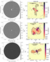 |
Fig. 6. Right: 400 MHz uGMRT mosaics of the 4C32.25, 4C61.23, and MRC 2011–298 fields. The area of each mosaic is approximately 1.72 deg2. The details of each field are summarized in Table 2. Left: Full-resolution uGMRT 400 MHz band-3 images of the three XRGs 4C32.25, 4C61.23, and MRC 2011–298. The contour levels are (1, 2, 4, 8, …)×3σ mJy/beam, where σ is the local noise level. The −3σ contours are denoted by dashed lines. The restoring beam is indicated by an ellipse in the bottom left corner. The black line indicates the corresponding angular scale. |
6.1.2. Integrated spectra and spectral aging
For each XRG, we combined all the flux densities available along with prior measurements from the literature to construct integrated synchrotron spectra. Particularly, LOFAR and uGMRT measurements trace the lowest energy particle population and provide better constraints of the radio spectra at low-frequencies. These spectra were calculated for the entire source, and also for the individual components: primary lobes and wings. Spectral ages of these components were estimated by fitting synchrotron aging models.
First, we compiled integrated flux density measurements of 4C32.25 and 4C61.23, as shown in Table B.1. These flux densities are taken from the literature, measured in our uGMRT, VLA and archival images (NVSS, RACS, FIRST, LoTSS, VLASS, NVAS). The flux density measurements from the literature were adjusted to bring them onto the SH12 scale adopted for our uGMRT catalogs. To account for the uncertainty in the SH12 flux density scale, we added in quadrature a flux density scale error factor, σF, to the total flux density uncertainties. For frequencies below 1 GHz, we adopted σF = 0.15, and for frequencies above 1 GHz, σF = 0.10. We noticed that the flux density measurements for 4C32.25 appear to have been underestimated in the 4C survey (Pilkington & Scott 1965; Gower et al. 1967), RACS-Low, and RACS-Mid. These flux density values at 178, 887.5, and 1655 MHz were not considered in the fits to the integrated spectrum of the source. This flux density underestimation for 4C32.25 could be caused by sparse UV-coverage, as the source has a large angular extent. The flux densities can be found in Table B.1. MRC 2011–298 is excluded from this analysis because its synchrotron spectra is studied in detail by Bruno et al. (2024). For reference, Table B.2 lists the flux densities of the different components (primary lobes, wings) of MRC 2011–298 measured in our 400 MHz mosaic.
To determine the spectral age in different parts of the XRGs, the time elapsed since the radiating particles were last accelerated, we used the theory of synchrotron aging proposed by Kardashev (1962) and Pacholczyk (1970) (KP model) and later expanded by Jaffe & Perola (1973) (JP model). Both models are based on the assumption that a single, impulsive injection event produces the initial power-law distribution of electron energies, N(E)∝E−p, where s = 2αinj + 1, and αinj is the injection index. Another model, the continuous injection (CI) model (Kardashev 1962; Pacholczyk 1970) assumes that relativistic electrons are continuously injected over the source’s lifetime. High-energy electrons lose energy faster than their low-energy electrons due to various processes (synchrotron, inverse-Compton, and adiabatic expansion losess). As a consequence, the initial power-law spectrum develops a break, beyond which the initial αint becomes steeper for frequencies higher than the break frequency, νb. The break frequency is related to the spectral age (Alexander & Leahy 1987),
![Mathematical equation: $$ \begin{aligned} t = 1.59\times 10^{3}\frac{\sqrt{B}}{B^{2}+B_{\mathrm{IC} }^{2}} \frac{1}{\sqrt{\nu _{\mathrm{B} }(1+z)}}\left[\mathrm{Myr}\right], \end{aligned} $$](/articles/aa/full_html/2025/12/aa56621-25/aa56621-25-eq1.gif) (1)
(1)
where B is the source magnetic field in microgauss, BIC = 3.25(1 + z)2 is the equivalent field strength of inverse-Compton scattering with the cosmic background radiation in microgauss, z is the source redshift, and νb is the break frequency in gigahertz. Values of αint and νb are found by fitting the observed radio spectra. The strength of the magnetic field can be estimated using the minimum energy conditions (Miley 1980; Govoni & Feretti 2004). However, this formula may underestimate the magnetic field strength because of inadequate assumptions of the frequency integration limits (Brunetti et al. 1997; Beck & Krause 2005). Therefore, we considered instead the maximum age of the radio source that occurs when  (van der Laan & Perola 1969). Replacing this in Eq. (1) yields the maximum spectral age,
![Mathematical equation: $$ \begin{aligned} t_{\mathrm{max} } = 1.55\times 10^{2}\frac{1}{\sqrt{\nu _{\mathrm{B} }(1+z)^{3}}}\left[\mathrm{Myr}\right]. \end{aligned} $$](/articles/aa/full_html/2025/12/aa56621-25/aa56621-25-eq3.gif) (2)
(2)
The integrated spectra of 4C32.25 and 4C61.23 and the results from the best model fitting are presented in Figure 7. In general, our 400 MHz uGMRT and 3 GHz VLA flux densities are consistent with those measured from the other surveys. For frequencies larger than 1 GHz, there are some minor inconsistencies between the predicted and observed flux densities. We suspect that the reason for these discrepancies is that there are systematic uncertainties in the flux density scale of these images. The solid lines represent the JP model, which provides the best fit for both XRGs among the three synchrotron models considered. The fitting was done using the Python implementation of the Powell algorithm in LMFIT13. The 4C61.23 spectrum shows curvature, while the 4C32.25 spectrum was fit by a power law within the frequency ranges considered.
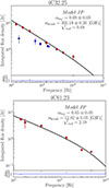 |
Fig. 7. Integrated radio spectra of 4C32.25 and 4C61.23. The flux densities are taken from the reduced datasets and the literature. The solid black line is the fit JP model. Red points are flux densities used in the fitting, while blue points are flux densities excluded from the fitting. The fit parameters and errors are indicated in the legend. |
Due to the limited number of observed flux density measurements available to fit the spectra of the components (primary lobes, wings), the injection indices were fixed to the corresponding values found for the integrated spectra. The only free parameter of the fits was νb. The flux densities for each component were calculated using manually defined DS9 regions. The flux densities were only extracted from the images mentioned in Section 3. The potential impact of different image resolutions on the flux density measurements was investigated. First, all images were re-gridded to the largest pixel scale and smoothed to a common resolution matching that of the NVSS image, which has the lowest resolution in our dataset. Next, we extracted the component flux densities and repeat the fitting process. We found that the differences in the fits were negligible, and we concluded that the variations in image resolution did not significantly affect our analysis. To maintain consistency with the previous fittings, we used the JP model to fit the radio spectra of all the components. These fittings are displayed in Fig. 8. The radio spectra of the wings of 4C32.25 exhibit spectral curvature, a key indicator of synchrotron aging, suggesting that these components are the oldest in 4C32.25. Table C.1 presents the derived physical properties and ages of 4C32.25 and 4C61.23.
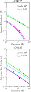 |
Fig. 8. Integrated radio spectra of the different components (primary lobes and wings) of 4C32.25 and 4C61.23. Colored points indicate the observed flux densities of the primary lobes (green and cyan), and wings (blue and purple). The solid green and cyan lines show the best-fit synchrotron model of the primary lobes, while the blue and purple lines show the best-fit synchrotron models of the wings, respectively. All the models are calculated keeping the injection index, αint fixed to the value indicated. |
We used Eq. (1) and the fit νb values to determine the spectral ages of the components. For 4C32.25, we found that the western and eastern primary lobes are the youngest components with inferred ages of 8.59 ± 0.34 Myr and 8.09 ± 0.61 Myr, respectively. The southern and northern wings are the oldest components with spectral ages of 82.16 ± 5.32 Myr and 90.77 ± 10.35 Myr, respectively. The northern wing could be older due to a more turbulent magnetic field (Klein et al. 1995). For 4C61.23, we found that southeastern and northwestern jets are the youngest components with spectral ages of 7.45 ± 0.55 Myr and 13.40 ± 1.74 Myr, respectively. Finally, the ages of the northeastern and southwestern wings are 7.66 ± 0.71 Myr and 14.11 ± 2.11 Myr, respectively.
In general, the spectral ages estimated for 4C32.25 and 4C61.23 agree with the expectations of precessional and backflow models (Leahy & Williams 1984; Parma et al. 1985; Mack et al. 1994), where the wings should be older than the primary lobes. For instance, Klein et al. (1995) found that the ages of the southern and northern wings are 69 Myr and 74 Myr, respectively. This implies that our age estimates agree within the uncertainties. Recently, Sebastian et al. (2024) estimated the spectral ages of 4C32.25 and 4C61.23 using only uGMRT maps at 400 and 1215 MHz. These authors calculated that for 4C61.23 (4C32.25) the ages of the primary lobes and wings are 37 Myr (51 Myr) and 30 Myr (22 Myr), respectively. These findings contradict our age estimates, as well the predictions of the models. This discrepancy could be explained by the fact that these authors had only two frequency measurements and assumed that the highest frequency in their data corresponded to the break frequency. Finally, our fittings included low-frequency observations, which are sensitive to diffuse, low-surface-brightness emission. This allowed us to detect the faint wings with higher significance and to determine the break frequency more precisely, thereby providing better estimates of the spectral ages.
6.1.3. Spectral index maps
The images described in Section 6.1.1 allowed us to investigate in detail the spectral index distributions of 4C32.25 and 4C61.23. The spectral index maps were determined using the standard expression for α = log(S1/S2)/log(ν1/ν2). Firstly, we found the largest pixel scale and lowest resolution of the image pair. Secondly, the images were re-gridded to the largest common pixel scale. Thirdly, the images were convolved with a Gaussian kernel to produce a circular PSF matching the size found in the first step. The uncertainties due to the flux density scale were added in quadrature, as described in Section 6.1.2.
The upper panels in Figure 9 presents the low-frequency and high-frequency spectral index maps of 4C32.25 derived between 150 MHz and 400 MHz,  , and between 400 MHz and 3.0 GHz,
  ; respectively. The maps only include pixels with flux densities above 3σ. Additionally, the spectral index profiles in both maps were calculated by integrating the flux density within 11 × 11 pixel boxes (2.75 times the beam size) placed along positions following the ridge of maximum brightness along the east-north (EN) and west-south (WS) directions from the primary lobes to the wings. The centers of the boxes are indicated with crosses in Figure 9. These profiles are displayed in the bottom panels of Figure 9. In the high-frequency spectral index map, the regions in the primary lobes exhibit values ranging from −0.82 to −0.74 with a steepening trend toward the start of the wings with typical values of −0.83. This gradual steepening of the high-frequency spectral index was also observed by Klein et al. (1995) and Rottmann (2001). To increase the S/N in the wings, we used larger box sizes of 15 × 15 pixels (3.75 times the beam size) to compute the flux densities in the 150 MHz and 400 MHz maps. In the
  map, the WS direction shows flat values of ∼ − 0.45 in the primary lobe region, with a sudden steepening occurring approximately in the latter half of the wing with values of ∼ − 1.0. The trend in the EN direction appears consistent with a steepening from the hot spot (∼ − 0.55) to the tip of the wing (∼ − 1.1), although the large error bars make it difficult to draw a definitive conclusion.
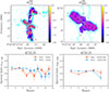 |
Fig. 9. Top row: Spectral index maps of 4C32.25 between 144−400 MHz (left) and 400−3000 MHz (right). The resolution of the maps is 10.1″ × 10.1″. The spectral index maps are derived using images from LOFAR/uGMRT (left) and uGMRT/VLA (right). The overlaid contour levels are [3, 12, 24, 48]×σrms, where σrms is the local noise from the corresponding lower frequency image. The locations of the centers of the boxes used to calculate the flux densities and corresponding spectral indices are indicated by the marked positions. Larger cross symbols correspond to areas where larger integration boxes were used for flux density estimation. Bottom row: Spectral index profiles of 4C32.25 along the east-north and west-south directions along the primary lobe to wing transition line computed from the spectral maps. The flux densities are calculated using 11 × 11 pixel boxes (2.75 times the beam size) in the primary lobe, and 15 × 15 pixel boxes (3.75 times the beam size) in the wings. In the spectral maps, the first and last boxes are indicated by number, with the locations of all boxes also displayed in the maps. The larger crosses in the 144−400 MHz spectral profiles denote that larger boxes were used to compute the flux densities. |
The low-frequency (150 MHz−400 MHz) and high-frequency (400 MHz−5.85 GHz) spectral index maps of 4C61.23 are shown in the upper panels of Figure 10. Flux densities were integrated using 6 × 6 pixel boxes (1.5 times the beam size). The south-east (SE) and north-west (NW) profiles (bottom panels of Figure 10) along the maximum brightness ridges obtained from the low-frequency spectral index map indicate a moderate and gradual steepening from the hot spots (∼ − 0.47) in the primary lobes to the tips of the wings (∼ − 0.55). In the high-frequency spectral index map, there is no significant change in the overall shape of the SE and NW profiles considering the associated uncertainties. The SE (NW) profile varies from −0.78 (−0.87) at the hot spot to −0.87 (−0.88) at the tip of the wing.
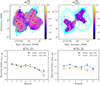 |
Fig. 10. Top row: Same as top row in Fig. 9, but for 4C61.23 using 4850 MHz instead of 3000 MHz as the highest frequency radio-map. The resolution of the maps is 11.1″ × 11.1″. The spectral index between 144−400 MHz map is displayed in the left, while the 400−4850 MHz map is shown in the right. Bottom row: Same as bottom row of Fig. 9, but for 4C61.23. The primary lobe to wing transition line is calculated along the south-east and north-west directions using the spectral index maps. The box size used is 6 × 6 pixels (1.5 times the beam size) to compute the flux densities. The first and last boxes are labeled in the spectral maps, with the positions of all boxes additionally displayed in the maps. |
6.2. Constraints on models derived from radio observations
The spectral ages and gradients found in Sections 6.1.2 and 6.1.3, respectively can be useful to constrain the formation models of 4C32.25 and 4C61.23. Particularly, in the jet reorientation (Parma et al. 1985; Mack et al. 1994) and backflow (Leahy & Williams 1984) models, it is expected that the wings are relic emission of previously active radio lobes. For instance, it has been proposed that jet precession could explain the radio morphology of 4C32.25 (Parma et al. 1985; Klein et al. 1995; Sebastian et al. 2024). On the other hand, the radio morphology of 4C61.23 suggests the wings are formed by strong backflows from both radio lobes, which are deflected in opposite directions perpendicular to the jet axis. This “double-boomerang” morphology has been explained in some XRGs using the backflow model (e.g., Cotton et al. 2020; Patra et al. 2023). Our spectral analyses of both XRGs yield older spectral ages for the wings and a gradual steepening from the young lobes to the old wings, as expected in the precession and backflow models, respectively. Also, Sebastian et al. (2024) proposed that precession could also explain the radio morphology of 4C61.23 with a precession period of 4.5 ≤ Pprec(Myr)≤70, which is compatible with our spectral age estimates.
Finally, a sudden reorientation of the jet axis, or a spin-flip event, could plausibly account for the radio morphology observed in some XRGs (Dennett-Thorpe et al. 2002; Merritt & Ekers 2002). For 4C61.23 and 4C32.25, the detection of double-peaked emission lines (Sebastian et al. 2024) suggests the presence of binary black holes (BBH), whose coalescence may have caused the sudden spin change (Merritt & Ekers 2002). VLBI observations support the presence of a BBH in 4C61.23 (Liu et al. 2018; Sebastian et al. 2024). However, for 4C61.23, jet-axis reorientation can be ruled out on radio-morphological grounds, as the wings appear to originate from backflow processes. For 4C32.25, the situation is different. First, we cannot reach the same conclusion as for 4C61.23, since no evidence of backflows is observed in 4C32.25. Second, the spin-flip scenario cannot be discarded, as a sudden jet reorientation may have occurred prior to the wings expanding to their current extent. Therefore, we conclude that more detailed observational and simulation studies are needed to understand the role of a spin-flip in shaping the radio morphology of 4C32.25.
6.3. Serendipitous radio sources
The discovery of serendipitous radio sources is important because it allows us to uncover previously unknown objects without requiring new observations (e.g., Oei et al. 2022; Norris et al. 2022). Furthermore, serendipitous discoveries maximize the scientific output of radio-surveys by providing information in target fields that were observed for other purposes. In this section, we discuss some serendipitous radio sources located in our XRGs fields and cross-reference them with the literature. Some of these sources lie beyond the first sidelobe of our mosaic, where beam attenuation affects the accuracy of their flux density measurements (Marr et al. 2015). Nevertheless, our images still revealed important morphological features that provide insights into the evolution of these radio sources. We calculated photometric redshifts for objects without spectroscopic confirmation. We used optical, and near and mid infrared photometry from the Pan-STARRS (Chambers et al. 2016), 2MASS (Skrutskie et al. 2006), and unWISE surveys (Schlafly et al. 2019), respectively. The coverage of the Legacy Survey (Dey et al. 2019) in our XRG fields is only partial, with some fields missing two bands. For this reason, we employed Pan-STARRS optical photometry to estimate the photometric redshifts. We followed the procedure described in Retana-Montenegro & Röttgering (2020) using the EAZY galaxy templates (Brammer et al. 2008) modified to take into account dust extinction in the host galaxies. Figures 11 and 12 display all the serendipitous sources included in our sample.
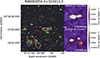 |
Fig. 11. Left: False color RGB (R = g, G = r, B = z) Legacy survey image (Dey et al. 2019) centered on the galaxy cluster RMJ083056.4+322412.2 located at zspec = 0.255. The image covers 600″ × 600″. The contours are [3, 5, 15, 20]×σ times the local noise level in the 400 MHz uGMRT map. The purple circle indicates the cluster center, and the red circles denote spectroscopically confirmed cluster members. Right: 400 MHz uGMRT image of two radio sources likely associated with RMJ083056.4+322412.2. The contour levels are the same as in the left panel. The beam size is shown in the white inset in the bottom left corner. |
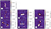 |
Fig. 12. Images showing the radio galaxies discussed in Section 6.3. The corresponding J2000 source names are indicated in the top center of each image. The beam size is shown in the white inset in the bottom left corner. The white bar in each image denotes indicates a scale of 1′. |
6.3.1. Galaxy cluster RMJ083056.4+322412.2
RMJ083056.4+322412.2 (RMJ0830) was first identified as an optically selected galaxy cluster candidate (Hao et al. 2010; Rykoff et al. 2014). The cluster redshift zspec = 0.255 was confirmed in the HeCS-red spectroscopic survey (Rines et al. 2018). The core of this cluster is 11.51′ from 4C32.25 (see Figure 11). Two extended radio sources, J083956.98+322415.7 and J083042.52+322708.6, appear to be associated with two clumps of spectroscopic cluster members near the cluster core. J083956.98+322415.7 was detected in previous observations of 4C32.25 (Parma et al. 1985; Mack et al. 1994; Klein et al. 1995), but it is only in this work that it has been associated with the cluster RMJ0830. The total flux densities are S400 MHz = 38.9 ± 5.87 mJy and S400 MHz = 210.9 ± 31 mJy, respectively. Both sources are also detected in the LoTSS (Shimwell et al. 2022) and NVSS (Condon et al. 1998) surveys.
6.3.2. Radio galaxy J201614.6–304130.7
As shown in Sect. 6.3, the radio galaxy J201614.6−304130.7 (also known as PKS 2013−308, Shimmins & Bolton 1974) is resolved at the resolution of the uGMRT band-3. The optical counterpart has a magnitude of iPS1 = 16 with a redshift of zspec = 0.088 (Jones et al. 2009). This radio galaxy has been observed over the course of several decades (Shimmins & Bolton 1974; Large et al. 1981, 1991; Jones & McAdam 1992). As the source lies beyond the first sidelobe, its flux density measurements in our mosaic are not accurate due to significant beam attenuation at that distance. The reported NVSS flux density is S1.4 GHz = 853.6 ± 15.5 mJy (Condon et al. 1998). The source is also detected in RACS maps (McConnell et al. 2020).
6.3.3. Radio galaxy J201123.9–302016.8
The optical counterpart is clearly identified between the radio lobes, with a redshift of zspec = 0.088 (Jones et al. 2009). No 400 MHz flux density is reported for this source because it lies beyond the first sidelobe in our mosaic. However, it has a total flux density of S1.4 GHz = 132.70 ± 4.3 mJy in the NVSS catalog (Condon et al. 1998), and it is detected in RACS maps (McConnell et al. 2020). This source exhibits asymmetric jets, with both jets showing signs of bending. Both bends are likely caused by the galaxy’s orbital motion, as well as interactions with the intergalactic medium, as seen previously in bent radio galaxies (Weżgowiec et al. 2024; Vardoulaki et al. 2025).
6.3.4. Radio galaxy J114113.4+61479.3
The radio source is associated with a Pan-STARRS source of iPS1 = 19.22 with a photometric redshift of zphoto = 0.46. The source displays an FRII-type radio morphology, characterized by asymmetric jets. The total flux densities are S400 MHz = 50.8 ± 7.6 mJy (this work) and S1.4 GHz = 63.4 ± 2.24 mJy (NVSS), respectively.
6.3.5. Radio galaxy J113321.5+61006.7
This radio source exhibits evidence of recurrent activity, resulting in a morphology reminiscent of that of double-double radio galaxies (DDRGs) with two pair of radio lobes (Saikia et al. 2006; Jamrozy et al. 2007). We associate this source with a faint optical source with iPS1 = 21.70 and with a photometric redshift of zphoto = 0.08 located between the inner double. We find that the total flux density in our mosaic is S400 MHz = 17.85 ± 4.3 mJy, while S1.4 GHz = 16 ± 0.9 mJy according to the NVSS catalog.
6.3.6. Radio galaxy J113106.3+611506.7
The radio source J113106.3+611506.7 (also known as 4C61.22, Pilkington & Scott 1965; Gower et al. 1967) was first discovered in the 4C survey (Gower et al. 1967). The radio structure of the source revealed by our 400 MHz maps consists of two bright lobes but with undistinguished core. The source is located beyond the first sidelobe in our mosaic thus its flux density cannot be determined reliably. The reported NVSS flux density is S1.4 GHz = 546.6 ± 13.80 mJy. The host galaxy, with iPS1 = 19.37, has been identified as the BCG of a galaxy cluster at zspec = 0.349 (Wen et al. 2012; Wen & Han 2015).
6.3.7. Extended radio source J083229.2+314234.3
Our 400 MHz mosaic reveals large-scale radio-emission surrounding a compact radio-core. There is a clear optical counterpart (iPS1 = 21.24 and zphoto = 0.49) coincident with the radio-peak of this source. Moreover, the diffuse component’s extension is also confirmed in the LoTSS images, where it appears fuzzier. We find that the total flux densities are S400 MHz = 13.50 ± 2.05 mJy, and S1.4 GHz = 5.6 ± 0.4 mJy as listed in the NVSS catalog. The extended emission associated with this optical source could be related to previous episodes of nonthermal nuclear activity as observed in fossil radio galaxies (Kempner et al. 2004; Riseley et al. 2023) and other galaxies (Kumari & Pal 2024a,b).
6.4. Radio galaxy J082556.5+31479.9
The source J082556.5+31479.9 (also known as B2 0822+31, Colla et al. 1970) shows a radio morphology with signatures of intermittent jet-formation in the form of two pairs of jets as seen in DDRGs (Schoenmakers et al. 2000; Mahatma et al. 2019; Nandi et al. 2019). The source location lies beyond the first sidelobe thus we do not determine its flux density using our mosaic. The listed NVSS flux density is S1.4 GHz = 162.2 ± 5.2 mJy. We find a unWISE counterpart (W1 = 18.07) at the expected location of the host galaxy between the pairs of inner lobes, but no optical counterpart in the Pan-STARRS images. This could indicate that there is significant dust obscuration in the host (e.g., Gabányi et al. 2021).
7. Summary and conclusions
In this paper, we used the extreme peeling calibration technique to produce wide-field and high-resolution uGMRT band-3 images. Our calibration approach assumes that the FOV can be divided into different regions, or facets, with each facet containing a source or source group that is bright enough to obtain high S/N calibration solutions. These solutions are applied, and the visibilities are imaged to obtain a new facet skymodel. Later, this skymodel is subtracted from the UV data. The process is iterated over all facets, allowing for the correction of DDES effects across the FOV. We conclude that this calibration method is robust enough to study not only the central XRG targets but also other diffuse radio sources located far from the field centers. This method could be extended to be used with other uGMRT bands. For instance, bands-4 and bands-5 have better angular resolution and reduced ionospheric effects, making the technique promising for detailed studies of compact AGN features. On the other hand, applying this approach to band-2 could help mitigate phase errors caused by stronger ionospheric distortions. Finally, our method offers a promising tool for calibrating both archival and future uGMRT observations of XRGs as well as other AGNs.
Our 400 MHz uGMRT images are combined with archival radio-data to perform a spectral analysis of 4C32.25 and 4C61.23 (see Sections 6.1.1, 6.1.2, 6.1.3, and 6.3). We find that the wings in 4C32.25 and 4C61.23 are the oldest components of the XRGs. The average spectral ages of the wings of the former is 79.03 ± 10.96 Myr, and that of the latter is 9.74 ± 1.93 Myr. In the spectral index map, we observe a steepening from the hotspots in the primary lobes toward the wings, consistent with the derived spectral ages. These estimates agree with previous results from the literature and align with the predictions from the precession and backflow models. Finally, we highlight several serendipitous radio sources found in our XRG fields and investigate their associations reported in the literature (Section 6.3). These radio sources include the galaxy cluster RMJ0830, as well as various radio galaxies showing signatures of intermittent jet activity and fossil radio-emission.
Data availability
Data for the mosaics and final catalogs of the fields 4C61.23, 4C32.25, and MRC 2011–298 are available at the CDS via https://cdsarc.cds.unistra.fr/viz-bin/cat/J/A+A/704/A137
Acknowledgments
The financial assistance of the South African Radio Astronomy Observatory (SARAO) towards this research is hereby acknowledged. We thank the anonymous referee for the helpful comments that improved this work. Computations were performed on Hippo at the University of KwaZulu-Natal, and at the Centre for High Performance Computing (project ASTR1534). We thank the staff of the GMRT that made these observations possible. GMRT is run by the National Centre for Radio Astrophysics of the Tata Institute of Fundamental Research. LOFAR, the Low Frequency Array designed and constructed by ASTRON, has facilities in several countries, that are owned by various parties (each with their own funding sources), and that are collectively operated by the International LOFAR Telescope (ILT) foundation under a joint scientific policy. The Open University is incorporated by Royal Charter (RC 000391), an exempt charity in England & Wales and a charity registered in Scotland (SC 038302). The Open University is authorized and regulated by the Financial Conduct Authority. This scientific work uses data obtained from Inyarrimanha Ilgari Bundara/the Murchison Radio-astronomy Observatory. We acknowledge the Wajarri Yamaji People as the Traditional Owners and native title holders of the Observatory site. CSIRO’s ASKAP radio telescope is part of the Australia Telescope National Facility (https://ror.org/05qajvd42). Operation of ASKAP is funded by the Australian Government with support from the National Collaborative Research Infrastructure Strategy. ASKAP uses the resources of the Pawsey Supercomputing Research Centre. Establishment of ASKAP, Inyarrimanha Ilgari Bundara, the CSIRO Murchison Radio-astronomy Observatory and the Pawsey Supercomputing Research Centre are initiatives of the Australian Government, with support from the Government of Western Australia and the Science and Industry Endowment Fund. This paper includes archived data obtained through the CSIRO ASKAP Science Data Archive, CASDA (https://data.csiro.au). The National Radio Astronomy Observatory is a facility of the National Science Foundation operated under cooperative agreement by Associated Universities, Inc. These work uses NVAS images that were produced as part of the NRAO VLA Archive Survey, (c) AUI/NRAO. The Pan-STARRS1 Surveys (PS1) have been made possible through contributions of the Institute for Astronomy, the University of Hawaii, the Pan-STARRS Project Office, the Max-Planck Society and its participating institutes, the Max Planck Institute for Astronomy, Heidelberg and the Max Planck Institute for Extraterrestrial Physics, Garching, The Johns Hopkins University, Durham University, the University of Edinburgh, Queen’s University Belfast, the Harvard-Smithsonian Center for Astrophysics, the Las Cumbres Observatory Global Telescope Network Incorporated, the National Central University of Taiwan, the Space Telescope Science Institute, the National Aeronautics and Space Administration under Grant No. NNX08AR22G issued through the Planetary Science Division of the NASA Science Mission Directorate, the National Science Foundation under Grant No. AST-1238877, the University of Maryland, and Eotvos Lorand University (ELTE). The Legacy Surveys consist of three individual and complementary projects: the Dark Energy Camera Legacy Survey (DECaLS; Proposal ID #2014B-0404; PIs: David Schlegel and Arjun Dey), the Beijing-Arizona Sky Survey (BASS; NOAO Prop. ID #2015A-0801; PIs: Zhou Xu and Xiaohui Fan), and the Mayall z-band Legacy Survey (MzLS; Prop. ID #2016A-0453; PI: Arjun Dey). DECaLS, BASS and MzLS together include data obtained, respectively, at the Blanco telescope, Cerro Tololo Inter-American Observatory, NSF’s NOIRLab; the Bok telescope, Steward Observatory, University of Arizona; and the Mayall telescope, Kitt Peak National Observatory, NOIRLab. Pipeline processing and analyses of the data were supported by NOIRLab and the Lawrence Berkeley National Laboratory (LBNL). The Legacy Surveys project is honored to be permitted to conduct astronomical research on Iolkam Duag (Kitt Peak), a mountain with particular significance to the Tohono O’odham Nation. This publication makes use of data products from the Wide-field Infrared Survey Explorer, which is a joint project of the University of California, Los Angeles, and the Jet Propulsion Laboratory/California Institute of Technology, funded by the National Aeronautics and Space Administration.
References
- Alexander, P., & Leahy, J. P. 1987, MNRAS, 225, 1 [NASA ADS] [CrossRef] [Google Scholar]
- Alexander, D. M., Hickox, R. C., Aird, J., et al. 2025, New Astron. Rev., 101, 101733 [Google Scholar]
- Andreon, S., Garilli, B., Maccagni, D., Gregorini, L., & Vettolani, G. 1992, A&A, 266, 127 [NASA ADS] [Google Scholar]
- Beck, R., & Krause, M. 2005, Astron. Nachr., 326, 414 [Google Scholar]
- Becker, R. H., White, R. L., & Helfand, D. J. 1995, ApJ, 450, 559 [Google Scholar]
- Bera, S., Sasmal, T. K., Patra, D., & Mondal, S. 2022, ApJS, 260, 7 [Google Scholar]
- Bhukta, N., Pal, S., & Mondal, S. K. 2022, MNRAS, 512, 4308 [Google Scholar]
- Brammer, G. B., van Dokkum, P. G., & Coppi, P. 2008, ApJ, 686, 1503 [Google Scholar]
- Brienza, M., Morganti, R., Harwood, J., et al. 2020, A&A, 638, A29 [EDP Sciences] [Google Scholar]
- Briggs, D. S. 1995, Ph.D. Thesis, New Mexico Institute of Mining and Technology [Google Scholar]
- Brunetti, G., Setti, G., & Comastri, A. 1997, A&A, 325, 898 [NASA ADS] [Google Scholar]
- Bruno, L., Gitti, M., Zanichelli, A., & Gregorini, L. 2019, A&A, 631, A173 [NASA ADS] [CrossRef] [EDP Sciences] [Google Scholar]
- Bruno, L., Brienza, M., Zanichelli, A., et al. 2024, A&A, 690, A160 [NASA ADS] [CrossRef] [EDP Sciences] [Google Scholar]
- Capetti, A., Zamfir, S., Rossi, P., et al. 2002, A&A, 394, 39 [NASA ADS] [CrossRef] [EDP Sciences] [Google Scholar]
- Chambers, K. C., Magnier, E. A., Metcalfe, N., et al. 2016, ArXiv e-prints [arXiv:1612.05560] [Google Scholar]
- Cheung, C. C. 2007, AJ, 133, 2097 [NASA ADS] [CrossRef] [Google Scholar]
- Clews, L., Croston, J. H., Dickinson, H., et al. 2025, MNRAS, 541, 3452 [Google Scholar]
- Cohen, A. S., Lane, W. M., Cotton, W. D., et al. 2007, AJ, 134, 1245 [Google Scholar]
- Colla, G., Fanti, C., Ficarra, A., et al. 1970, A&AS, 1, 281 [Google Scholar]
- Condon, J. J., Cotton, W. D., Greisen, E. W., et al. 1998, AJ, 115, 1693 [Google Scholar]
- Cotton, W. D., Thorat, K., Condon, J. J., et al. 2020, MNRAS, 495, 1271 [NASA ADS] [CrossRef] [Google Scholar]
- Coziol, R., Andernach, H., Caretta, C. A., Alamo-Martínez, K. A., & Tago, E. 2009, AJ, 137, 4795 [NASA ADS] [CrossRef] [Google Scholar]
- Crossley, J. H., Sjouwerman, L. O., Fomalont, E. B., & Radziwill, N. M. 2008, SPIE Conf. Ser., 7016, 70160O [Google Scholar]
- Dennett-Thorpe, J., Scheuer, P. A. G., Laing, R. A., et al. 2002, MNRAS, 330, 609 [NASA ADS] [CrossRef] [Google Scholar]
- Dey, A., Schlegel, D. J., Lang, D., et al. 2019, AJ, 157, 168 [Google Scholar]
- Duchesne, S. W., Thomson, A. J. M., Pritchard, J., et al. 2023, PASA, 40, e034 [NASA ADS] [CrossRef] [Google Scholar]
- Duchesne, S., Ross, K., Thomson, A. J. M., et al. 2025, PASA, 42, 38 [Google Scholar]
- Fanaroff, B. L., & Riley, J. M. 1974, MNRAS, 167, 31P [Google Scholar]
- Ferrarese, L., & Merritt, D. 2000, ApJ, 539, L9 [Google Scholar]
- Gabányi, K. É., Frey, S., & Perger, K. 2021, MNRAS, 506, 3641 [CrossRef] [Google Scholar]
- Giri, G., Fendt, C., Thorat, K., Bodo, G., & Rossi, P. 2024, Front. Astron. Space Sci., 11, 1371101 [NASA ADS] [CrossRef] [Google Scholar]
- Gopal-Krishna, & Chitre, S. M. 1983, Nature, 303, 217 [NASA ADS] [CrossRef] [Google Scholar]
- Gopal-Krishna, Biermann, P. L., Gergely, L. Á., & Wiita, P. J. 2012, RAA, 12, 127 [NASA ADS] [Google Scholar]
- Govoni, F., & Feretti, L. 2004, Int. J. Mod. Phys. D, 13, 1549 [Google Scholar]
- Gower, J. F. R., Scott, P. F., & Wills, D. 1967, MmRAS, 71, 49 [NASA ADS] [Google Scholar]
- Gregorini, L., Klein, U., Parma, P., Schlickeiser, R., & Wielebinski, R. 1992a, A&AS, 94, 13 [NASA ADS] [Google Scholar]
- Gregorini, L., Vettolani, G., de Ruiter, H. R., & Parma, P. 1992b, A&AS, 95, 1 [NASA ADS] [Google Scholar]
- Gregorini, L., de Ruiter, H. R., Parma, P., et al. 1994, A&AS, 106, 1 [NASA ADS] [Google Scholar]
- Gregory, P. C., & Condon, J. J. 1991, ApJS, 75, 1011 [Google Scholar]
- Greisen, E. W. 2003, Astrophys. Space Sci. Lib., 285, 109 [NASA ADS] [Google Scholar]
- Gupta, Y., Ajithkumar, B., Kale, H. S., et al. 2017, Curr. Sci., 113, 707 [NASA ADS] [CrossRef] [Google Scholar]
- Hale, C. L., McConnell, D., Thomson, A. J. M., et al. 2021, PASA, 38, e058 [NASA ADS] [CrossRef] [Google Scholar]
- Hao, J., McKay, T. A., Koester, B. P., et al. 2010, ApJS, 191, 254 [Google Scholar]
- Intema, H. T., van der Tol, S., Cotton, W. D., et al. 2009, A&A, 501, 1185 [NASA ADS] [CrossRef] [EDP Sciences] [Google Scholar]
- Intema, H. T., Jagannathan, P., Mooley, K. P., & Frail, D. A. 2017, A&A, 598, A78 [NASA ADS] [CrossRef] [EDP Sciences] [Google Scholar]
- Jaffe, W. J., & Perola, G. C. 1973, A&A, 26, 423 [NASA ADS] [Google Scholar]
- Jamrozy, M., Konar, C., Saikia, D. J., et al. 2007, MNRAS, 378, 581 [Google Scholar]
- Jones, P. A., & McAdam, W. B. 1992, ApJS, 80, 137 [CrossRef] [Google Scholar]
- Jones, D. H., Read, M. A., Saunders, W., et al. 2009, MNRAS, 399, 683 [Google Scholar]
- Joshi, R., Krishna, G., Yang, X., et al. 2019, ApJ, 887, 266 [NASA ADS] [CrossRef] [Google Scholar]
- Kardashev, N. S. 1962, Soviet Ast., 6, 317 [Google Scholar]
- Kempner, J. C., Blanton, E. L., Clarke, T. E., et al. 2004, in The Riddle of Cooling Flows in Galaxies and Clusters of Galaxies, eds. T. Reiprich, J. Kempner, & N. Soker, 335 [Google Scholar]
- Klein, U., Mack, K. H., Gregorini, L., & Parma, P. 1995, A&A, 303, 427 [Google Scholar]
- Kormendy, J., & Ho, L. C. 2013, ARA&A, 51, 511 [Google Scholar]
- Kumari, S., & Pal, S. 2024a, A&A, 683, A175 [NASA ADS] [CrossRef] [EDP Sciences] [Google Scholar]
- Kumari, S., & Pal, S. 2024b, MNRAS, 527, 11233 [Google Scholar]
- Lacy, M., Baum, S. A., Chandler, C. J., et al. 2020, PASP, 132, 035001 [Google Scholar]
- Lal, D. V., & Rao, A. P. 2007, MNRAS, 374, 1085 [NASA ADS] [CrossRef] [Google Scholar]
- Lal, D. V., Sebastian, B., Cheung, C. C., & Pramesh Rao, A. 2019, AJ, 157, 195 [NASA ADS] [CrossRef] [Google Scholar]
- Landt, H., Cheung, C. C., & Healey, S. E. 2010, MNRAS, 408, 1103 [NASA ADS] [CrossRef] [Google Scholar]
- Lara, L., Cotton, W. D., Feretti, L., et al. 2001a, A&A, 370, 409 [NASA ADS] [CrossRef] [EDP Sciences] [Google Scholar]
- Lara, L., Márquez, I., Cotton, W. D., et al. 2001b, A&A, 378, 826 [NASA ADS] [CrossRef] [EDP Sciences] [Google Scholar]
- Large, M. I., Mills, B. Y., Little, A. G., Crawford, D. F., & Sutton, J. M. 1981, MNRAS, 194, 693 [Google Scholar]
- Large, M. I., Cram, L. E., & Burgess, A. M. 1991, The Observatory, 111, 72 [NASA ADS] [Google Scholar]
- Leahy, J. P., & Parma, P. 1992, in Extragalactic Radio Sources. From Beams to Jets, eds. J. Roland, H. Sol, & G. Pelletier, 307 [Google Scholar]
- Leahy, J. P., & Williams, A. G. 1984, MNRAS, 210, 929 [CrossRef] [Google Scholar]
- Liu, X., Lazio, T. J. W., Shen, Y., & Strauss, M. A. 2018, ApJ, 854, 169 [Google Scholar]
- Mack, K. H., Gregorini, L., Parma, P., & Klein, U. 1994, A&AS, 103, 157 [Google Scholar]
- Magorrian, J., Tremaine, S., Richstone, D., et al. 1998, AJ, 115, 2285 [Google Scholar]
- Mahatma, V. H., Hardcastle, M. J., Williams, W. L., et al. 2019, A&A, 622, A13 [NASA ADS] [CrossRef] [EDP Sciences] [Google Scholar]
- Makarov, D., Prugniel, P., Terekhova, N., Courtois, H., & Vauglin, I. 2014, A&A, 570, A13 [NASA ADS] [CrossRef] [EDP Sciences] [Google Scholar]
- Marr, J. M., Snell, R. L., & Kurtz, S. E. 2015, Fundamentals of Radio Astronomy: Observational Methods (Series in Astronomy and Astrophysics) [Google Scholar]
- McConnell, D., Hale, C. L., Lenc, E., et al. 2020, PASA, 37, e048 [Google Scholar]
- McMullin, J. P., Waters, B., Schiebel, D., Young, W., & Golap, K. 2007, ASP Conf. Ser., 376, 127 [Google Scholar]
- Merritt, D., & Ekers, R. D. 2002, Science, 297, 1310 [NASA ADS] [CrossRef] [Google Scholar]
- Miley, G. 1980, ARA&A, 18, 165 [Google Scholar]
- Mohan, N., & Rafferty, D. 2015, Astrophysics Source Code Library [record ascl:1502.007] [Google Scholar]
- Morris, M. E., Wilcots, E., Hooper, E., & Heinz, S. 2022, AJ, 163, 280 [CrossRef] [Google Scholar]
- Nandi, S., Saikia, D. J., Roy, R., et al. 2019, MNRAS, 486, 5158 [CrossRef] [Google Scholar]
- Norris, R. P., Collier, J. D., Crocker, R. M., et al. 2022, MNRAS, 513, 1300 [NASA ADS] [CrossRef] [Google Scholar]
- Oei, M. S. S. L., van Weeren, R. J., Hardcastle, M. J., et al. 2022, A&A, 660, A2 [NASA ADS] [CrossRef] [EDP Sciences] [Google Scholar]
- Offringa, A. R., de Bruyn, A. G., Biehl, M., et al. 2010, MNRAS, 405, 155 [NASA ADS] [Google Scholar]
- Offringa, A. R., van de Gronde, J. J., & Roerdink, J. B. T. M. 2012, A&A, 539, A95 [NASA ADS] [CrossRef] [EDP Sciences] [Google Scholar]
- Offringa, A. R., de Bruyn, A. G., Zaroubi, S., et al. 2013, A&A, 549, A11 [NASA ADS] [CrossRef] [EDP Sciences] [Google Scholar]
- Offringa, A. R., McKinley, B., Hurley-Walker, N., et al. 2014, MNRAS, 444, 606 [Google Scholar]
- Oke, J. B., & Gunn, J. E. 1983, ApJ, 266, 713 [NASA ADS] [CrossRef] [Google Scholar]
- Pacholczyk, A. G. 1970, Radio Astrophysics. Nonthermal Processes in Galactic and Extragalactic Sources (San Francisco: Freeman) [Google Scholar]
- Parma, P., Ekers, R. D., & Fanti, R. 1985, A&AS, 59, 511 [NASA ADS] [Google Scholar]
- Patra, D., Joshi, R., & Gopal-Krishna 2023, MNRAS, 524, 3270 [NASA ADS] [Google Scholar]
- Pilkington, J. D. H., & Scott, J. F. 1965, MmRAS, 69, 183 [Google Scholar]
- Proctor, D. D. 2011, ApJS, 194, 31 [Google Scholar]
- Rees, M. J. 1978, Nature, 275, 516 [NASA ADS] [CrossRef] [Google Scholar]
- Rengelink, R. B., Tang, Y., de Bruyn, A. G., et al. 1997, A&AS, 124, 259 [NASA ADS] [CrossRef] [EDP Sciences] [Google Scholar]
- Retana-Montenegro, E. 2022, A&A, 663, A153 [NASA ADS] [CrossRef] [EDP Sciences] [Google Scholar]
- Retana-Montenegro, E., & Röttgering, H. 2020, A&A, 636, A12 [NASA ADS] [CrossRef] [EDP Sciences] [Google Scholar]
- Retana-Montenegro, E., Röttgering, H. J. A., Shimwell, T. W., et al. 2018, A&A, 620, A74 [NASA ADS] [CrossRef] [EDP Sciences] [Google Scholar]
- Reynolds, J. 1994, A Revised Flux Scale for the AT Compact Array, Tech. Rep. AT/39.3/040, ATNF [Google Scholar]
- Rines, K. J., Geller, M. J., Diaferio, A., Hwang, H. S., & Sohn, J. 2018, ApJ, 862, 172 [NASA ADS] [CrossRef] [Google Scholar]
- Riseley, C. J., Biava, N., Lusetti, G., et al. 2023, MNRAS, 524, 6052 [NASA ADS] [CrossRef] [Google Scholar]
- Rottmann, H. 2001, Ph.D. Thesis, University Bonn [Google Scholar]
- Rykoff, E. S., Rozo, E., Busha, M. T., et al. 2014, ApJ, 785, 104 [Google Scholar]
- Sabater, J., Best, P. N., Hardcastle, M. J., et al. 2019, A&A, 622, A17 [NASA ADS] [CrossRef] [EDP Sciences] [Google Scholar]
- Saikia, D. J., Konar, C., & Kulkarni, V. K. 2006, MNRAS, 366, 1391 [NASA ADS] [CrossRef] [Google Scholar]
- Saripalli, L., & Subrahmanyan, R. 2009, ApJ, 695, 156 [NASA ADS] [CrossRef] [Google Scholar]
- Scaife, A. M. M., & Heald, G. H. 2012, MNRAS, 423, L30 [Google Scholar]
- Schlafly, E. F., Meisner, A. M., & Green, G. M. 2019, ApJS, 240, 30 [Google Scholar]
- Schoenmakers, A. P., de Bruyn, A. G., Röttgering, H. J. A., van der Laan, H., & Kaiser, C. R. 2000, MNRAS, 315, 371 [Google Scholar]
- Schwab, F. R. 1984, AJ, 89, 1076 [NASA ADS] [CrossRef] [Google Scholar]
- Sebastian, B., Caproni, A., Kharb, P., et al. 2024, MNRAS, 530, 4902 [Google Scholar]
- Sekhar, S., & Athreya, R. 2018, AJ, 156, 9 [Google Scholar]
- Shimmins, A. J., & Bolton, J. G. 1974, Aust. J. Phys. Astrophys. Suppl., 32, 1 [Google Scholar]
- Shimwell, T. W., Röttgering, H. J. A., Best, P. N., et al. 2017, A&A, 598, A104 [NASA ADS] [CrossRef] [EDP Sciences] [Google Scholar]
- Shimwell, T. W., Hardcastle, M. J., Tasse, C., et al. 2022, A&A, 659, A1 [NASA ADS] [CrossRef] [EDP Sciences] [Google Scholar]
- Skrutskie, M. F., Cutri, R. M., Stiening, R., et al. 2006, AJ, 131, 1163 [NASA ADS] [CrossRef] [Google Scholar]
- Tasse, C. 2014, ArXiv e-prints [arXiv:1410.8706] [Google Scholar]
- Tasse, C., Hugo, B., Mirmont, M., et al. 2018, A&A, 611, A87 [NASA ADS] [CrossRef] [EDP Sciences] [Google Scholar]
- Tasse, C., Shimwell, T., Hardcastle, M. J., et al. 2021, A&A, 648, A1 [EDP Sciences] [Google Scholar]
- Ulrich, M. H., & Roennback, J. 1996, A&A, 313, 750 [Google Scholar]
- van der Laan, H., & Perola, G. C. 1969, A&A, 3, 468 [NASA ADS] [Google Scholar]
- van Diepen, G., Dijkema, T. J., & Offringa, A. 2018, Astrophysics Source Code Library [record ascl:1804.003] [Google Scholar]
- van Weeren, R. J., Williams, W. L., Hardcastle, M. J., et al. 2016, ApJS, 223, 2 [Google Scholar]
- Vardoulaki, E., Backöfer, V., Finoguenov, A., et al. 2025, A&A, 695, A178 [NASA ADS] [CrossRef] [EDP Sciences] [Google Scholar]
- Wen, Z. L., & Han, J. L. 2015, ApJ, 807, 178 [Google Scholar]
- Wen, Z. L., Han, J. L., & Liu, F. S. 2012, ApJS, 199, 34 [Google Scholar]
- Weżgowiec, M., Jamrozy, M., Chyży, K. T., et al. 2024, A&A, 691, A193 [NASA ADS] [CrossRef] [EDP Sciences] [Google Scholar]
- Williams, W. L., van Weeren, R. J., Röttgering, H. J. A., et al. 2016, MNRAS, 460, 2385 [Google Scholar]
- Xie, Z.-L., Bañados, E., Belladitta, S., et al. 2024, ApJ, 964, 98 [Google Scholar]
- Yang, X., Joshi, R., Gopal-Krishna, et al. 2019, ApJS, 245, 17 [CrossRef] [Google Scholar]
- Yang, X., Ji, J., Joshi, R., et al. 2022, ApJ, 933, 98 [Google Scholar]
Appendix A: Corrected positional offsets and total flux comparison of the three X-shaped radio galaxies fields
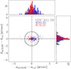 |
Fig. A.1. The corrected positional offsets between high S/N and compact uGMRT sources and their FIRST/RACS (Becker et al. 1995; McConnell et al. 2020) counterparts. The dashed lines denote a circle with radius r = 2″, which is the mosaic pixel scale. The colored ellipses centered on the right ascension and declination mean offsets indicate the standard deviation for both directions. |
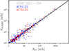 |
Fig. A.2. Total flux densities of matches between our 400 MHz uGMRT catalogs and the reference surveys LoTSS and RACS (Shimwell et al. 2022; McConnell et al. 2020) The dashed line indicates a flux density ratio equal to unity. A correction factor is applied to the RACS flux densities to convert them from the Reynolds (1994) scale to the SH12 flux density scale adopted in this work. |
In Figure A.1, we show the corrected positional offsets between high S/N and compact uGMRT sources and their counterparts in the reference high-resolution surveys FIRST/RACS (Becker et al. 1995; McConnell et al. 2020). Figure A.2 shows the flux density scale comparison between the scaled uGMRT and the reference flux densities at 400 MHz. The methods to correct the astrometry and flux densities are described in RM18.
Appendix B: Flux densities of 4C32.25, 4C61.23, and MRC 2011-298.
Table B.1 reports the total flux densities of 4C32.25, and 4C61.23 compiled from the literature and this work to fit the integrated spectra of 4C32.25 and 4C61.23 in Section 6.1.2. Table B.2 presents the 400 MHz flux densities of the different components of MRC 2011-298 estimated using the radio-map from Section 5.
Total flux densities of 4C32.25 and 4C61.23
Flux densities of the various components of MRC 2011-298 measured at 400 MHz.
Appendix C: Physical properties and spectral ages of 4C32.25 and 4C61.23
Table C.1 reports the physical properties and spectral ages derived in Section 6.1.2.
Physical properties and ages of 4C32.25 and 4C61.23.
All Tables
All Figures
|
Fig. 1. Fit clock differences using the gain solutions from 3C147. The values show a bimodal distribution between core and arm antennas (mainly from the southern arm). The colors represent different antennas. |
| In the text | |
|
Fig. 2. Schematic view of the direction-independent calibration steps for uGMRT Band 3 data. |
| In the text | |
|
Fig. 3. Schematic view of the direction-dependent calibration steps for uGMRT Band 3 data. |
| In the text | |
|
Fig. 4. The spatial distribution of facets in the 4C61.23, 4C25.25, and MRC 2011–298 fields. The blue circle denotes angular distance where the uGMRT beam is 50% of that at the pointing center; that is, about 0.74°. |
| In the text | |
|
Fig. 5. Images showing a direction-dependent self-calibration sequence for facet calibrators from the different fields. The corresponding field name is indicated in the images of the first column. The first column displays the images made with only the DI self-calibration solutions. The central column displays the improvements after two iterations of fast phase (TEC and phase-offset)-only DDE calibration. The right-hand column shows the improvement after two further iterations of fast phase (TEC+phase offset) and slow phase and amplitude (XX and YY gain) DDE calibration. The scale is the same for all images of the self-calibration sequence. |
| In the text | |
|
Fig. 6. Right: 400 MHz uGMRT mosaics of the 4C32.25, 4C61.23, and MRC 2011–298 fields. The area of each mosaic is approximately 1.72 deg2. The details of each field are summarized in Table 2. Left: Full-resolution uGMRT 400 MHz band-3 images of the three XRGs 4C32.25, 4C61.23, and MRC 2011–298. The contour levels are (1, 2, 4, 8, …)×3σ mJy/beam, where σ is the local noise level. The −3σ contours are denoted by dashed lines. The restoring beam is indicated by an ellipse in the bottom left corner. The black line indicates the corresponding angular scale. |
| In the text | |
|
Fig. 7. Integrated radio spectra of 4C32.25 and 4C61.23. The flux densities are taken from the reduced datasets and the literature. The solid black line is the fit JP model. Red points are flux densities used in the fitting, while blue points are flux densities excluded from the fitting. The fit parameters and errors are indicated in the legend. |
| In the text | |
|
Fig. 8. Integrated radio spectra of the different components (primary lobes and wings) of 4C32.25 and 4C61.23. Colored points indicate the observed flux densities of the primary lobes (green and cyan), and wings (blue and purple). The solid green and cyan lines show the best-fit synchrotron model of the primary lobes, while the blue and purple lines show the best-fit synchrotron models of the wings, respectively. All the models are calculated keeping the injection index, αint fixed to the value indicated. |
| In the text | |
|
Fig. 9. Top row: Spectral index maps of 4C32.25 between 144−400 MHz (left) and 400−3000 MHz (right). The resolution of the maps is 10.1″ × 10.1″. The spectral index maps are derived using images from LOFAR/uGMRT (left) and uGMRT/VLA (right). The overlaid contour levels are [3, 12, 24, 48]×σrms, where σrms is the local noise from the corresponding lower frequency image. The locations of the centers of the boxes used to calculate the flux densities and corresponding spectral indices are indicated by the marked positions. Larger cross symbols correspond to areas where larger integration boxes were used for flux density estimation. Bottom row: Spectral index profiles of 4C32.25 along the east-north and west-south directions along the primary lobe to wing transition line computed from the spectral maps. The flux densities are calculated using 11 × 11 pixel boxes (2.75 times the beam size) in the primary lobe, and 15 × 15 pixel boxes (3.75 times the beam size) in the wings. In the spectral maps, the first and last boxes are indicated by number, with the locations of all boxes also displayed in the maps. The larger crosses in the 144−400 MHz spectral profiles denote that larger boxes were used to compute the flux densities. |
| In the text | |
|
Fig. 10. Top row: Same as top row in Fig. 9, but for 4C61.23 using 4850 MHz instead of 3000 MHz as the highest frequency radio-map. The resolution of the maps is 11.1″ × 11.1″. The spectral index between 144−400 MHz map is displayed in the left, while the 400−4850 MHz map is shown in the right. Bottom row: Same as bottom row of Fig. 9, but for 4C61.23. The primary lobe to wing transition line is calculated along the south-east and north-west directions using the spectral index maps. The box size used is 6 × 6 pixels (1.5 times the beam size) to compute the flux densities. The first and last boxes are labeled in the spectral maps, with the positions of all boxes additionally displayed in the maps. |
| In the text | |
|
Fig. 11. Left: False color RGB (R = g, G = r, B = z) Legacy survey image (Dey et al. 2019) centered on the galaxy cluster RMJ083056.4+322412.2 located at zspec = 0.255. The image covers 600″ × 600″. The contours are [3, 5, 15, 20]×σ times the local noise level in the 400 MHz uGMRT map. The purple circle indicates the cluster center, and the red circles denote spectroscopically confirmed cluster members. Right: 400 MHz uGMRT image of two radio sources likely associated with RMJ083056.4+322412.2. The contour levels are the same as in the left panel. The beam size is shown in the white inset in the bottom left corner. |
| In the text | |
|
Fig. 12. Images showing the radio galaxies discussed in Section 6.3. The corresponding J2000 source names are indicated in the top center of each image. The beam size is shown in the white inset in the bottom left corner. The white bar in each image denotes indicates a scale of 1′. |
| In the text | |
|
Fig. A.1. The corrected positional offsets between high S/N and compact uGMRT sources and their FIRST/RACS (Becker et al. 1995; McConnell et al. 2020) counterparts. The dashed lines denote a circle with radius r = 2″, which is the mosaic pixel scale. The colored ellipses centered on the right ascension and declination mean offsets indicate the standard deviation for both directions. |
| In the text | |
|
Fig. A.2. Total flux densities of matches between our 400 MHz uGMRT catalogs and the reference surveys LoTSS and RACS (Shimwell et al. 2022; McConnell et al. 2020) The dashed line indicates a flux density ratio equal to unity. A correction factor is applied to the RACS flux densities to convert them from the Reynolds (1994) scale to the SH12 flux density scale adopted in this work. |
| In the text | |
Current usage metrics show cumulative count of Article Views (full-text article views including HTML views, PDF and ePub downloads, according to the available data) and Abstracts Views on Vision4Press platform.
Data correspond to usage on the plateform after 2015. The current usage metrics is available 48-96 hours after online publication and is updated daily on week days.
Initial download of the metrics may take a while.