| Issue |
A&A
Volume 704, December 2025
|
|
|---|---|---|
| Article Number | A41 | |
| Number of page(s) | 20 | |
| Section | Planets, planetary systems, and small bodies | |
| DOI | https://doi.org/10.1051/0004-6361/202556791 | |
| Published online | 05 December 2025 | |
Mass determination of the three long-period Neptune- and sub-Neptune-sized planets transiting TOI-282★
1
Dipartimento di Fisica, Università degli Studi di Torino,
via Pietro Giuria 1,
10125
Torino,
Italy
2
European Southern Observatory,
Alonso de Cordova 3107, Vitacura,
Santiago de Chile,
Chile
3
Space Research Institute, Austrian Academy of Sciences,
Schmiedlstraße 6,
8042
Graz,
Austria
4
Dipartimento di Fisica, Università di Trento,
Via Sommarive 14,
38123
Povo,
Italy
5
Dipartimento di Fisica e Astronomia “Galileo Galilei”, Università degli Studi di Padova,
Vicolo dell’Osservatorio 3,
35122
Padova,
Italy
6
Leiden Observatory, University of Leiden,
PO Box 9513,
2300
RA
Leiden,
The Netherlands
7
Department of Space, Earth and Environment, Chalmers University of Technology, Onsala Space Observatory,
439 92
Onsala,
Sweden
8
Osservatorio Astrofisico di Torino, INAF,
via Osservatorio 20,
Pino Torinese
10025,
Italy
9
McDonald Observatory and Department of Astronomy, The University of Texas at Austin,
USA
10
Center for Planetary Systems Habitability, The University of Texas at Austin,
USA
11
Institute of Astronomy, Faculty of Physics, Astronomy and Informatics, Nicolaus Copernicus University,
Grudziądzka 5,
87-100
Toruń,
Poland
12
Instituto de Astrofísica de Canarias, Vía Láctea s/n,
38200
La Laguna, Tenerife,
Spain
13
Departamento de Astrofísica, Universidad de La Laguna, Astrofísico Francisco Sanchez s/n,
38206
La Laguna, Tenerife,
Spain
14
Astronomy Department and Van Vleck Observatory, Wesleyan University,
Middletown,
CT
06459,
USA
15
Rheinisches Institut für Umweltforschung an der Universität zu Köln,
Aachener Straße 209,
50931
Köln,
Germany
16
Institute of Space Research, German Aerospace Center (DLR),
Rutherfordstraße 2,
12489
Berlin,
Germany
17
Astrobiology Center, NINS,
2-21-1 Osawa, Mitaka,
Tokyo
181-8588,
Japan
18
National Astronomical Observatory of Japan, NINS,
2-21-1 Osawa, Mitaka,
Tokyo
181-8588,
Japan
19
Astronomical Science Program Graduate University for Advanced Studies, SOKENDAI,
2-21-1, Osawa, Mitaka,
Tokyo,
181-8588,
Japan
★★ Corresponding author: This email address is being protected from spambots. You need JavaScript enabled to view it.
Received:
8
August
2025
Accepted:
23
October
2025
Abstract
TOI-282 is a bright (V = 9.38) F8 main-sequence star known to host three transiting long-period (Pb = 22.9 d, Pc = 56.0 d, and Pd = 84.3 d) small (Rp ≈ 2–4 R⊕) planets. The orbital period ratio of the two outermost planets, namely TOI-282 c and d, is close to the 3:2 commensurability, suggesting that the planets might be trapped in a mean motion resonance. We combined space-borne photometry from the TESS telescope with high-precision HARPS and ESPRESSO Doppler measurements to refine orbital parameters, measure the planetary masses, and investigate the architecture and evolution of the system. We performed a Markov chain Monte Carlo joint analysis of the transit light curves and radial velocity time series, and carried out a dynamical analysis to model transit timing variations and Doppler measurements along with N-body integration. In agreement with previous results, we found that TOI-282 b, c, and d have radii of Rb = 2.69 ± 0.23 R⊕, Rc = 4.13−0.14+0.16 R⊕, and Rd = 3.11 ± 0.15 R⊕, respectively. We measured planetary masses of Mb = 6.2 ± 1.6 M⊕, Mc = 9.2 ± 2.0 M⊕, and Md = 5.8−1.1+0.9 M⊕, which imply mean densities of ρb = 1.8−0.6+0.7 g cm−3, ρc = 0.7 ± 0.2 g cm−3, and ρd = 1.1−0.2+0.3 g cm−3, respectively. The three planets may be water worlds, making TOI-282 an interesting system for future atmospheric follow-up observations with JWST and ELT.
Key words: planets and satellites: composition / planets and satellites: dynamical evolution and stability / planets and satellites: fundamental parameters / planets and satellites: general / planets and satellites: physical evolution
Based on observations performed at the European Southern Observatory under programmes 60.A-9700, 60.A-9709, 0104.C-0003, 106.21TJ.001, and 108.22EH.001.
© The Authors 2025
 Open Access article, published by EDP Sciences, under the terms of the Creative Commons Attribution License (https://creativecommons.org/licenses/by/4.0), which permits unrestricted use, distribution, and reproduction in any medium, provided the original work is properly cited.
This article is published in open access under the Subscribe to Open model. This email address is being protected from spambots. You need JavaScript enabled to view it. to support open access publication.
1 Introduction
Multi-planet systems are remarkable laboratories for investigating the nature of planets orbiting stars other than the Sun. They provide a unique opportunity to ‘freeze’ the age and chemical composition of the star and its planet-forming disk, which are crucial parameters to study planetary formation and evolution. This enables direct comparisons among the planets within a single system, enabling the investigation of their architecture and mutual gravitational interactions, ultimately providing valuable insights into their formation and evolutionary pathways (e.g. Petrovich et al. 2020; Weiss et al. 2022; Mishra et al. 2023; Leleu et al. 2024; Howe et al. 2025). We can also compare different planetary systems to study patterns as a function of their parameters, such as stellar spectral type, age, and instellation (e.g. Gupta &a Schlichting 2020; Spaargaren et al. 2020; Luque & Pallé 2022; Rogers et al. 2023; Venturini et al. 2024). This is only possible by precisely and accurately characterising the planets within the system. Deriving radii and masses of planets, and consequently bulk densities, allows us to study their internal structure and composition, providing important hints about their formation and evolution (Winn & Fabrycky 2015).
Among the various types of exoplanets discovered to date, super-Earths (1 ≲ Rp ≲ 2 R⊕) and sub-Neptunes (2 ≲ Rp ≲ 4 R⊕) stand out as the most intriguing ones. These planets are not present in our Solar System, yet they are found orbiting around nearly half of the solar-like stars in the Galaxy (Batalha et al. 2013; Petigura et al. 2013; Marcy et al. 2014; Zang et al. 2025). Investigating their nature and properties is of particular interest, as it may help us to put into context the apparent uniqueness of our Solar System and further explore their peculiar demographics.
Long-period (P ≳ 50 d) transiting sub-Neptunes offer a unique opportunity to investigate the properties of exoplanet atmospheres that remain largely unaffected by tidal interactions with their host stars and/or by stellar irradiation. Residing in cooler environments, their chemical and dynamical processes may resemble those of the Solar System’s planets, making them compelling targets for exploring atmospheric diversity (Giacobbe et al. 2021). Moreover, transiting long-period sub-Neptunes are ideal candidates for atmospheric characterisation with the James Webb Space Telescope (JWST; Gardner et al. 2006), which might even lead to the discovery of biosignatures (e.g. Madhusudhan et al. 2016; Madhusudhan 2019; Kempton & Knutson 2024).
Although the number of confirmed exoplanets has increased to more than 60001, only ~20% of these have orbital periods exceeding 50 d. Narrowing down to long-period transiting sub-Neptunes (P ≳ 50 d and 2 ≲ Rp ≲ 4 R⊕), this percentage falls to ~5%, due to the well-known observational biases of the radial velocity and transit methods (Winn & Fabrycky 2015). Characterising the existing relatively small sample of transiting long-period sub-Neptunes represents a key step towards comprehending their formation and evolution processes.
Here we present the characterisation of the multi-planet system TOI-282 (aka HD 28109), a bright (V = 9.38), mainsequence star of spectral type F8 known to host three transiting long-period Neptunian planets, namely TOI-282b (Pb ≈ 22.9 d, Rb ≈ 2.2 R⊕), TOI-282c (Pc ≈ 56.0 d, Rc ≈ 4.2 R⊕), and TOI-282 d (Pd ≈ 84.3 d, Rd ≈ 3.3 R⊕). The discovery of the system has been announced by Dransfield et al. 2022 (hereafter D22), who combined TESS space-borne photometry with ground-based transit observations to determine the orbital period and radius of each planet. With the aim of measuring the masses of the three planets, we carried out intensive radial velocity (RV) follow-up observations of the star using the HARPS and ESPRESSO spectrographs and jointly modelled the Doppler measurements with TESS transit photometry.
The paper is organised as follows. Sect. 2 presents the photometric and spectroscopic data. Sect. 3 describes our determination of the fundamental parameters of the star TOI-282. Appendix A outlines the frequency analysis of the RV and activity indicator time series. After describing the data modelling in Appendix 4, we present the planetary parameters (Sect. 5) and a dynamical analysis (Sect. 6). Finally, discussions and conclusions are provided in Sects. 7 and 8, respectively.
2 Observations and data reduction
2.1 TESS photometry
The photometric analysis presented in this paper is exclusively based on publicly available TESS (Ricker et al. 2015) space-borne photometry, which we retrieved from the STScI Mikulski Archive for Space Telescope2 (MAST). As of June 2025, TESS has observed TOI-282 in 37 sectors, namely, sectors 1–13, 27–31, 33–39, 61–69, and 87–90. The TESS observations used in the present paper cover a baseline of nearly 7 years, from July 2018 to March 2025. The results presented in D22 are based on the first 23 TESS sectors (July 2018-April 2021; sectors 1–13, 27–31, and 33–37).
We downloaded the two-minute cadence light curves (LCs) as processed and calibrated by the Science Processing Operations Center (SPOC; Jenkins et al. 2016) at NASA Ames Research Center. For our analysis, we used the data products delivered in the form of Presearch Data Conditioning Simple Aperture Photometry (PDCSAP; Smith et al. 2012; Stumpe et al. 2012), which is corrected for instrumental artefacts, systematic trends, and contaminations. We discarded those data points with poor quality flags and extracted ~4 hours of out-of-transit photometry both before and after each transit for de-trending purposes. Our photometric data set comprises 59 transit LCs, which are broken down as follows: 33, 18, and 8 transits for TOI-282b, c, and d, respectively. The 59 transit LCs contain time stamps in barycentric Julian dates in barycentric dynamical time (BJDTDB; Eastman et al. 2010), along with the corresponding PDCSAP fluxes and uncertainties. The time series includes the following ancillary vectors that are part of the TESS science data product: mom_centr1, mom_centr2, pos_corr1, and pos_corr2.
2.2 HARPS spectroscopy
We started the RV follow-up of TOI-282 using the High Accuracy Radial Velocity Planet Searcher (HARPS; Mayor et al. 2003) echelle spectrograph installed on the ESO 3.6-m telescope at La Silla Observatory, Chile. Two high-resolution (R ≈ 115 000) spectra of TOI-282 were acquired on 21 and 22 February 2019 (program ID 60.A-9700). We collected 36 additional spectra between 6 December 2020 and 17 July 2021 (program IDs 60.A-9709 and 106.21TJ.001; PI: D. Gandolfi). The observations were carried out as part of our intensive RV follow-up program of TESS small transiting planets conducted with the HARPS spectrograph (see, e.g. Gandolfi et al. 2025). The exposure time was set to 1500–1800 s, which resulted in a median signal-to-noise ratio (S/N) of ~104 per pixel at 550 nm. One spectrum was discarded due to contamination from scattered moonlight, leading to 37 useful HARPS spectra.
We reduced the spectra using the dedicated HARPS data reduction software (DRS; Lovis & Pepe 2007) and computed the cross-correlation functions (CCFs) using a G2 numerical mask (Baranne et al. 1996; Pepe et al. 2002). We also utilised the DRS to extract the log ![Mathematical equation: $\[\mathrm{R}_{\mathrm{HK}}^{\prime}\]$](/articles/aa/full_html/2025/12/aa56791-25/aa56791-25-eq5.png) chromospheric index from the Ca II H & K lines (Table B.2). Following the methodology described in Simola et al. (2019), we fitted a skew-normal (SN) function to the HARPS CCFs to extract the RV measurements along with three profile diagnostics of the SN function, namely, the full width at half maximum FWHM, the contrast A, and the skewness γ (Table B.1). The RV uncertainties σRV were derived from the variance-covariance matrix of the model parameters following Richter (1995). We finally extracted the Na D1, Na D2, and Hα lines activity indicators (Table B.2) using the Template Enhanced Radial Velocity Re-analysis Application (TERRA; Anglada-Escudé & Butler 2012).
chromospheric index from the Ca II H & K lines (Table B.2). Following the methodology described in Simola et al. (2019), we fitted a skew-normal (SN) function to the HARPS CCFs to extract the RV measurements along with three profile diagnostics of the SN function, namely, the full width at half maximum FWHM, the contrast A, and the skewness γ (Table B.1). The RV uncertainties σRV were derived from the variance-covariance matrix of the model parameters following Richter (1995). We finally extracted the Na D1, Na D2, and Hα lines activity indicators (Table B.2) using the Template Enhanced Radial Velocity Re-analysis Application (TERRA; Anglada-Escudé & Butler 2012).
2.3 ESPRESSO spectroscopy
We also observed TOI-282 using the Echelle SPectrograph for Rocky Exoplanet and Stable Spectroscopic Observations (ESPRESSO; Pepe et al. 2014, 2021) installed on the 8.2-m ESO Very Large Telescope (VLT) at Paranal Observatory, Chile. The observations were carried out as part of two dedicated ESPRESSO programs to spectroscopically follow up TOI-282 (program IDs 0104.C-0003 and 108.22EH.001; PI: F. Rodler). We acquired 44 high-resolution (R ≈ 140 000) spectra covering a baseline of nearly 2.5 years, between October 2019 and March 2022. We set the exposure time to 935–1270 s, achieving a median S/N of 122 per pixel at 550 nm. In November and December 2020, ESPRESSO underwent an upgrade of the Fabry-Pérot lamp. To account for a possible RV offset resulting from the instrument refurbishment, we split the data into ESPRESSO 1st and 2nd sets. The former is composed of 8 spectra acquired between 15 October and 27 December 2019, whereas the latter includes the remaining 36 spectra that were secured between 5 October 2021 and 2 March 2022. As performed with HARPS data (Sect. 2.2), we reduced the ESPRESSO spectra with the dedicated DRS (Pepe et al. 2021), computed the CCFs using a F9 mask, and extracted the RV measurements and profile diagnostics by fitting an SN function to the ESPRESSO CCFs (Table B.3).
3 Stellar characterisation
3.1 Spectroscopic parameters
We derived the spectroscopic parameters of TOI-282 from the co-added ESPRESSO spectrum, which has a S/N of ~1400 per pixel at 550 nm. (Sect. 2.3). The modelling of the spectrum was performed with the code Spectroscopy Made Easy3 (SME, version 5.2.2; Valenti & Piskunov 1996; Piskunov & Valenti 2017), along with synthetic spectra generated using ATLAS12 atmospheric models (Kurucz 2013). SME automatically computes synthetic spectra and compares them with the observed spectrum to derive the spectroscopic parameters. We modelled one parameter at a time, utilising spectral features sensitive to different photospheric parameters, and iterating until convergence of all parameters was reached. We measured the projected rotational velocity v sin i⋆ by simultaneously fitting unblended iron lines. Throughout the modelling, we kept the macro- and micro-turbulent velocities (vmac and vmic) fixed to 4.1 km s−1 (Doyle et al. 2014) and 1.2 km s−1 (Bruntt et al. 2008), respectively. An exhaustive description of the procedure is provided in Persson et al. (2018). Our results are listed in Table 1.
As a sanity check, we used the code specmatch-emp4 (Yee et al. 2017), which derives the spectroscopic parameters by comparing observed spectra with a grid of nearly 400 high-resolution, high S/N template spectra acquired with the HIRES spectrograph. Prior to executing specmatch-emp, we lowered the resolution and adjusted the format of the ESPRESSO co-added spectrum to ensure compatibility with the HIRES template spectra. This analysis provides an effective temperature of Teff = 5980 ± 110 K, in fairly good agreement with the SME results. We also employed the spectral energy distribution (SED) fitting software astroARIADNE5 (Vines & Jenkins 2022) to measure the interstellar reddening along the line of sight to the star and derive a first estimate of the stellar radius. We used the spectroscopic parameters derived with SME and the broad-band magnitudes listed in Table 1, along with the Gaia DR3 offset-corrected parallax ϖ (Gaia Collaboration 2023; Lindegren et al. 2021). We fitted the SED using three different atmospheric model grids from Phoenix v2 (Husser et al. 2013), Castelli & Hubrig (2004), and Kurucz (1993). The radius and visual extinction were calculated via Bayesian model averaging. We found that the star has a radius of R⋆ = 1.46 ± 0.02 R⊙ and suffers a negligible reddening of Av = 0.06 ± 0.04.
Main identifiers, equatorial coordinates, parallax, distance, optical and near-infrared magnitudes, and fundamental parameters of the star TOI-282.
3.2 Stellar luminosity, mass, radius, and age
To refine the stellar radius R⋆ and derive the luminosity L⋆, mass M⋆, and age t⋆, we followed the multi-photometric approach described in Bonfanti et al. (2025). Briefly, for each broadband magnitude listed in Table 1, we first built an input set of parameters made of the SME-derived Teff, [M/H], and log g⋆, along with the Gaia DR3 offset-corrected parallax ϖ. We then interpolated pre-computed grids of PARSEC6 v1.2S isochrones and tracks (Marigo et al. 2017) via the isochrone placement routine (Bonfanti et al. 2015, 2016) by using each input set as a constraint. We ended up with ten different sets of estimates for L⋆, R⋆, M⋆, and t⋆ (one for each input magnitude). After checking the mutual consistency of the results via the χ2−based criterion outlined in Bonfanti et al. (2021), we merged the respective distributions and determined L⋆ = ![Mathematical equation: $\[2.71_{-0.14}^{+0.16}\]$](/articles/aa/full_html/2025/12/aa56791-25/aa56791-25-eq9.png) L⊙, R⋆ =
L⊙, R⋆ = ![Mathematical equation: $\[1.425_{-0.041}^{+0.048}\]$](/articles/aa/full_html/2025/12/aa56791-25/aa56791-25-eq10.png) R⊙, M⋆ = 1.227 ± 0.052 M⊙, and t⋆ = 3.2 ± 0.9 Gyr (Table 1). The stellar radius is in agreement with that obtained using astroARIADNE, corroborating our results. Assuming that TOI-282 is seen equator-on (i⋆ = 90°), the stellar radius and projected rotational velocity (Table 1) imply a rotation period of Prot,⋆ = 9.1 ± 0.7 d. Based on the B − V = 0.53 ± 0.04 colour index and the median log
R⊙, M⋆ = 1.227 ± 0.052 M⊙, and t⋆ = 3.2 ± 0.9 Gyr (Table 1). The stellar radius is in agreement with that obtained using astroARIADNE, corroborating our results. Assuming that TOI-282 is seen equator-on (i⋆ = 90°), the stellar radius and projected rotational velocity (Table 1) imply a rotation period of Prot,⋆ = 9.1 ± 0.7 d. Based on the B − V = 0.53 ± 0.04 colour index and the median log ![Mathematical equation: $\[\mathrm{R}_{\mathrm{HK}}^{\prime}\]$](/articles/aa/full_html/2025/12/aa56791-25/aa56791-25-eq11.png) = −4.991 ± 0.003 (Table 1), the rotation-activity empirical relations from Mamajek & Hillenbrand (2008) and Suárez Mascareño et al. (2016) provide a rotation period of 12 ± 2 d and 13 ± 5 d, respectively, which are consistent with the value we estimated from v sin i⋆.
= −4.991 ± 0.003 (Table 1), the rotation-activity empirical relations from Mamajek & Hillenbrand (2008) and Suárez Mascareño et al. (2016) provide a rotation period of 12 ± 2 d and 13 ± 5 d, respectively, which are consistent with the value we estimated from v sin i⋆.
Dransfield et al. (2022) derived a gyro-chronological age of 1.1 ± 0.1 Gyr for TOI-282, using the activity relation from Mamajek & Hillenbrand (2008) and a log ![Mathematical equation: $\[\mathrm{R}_{\mathrm{HK}}^{\prime}\]$](/articles/aa/full_html/2025/12/aa56791-25/aa56791-25-eq12.png) = −4.56 ± 0.05 estimated from the GALEX FUV excess. We note that the latter value is significantly lower than our median log
= −4.56 ± 0.05 estimated from the GALEX FUV excess. We note that the latter value is significantly lower than our median log ![Mathematical equation: $\[\mathrm{R}_{\mathrm{HK}}^{\prime}\]$](/articles/aa/full_html/2025/12/aa56791-25/aa56791-25-eq13.png) = −4.991 ± 0.003, which is likely to be more accurate as it is directly extracted from the Ca II H & K lines (Sect. 2.2). Based on our log
= −4.991 ± 0.003, which is likely to be more accurate as it is directly extracted from the Ca II H & K lines (Sect. 2.2). Based on our log ![Mathematical equation: $\[\mathrm{R}_{\mathrm{HK}}^{\prime}\]$](/articles/aa/full_html/2025/12/aa56791-25/aa56791-25-eq14.png) measurement, the activity relation from Mamajek & Hillenbrand (2008) yields a gyro-chronological age of 2.7 ± 1.3 Gyr, which agrees with our isochronal age of 3.2 ± 0.9 Gyr, suggesting that TOI-282 is likely older than previously reported.
measurement, the activity relation from Mamajek & Hillenbrand (2008) yields a gyro-chronological age of 2.7 ± 1.3 Gyr, which agrees with our isochronal age of 3.2 ± 0.9 Gyr, suggesting that TOI-282 is likely older than previously reported.
4 Methods
4.1 Radial velocity de-trending
The intrinsic magnetic activity of the host star might mimic, or even conceal, Doppler signals induced by orbiting planets (see, e.g. Haywood et al. 2014). Therefore, modelling stellar activity is vital to disentangle planetary signals from the so-called ‘stellar noise’ (Saar & Donahue 1997; Queloz et al. 2001; Boisse et al. 2011; Dumusque 2018; Faria et al. 2020). Activity indicators and CCF shape parameters can show a strong correlation with RV measurements if time series are affected by stellar activity (Hatzes 1996; Queloz et al. 2001; Boisse et al. 2011; Figueira et al. 2013). Since the asymmetry of the absorption lines correlates with stellar activity, the CCF skewness γ has proved to trace the RV variability induced by active regions carried around by stellar rotation (Simola et al. 2019; Bonfanti et al. 2023).
For each RV time series (HARPS, ESPRESSO 1st set, and ESPRESSO 2nd set), we used the CCF profile diagnostics and one activity indicator against which we detrended the RV measurements. Similar to Luque et al. (2023) and Fridlund et al. (2024), the model adopted in our analysis is defined as follows
![Mathematical equation: $\[\begin{aligned}R V= & \beta_0+\sum_{k=1}^{k_t} \beta_{k, t} t^k+\sum_{k=1}^{k_F} \beta_{k, F} \mathrm{FWHM}^k+\sum_{k=1}^{k_A} \beta_{k, A} A^k \\& +\sum_{k=1}^{k_\gamma} \beta_{k, \gamma} \gamma^k+\sum_{k=1}^{k_{\Phi}} \beta_{k, \Phi} \Phi^k,\end{aligned}\]$](/articles/aa/full_html/2025/12/aa56791-25/aa56791-25-eq15.png) (1)
(1)
where the parameters β are the polynomial coefficients, while kt, kF, kA, kγ, and kΦ are the orders of the polynomial functions fitted against time t, FWHM, contrast A, skewness γ, and one activity indicator Φ (e.g. log ![Mathematical equation: $\[\mathrm{R}_{\mathrm{HK}}^{\prime}\]$](/articles/aa/full_html/2025/12/aa56791-25/aa56791-25-eq16.png) , Hα, Na D1, Na D2), if present.
, Hα, Na D1, Na D2), if present.
4.2 Transit photometry and RV joint analysis
To determine the orbital parameters of TOI-282 b, c, and d and retrieve their masses, radii, and mean densities, we conducted a joint analysis of the 58 TESS transit light curves and 81 HARPS and ESPRESSO RV measurements. We investigated the possibility of splitting the RV time series into piecewise stationary segments using the breakpoint method (Bai & Perron 2003) as presented in Simola et al. (2022), but found no breakpoint.
We analysed the data within a Markov chain Monte Carlo (MCMC) framework as implemented in the MCMCI software suite (Bonfanti & Gillon 2020). We imposed Gaussian priors on the stellar mass M⋆, radius R⋆, iron content [Fe/H], and effective temperature Teff (Table 1). This approach was adopted to achieve two primary aims: drive the convergence of the transit fitting by imposing a prior on the stellar density ρ⋆ via the M⋆ and R⋆ Gaussian priors; retrieve the best-fitting quadratic limb darkening (LD) coefficients following interpolation within the LD’s grid pre-computed with the Espinoza & Jordán (2015)’s code. For the modelling of the transit light curves, we re-parametrised the LD coefficients as described in Holman et al. (2006).
For the remaining model parameters (i.e. transit depths ![Mathematical equation: $\[\mathrm{d} F \equiv \left(\frac{R_{p}}{R_{\star}}\right)^{2}\]$](/articles/aa/full_html/2025/12/aa56791-25/aa56791-25-eq17.png) , impact parameters b, orbital periods P, reference transit times T0, and RV semi-amplitudes K), we adopted uniform unbounded priors, except for those set by physical limits. We also explored the possibility of eccentric orbits by applying uniform priors to (
, impact parameters b, orbital periods P, reference transit times T0, and RV semi-amplitudes K), we adopted uniform unbounded priors, except for those set by physical limits. We also explored the possibility of eccentric orbits by applying uniform priors to (![Mathematical equation: $\[\sqrt{e} ~\cos~ \omega, \sqrt{e} ~\sin~ \omega\]$](/articles/aa/full_html/2025/12/aa56791-25/aa56791-25-eq18.png) ), with e being the eccentricity and ω the argument of peri-centre. We performed two tests, either by constraining the eccentricities to e ≤ 0.3, following the results of D22, or by leaving them entirely unconstrained within physical limits. We found that as the range of eccentricities allowed in the MCMC analysis increases, the parameter convergence worsens, indicating that the available data do not provide sufficient constraints on the planetary eccentricities. We also found that models with e ≠ 0 are disfavoured based on the ΔBIC criterion (e.g. Kass & Raftery 1995; Trotta 2007) and adopted circular orbits for all three planets (BICe=0 = 16240 and BICe≠0 = 16310).
), with e being the eccentricity and ω the argument of peri-centre. We performed two tests, either by constraining the eccentricities to e ≤ 0.3, following the results of D22, or by leaving them entirely unconstrained within physical limits. We found that as the range of eccentricities allowed in the MCMC analysis increases, the parameter convergence worsens, indicating that the available data do not provide sufficient constraints on the planetary eccentricities. We also found that models with e ≠ 0 are disfavoured based on the ΔBIC criterion (e.g. Kass & Raftery 1995; Trotta 2007) and adopted circular orbits for all three planets (BICe=0 = 16240 and BICe≠0 = 16310).
The TESS transit light curves were de-trended against the ancillary vectors presented in Sect. 2.1 using polynomial functions. For the RV time series, we followed the method described in Sect. 4.1. Polynomial orders were determined using the BIC minimisation criterion through MCMCI mini-runs comprising 10 000 steps. For the ESPRESSO 1st and 2nd data sets, we used only the three CCF profile diagnostics (FWHM, A, γ). For the HARPS data set, along with the respective FWHM, A, and γ, we also considered Hα, as we found it to be the spectral activity indicator that most effectively lowers the BIC when coupled with the CCF shape parameters, and also the only one whose periodogram displays peaks at frequencies consistent with the stellar rotation frequency and its harmonics (see Appendix A for more details). Most TESS transit light curves only require a normalisation scalar (0-order polynomial), likely because the PDCSAP pipeline has effectively removed most instrumental effects and the star does not show strong photometric variability. We also carried out an initial MCMCI run with 200 000 steps to assess the contributions of white and red noise to the light curves and RVs, following the methodology described in Pont et al. (2006) and Bonfanti & Gillon (2020). This allowed us to rescale the photometric errors and obtain reliable uncertainties for the derived parameters. For the final analysis, we opted for three independent runs of 200 000 steps each (burn-in set to 20% of the total number of steps) and checked the convergence via the Gelman-Rubin test (Gelman & Rubin 1992).
Parameters of the TOI-282 planetary system.
4.3 Transit timing variations’ analysis
To retrieve the orbital period (Pi) and mid-time of reference transit (T0,i) of each planet, we first modelled the transit LCs and HARPS and ESPRESSO RVs, assuming linear ephemerides (i.e. constant orbital periods). As pointed out by D22, the orbital periods of TOI-282 c and d are very close to the 3:2 commensurability, which likely induces strong gravitational interactions between the two planets, causing the periodic variations of their orbital periods. To measure the TTVs, we repeated the MCMCI analysis, allowing the transit timings to deviate from the linear ephemerides predictions. Briefly, for each planet i, we fixed Pi and Ti,0 to the values derived assuming linear ephemerides (Table 2), while allowing the other transit parameters to vary, including the mid-time (Ti, j) of each transit event j. The chains of the model parameters converged according to the Gelman-Rubin statistic, except for 6 of the 33 available transits of TOI-282 b, where the LCs exhibit an excess of noise, making the detection of this nearly grazing (b ≈ 0.9; Table 2) shallow (~300 ppm) transit challenging. A similar issue occurred with one transit LC of TOI-282 d, which only covers the ingress of the event. The medians of the posterior distributions of the system parameters, along with the 68.3% confidence intervals, are listed in Table 2, while Figs. B.4, B.5, and B.6 in Appendix B show the posterior distributions of the model parameters. The transit LCs of the three planets, after accounting for TTVs, are shown in Fig. 1, while the RV curves are displayed in Fig. 2.
For each planet i and transit j, we calculated the TTVi, j defined as the difference between the observed and predicted mid-times, i.e. TTVi, j = Ti, j − (Ti, 0 + ni, j Pi), where ni, j is the transit epoch. We performed a linear fit to the observed mid-times Ti, j as a function of the transit epoch ni, j, and recomputed the orbital period (Pi) and the mid-time of the reference transit (Ti, 0). We evaluated the statistical significance of the TTVi for each planet through the reduced–![Mathematical equation: $\[\chi_{i}^{2}\left(\bar{\chi}_{i}^{2}\right)\]$](/articles/aa/full_html/2025/12/aa56791-25/aa56791-25-eq46.png) defined as
defined as
![Mathematical equation: $\[\bar{\chi}_i^2=\frac{1}{N_i-2} \sum_{j=0}^{N_i-1}\left(\frac{\operatorname{TTV}_{i, ~j}}{\sigma_{i, ~j}}\right)^2,\]$](/articles/aa/full_html/2025/12/aa56791-25/aa56791-25-eq47.png)
where Ni is the number of transits available for each planet i, Ni − 2 are the degrees of freedom, and σi, j are the uncertainties of the observed mid-times Ti, j. We obtained ![Mathematical equation: $\[\bar{\chi}_{b}^{2}{=}0.37, \bar{\chi}_{c}^{2}{=}93.1\]$](/articles/aa/full_html/2025/12/aa56791-25/aa56791-25-eq48.png) , and
, and ![Mathematical equation: $\[\bar{\chi}_{d}^{2}{=}16.7\]$](/articles/aa/full_html/2025/12/aa56791-25/aa56791-25-eq49.png) , which implies significant TTVs for TOI-282 c and d (Fig. 4), with the transit mid-times being on average ~9σ and ~3.5σ away from the linear ephemerides predictions.
, which implies significant TTVs for TOI-282 c and d (Fig. 4), with the transit mid-times being on average ~9σ and ~3.5σ away from the linear ephemerides predictions.
5 Transit light curve and radial velocity data analysis results
The planetary parameters are consistent with those reported by D22, except the transit depth (dFb) and the impact parameter (bb) of TOI-282b. D22 found a depth of dFb,D22 = ![Mathematical equation: $\[208_{-11}^{+9}\]$](/articles/aa/full_html/2025/12/aa56791-25/aa56791-25-eq50.png) ppm and an impact parameter of bb,D22 =
ppm and an impact parameter of bb,D22 = ![Mathematical equation: $\[0.8007_{-0.0084}^{+0.0055}\]$](/articles/aa/full_html/2025/12/aa56791-25/aa56791-25-eq51.png) , whereas our estimates are dFb =
, whereas our estimates are dFb = ![Mathematical equation: $\[301_{-41}^{+46}\]$](/articles/aa/full_html/2025/12/aa56791-25/aa56791-25-eq52.png) ppm and bb =
ppm and bb = ![Mathematical equation: $\[0.927_{-0.019}^{+0.026}\]$](/articles/aa/full_html/2025/12/aa56791-25/aa56791-25-eq53.png) . Their results were also obtained under the assumption of linear ephemerides, using uniform priors on Rb/R⋆, (Rb + R⋆)/a, and cos ib. Looking at Table 3 of D22, we note that their median values are very close to the bounds of the uniform priors, suggesting that their posterior distributions might be truncated and, consequently, their estimates and associated uncertainties might be biased. We suspect that the uniform priors adopted by D22 are too narrow on a few occasions. This holds especially for the priors of the model parameters that are used to retrieve the impact parameter bb of planet b. For instance, the priors adopted by D22 for (Rb + R⋆)/a and cos ib are 𝒰(0.05, 0.06) and 𝒰(0.00, 0.04), respectively, and their estimates for these model parameters are (Rb + R⋆)/aD22 =
. Their results were also obtained under the assumption of linear ephemerides, using uniform priors on Rb/R⋆, (Rb + R⋆)/a, and cos ib. Looking at Table 3 of D22, we note that their median values are very close to the bounds of the uniform priors, suggesting that their posterior distributions might be truncated and, consequently, their estimates and associated uncertainties might be biased. We suspect that the uniform priors adopted by D22 are too narrow on a few occasions. This holds especially for the priors of the model parameters that are used to retrieve the impact parameter bb of planet b. For instance, the priors adopted by D22 for (Rb + R⋆)/a and cos ib are 𝒰(0.05, 0.06) and 𝒰(0.00, 0.04), respectively, and their estimates for these model parameters are (Rb + R⋆)/aD22 = ![Mathematical equation: $\[0.05017_{-0.00012}^{+0.00022}\]$](/articles/aa/full_html/2025/12/aa56791-25/aa56791-25-eq54.png) and cos ib, D22 =
and cos ib, D22 = ![Mathematical equation: $\[0.03964_{-0.00040}^{+0.00024}\]$](/articles/aa/full_html/2025/12/aa56791-25/aa56791-25-eq55.png) . The transit depth dFb is also quite affected, since the planet-to-star radius ratio found by D22 for TOI-282 b of Rp/R⋆,D22 =
. The transit depth dFb is also quite affected, since the planet-to-star radius ratio found by D22 for TOI-282 b of Rp/R⋆,D22 = ![Mathematical equation: $\[0.0144_{-0.00037}^{+0.00031}\]$](/articles/aa/full_html/2025/12/aa56791-25/aa56791-25-eq56.png) is less than 2σ away from the upper limit of the corresponding uniform prior of 𝒰(0.008, 0.015) adopted by the authors. Furthermore, the phase-folded transit light curve of TOI-282 b, as presented in Fig. 7 of D22, exhibits a transit of ~300 ppm, which agrees with our estimate (see the upper panel of Fig. 1 and Table 2) but it does not match the value reported by the authors in their Table 3. We also identified what we believe are two oversights in Table 3 of D22 and on the NASA Exoplanet Archive7. Specifically, the mid-time of reference transit for TOI-282 c (T0,c) does not lie within its uniform prior. This parameter, along with the full transit duration of TOI-282 b (T14,b), does not match the plots shown in Figs. 2 and 7 of D22.
is less than 2σ away from the upper limit of the corresponding uniform prior of 𝒰(0.008, 0.015) adopted by the authors. Furthermore, the phase-folded transit light curve of TOI-282 b, as presented in Fig. 7 of D22, exhibits a transit of ~300 ppm, which agrees with our estimate (see the upper panel of Fig. 1 and Table 2) but it does not match the value reported by the authors in their Table 3. We also identified what we believe are two oversights in Table 3 of D22 and on the NASA Exoplanet Archive7. Specifically, the mid-time of reference transit for TOI-282 c (T0,c) does not lie within its uniform prior. This parameter, along with the full transit duration of TOI-282 b (T14,b), does not match the plots shown in Figs. 2 and 7 of D22.
The ~7-year baseline of the TESS photometry allowed us to retrieve a more precise set of ephemerides for the three transiting planets than those presented by D22, which are based on ~2.8 years of TESS observations. We improved the uncertainties in the reference transit times (T0) and orbital periods P by a factor of ~1.8 and ~4, respectively (Table 2). We found that TOI-282b,c, and d have radii of Rb = 2.69 ± 0.23 R⊕, Rc = ![Mathematical equation: $\[4.13_{-0.14}^{+0.16}\]$](/articles/aa/full_html/2025/12/aa56791-25/aa56791-25-eq57.png) R⊕, and Rd = 3.11 ± 0.15 R⊕, respectively. The radii of the two outermost planets agree with those obtained by D22. On the other hand, there is a 2σ tension for the innermost planet’s radius, which very likely arises from the small prior range for dFb adopted by D22.
R⊕, and Rd = 3.11 ± 0.15 R⊕, respectively. The radii of the two outermost planets agree with those obtained by D22. On the other hand, there is a 2σ tension for the innermost planet’s radius, which very likely arises from the small prior range for dFb adopted by D22.
We found that the two innermost transiting planets TOI-282 b and TOI-282c have masses of Mb = 6.2 ± 1.6 M⊕ (26% relative precision) and Mc = 9.2 ± 2.0 M⊕ (22% relative precision), respectively. To our knowledge, these are the first RV mass measurements of the two planets with a significance greater than 3σ. Using a small subset of the HARPS and ESPRESSO RVs presented in this paper8, D22 derived a mass of ![Mathematical equation: $\[18.5_{-7.6}^{+9.1}\]$](/articles/aa/full_html/2025/12/aa56791-25/aa56791-25-eq58.png) M⊕ for TOI-282b, which agrees with our mass determination within ~1.6σ. Unfortunately, the Doppler reflex motion induced by the outermost transiting planet TOI-282 d remains undetected in our Doppler measurements. We found an RV semi-amplitude of Kd =
M⊕ for TOI-282b, which agrees with our mass determination within ~1.6σ. Unfortunately, the Doppler reflex motion induced by the outermost transiting planet TOI-282 d remains undetected in our Doppler measurements. We found an RV semi-amplitude of Kd = ![Mathematical equation: $\[0.28_{-0.20}^{+0.32}\]$](/articles/aa/full_html/2025/12/aa56791-25/aa56791-25-eq59.png) m s−1, which implies a 3σ mass upper limit of Md ≤ 9.7 M⊕. Nonetheless, we performed a dynamical analysis of the system and measured the mass of planet d, as described later in Sect. 6. The radii and masses of TOI-282 b and c translate into bulk densities of ρb =
m s−1, which implies a 3σ mass upper limit of Md ≤ 9.7 M⊕. Nonetheless, we performed a dynamical analysis of the system and measured the mass of planet d, as described later in Sect. 6. The radii and masses of TOI-282 b and c translate into bulk densities of ρb = ![Mathematical equation: $\[1.8_{-0.6}^{+0.7}\]$](/articles/aa/full_html/2025/12/aa56791-25/aa56791-25-eq60.png) g cm−3 and ρc = 0.7 ± 0.2 g cm−3, with relative precisions of 36% and 28%, respectively.
g cm−3 and ρc = 0.7 ± 0.2 g cm−3, with relative precisions of 36% and 28%, respectively.
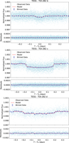 |
Fig. 1 From top to bottom: folded TESS transit light curves of TOI-282 b, c, and d. The photometric data points are plotted with light-blue circles. The dark blue circles mark the 30-minute binned data points. The best-fitting models are over-plotted with red curves. The lower panels display the residuals of the models. |
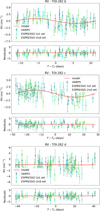 |
Fig. 2 From top to bottom: folded RV stellar signals induced by TOI-282 b, c, and d, and best-fitting RV models (red curve). The data includes 37 HARPS spectra (blue circular points) and 8 + 36 ESPRESSO spectra (cyan triangular and green square points, respectively). The lower panels show the residuals to the models. |
6 Dynamical modelling
6.1 Transit timing variation and RV dynamical analysis
In multi-planet systems, mutual gravitational interactions between the planets lead to small deviations from Keplerian motions, producing observable variations in the timing of transits (Agol et al. 2005; Holman & Murray 2005). By tracking these deviations from a linear ephemeris, known as transit timing variations (TTVs), we can probe the system’s dynamics, detect non-transiting companions, and constrain planetary masses and orbital parameters. Furthermore, by combining RV measurements with TTVs, we can break the intrinsic degeneracies of each method, enabling a more complete and robust characterisation of the system.
We found that TOI-282b displays no significant TTVs (Fig. 3), in agreement with the findings of D22. TOI-282 c and d show strong TTVs with a peak-to-peak amplitude of ~4 and ~8 hours, respectively (Fig. 4). Although the Doppler reflex motion induced by planet d remains undetected in our RV time series, its TTVs anti-correlate with those of TOI-282 c (Fig. 4), suggesting a possible resonant configuration with planet c. To measure the mass of TOI-282 d, we performed a N-body integration dynamical analysis of the planetary system, simultaneously modelling TTVs (Tables B.4, B.5, and B.6) along with the detrended RVs (Sect. 4, and Tables B.1 and B.3). For TOI-282 b, we excluded 9 transit timings, as their uncertainties σT ≳ 4 hours. The analysis was conducted using TRAnsits and Dynamics of Exoplanetary Systems (TRADES, Borsato et al. 2014, 2019, 2021)9, a Fortran-Python hybrid code that simultaneously fits transit timings and RV measurements, while self-consistently integrating planetary orbits. To cover the observational baseline, we performed a dynamical integration spanning 2410 days, initialised at the reference epoch 2 458 337 BJDTDB.
For each planet we fitted the orbital period P, the planet-to-star mass ratios Mp/M⋆, the eccentricities e, the argument of peri-centre of the planetary orbit ωp, and mean longitude λ10. To mitigate biases, we adopted the ![Mathematical equation: $\[\left(\sqrt{e} ~\cos~ \omega_{p}, \sqrt{e} ~\sin~ \omega_{p}\right)\]$](/articles/aa/full_html/2025/12/aa56791-25/aa56791-25-eq61.png) parametrisation, rather than modelling e and ωp separately. Planetary radii Rp, stellar radius R⋆ and mass M⋆, and orbital inclinations i were fixed to the values listed in Tables 1 and 2. The longitude of the ascending node was fixed to Ω = 180° for all planets. We adopted uniform priors for all the fitted parameters (Table B.7). We also fitted an RV jitter term (σjitter), by adopting log2 σjitter as a step parameter.
parametrisation, rather than modelling e and ωp separately. Planetary radii Rp, stellar radius R⋆ and mass M⋆, and orbital inclinations i were fixed to the values listed in Tables 1 and 2. The longitude of the ascending node was fixed to Ω = 180° for all planets. We adopted uniform priors for all the fitted parameters (Table B.7). We also fitted an RV jitter term (σjitter), by adopting log2 σjitter as a step parameter.
The initial exploration of the parameter space was conducted via the PyDE11 differential evolution algorithm (Storn & Price 1997; Parviainen et al. 2016), using a population size of 120 for 60 000 iterations. The solutions were then used as initial parameters for emcee (Foreman-Mackey et al. 2013), where 120 walkers explored the parameter space for 400 000 steps, approximately six times the number of free parameters in our model. Following Nascimbeni et al. (2024), our emcee sampler combined the differential evolution proposal (80% walkers; Nelson et al. 2014) with the snooker variant (20% walkers; ter Braak & Vrugt 2008). After confirming chain convergence via Geweke (Geweke 1991), Gelman-Rubin (Gelman & Rubin 1992), autocorrelation (Goodman & Weare 2010), and visual diagnostics, we discarded 100 000 steps as burn-in and applied a thinning factor of 100. Parameter uncertainties were quantified using the 68.3% highest density intervals (HDIs) of the marginalised posteriors. Inferred values correspond to the maximum a posteriori (MAP) estimates derived from the posterior distributions.
The parameter estimates and their uncertainties, along with the adopted priors, are listed in Table B.7, whereas the observed minus calculated (O–C) diagrams for TOI-282 b, c, and d are shown in Figs. 3 and 4. The anti-correlation patterns follow the model prediction made by D22. Our dynamical analysis allowed us to retrieve the orbital configuration of TOI-282b,c, and d. This approach provides the masses of the two innermost planets Mb = ![Mathematical equation: $\[6.7_{-0.8}^{+1.7}\]$](/articles/aa/full_html/2025/12/aa56791-25/aa56791-25-eq62.png) and Mc =
and Mc = ![Mathematical equation: $\[10_{-2}^{+1}\]$](/articles/aa/full_html/2025/12/aa56791-25/aa56791-25-eq63.png) , which are in very good agreement with the MCMCI-derived ones (Table 2). Moreover, we obtained a robust mass determination for TOI-282d of Md =
, which are in very good agreement with the MCMCI-derived ones (Table 2). Moreover, we obtained a robust mass determination for TOI-282d of Md = ![Mathematical equation: $\[5.8_{-1.1}^{+0.9}\]$](/articles/aa/full_html/2025/12/aa56791-25/aa56791-25-eq64.png) M⊕ (~15-20% relative precision). When combined with the radius of Rd = 3.11 ± 0.15 R⊕, the mass of TOI-282 d implies a mean density of ρd =
M⊕ (~15-20% relative precision). When combined with the radius of Rd = 3.11 ± 0.15 R⊕, the mass of TOI-282 d implies a mean density of ρd = ![Mathematical equation: $\[1.1_{-0.2}^{+0.3}\]$](/articles/aa/full_html/2025/12/aa56791-25/aa56791-25-eq65.png) g cm−3 (~25% relative precision). We acknowledge that, while the available TTV and RV data provide a relatively precise mass determination, the O–C diagrams (Fig. 4) partially cover the ~9000-day TTV super-period (Eq. (5) from Lithwick et al. 2012) of the near 3:2 pair. To accurately measure the planetary mass via TTV, a better sampling of the entire super-period is needed to reduce possible systematic uncertainties and degeneracies between eccentricity and mass solutions.
g cm−3 (~25% relative precision). We acknowledge that, while the available TTV and RV data provide a relatively precise mass determination, the O–C diagrams (Fig. 4) partially cover the ~9000-day TTV super-period (Eq. (5) from Lithwick et al. 2012) of the near 3:2 pair. To accurately measure the planetary mass via TTV, a better sampling of the entire super-period is needed to reduce possible systematic uncertainties and degeneracies between eccentricity and mass solutions.
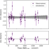 |
Fig. 3 Observed minus calculated (O–C) TTV diagram for TOI-282b, showing TTV as a function of time. The shaded regions represent the 1,2, and 3σ confidence interval derived from the posterior distributions of the model parameters of our dynamical analysis. |
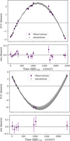 |
Fig. 4 Observed minus calculated (O–C) TTV diagrams for TOI-282 c (upper panel) and TOI-282d (lower panel), showing TTV as a function of time. The shaded regions represent the 1,2, and 3σ confidence interval derived from the posterior distributions of the model parameters of our dynamical analysis. Both planets exhibit anti-correlated TTV exceeding the transit time uncertainties. |
6.2 Stability analysis
As an additional check in our dynamical analysis, TRADES assesses the system’s Hill stability using the AMD-Hill criterion (Eq. (26); Petit et al. 2018), which is based on the angular momentum deficit (AMD; Laskar 1997, 2000; Laskar & Petit 2017). We find that the entire posterior distribution satisfies the AMD-Hill stability criterion, indicating long-term dynamical stability. To further evaluate the stability and potential chaotic behaviour of the posterior solutions, accounting for planet-planet interactions, mean-motion resonances, and possible planetary ejections, we performed N-body integrations with rebound (Rein & Liu 2012; Rein & Tamayo 2016). Specifically, we employed the mean exponential growth factor of nearby orbits (MEGNO; ⟨Y⟩) chaos indicator (Cincotta & Simó 2000; Cincotta et al. 2003), as implemented in rebound. We defined a dynamically stable planetary configuration as satisfying ⟨Y⟩ ≤ 2.5 (Cincotta & Simó 2000), with planetary ejection occurring if any body’s semi-major axis exceeds 100 ad. Using the symplectic integrator WHFast (Rein & Tamayo 2016), we propagated orbits for 100 kyr with a time-step equal to 10% of planet b’s orbital period (tstep ≈ 0.1 Pb). For MAP solution within the highest density interval (HDI), we found ⟨Y⟩ < 2.5, indicating a strongly stable dynamics. To assess broader posterior solutions, we ran the integration for 500 randomly selected posteriors. We found that ~92% of the simulations were stable.
We also simulated the evolution of the system for 105 years, adopting a fourth-order Runge-Kutta (RK4) algorithm (Runge 1895). For each planet, we studied the evolution of the semimajor axis A, eccentricity e, argument of peri-centre ωp, inclination i, and longitude of ascending node Ω. Our results are shown in Fig. 5 for two different time intervals, with Fig. 5a showing the 105−year evolution and Fig. 5b covering the first 104 years. We found that:
The semi-major axes (a) do not change significantly over time, with relative variations never exceeding 0.1% (Fig. 5a, first panel).
The eccentricities (e) of TOI-282 c and TOI-282 d oscillate with a period of about 280 years, reaching a maximum value of ~0.01 (Fig. 5a, second panel, and Fig. 5b, first panel). The oscillations have a super-period that matches the TOI-282b eccentricity evolution period of about 10500 years.
A peri-centre precession period of ~7150 years for TOI-282 b, and ~270 years for both planets c and d (Fig. 5a, third panel, and Fig. 5b, second panel). Along with the precession motion, we also found that the peri-centre angle of TOI-282b (ωb) oscillates with a semi-amplitude of 30 degrees in quadrature with the evolution of its eccentricity (eb).
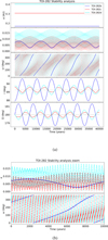
Fig. 5 Simulated evolution of the orbital parameters over 105 years. Figure b shows a zoom over the first 104 years on the eccentricity and argument of peri-centre plots. The colours blue, red, cyan refer respectively to planets TOI-282b, TOI-282c, TOI-282d.
The orbital planes display a precession motion around their mean value, with the inclinations (i) and corresponding longitudes of the ascending node (Ω) evolving in quadrature (Fig. 5a, fourth and fifth panels). The primary period of about 6890 years is given by the relative (anti-phased) oscillation between the angular momentum of TOI-282b and the total angular momentum of TOI-282 c and TOI-282 d. The orbital planes of the two resonant outer planets also oscillate in anti-phase around their average value with a period of about 1960 years and a semi-amplitude of ~0.1°.
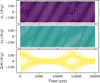 |
Fig. 6 Resonant angle evolution for TOI-282 c and d, for the MAP solutions. The two upper panels show the evolution of the critical angles for the 3:2 resonance (ϕc and ϕd); the lower panel shows the difference between the longitudes of pericentre (Δϖ). |
6.3 Resonant angles evolution
While period ratios near low-integer fractions may suggest proximity to a mean motion resonance, they do not definitively confirm it. Following Lithwick et al. (2012), we computed the so-called ‘resonance offset’, i.e. the deviation from the exact commensurability defined as Δ = (Pout/Pin)/(q/p) − 1, where q = 3 and p = 2 for a 3:2 configuration. The resonance offset for TOI-282 c and d is Δ ≈ 0.0035, which agrees to the values found by N-body and hydrodynamical simulations (e.g Silburt & Rein 2015; Ramos et al. 2017), and may indicate that the planets are in a resonance configuration, with librating resonant ‘arguments’. To uniquely assess if two outer planets are actually in an MMR, one must examine whether the critical resonant angles librate (oscillate around a fixed value) or circulate (continuously increase/decrease). Exact two-body first-order resonance requires libration within ±180° of one or both of: ϕ1 = qλ1 − (q + 1)λ2 + ϖ1, ϕ2 = qλ1 − (q + 1)λ2 + ϖ2. To investigate the resonant state of TOI-282 c and TOI-282 d, we integrated the MAP solutions using the N-body code rebound (Rein & Liu 2012) and the symplectic integrator WHFast (Rein & Tamayo 2016), for a total of 20 000 years. We computed the evolution of the resonant angles, defined as:
![Mathematical equation: $\[\begin{aligned}& \phi_c=2 \lambda_c-3 \lambda_d+\varpi_c, \\& \phi_d=2 \lambda_c-3 \lambda_d+\varpi_d,\end{aligned}\]$](/articles/aa/full_html/2025/12/aa56791-25/aa56791-25-eq66.png) (2)
(2)
where ϖ = ω + Ω denotes the longitude of peri-centre. As shown in Figure 6, which also includes Δϖ ≡ ϖc − ϖd, both angles circulate, indicating the system is not locked in a stable 3:2 resonance.
7 The planetary system TOI-282
In agreement with D22, our results confirm that the F8 dwarf star TOI-282 hosts two sub-Neptunes (TOI-282 b and d) and one Neptune-sized planet (TOI-282 c), adopting the notation proposed by Kopparapu et al. (2018). With P < 100 days and period ratios Pc/Pb and Pd/Pc < 5, TOI-282 b, c, and d can be considered ‘inner’ planets with no significant gaps in the orbital periods (Howe et al. 2025). Following Mishra et al. (2023), given their masses and radii, the three planets can be defined as ‘similar’. For instance, their masses imply a coefficient of similarity of CS(M) = 0.008 and a coefficient of variation of CV(M) = 0.2, with the conditions of ’similarity’ for TOI-282 being |CS (M)| ≤ 0.2 and CV(M) ≤ 0.7 (Mishra et al. 2023). This allows us to define the architecture of TOI-282 as a close-in “right-in-a-pod” configuration, the most common architecture among the known multi-planet systems, representing ~87% of the peas-in-a-pod systems and ~80% of all the known planetary systems with at least 3 inner planets (Howe et al. 2025). These systems offer valuable insights into the formation and evolution of planets, being primary products of planet formation. The eccentricities and mutual inclinations of the planets are usually close to zero, and their internal compositions are similar. This suggests that compact, close-in systems represent the lowest energy state accessible to a forming planetary system. The three planets orbiting TOI-282 might have formed beyond the ice line and then migrated inward, reaching their current configuration through energy dissipation mechanisms. The similarity between the three planets would be a consequence of the same formation mechanism (Weiss et al. 2022).
We compared the positions of TOI-282 b, c, and d in the mass-radius (MR) diagram with those of other known exoplanets. We retrieved from the NASA Exoplanet Archive12 masses and radii for the spectroscopically confirmed transiting exoplanets as of June 2025, and selected only those planets whose mass and radius were determined with relative precisions better than 30% and 10%, respectively. We chose the most recent reference for planets with different mass and radius estimates. Figure 7 shows the MR diagram of the planets that meet our criteria, colour-coded by their equilibrium temperature when available. To gain insight into the internal compositions of the planets, we also include the theoretical internal models from Zeng et al. (2019).
TOI-282 b falls above a ‘crowded’ region of the MR diagram, in a quite degenerate parameter space, where it is difficult to obtain meaningful information on the composition of the planets. The planet could have an Earth-like rocky core (32.5% Fe + 67.5% MgSiO3), representing 99% of its mass, surrounded by a 1% H2 envelope13. Alternatively, TOI-282 b could be composed of a 1:1 mixture of H2O ice and rocks, making it a new member of the so-called population of ‘water worlds’ (Léger et al. 2004; Rogers 2015; Mousis et al. 2020; Dorn & Lichtenberg 2021; Luque & Pallé 2022), with ~0.3% molecular hydrogen in its atmospheric envelope. From the composition of TOI-282 b, it would be possible to gain insight into its evolution and formation. Water worlds are believed to have formed beyond the ice line and then migrated towards the inner regions of the system (Raymond et al. 2018; Bitsch et al. 2019; Izidoro et al. 2022). On the other hand, Earth-like rocky planets are expected to be formed in situ, in the inner regions of the protoplanetary disc, and, in the absence of photo-evaporation processes, would retain their primordial atmosphere without being substantially enriched in volatiles (Ikoma & Hori 2012; Lee et al. 2014; Lee & Chiang 2016). Due to the degeneracy, it is worth stressing that the super-imposed theoretical models are not intended to give a definitive prediction on the composition of the planet, but rather a preliminary assessment of its possible internal structure (e.g. Rogers & Seager 2010; Lopez & Fortney 2014; Dorn et al. 2015, 2017; Otegi et al. 2020).
With its low mean density (ρc = 0.7 ± 0.2 g cm−3), TOI-282 c appears to be isolated in the MR diagram (Fig. 7). Once again, theoretical models are found to be degenerate in this region of the parameter space. In fact, TOI-282 c might either have an Earth-like rocky core or might be composed of a 1:1 mixture of ice and rocks, with 5% molecular hydrogen in its atmosphere. The outer transiting planet, TOI-282 d, also seems to be relatively isolated in the MR diagram (Fig. 7). According to Zeng et al. (2019), it may also be a water world with 2% molecular hydrogen in its envelope. If the three planets around TOI-282 were water worlds, they would follow the recent findings of Venturini et al. (2024), where planets orbiting stars in the mass range 0.1 ≤ M⋆ ≤ 1.5 M⊙ tend to be larger water worlds, rather than smaller rocky planets.
The low mean density of TOI-282 c and d, along with their relatively isolated positions in the MR diagram, could be linked to their nearly resonant state (see Section 6.3; Leleu et al. 2024). Following Lee & Chiang (2016), sub-Neptunes can form further out in the protoplanetary disc (in gas-poor regions), and enter an MMR state because of the subsequent inward migration. Alternatively, according to the “breaking the chains” model (Bean et al. 2021), sub-Neptunes in (close) MMR state may form in resonant chains due to the migration of planets in the protoplanetary discs and the positive torque at the inner edge of the disc (e.g. Goldreich & Tremaine 1979; Weidenschilling & Davis 1985; Masset et al. 2006; Terquem & Papaloizou 2007). Instead, instabilities in the chains might lead to impacts, which may eject parts of the planet’s primordial atmosphere (Biersteker & Schlichting 2019) and result in denser non-resonant objects, which could explain the nature of TOI-282b. The coplanarity of TOI-282c and d (Δic,d = 0.2 ± 0.2°) strengthens this possibility, as planets in resonant chains tend to be coplanar (Agol et al. 2021; Leleu et al. 2021). At the same time, planet-planet scatterings are expected to increase the mutual inclinations (Δib,c = 1.7 ± 0.2° and Δib,d = 1.8 ± 0.2°).
The three planets in the TOI-282 system span a relatively small range of radii (2.7–4.1 R⊕) and masses (6.2–9.2 M⊕). They are all located above the so-called radius valley – a dearth of small planets around ~1.5–2.0 R⊕ (see Fig. 4 in Owen & Wu 2017) – and their relatively large radii can be explained by the presence of a thick atmosphere. This holds particularly for the two outermost transiting planets, as planets with radii R ≳ 3 R⊕ are expected to have H/He in their atmosphere (Jin & Mordasini 2018), and their long orbital periods (P > 50 days) make a major mass loss due to photo-evaporation unlikely (Gupta & Schlichting 2020). To explore the feasibility of atmospheric characterisation of the system, we determined for each planet the transmission and emission spectroscopy metrics (TSMs and ESMs; Kempton et al. 2018). Starting from the closest planet to the star and moving further out, the TSMs are ~39, 71, and 42, respectively, while the ESMs are ~1.6, 1.8, and 0.7. The ESM is proportional to the expected S/N of a JWST planet occultation detection. We derived emission metrics values which are well below the recommended threshold (ESM = 7.5), suggesting that it will probably not be possible to detect the occultations of the planets, mainly due to their low equilibrium temperatures (Table 2). On the other hand, even though TOI-282 b, c, and d do not seem to be high-priority targets for transmission spectroscopy14, the bright host star in combination with the planets’ radii, masses, and equilibrium temperatures led to acceptable metrics for atmospheric characterisation. Particularly, the three planets have a TSM higher than the lowest value of a top candidate in the radius bin of interest presented in Izidoro et al. (2022). For instance, when compared to ~1500 transiting exoplanets with known masses, we derived a quantile of 0.56, 0.39, and 0.54, respectively, making their atmospheric characterisation still feasible.
The TOI-282 system may be amenable to atmospheric characterisation via infrared high-resolution spectroscopy (HRS) with the ESO Extremely Large Telescope (ELT). Using Teq in Table 2 (zero albedo, full recirculation), the signal corresponding to 5 scale heights – typical for strong molecular lines in the near infrared – ranges from 33 to 60 ppm. Given the relatively bright host star (Table 1), with the ANDESatELT spectrograph (Marconi et al. 2024), it might be possible to detect TOI-282 c and d with one full transit (8–10 hours), while planet b would require 2–3 transits. Such observations would reveal the detailed chemical composition of the exoplanets, including potential N-bearing species associated with photochemical processes and the overall planet metallicity, the latter useful to break the degeneracy between interiors and envelopes.
With HRS, the ESM is not necessarily a good emission metric as the signal is driven by line contrast rather than continuum contrast. Using continuum contrast as a best-case scenario, ANDES would not be able to detect any of the planets easily. Even for TOI-282b, the flux ratio ranges between 10−10 at 1 μm and 10−7 at 1.8 μm, and it is 2–3 orders of magnitude worse for the cooler planets c and d. Such contrast ratios are beyond reach in spatially unresolved HRS.
Nevertheless, in the METISatELT bandpass (3–5 μm; Brandl et al. 2021), planet b would have a photospheric contrast of a few parts per million per line, which is about a factor of 10 smaller than typical 3σ contrasts routinely achieved by current photon-limited HRS on 8–10-metre class telescopes. Considering the gain in collective area from the ELT, it may be possible to detect TOI-282b in 10–20 hours on sky, achievable in 2–3 scheduled nights of observations since HRS can observe both before and after a secondary eclipse.
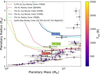 |
Fig. 7 Mass-radius diagram showing the position of TOI-282b (Teq = 867 ± 16 K), TOI-282 c (Teq = 643 ± 12 K), and TOI-282 d (Teq = 561 ± 11 K) with respect to the transiting planets whose masses and radii are known with a precision better than 30% and 10%, respectively (circles). The coloured lines show the theoretical models from Zeng et al. (2019). |
8 Conclusions
TOI-282 is a late F-type bright (V=9.38) dwarf star, which hosts 3 long-period transiting small planets, with the outer two being close to a 3:2 MMR. The system was discovered and validated by D22, combining TESS space-based photometry with ground-based transit observations. We analysed 38 TESS sectors (15 more than those presented in D22), increasing the time baseline by nearly 3 years. We found that TOI-282b,c, and d have radii of Rb = 2.69 ± 0.23 R⊕, Rc = ![Mathematical equation: $\[4.13_{-0.14}^{+0.16}\]$](/articles/aa/full_html/2025/12/aa56791-25/aa56791-25-eq67.png) R⊕, and Rd = 3.11 ± 0.15 R⊕, with a relative precision of 9%, 4%, and 5%, respectively.
R⊕, and Rd = 3.11 ± 0.15 R⊕, with a relative precision of 9%, 4%, and 5%, respectively.
We performed an intensive RV follow-up of the star, securing 37 HARPS and 44 ESPRESSO high-precision Doppler measurements, which we jointly model with the TESS transit LCs. We obtained a solid detection of the Doppler reflex motion induced by the two innermost planets (~4 and 5σ level) and measured a mass of Mb = 6.2 ± 1.6 M⊕ and Mc = 9.2 ± 2.0 M⊕ for TOI-282 b and c, respectively. Although the outer planet (TOI-282 d) remains undetected in our RV time series, we determined its mass by performing a dynamical analysis of the system, leveraging the significant anti-correlated TTVs exhibited by TOI-282 c and TOI-282 d. We found that TOI-282 d has a mass of Md = ![Mathematical equation: $\[5.8_{-1.1}^{+0.9}\]$](/articles/aa/full_html/2025/12/aa56791-25/aa56791-25-eq68.png) M⊕ (~15–20% relative precision). The three planets have mean densities of ρb =
M⊕ (~15–20% relative precision). The three planets have mean densities of ρb = ![Mathematical equation: $\[1.8_{-0.6}^{+0.7}\]$](/articles/aa/full_html/2025/12/aa56791-25/aa56791-25-eq69.png) g cm−3, ρc = 0.7 ± 0.2 g cm−3, and ρd =
g cm−3, ρc = 0.7 ± 0.2 g cm−3, and ρd = ![Mathematical equation: $\[1.1_{-0.2}^{+0.3}\]$](/articles/aa/full_html/2025/12/aa56791-25/aa56791-25-eq70.png) g cm−3, which implies a relative precision of ~36%, 29%, and 25%, respectively.
g cm−3, which implies a relative precision of ~36%, 29%, and 25%, respectively.
We also investigated the long-term dynamical evolution of the system to study the behaviour of the resonant angles associated with the two outer planets and the stability of the system’s orbital architecture. According to our simulations, while the system remains dynamically stable, the outer planet pair lies near, but does not maintain, a 3:2 MMR. We then placed the planets in an MR diagram to gain insight into their internal composition. By comparing the positions of the three planets on the MR diagram with internal structure models by Zeng et al. (2019), we found that TOI-282 b and c might either be water worlds or have a rocky composition, while TOI-282 d could be a water world.
Further investigation of the system might break the internal composition degeneracy and provide insights into the nature and evolution of the three small planets transiting TOI-282. Future transmission spectroscopic observations with JWST and ELT are, in theory, feasible, as suggested by the derived metrics for atmospheric signals, and TOI-282 could be a high-priority target. TESS will observe the system from sector 93 (July 2025) through sector 98 (January 2026), providing an improved coverage of the TTV super-period.
Data availability
Tables B.1, B.2, and B.3 are available at the CDS via https://cdsarc.cds.unistra.fr/viz-bin/cat/J/A+A/704/A41.
Acknowledgements
We thank the referee for the comments and suggestions that helped us to improve the quality of our paper. We express our deepest gratitude to the ESO staff members for their unique support during the observations. A.Ba and D.Ga. gratefully acknowledge the funding from the Physics Department of the University of Turin. We thank Domenico Nardiello, David Rapetti, and Jon Jenkins for their precious efforts in reprocessing the TESS light curves to recover the transit photometry that falls within the gaps of the PDCSAP time series. We acknowledge financial support from the Agencia Estatal de Investigación of the Ministerio de Ciencia e Innovación MCIN/AEI/10.13039/501100011033 and the ERDF “A way of making Europe” through project PID2021-125627OBC32, and from the Centre of Excellence “Severo Ochoa” award to the Instituto de Astrofisica de Canarias. P.Le. acknowledges that this publication was produced while attending the PhD program in Space Science and Technology at the University of Trento, Cycle XXXVIII, with the support of a scholarship co-financed by the Ministerial Decree no. 351 of 9th April 2022, based on the NRRP – funded by the European Union – NextGenerationEU – Mission 4 “Education and Research”, Component 2 “From Research to Business”, Investment 3.3 – CUP E63C22001340001.
References
- Agol, E., Steffen, J., Sari, R., & Clarkson, W. 2005, MNRAS, 359, 567 [Google Scholar]
- Agol, E., Dorn, C., Grimm, S. L., et al. 2021, Planet. Sci. J., 2, 1 [NASA ADS] [CrossRef] [Google Scholar]
- Anglada-Escudé, G., & Butler, R. P. 2012, ApJS, 200, 15 [Google Scholar]
- Bai, J., & Perron, P. 2003, J. Appl. Econom., 18, 1 [CrossRef] [Google Scholar]
- Baranne, A., Queloz, D., Mayor, M., et al. 1996, A&AS, 119, 373 [NASA ADS] [CrossRef] [EDP Sciences] [Google Scholar]
- Batalha, N. M., Rowe, J. F., Bryson, S. T., et al. 2013, ApJSS, 204, 24 [NASA ADS] [CrossRef] [Google Scholar]
- Bean, J. L., Raymond, S. N., & Owen, J. E. 2021, J. Geophys. Res. (Planets), 126, e06639 [NASA ADS] [Google Scholar]
- Biersteker, J. B., & Schlichting, H. E. 2019, MNRAS, 485, 4454 [NASA ADS] [CrossRef] [Google Scholar]
- Bitsch, B., Raymond, S. N., & Izidoro, A. 2019, A&A, 624, A109 [NASA ADS] [CrossRef] [EDP Sciences] [Google Scholar]
- Boisse, I., Bouchy, F., Hébrard, G., et al. 2011, A&A, 528, A4 [NASA ADS] [CrossRef] [EDP Sciences] [Google Scholar]
- Bonfanti, A., & Gillon, M. 2020, A&A, 635, A6 [NASA ADS] [CrossRef] [EDP Sciences] [Google Scholar]
- Bonfanti, A., Ortolani, S., Piotto, G., & Nascimbeni, V. 2015, A&A, 575, A18 [NASA ADS] [CrossRef] [EDP Sciences] [Google Scholar]
- Bonfanti, A., Ortolani, S., & Nascimbeni, V. 2016, A&A, 585, A5 [NASA ADS] [CrossRef] [EDP Sciences] [Google Scholar]
- Bonfanti, A., Delrez, L., Hooton, M. J., et al. 2021, A&A, 646, A157 [EDP Sciences] [Google Scholar]
- Bonfanti, A., Gandolfi, D., Egger, J. A., et al. 2023, A&A, 671, L8 [NASA ADS] [CrossRef] [EDP Sciences] [Google Scholar]
- Bonfanti, A., Amateis, I., Gandolfi, D., et al. 2025, A&A, 693, A90 [NASA ADS] [CrossRef] [EDP Sciences] [Google Scholar]
- Borsato, L., Marzari, F., Nascimbeni, V., et al. 2014, A&A, 571, A38 [NASA ADS] [CrossRef] [EDP Sciences] [Google Scholar]
- Borsato, L., Malavolta, L., Piotto, G., et al. 2019, MNRAS, 484, 3233 [NASA ADS] [CrossRef] [Google Scholar]
- Borsato, L., Piotto, G., Gandolfi, D., et al. 2021, MNRAS, 506, 3810 [NASA ADS] [CrossRef] [Google Scholar]
- Brandl, B., Bettonvil, F., van Boekel, R., et al. 2021, The Messenger, 182, 22 [NASA ADS] [Google Scholar]
- Bruntt, H., De Cat, P., & Aerts, C. 2008, A&A, 478, 487 [NASA ADS] [CrossRef] [EDP Sciences] [Google Scholar]
- Castelli, F., & Hubrig, S. 2004, A&A, 425, 263 [NASA ADS] [CrossRef] [EDP Sciences] [Google Scholar]
- Cincotta, P. M., Giordano, C. M., & Simó, C. 2003, Physica D Nonlinear Phenomena, 182, 151 [NASA ADS] [CrossRef] [Google Scholar]
- Cincotta, P. M., & Simó, C. 2000, A&AS, 147, 205 [NASA ADS] [CrossRef] [EDP Sciences] [Google Scholar]
- Cutri, R. M., Skrutskie, M. F., van Dyk, S., et al. 2003, 2MASS All Sky Catalog of point sources. (University of Massachusetts and Infrared Processing and Analysis Center (IPAC/California Institute of Technology)) [Google Scholar]
- Dorn, C., & Lichtenberg, T. 2021, ApJ, 922, L4 [NASA ADS] [CrossRef] [Google Scholar]
- Dorn, C., Khan, A., Heng, K., et al. 2015, A&A, 577, A83 [NASA ADS] [CrossRef] [EDP Sciences] [Google Scholar]
- Dorn, C., Venturini, J., Khan, A., et al. 2017, A&A, 597, A37 [NASA ADS] [CrossRef] [EDP Sciences] [Google Scholar]
- Doyle, A. P., Davies, G. R., Smalley, B., Chaplin, W. J., & Elsworth, Y. 2014, MNRAS, 444, 3592 [Google Scholar]
- Dransfield, G., Triaud, A. H. M. J., Guillot, T., et al. 2022, MNRAS, 515, 1328 [NASA ADS] [CrossRef] [Google Scholar]
- Dumusque, X. 2018, A&A, 620, A47 [NASA ADS] [CrossRef] [EDP Sciences] [Google Scholar]
- Dumusque, X., Santos, N. C., Udry, S., Lovis, C., & Bonfils, X. 2011, A&A, 527, A82 [NASA ADS] [CrossRef] [EDP Sciences] [Google Scholar]
- Eastman, J., Siverd, R., & Gaudi, B. S. 2010, PASP, 122, 935 [Google Scholar]
- Espinoza, N., & Jordán, A. 2015, MNRAS, 450, 1879 [Google Scholar]
- Faria, J. P., Adibekyan, V., Amazo-Gómez, E. M., et al. 2020, A&A, 635, A13 [NASA ADS] [CrossRef] [EDP Sciences] [Google Scholar]
- Figueira, P., Santos, N. C., Pepe, F., Lovis, C., & Nardetto, N. 2013, A&A, 557, A93 [NASA ADS] [CrossRef] [EDP Sciences] [Google Scholar]
- Foreman-Mackey, D., Hogg, D. W., Lang, D., & Goodman, J. 2013, PASP, 125, 306 [Google Scholar]
- Fridlund, M., Georgieva, I. Y., Bonfanti, A., et al. 2024, A&A, 684, A12 [NASA ADS] [CrossRef] [EDP Sciences] [Google Scholar]
- Gaia Collaboration (Vallenari, A., et al.) 2023, A&A, 674, A1 [NASA ADS] [CrossRef] [EDP Sciences] [Google Scholar]
- Gandolfi, D., Barragán, O., Hatzes, A. P., et al. 2017, AJ, 154, 123 [NASA ADS] [CrossRef] [Google Scholar]
- Gandolfi, D., Alnajjarine, A., Serrano, L. M., et al. 2025, https://doi.org/10.1051/0004-6361/202554631 [Google Scholar]
- Gardner, J. P., Mather, J. C., Clampin, M., et al. 2006, Space Sci. Rev., 123, 485 [Google Scholar]
- Gelman, A., & Rubin, D. B. 1992, Statist. Sci., 7, 457 [NASA ADS] [Google Scholar]
- Geweke, J. F. 1991, Evaluating the accuracy of sampling-based approaches to the calculation of posterior moments, Staff Report 148, Federal Reserve Bank of Minneapolis [Google Scholar]
- Giacobbe, P., Brogi, M., Gandhi, S., et al. 2021, Nature, 592, 205 [NASA ADS] [CrossRef] [Google Scholar]
- Goffo, E., Gandolfi, D., Egger, J. A., et al. 2023, ApJ, 955, L3 [NASA ADS] [CrossRef] [Google Scholar]
- Goldreich, P., & Tremaine, S. 1979, ApJ, 233, 857 [Google Scholar]
- Goodman, J., & Weare, J. 2010, Commun. Appl. Math. Computat. Sci., 5, 65 [Google Scholar]
- Gupta, A., & Schlichting, H. E. 2020, MNRAS, 493, 792 [Google Scholar]
- Hatzes, A. P. 1996, PASP, 108, 839 [NASA ADS] [CrossRef] [Google Scholar]
- Hatzes, A. P., Dvorak, R., Wuchterl, G., et al. 2010, A&A, 520, A93 [NASA ADS] [CrossRef] [EDP Sciences] [Google Scholar]
- Haywood, R. D., Collier Cameron, A., Queloz, D., et al. 2014, MNRAS, 443, 2517 [Google Scholar]
- Høg, E., Fabricius, C., Makarov, V. V., et al. 2000, A&A, 355, L27 [Google Scholar]
- Holman, M. J., & Murray, N. W. 2005, Science, 307, 1288 [Google Scholar]
- Holman, M. J., Winn, J. N., Latham, D. W., et al. 2006, ApJ, 652, 1715 [NASA ADS] [CrossRef] [Google Scholar]
- Howe, A. R., Becker, J. C., Stark, C. C., & Adams, F. C. 2025, AJ, 169, 149 [Google Scholar]
- Husser, T. O., Wende-von Berg, S., Dreizler, S., et al. 2013, A&A, 553, A6 [NASA ADS] [CrossRef] [EDP Sciences] [Google Scholar]
- Ikoma, M., & Hori, Y. 2012, ApJ, 753, 66 [NASA ADS] [CrossRef] [Google Scholar]
- Izidoro, A., Schlichting, H. E., Isella, A., et al. 2022, ApJ, 939, L19 [NASA ADS] [CrossRef] [Google Scholar]
- Jenkins, J. M., Twicken, J. D., McCauliff, S., et al. 2016, SPIE Conf. Ser.,. 9913, 99133E [Google Scholar]
- Jin, S., & Mordasini, C. 2018, ApJ, 853, 163 [Google Scholar]
- Kass, R. E., & Raftery, A. E. 1995, J. Am. Statist. Assoc., 90, 773 [CrossRef] [Google Scholar]
- Kempton, E. M. R., Bean, J. L., Louie, D. R., et al. 2018, PASP, 130, 114401 [Google Scholar]
- Kempton, E. M. R., & Knutson, H. A. 2024, Transiting Exoplanet Atmospheres in the Era of JWST [Google Scholar]
- Kopparapu, R. K., Hébrard, E., Belikov, R., et al. 2018, ApJ, 856, 122 [NASA ADS] [CrossRef] [Google Scholar]
- Kuerster, M., Schmitt, J. H. M. M., Cutispoto, G., & Dennerl, K. 1997, A&A, 320, 831 [Google Scholar]
- Kurucz, R. L. 1993, VizieR Online Data Catalog: Model Atmospheres (Kurucz, 1979), VizieR On-line Data Catalog: VI/39. Originally published in: 1979ApJS...40....1K [Google Scholar]
- Kurucz, R. L. 2013, ATLAS12: Opacity sampling model atmosphere program, Astrophysics Source Code Library [record ascl:1303.024] [Google Scholar]
- Laskar, J. 1997, A&A, 317, L75 [NASA ADS] [Google Scholar]
- Laskar, J. 2000, Phys. Rev. Lett., 84, 3240 [Google Scholar]
- Laskar, J., & Petit, A. C. 2017, A&A, 605, A72 [NASA ADS] [CrossRef] [EDP Sciences] [Google Scholar]
- Lee, E. J., & Chiang, E. 2016, ApJ, 817, 90 [Google Scholar]
- Lee, E. J., Chiang, E., & Ormel, C. W. 2014, ApJ, 797, 95 [Google Scholar]
- Leleu, A., Alibert, Y., Hara, N. C., et al. 2021, A&A, 649, A26 [NASA ADS] [CrossRef] [EDP Sciences] [Google Scholar]
- Leleu, A., Delisle, J.-B., Burn, R., et al. 2024, A&A, 687, L1 [NASA ADS] [CrossRef] [EDP Sciences] [Google Scholar]
- Lindegren, L., Bastian, U., Biermann, M., et al. 2021, A&A, 649, A4 [EDP Sciences] [Google Scholar]
- Lithwick, Y., Xie, J., & Wu, Y. 2012, ApJ, 761, 122 [Google Scholar]
- Lopez, E. D., & Fortney, J. J. 2014, ApJ, 792, 1 [Google Scholar]
- Lovis, C., & Pepe, F. 2007, A&A, 468, 1115 [NASA ADS] [CrossRef] [EDP Sciences] [Google Scholar]
- Luque, R., & Pallé, E. 2022, Science, 377, 1211 [NASA ADS] [CrossRef] [Google Scholar]
- Luque, R., Osborn, H. P., Leleu, A., et al. 2023, Nature, 623, 932 [NASA ADS] [CrossRef] [Google Scholar]
- Léger, A., Selsis, F., Sotin, C., et al. 2004, Icarus, 169, 499 [Google Scholar]
- Madhusudhan, N. 2019, ARA&A, 57, 617 [NASA ADS] [CrossRef] [Google Scholar]
- Madhusudhan, N., Agúndez, M., Moses, J. I., & Hu, Y. 2016, Space Sci. Rev., 205, 285 [Google Scholar]
- Mamajek, E. E., & Hillenbrand, L. A. 2008, ApJ, 687, 1264 [Google Scholar]
- Marconi, A., Abreu, M., Adibekyan, V., et al. 2024, SPIE Conf. Ser., 13096, 1309613 [Google Scholar]
- Marcy, G. W., Weiss, L. M., Petigura, E. A., et al. 2014, PNAS, 111, 12655 [NASA ADS] [CrossRef] [Google Scholar]
- Marigo, P., Girardi, L., Bressan, A., et al. 2017, ApJ, 835, 77 [Google Scholar]
- Masset, F. S., Morbidelli, A., Crida, A., & Ferreira, J. 2006, ApJ, 642, 478 [Google Scholar]
- Mayor, M., Pepe, F., Queloz, D., et al. 2003, The Messenger, 114, 20 [NASA ADS] [Google Scholar]
- Mishra, L., Alibert, Y., Udry, S., & Mordasini, C. 2023, A&A, 670, A68 [NASA ADS] [CrossRef] [EDP Sciences] [Google Scholar]
- Mousis, O., Deleuil, M., Aguichine, A., et al. 2020, ApJ, 896, L22 [NASA ADS] [CrossRef] [Google Scholar]
- Murdoch, K. A., Hearnshaw, J. B., & Clark, M. 1993, ApJ, 413, 349 [CrossRef] [Google Scholar]
- Nascimbeni, V., Borsato, L., Leonardi, P., et al. 2024, A&A, 690, A349 [NASA ADS] [CrossRef] [EDP Sciences] [Google Scholar]
- Nelson, B., Ford, E. B., & Payne, M. J. 2014, ApJS, 210, 11 [Google Scholar]
- Otegi, J. F., Dorn, C., Helled, R., et al. 2020, A&A, 640, A135 [NASA ADS] [CrossRef] [EDP Sciences] [Google Scholar]
- Owen, J. E., & Wu, Y. 2017, ApJ, 847, 29 [Google Scholar]
- Parviainen, H., Pallé, E., Nortmann, L., et al. 2016, A&A, 585, A114 [NASA ADS] [CrossRef] [EDP Sciences] [Google Scholar]
- Pepe, F., Mayor, M., Galland, F., et al. 2002, A&A, 388, 632 [NASA ADS] [CrossRef] [EDP Sciences] [Google Scholar]
- Pepe, F., Molaro, P., Cristiani, S., et al. 2014, Astron. Nachr., 335, 8 [Google Scholar]
- Pepe, F., Cristiani, S., Rebolo, R., et al. 2021, A&A, 645, A96 [NASA ADS] [CrossRef] [EDP Sciences] [Google Scholar]
- Persson, C. M., Fridlund, M., Barragán, O., et al. 2018, A&A, 618, A33 [NASA ADS] [CrossRef] [EDP Sciences] [Google Scholar]
- Petigura, E. A., Howard, A. W., & Marcy, G. W. 2013, PNAS, 110, 19273 [NASA ADS] [CrossRef] [Google Scholar]
- Petit, A. C., Laskar, J., & Boué, G. 2018, A&A, 617, A93 [NASA ADS] [CrossRef] [EDP Sciences] [Google Scholar]
- Petrovich, C., Muñoz, D. J., Kratter, K. M., & Malhotra, R. 2020, ApJ, 902, L5 [NASA ADS] [CrossRef] [Google Scholar]
- Piskunov, N., & Valenti, J. A. 2017, A&A, 597, A16 [NASA ADS] [CrossRef] [EDP Sciences] [Google Scholar]
- Pont, F., Zucker, S., & Queloz, D. 2006, MNRAS, 373, 231 [NASA ADS] [CrossRef] [Google Scholar]
- Queloz, D., Henry, G. W., Sivan, J. P., et al. 2001, A&A, 379, 279 [NASA ADS] [CrossRef] [EDP Sciences] [Google Scholar]
- Ramos, X. S., Charalambous, C., Benítez-Llambay, P., & Beaugé, C. 2017, A&A, 602, A101 [NASA ADS] [CrossRef] [EDP Sciences] [Google Scholar]
- Raymond, S. N., Boulet, T., Izidoro, A., Esteves, L., & Bitsch, B. 2018, MNRAS, 479, L81 [Google Scholar]
- Rein, H., & Liu, S. F. 2012, A&A, 537, A128 [NASA ADS] [CrossRef] [EDP Sciences] [Google Scholar]
- Rein, H., & Tamayo, D. 2016, MNRAS, 459, 2275 [Google Scholar]
- Richter, P. H. 1995, Telecommun. Data Acquis. Progr. Rep., 122, 107 [Google Scholar]
- Ricker, G. R., Winn, J. N., Vanderspek, R., et al. 2015, J. Astron. Telesc. Instrum. Syst., 1, 014003 [Google Scholar]
- Rogers, J. G., Schlichting, H. E., & Owen, J. E. 2023, ApJ, 947, L19 [NASA ADS] [CrossRef] [Google Scholar]
- Rogers, L. A. 2015, ApJ, 801, 41 [Google Scholar]
- Rogers, L. A., & Seager, S. 2010, ApJ, 716, 1208 [NASA ADS] [CrossRef] [Google Scholar]
- Runge, C. 1895, Math. Ann., 46, 167 [Google Scholar]
- Saar, S. H., & Donahue, R. A. 1997, ApJ, 485, 319 [Google Scholar]
- Serrano, L. M., Gandolfi, D., Mustill, A. J., et al. 2022, Nat. Astron., 6, 736 [NASA ADS] [CrossRef] [Google Scholar]
- Silburt, A., & Rein, H. 2015, MNRAS, 453, 4089 [Google Scholar]
- Simola, U., Dumusque, X., & Cisewski-Kehe, J. 2019, A&A, 622, A131 [NASA ADS] [CrossRef] [EDP Sciences] [Google Scholar]
- Simola, U., Bonfanti, A., Dumusque, X., et al. 2022, A&A, 664, A127 [NASA ADS] [CrossRef] [EDP Sciences] [Google Scholar]
- Smith, J. C., Stumpe, M. C., Van Cleve, J. E., et al. 2012, PASP, 124, 1000 [Google Scholar]
- Spaargaren, R. J., Ballmer, M. D., Bower, D. J., Dorn, C., & Tackley, P. J. 2020, A&A, 643, A44 [NASA ADS] [CrossRef] [EDP Sciences] [Google Scholar]
- Storn, R., & Price, K. V. 1997, J. Glob. Optim., 11, 341 [CrossRef] [Google Scholar]
- Stumpe, M. C., Smith, J. C., Van Cleve, J. E., et al. 2012, PASP, 124, 985 [Google Scholar]
- Suárez Mascareño, A., Rebolo, R., & González Hernández, J. I. 2016, A&A, 595, A12 [Google Scholar]
- ter Braak, C. J. F., & Vrugt, J. A. 2008, Statist. Comput., 18, 435 [NASA ADS] [CrossRef] [Google Scholar]
- Terquem, C., & Papaloizou, J. C. B. 2007, ApJ, 654, 1110 [Google Scholar]
- Trotta, R. 2007, MNRAS, 378, 72 [CrossRef] [Google Scholar]
- Valenti, J. A., & Piskunov, N. 1996, A&AS, 118, 595 [NASA ADS] [CrossRef] [EDP Sciences] [Google Scholar]
- Venturini, J., Ronco, M. P., Guilera, O. M., et al. 2024, A&A, 686, L9 [NASA ADS] [CrossRef] [EDP Sciences] [Google Scholar]
- Vines, J. I., & Jenkins, J. S. 2022, MNRAS, 513, 2719 [NASA ADS] [CrossRef] [Google Scholar]
- Weidenschilling, S. J., & Davis, D. R. 1985, Icarus, 62, 16 [NASA ADS] [CrossRef] [Google Scholar]
- Weiss, L. M., Millholland, S. C., Petigura, E. A., et al. 2022, Architectures of Compact Multi-planet Systems: Diversity and Uniformity [Google Scholar]
- Winn, J. N., & Fabrycky, D. C. 2015, ARA&A, 53, 409 [Google Scholar]
- Yee, S. W., Petigura, E. A., & von Braun, K. 2017, ApJ, 836, 77 [Google Scholar]
- Zang, W., Jung, Y. K., Yee, J. C., et al. 2025, Science, 388, 400 [Google Scholar]
- Zechmeister, M., & Kürster, M. 2009, A&A, 496, 577 [CrossRef] [EDP Sciences] [Google Scholar]
- Zeng, L., Jacobsen, S. B., Sasselov, D. D., et al. 2019, PNAS, 116, 9723 [Google Scholar]
As of September 2025; source: NASA Exoplanet Archive
PAdova and TRieste Stellar Evolutionary Code; https://stev.oapd.inaf.it/cgi-bin/cmd
Seven HARPS and 8 ESPRESSO measurements
Defined as λ = ℳ + ωp + Ω, where ℳ is the mean anomaly, ωp the argument of peri-centre, and Ω the ascending node longitude
Assuming a 1 mbar surface pressure level; this assumption was made for all the models
The suggested threshold value is TSM = 90 (Kempton et al. 2018)
The frequency resolution is defined as the inverse of the time baseline. The HARPS and the ESPRESSO 2nd sets cover a baseline of about 877.3 d and 147.7 d, respectively, which yield a frequency resolution of ~0.0011 d−1 and ~0.0068 d−1
Appendix A Frequency analysis of the HARPS and ESPRESSO time series
We conducted a frequency analysis of the HARPS and ESPRESSO RV measurements, CCF profile variation diagnostics, and activity indicators to search for the Doppler reflex motions induced by the three transiting planets and detect potential signals resulting from stellar activity (see, e.g. Hatzes et al. 2010; Dumusque et al. 2011; Gandolfi et al. 2017; Serrano et al. 2022; Goffo et al. 2023). We did not include the ESPRESSO 1st set in this part of the analysis, as it contains only 8 points (Sect. 2.3). We computed the generalised Lomb-Scargle periodograms (GLS; Zechmeister & Kürster 2009) in the frequency range 0.0–0.5 d−1 (Figs. B.1, B.2, and B.3), and assessed the significance of the peaks by determining their false alarm probability (FAP), i.e. the probability that noise could generate a peak with power equal to or exceeding the one observed in the periodogram of the data. To account for possible non-Gaussian noise, we estimated the FAP using the bootstrap randomisation method (Murdoch et al. 1993; Kuerster et al. 1997). Briefly, we created 105 mock periodograms by randomly shuffling the data points and respective error bars, while keeping the timestamps fixed. We defined the FAP as the fraction of those mock periodograms whose highest power is equal to or exceeds the power of the real data in the frequency interval 0.0–0.5 d−1. We considered a peak to be significant if its FAP <0.1% (horizontal red dotted lines, Figs. B.1, B.2, and B.3).
The periodogram of the HARPS RVs (Fig. B.1, first row) shows no peaks with a FAP smaller than 0.1%. Yet, an excess of power is found at the second harmonic of the stellar rotation frequency estimated in Sect. 3. We found that the power spectrum of the contrast (fourth row) exhibits a long-term trend, which might be attributed to long-term stellar variability, resulting in a significant excess of power at frequencies lower than the frequency resolution of our HARPS data15. We modelled the long-period signal as a quadratic trend and subtracted the best-fitting parabola from the time series of the contrast. The periodogram of the residuals (fifth row) shows a significant signal at ~0.01 d−1 (~100 d), potentially resulting from spot evolution, which we also subtracted by fitting a sine function. Although the periodogram of the contrast residuals – as derived from the second iteration – does not display any significant signal, the highest peaks are found close to the second harmonic of the stellar rotation frequency (sixth row). Similarly, a possible long-period trend is also seen in the FWHM (second row), which, however, does not result in a significant peak. An attempt to remove this signal using a linear fit provides non-significant power at a frequency consistent with the stellar rotation frequency (third row). The periodograms of the HARPS activity indicators (Fig. B.2, second row) show no significant peaks. We note that, although the power spectrum of Hα displays a peak close to the transit frequency of the innermost planet (TOI-282b), its FAP is ~9%, making the signal not significant.
None of the periodograms of the ESPRESSO 2nd time series (Fig. B.3) displays peaks whose FAP is less than 0.1%. Nonetheless, the periodograms of the CCF profile diagnostics exhibit peaks at frequencies consistent with the stellar rotation frequency and its harmonics. We also found that the periodogram of the ESPRESSO 2nd RVs (first row) shows a peak at the transit frequency of the inner planet TOI-282 b. We subtracted this signal from the ESPRESSO 2nd RVs by performing a least-squares sine-fit to the amplitude and offset, while fixing the period and phase to those reported by D22. Although we found no additional signals at the transit frequency of the other two planets, the periodogram of the RV residuals shows peaks at the first harmonic of the stellar rotation frequency.
Appendix B Additional tables and figures
Radial velocity measurements, full width at half maximum (FWHM), contrast, and skewness extracted from the cross-correlation functions of TOI-282’s HARPS spectra.
Ca II H&K lines chromospheric index (log ![Mathematical equation: $\[\mathrm{R}_{\mathrm{HK}}^{\prime}\]$](/articles/aa/full_html/2025/12/aa56791-25/aa56791-25-eq71.png) ) and Na D1, Na D2, and Hα lines activity indicators extracted from the TOI-282’s HARPS spectra.
) and Na D1, Na D2, and Hα lines activity indicators extracted from the TOI-282’s HARPS spectra.
Radial velocity measurements, full width at half maximum (FWHM), contrast, and skewness extracted from the cross-correlation functions of the TOI-282’s ESPRESSO spectra.
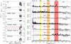 |
Fig. B.1 Time series (left column) and GLS periodograms (right column) of the RV measurements and CCF profile variation diagnostics, as extracted from the HARPS spectra of TOI-282. On the left, the red curves in the second, fourth, and fifth panels represent the linear and quadratic trends, and the sine function, as derived from the best fit to the highest peak detected in the corresponding GLS periodogram. On the right, the horizontal dotted red lines mark the 0.1% false alarm probability (FAP). The shaded areas in yellow, orange, and red mark the rotation frequency frot, and its first and second harmonics (2frot and 3frot), along with their 1σ confidence intervals. The transit frequencies fb, fc, and fd of the three planets are marked with vertical blue dotted lines. |
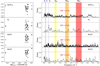 |
Fig. B.2 Time series (left column) and GLS periodograms (right column) of the HARPS activity indicators, namely |
![Mathematical equation: $\[\mathrm{R}_{\mathrm{HK}}^{\prime}\]$](/articles/aa/full_html/2025/12/aa56791-25/aa56791-25-eq74.png)
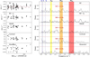 |
Fig. B.3 Time series (left column) and GLS periodograms (right column) of the RV measurements and CCF profile variation diagnostics, as extracted from the ESPRESSO 2nd data set of TOI-282. On the left, the red curve in the first panel represents the best-fitting sine function, as derived by fixing period Pb and mid-time of reference transit T0,b of TOI-282b, while fitting for RV amplitude and offset. On the right, the horizontal dotted red lines mark the 0.1% false alarm probability (FAP). The shaded areas in yellow, orange, and red mark the rotation frequency frot, and its first and second harmonics (2frot and 3frot), along with their 1σ intervals. The transit frequencies fb, fc, and fd of the three planets are marked with vertical blue dotted lines. |
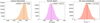 |
Fig. B.4 Posterior distributions of the relevant model parameters outputted by the MCMCI for TOI-282 b: impact parameter (left panel), transit depth (middle panel), and RV semi-amplitude (right panel). |
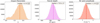 |
Fig. B.5 Posterior distributions of the relevant parameters outputted by the MCMCI for TOI-282 c: impact parameter (left panel), transit depth (middle panel), and RV semi-amplitude (right panel). |
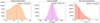 |
Fig. B.6 Posterior distributions of the relevant parameters outputted by the MCMCI for TOI-282 d: impact parameter (left panel), transit depth (middle panel), and RV semi-amplitude (right panel). |
Transit times of TOI-282 b from the LCs + RVs MCMCI analysis with TTVs
Transit times of TOI-282 c from the LCs + RVs MCMCI analysis with TTVs
Transit times of TOI-282 d from the LCs + RVs MCMCI analysis with TTVs
Posteriors and derived orbital parameters (MAP and HDI) for TOI-282 b, c, and d obtained from the dynamical analysis with TRADES
Polynomial detrending baseline models.
All Tables
Main identifiers, equatorial coordinates, parallax, distance, optical and near-infrared magnitudes, and fundamental parameters of the star TOI-282.
Radial velocity measurements, full width at half maximum (FWHM), contrast, and skewness extracted from the cross-correlation functions of TOI-282’s HARPS spectra.
Ca II H&K lines chromospheric index (log ) and Na D1, Na D2, and Hα lines activity indicators extracted from the TOI-282’s HARPS spectra.
Radial velocity measurements, full width at half maximum (FWHM), contrast, and skewness extracted from the cross-correlation functions of the TOI-282’s ESPRESSO spectra.
Posteriors and derived orbital parameters (MAP and HDI) for TOI-282 b, c, and d obtained from the dynamical analysis with TRADES
All Figures
|
Fig. 1 From top to bottom: folded TESS transit light curves of TOI-282 b, c, and d. The photometric data points are plotted with light-blue circles. The dark blue circles mark the 30-minute binned data points. The best-fitting models are over-plotted with red curves. The lower panels display the residuals of the models. |
| In the text | |
|
Fig. 2 From top to bottom: folded RV stellar signals induced by TOI-282 b, c, and d, and best-fitting RV models (red curve). The data includes 37 HARPS spectra (blue circular points) and 8 + 36 ESPRESSO spectra (cyan triangular and green square points, respectively). The lower panels show the residuals to the models. |
| In the text | |
|
Fig. 3 Observed minus calculated (O–C) TTV diagram for TOI-282b, showing TTV as a function of time. The shaded regions represent the 1,2, and 3σ confidence interval derived from the posterior distributions of the model parameters of our dynamical analysis. |
| In the text | |
|
Fig. 4 Observed minus calculated (O–C) TTV diagrams for TOI-282 c (upper panel) and TOI-282d (lower panel), showing TTV as a function of time. The shaded regions represent the 1,2, and 3σ confidence interval derived from the posterior distributions of the model parameters of our dynamical analysis. Both planets exhibit anti-correlated TTV exceeding the transit time uncertainties. |
| In the text | |
|
Fig. 5 Simulated evolution of the orbital parameters over 105 years. Figure b shows a zoom over the first 104 years on the eccentricity and argument of peri-centre plots. The colours blue, red, cyan refer respectively to planets TOI-282b, TOI-282c, TOI-282d. |
| In the text | |
|
Fig. 6 Resonant angle evolution for TOI-282 c and d, for the MAP solutions. The two upper panels show the evolution of the critical angles for the 3:2 resonance (ϕc and ϕd); the lower panel shows the difference between the longitudes of pericentre (Δϖ). |
| In the text | |
|
Fig. 7 Mass-radius diagram showing the position of TOI-282b (Teq = 867 ± 16 K), TOI-282 c (Teq = 643 ± 12 K), and TOI-282 d (Teq = 561 ± 11 K) with respect to the transiting planets whose masses and radii are known with a precision better than 30% and 10%, respectively (circles). The coloured lines show the theoretical models from Zeng et al. (2019). |
| In the text | |
|
Fig. B.1 Time series (left column) and GLS periodograms (right column) of the RV measurements and CCF profile variation diagnostics, as extracted from the HARPS spectra of TOI-282. On the left, the red curves in the second, fourth, and fifth panels represent the linear and quadratic trends, and the sine function, as derived from the best fit to the highest peak detected in the corresponding GLS periodogram. On the right, the horizontal dotted red lines mark the 0.1% false alarm probability (FAP). The shaded areas in yellow, orange, and red mark the rotation frequency frot, and its first and second harmonics (2frot and 3frot), along with their 1σ confidence intervals. The transit frequencies fb, fc, and fd of the three planets are marked with vertical blue dotted lines. |
| In the text | |
|
Fig. B.2 Time series (left column) and GLS periodograms (right column) of the HARPS activity indicators, namely |
| In the text | |
|
Fig. B.3 Time series (left column) and GLS periodograms (right column) of the RV measurements and CCF profile variation diagnostics, as extracted from the ESPRESSO 2nd data set of TOI-282. On the left, the red curve in the first panel represents the best-fitting sine function, as derived by fixing period Pb and mid-time of reference transit T0,b of TOI-282b, while fitting for RV amplitude and offset. On the right, the horizontal dotted red lines mark the 0.1% false alarm probability (FAP). The shaded areas in yellow, orange, and red mark the rotation frequency frot, and its first and second harmonics (2frot and 3frot), along with their 1σ intervals. The transit frequencies fb, fc, and fd of the three planets are marked with vertical blue dotted lines. |
| In the text | |
|
Fig. B.4 Posterior distributions of the relevant model parameters outputted by the MCMCI for TOI-282 b: impact parameter (left panel), transit depth (middle panel), and RV semi-amplitude (right panel). |
| In the text | |
|
Fig. B.5 Posterior distributions of the relevant parameters outputted by the MCMCI for TOI-282 c: impact parameter (left panel), transit depth (middle panel), and RV semi-amplitude (right panel). |
| In the text | |
|
Fig. B.6 Posterior distributions of the relevant parameters outputted by the MCMCI for TOI-282 d: impact parameter (left panel), transit depth (middle panel), and RV semi-amplitude (right panel). |
| In the text | |
Current usage metrics show cumulative count of Article Views (full-text article views including HTML views, PDF and ePub downloads, according to the available data) and Abstracts Views on Vision4Press platform.
Data correspond to usage on the plateform after 2015. The current usage metrics is available 48-96 hours after online publication and is updated daily on week days.
Initial download of the metrics may take a while.