| Issue |
A&A
Volume 704, December 2025
|
|
|---|---|---|
| Article Number | A238 | |
| Number of page(s) | 16 | |
| Section | Galactic structure, stellar clusters and populations | |
| DOI | https://doi.org/10.1051/0004-6361/202556891 | |
| Published online | 18 December 2025 | |
Unveiling the nature of HE 0107–5240: a long period binary CEMP-no star with [Fe/H] of –5.56★
1
LIRA, Observatoire de Paris, Université PSL, Sorbonne Université, Université Paris Cité, CY Cergy Paris Université, CNRS,
92190
Meudon,
France
2
INAF-OATS,
Via G.B.Tiepolo 11,
Trieste
34143,
Italy
3
Leibniz-Institut für Astrophysik (AIP),
An der Sternwarte 16,
14482
Potsdam,
Germany
4
Institute for Fundamental Physics of the Universe (IFPU),
Via Beirut 2,
I34151
Grignano, Trieste,
Italy
5
Zentrum für Astronomie der Universität Heidelberg, Landesstern-warte,
Königstuhl 12,
69117
Heidelberg,
Germany
6
Instituto de Astrofísica de Canarias,
Vía Láctea,
38205
La Laguna, Tenerife,
Spain
7
Universidad de La Laguna, Departamento de Astrofísica,
38206
La Laguna, Tenerife,
Spain
8
Centro de Astrobiología (CSIC-INTA),
Carretera Ajalvir km 4,
28850
Torrejón de Ardoz, Madrid,
Spain
9
Universidad Andres Bello, Facultad de Ciencias Exactas, Departa-mento de Física y Astronomía – Instituto de Astrofísica, Autopista Concepción-Talcahuano
7100,
Talcahuano,
Chile
10
Istituto Nazionale di Astrofisica – Osservatorio Astronomico di Roma (INAF – OAR),
Via Frascati 33,
00040
Monteporzio Catone,
Italy
11
Istituto Nazionale di Fisica Nucleare – Sezione di Perugia (INFN),
via A. Pascoli s/n,
06125
Perugia,
Italy
12
Kavli Institute for the Physics and Mathematics of the Universe, Todai Institutes for Advanced Study, University of Tokyo,
Kashiwa,
277-8583
(Kavli IPMU, WPI),
Japan
13
Istituto Nazionale di Astrofisica – Istituto di Astrofisica e Planetolo-gia Spaziali (INAF – IAPS),
Via Fosso del Cavaliere 100,
00133,
Roma,
Italy
14
Monash Centre for Astrophysics (MoCA), School of Mathematical Sciences, Monash University,
Victoria
3800,
Australia
15
Dipartimento di Fisica, Sapienza Università di Roma,
P.le A. Moro 5,
Roma
00185,
Italy
16
Istituto Nazionale di Fisica Nucleare – Laboratori Nazionali del Sud (INFN – LNS),
Via Santa Sofia 62,
Catania,
Italy
17
Konkoly Observatory, Research Centre for Astronomy and Earth Sciences, Eötvös Loránd Research Network (ELKH),
Konkoly Thege Miklós út 15–17,
1121
Budapest,
Hungary
18
CSFK, MTA Centre of Excellence,
Konkoly Thege Miklós út 15–17,
1121
Budapest,
Hungary
19
Goethe University Frankfurt, Institute for Applied Physics (IAP),
Max-von-Laue-Str. 12,
60438
Frankfurt am Main,
Germany
20
UPJV, Université de Picardie Jules Verne,
33 rue St Leu,
80080
Amiens,
France
21
European Southern Observatory,
Casilla
19001,
Santiago,
Chile
22
Instituto de Astrofísica e Ciências do Espaço, Universidade do Porto, CAUP,
Rua das Estrelas,
4150-762
Porto,
Portugal
23
Centro de Astrofísica da Universidade do Porto,
Rua das Estrelas,
4150-762
Porto,
Portugal
24
Centre for Astrophysics and Supercomputing, Swinburne University of Technology,
Hawthorn,
Victoria
3122,
Australia
25
Instituto de Astrofísica e Ciências do Espaço, Faculdade de Ciên-cias da Universidade de Lisboa,
Campo Grande,
1749-016
Lisboa,
Portugal
26
Departamento de Física e Astronomia, Faculdade de Ciências, Universidade do Porto,
Rua do Campo Alegre,
4169-007
Porto,
Portugal
27
Observatoire Astronomique de l’Université de Genève,
Chemin Pegasi 51,
Sauverny
1290,
Switzerland
★★ Corresponding author.
Received:
18
August
2025
Accepted:
9
October
2025
Abstract
Context. The vast majority of the most iron-poor stars in the Galaxy exhibit strong carbon enhancement, with C/H ratios about two orders of magnitude below solar. This unusual chemical composition likely reflects the properties of the gas cloud from which these stars formed, having been enriched by one, or at most a few, supernovae. A remarkable member of this stellar class, HE 0107 −5240 with [Fe/H]=–5.56, has been identified as part of a binary system.
Aims. We aim to constrain the orbital parameters of HE 0107−5240 through radial velocity monitoring with the ESPRESSO spectrograph.
Methods. We derived radial velocities using cross-correlation with a template, taking advantage of the strong G-band feature. We combined all observations to obtain a high signal-to-noise ratio spectrum, which we used to refine our understanding of the stellar chemical composition. We additionally used a co-added UVES spectrum in the blue to complement the wavelength coverage of ESPRESSO.
Results. Observations of HE 0107−5240 over a span of more than four years yield a revised orbital period of about 29 years. We provide updated elemental abundances for Sc, Cr, Co, and, tentatively, Al, along with a new upper limit for Be. We derive the iron abundance from ionised Fe lines and establish significant upper limits for Li, Si, and Sr.
Conclusions. We confirm that the star is a long-period binary. Iron abundances derived from neutral and ionised lines are consistent with the local thermodynamical equilibrium (LTE) assumption, which casts doubt on published deviations from LTE corrections for Fe in this star. The heavy elements Sr and Ba remain undetected, confirming the classification of HE 0107−5240 as a carbon-enhanced, metal-poor star not enhanced in heavy elements (CEMP-no), and supporting the absence of an n-capture element plateau at the lowest metallicities.
Key words: stars: abundances / stars: Population II / stars: Population III / Galaxy: abundances / Galaxy: evolution / Galaxy: formation
Based on ESPRESSO GTO observations collected under ESO programmes 0103.D-0700 and 108.2268.001 (PI: P. Molaro), 1104.C-0350 1102.C-0744 (PI: F. Pepe), and 114.27NH.001 (PI: D. Aguado).
© The Authors 2025
 Open Access article, published by EDP Sciences, under the terms of the Creative Commons Attribution License (https://creativecommons.org/licenses/by/4.0), which permits unrestricted use, distribution, and reproduction in any medium, provided the original work is properly cited.
This article is published in open access under the Subscribe to Open model. This email address is being protected from spambots. You need JavaScript enabled to view it. to support open access publication.
1 Introduction
The metal-poor stars we observe today likely formed shortly after the Big Bang, from gas clouds that were only slightly enriched by one or a few supernovae. Given their lifetimes, which are comparable to the age of the Universe, these stars must have low masses (M < 0.8 M⊙). Metal-poor stars have been known since the early work of Chamberlain & Aller (1951), but it was the HK survey by Beers et al. (1992) that led to the discovery of a distinct group: carbon-enhanced, iron-poor stars. Within this group, researchers identified a subclass that combines high carbon enhancement with a deficiency or absence of n-capture elements (Norris et al. 1997; Bonifacio et al. 1998). The star HE 0107−5240 was discovered at the beginning of this century (Christlieb et al. 2002) and has since become the prototype of this rare class, which now includes the majority of the most iron-poor stars identified.
Currently, about a dozen stars are known with extremely low iron abundances ([Fe/H] < −4.5) and relatively high carbon abundances (5.5 < A(C) < 7.8). Only two known stars in this regime (SDSS J102915.14+172927.9 Caffau et al. 2011a and Pristine J221.8781+09.7844 Starkenburg et al. 2018) do not exhibit carbon enhancement, showing only upper limits on their carbon abundances: A(C) < 4.68 for the former (Caffau et al. 2024b) and below 6.0 for the latter (Lardo et al. 2021). Recently, Limberg et al. (2025) report an evolved star that does not show C in its spectrum. After accounting for C converted into N, the upper limit is just A(C) < 4.79 ([C/Fe] < +1.18).
Unevolved warm stars (Teff > 5800 K) often display a weak G-band, making carbon abundance determinations challenging and complicating the identification of extremely metal-poor (EMP) stars that are not carbon-enhanced metal-poor (CEMP), here defined as [C/Fe] > 1.0 Beers & Christlieb 2005). According to Bonifacio et al. (2015), CEMP-no stars show a relatively constant absolute carbon abundance, lower than that of CEMP-s stars, which also show enhanced abundances of s-process elements. The carbon in CEMP-s stars likely originates from mass transfer from an evolved asymptotic giant branch (AGB) companion, along with elements such as Sr and Ba. In contrast, the carbon in CEMP-no stars is likely primordial. The so-called ‘low-carbon band’ (Bonifacio et al. 2015) is centred around A(C) ∼ 6.8. We therefore suggest that in the ultra iron-poor regime ([Fe/H] < −4.5), stars with A(C) > 5.8 should be classified as CEMP, rather than relying solely on [C/Fe] > 1.
It is plausible that carbon-normal and carbon-enhanced ultra-iron-poor stars have distinct origins. For example, SDSS J102915.14+172927.9 exhibits a solar-scaled abundance pattern without the typical α-element enhancement seen in most metal-poor stars and it follows an orbit in the Galactic disc. This may indicate that this is a Pop III star and that its stellar surface was polluted during its long journey through the Galactic disc (see Caffau et al. 2024b).
The star HE 0107−5240 was first reported by Christlieb et al. (2002), with a detailed chemical abundance analysis presented by Christlieb et al. (2004) based on Ultra Violet Echelle Spectrograph (UVES) spectra. The oxygen abundance was later derived from OH molecular lines in the UV by Bessell et al. (2004). The impact of 3D hydrodynamic models on the inferred abundances was explored by Collet et al. (2006), while deviations from local thermodynamic equilibrium (LTE) were examined using non-local thermodynamic equilibrium (NLTE) calculations for iron by Ezzeddine et al. (2017) and for Mg and Ca by Sitnova et al. (2019).
The star HE 0107−5240 was included in an ESO ESPRESSO1 GTO programme, which investigates binarity among the most metal-poor stars. Its binary nature was first suggested by Arentsen et al. (2019), who note discrepancies between the radial velocities measured with UVES and SALT HRS2. This was subsequently confirmed by Bonifacio et al. (2020) using early ESPRESSO data. Aguado et al. (2022) analysed continued ESPRESSO monitoring over more than three years and derived a long orbital period of approximately 13 000 days (∼36 years), showing that binary formation is not precluded at extremely low metallicities. Aguado et al. (2022) also measured a carbon isotopic ratio of 12C/13C = 87±6. This value excludes mass transfer from an evolved AGB companion as the source of the observed carbon and implies a significant primordial production of 13C in the progenitor. In the present study, we extend the temporal baseline of radial velocity monitoring and analyse a new, high signal-to-noise, co-added spectrum derived from all the available ESPRESSO observations.
2 Observations
HE 0107−5240 was observed as part of several ESPRESSO GTO programmes: 0103.D-0700, 108.2268.001, and 110.245W.001 (PI: P. Molaro); 1102.C-0744 and 1104.C-0350 (PI: F. Pepe); and during the open-time programme 114.27NH.001 (PI: D. S. Aguado). We reduced all observations in the same way. We complemented the GTO data, previously analysed by Aguado et al. (2022) and Molaro et al. (2023), with the additional open-time observations. All spectra cover the same wavelength range from 380 to 788 nm; we corrected them for the star’s orbital motion, co-added them, and used them for a revised chemical abundance analysis.
Because the ESPRESSO spectrum extends only to approximately 380 nm in the blue, we used UVES data to study chemical species with transitions in the ultraviolet. The UVES spectra consist of a sequence of observations using the 346 nm setting, obtained between September 30 and December 27, 2002, for a total exposure time of 19.5 hours (see Bonifacio et al. 2021, for the observation log). A total of 22 observing blocks (OBs) were available from programme 70.D-0009, of which 21 were usable (one OB was exposed for only 1 s and contained no signal). Most OBs had exposure times of 3600 s, with three exceptions at 1727, 1600, and 3960 s, respectively. The combined UVES spectrum reached a signal-to-noise ratio (S/N) of approximately 50 per pixel at 324 nm.
We shifted the individual UVES spectra to the rest frame, scaled them relative to one another, and co-added them using an iterative κσ-clipping procedure to compute a weighted average while removing outliers. Because the pixel scale was 0.215′′ per pixel in the blue arm of UVES, the resulting spectrum was oversampled. We therefore rebinned it by a factor of two. The final co-added spectrum achieves a peak S/N per 0.05 Å pixel of ∼140 at 3800 Å, decreasing to S/N ∼70 at 3350 Å and ∼30 at 3100 Å. Arentsen et al. (2019) derived radial velocities from SALT HRS spectra and we used their radial velocities.
3 Galactic kinematics
We adopted coordinates, proper motions, and parallax from Gaia DR3 (Gaia Collaboration 2023), applying the parallax zero-point correction as prescribed by Lindegren et al. (2021). The distance derived from the parallax is  . The star is part of a binary system, although the faint companion is not directly visible. Radial velocity variations have been extensively discussed by Aguado et al. (2022) and Molaro et al. (2023). For our analysis, we adopted the systemic (barycentric) radial velocity of the system, Vrad = 46.6 ± 0.1 kms−1 (see Sect. 4), and used this value to derive the star’s Galactic orbit.
Following the procedure described in Caffau et al. (2024a), we employed the galpy code (Bovy 2015) with the MWPo-tential2014 Galactic potential model. We integrated the orbit backwards in time over 1 Gyr. For solar motion, we adopted the parameters from Schönrich et al. (2010), assuming a solar distance to the Galactic centre of 8 kpc and a circular velocity of 220 kms−1 (Bovy et al. 2012).
The kinematical properties of the star are shown in Fig. 1. The upper and lower panels display its position in several diagnostic diagrams: the Toomre diagram (top-left), orbital energy versus angular momentum (top-right), the square root of the radial action versus the azimuthal action (bottom-left), and the action diamond (bottom-right). The star is marked with a black star symbol. For comparison, stars from the good-parallax sample of Bonifacio et al. (2021, coloured points) are also plotted. Based on the classification criteria of Bensby et al. (2014), thin disc, thick disc, and halo stars are shown in red, green, and blue, respectively. The red and green shaded boxes in the bottom panels correspond to the regions defined by Feuillet et al. (2021) for stars associated with the Gaia-Sausage-Enceladus (GSE; red box, bottom-left) and Sequoia (green box, bottom-right) accretion events.
Sestito et al. (2019) estimate a distance of 14.3 ± 1.0 kpc and classify the system as having a retrograde Galactic halo orbit with an apocentric radius of rap = 15.9 kpc. We adopted a significantly shorter distance of 6.93 kpc. According to the Bensby et al. (2014) criteria, the system is classified as a thick disc star, consistent with its location in the kinematic diagrams of Fig. 1. However, its vertical distance from the Galactic plane (z = −6.2 kpc), maximum orbital height (Zmax ≈ 6.3 kpc), and apocentric distance (rap = 9.9 kpc) suggest otherwise. The orbit is eccentric (e = 0.69) and prograde, with positive angular momentum (LZ) and transverse velocity (vT). Moreover, the star does not appear to be associated with either the GSE or Sequoia structures. We therefore conclude that HE 0107−5240 is best classified as a halo star on a prograde Galactic orbit.
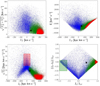 |
Fig. 1 Top panels: position of HE 0107−5240 (filled black star) in the Toomre diagram (left) and the orbital energy versus angular momentum (right). Bottom panels: square root of the radial action versus the azimuthal action (left) and action diamond (right). Coloured points represent stars from the good-parallax sample of Bonifacio et al. (2021). The red and green shaded areas indicate the regions defined by Feuillet et al. (2021) to select candidate Gaia-Sausage-Enceladus (GSE) and Sequoia stars. |
4 Orbital parameters
We recomputed the orbital parameters of the binary star HE 0107−5240 considering the new measurements of radial velocities, including those from the first three years of observations, to benefit from a better template in the cross-correlation analysis. The new measurements from the ESPRESSO spectra are provided in Table 1. For the UVES and HRS at SALT spectra, we used the measurements provided in Bonifacio et al. (2020) and Arentsen et al. (2019). For the HARPS spectrum, we used the measurements provided in Aguado et al. (2022). With respect to the epochs provided in Aguado et al. (2022)3, we rejected a few measurements obtained from very low S/N spectra. The whole set of ESPRESSO radial velocities (RVs) follows a decreasing trend, as expected for this long-period binary. The vrad data are binned in intervals of one day to minimise the stellar jitter (see Fig. 2, upper-left panel). The RVs are modelled using the RAD-VEL code (Fulton et al. 2018)4 including the Keplerian motion of the star, an RV offset (the γ of the vrad curve), and a jitter parameter for each instrument, within a likelihood scheme implemented in Python using CELERITE (Foreman-Mackey et al. 2017)5.
The Keplerian orbit for the radial velocity is described as
 (1)
where the true anomaly, νa, is a function of the eccentric anomaly, E, which is, in turn, a function of time, through Kepler’s equation (see Equations (1)–(3) in Fulton et al. 2018). The five parameters that define the orbit are the orbital period (P2), the orbital semi-amplitude velocity (k2), the angle of periastron (ω), the eccentricity (e), and the time of passage at periastron (T2,peri). The RADVEL program provides estimates of both the time of periastron, T2,peri, and the time of the inferior conjunction of the star, T2,conj. An orbit can be fitted using any set of independent parameters derived from these five. Following Fulton et al. (2018), we performed fitting and posterior sampling using the ln P2, T2,conj,
(1)
where the true anomaly, νa, is a function of the eccentric anomaly, E, which is, in turn, a function of time, through Kepler’s equation (see Equations (1)–(3) in Fulton et al. 2018). The five parameters that define the orbit are the orbital period (P2), the orbital semi-amplitude velocity (k2), the angle of periastron (ω), the eccentricity (e), and the time of passage at periastron (T2,peri). The RADVEL program provides estimates of both the time of periastron, T2,peri, and the time of the inferior conjunction of the star, T2,conj. An orbit can be fitted using any set of independent parameters derived from these five. Following Fulton et al. (2018), we performed fitting and posterior sampling using the ln P2, T2,conj,  ,
,  , and ln k2 basis, which helps to speed up convergence. We chose ln k2 to avoid favouring large k2, and ln P2 because P2 may be long when compared with the observational baseline. The vrad errors in Fig. 2 include the jitter of each instrument, and the vrad offset has been subtracted. In addition, we adopted uniform priors for all parameters (see Table 2). The revised orbital period of the system is 28.9 ± 2 yr. However, since the time during which we have been observing this system is shorter than the best-fit period, the actual uncertainty on the period could be larger than our estimate.
To sample the posterior distributions and obtain the Bayesian evidence of the model (that is, the marginal likelihood, ln Z), we used nested sampling via DYNESTY (Speagle 2020)6. We initialised a number of live points equal to N3(N + 1) to efficiently sample the parameter space, with N = 10 being the number of free parameters. In the middle panel of Fig. 2, we show in grey a subsample of 300 models randomly selected from the final ∼37 696 Bayesian samples of the posterior distributions. The binary mass function can be computed from the masses of the binary component (e.g. Tauris & van den Heuvel 2006), i.e. that of the observed star, M2, and that of the unseen binary companion, M1, together with the orbital parameters as follows:
 (2)
(2)
![Mathematical equation: $f({\rm{M}}) = \left[ {\left( {{P_{{\rm{orb}}}}k_2^3} \right)/(2\pi G)} \right]{\left( {1 - {e^2}} \right)^{3/2}}.$](/articles/aa/full_html/2025/12/aa56891-25/aa56891-25-eq6.png) (3)
(3)
From the Bayesian samples, we computed the posterior distribution of the binary mass function providing the following result:
![Mathematical equation: $f({\rm{M}}) = 47_{ - 6}^{ + 8} \times {10^{ - 4}}\left[ {{M_ \odot }} \right].$](/articles/aa/full_html/2025/12/aa56891-25/aa56891-25-eq17.png) (4)
(4)
The binary mass function provides a lower limit to the mass of the unseen companion. The minimum mass of the companion can be estimated as the maximum value between f and  . Adopting a mass of M2[M⊙] = 0.8 for the visible star, we obtain M1[M⊙] > 0.14 for the unseen companion. The minimum orbital distance (that is, the semi-major axis) of the star with respect to the centre of mass of the binary system can be computed as
![Mathematical equation: ${a_2}\sin i = \left[ {\left( {{P_{{\rm{orb}}}}{k_2}} \right)/(2\pi )} \right]{\left( {1 - {e^2}} \right)^{1/2}} = 1.571_{ - 0.100}^{ + 0.153}{\rm{AU}}.$](/articles/aa/full_html/2025/12/aa56891-25/aa56891-25-eq19.png) (5)
(5)
The dispersion of the ESPRESSO radial velocities, after subtracting the best fit, is now 47 m s−1, which is consistent with the derived velocity jitter (Table 2). However, this value is about three times higher than the mean error bar of the ESPRESSO radial velocity measurements, suggesting the presence of additional signal of relatively smaller amplitude. Pulsations, stellar activity, or the presence of planetary motion are discussed in Aguado et al. (2022). The residuals of the ESPRESSO RVs, shown in the inset within the centre panel of Fig. 2 after subtracting the orbital solution (black line), were analysed for periodicity and did not show any obvious peak in the periodogram.
Log of the ESPRESSO observations and radial velocity measurements.
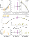 |
Fig. 2 Radial velocities (RV) of HE 0107−5240 versus heliocentric Julian date (HJD), together with the best-fit RV model. The inset within the middle panel shows ESPRESSO RV points after subtracting the best-fit model. The root mean square (RMS) of all residuals is indicated in the middle panel, while the RMS values from each spectrograph are given in the bottom panels. |
Revised orbital parameters of HE 0107−5240 derived using a Markov chain Monte Carlo (MCMC) analysis.
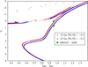 |
Fig. 3 Isochrones from the BASTI database (Pietrinferni et al. 2021) in a Gaia colour-magnitude diagram. The two green points correspond to HE 0107−5240, assuming surface gravities of log g = 2.20 (upper point) and 2.46 (lower point), respectively. |
5 Chemical analysis
5.1 Stellar parameters
Using Gaia DR3 (Gaia Collaboration 2023) photometry and parallax corrected by the zero-point (−0.03783 mas) as suggested by Lindegren et al. (2021), with reddening Av = 0.0344 from Schlafly & Finkbeiner (2011), we derive: Teff= 5111 K and log g = 2.46 [cgs], as described in Caffau et al. (2024b). If the zero-point correction is not applied, the derived stellar parameters are Teff = 5116 K and log g= 2.20 [cgs]. Using the surface gravity derived with zero-point correction applied, the position of the star in a Gaia colour-magnitude diagram (CMD) agrees well with a BASTI isochrone (Bag of Stellar Tracks and Isochrones, Pietrinferni et al. 2021) for an age of 13 Gyr and [Fe/H] = −2.2 (see Fig. 3). The mass range implied by the two surface gravities is 0.77–0.78 M⊙. If the zero point is not applied, the position of the star remains compatible with the [Fe/H] = −2.2 isochrone, but agrees better with that of the same age and [Fe/H] = −3.2. The position of HE 0107−5240, when using parameters corrected by the zero point, in the Gaia CMD matches only marginally with a BASTI isochrone for an age of 13 Gyr and [Fe/H] = −3.2 (this is the lowest [Fe/H] value provided by BASTI isochrones). The metallicity of HE 0107−5240 is log Z/Z⊙ ≈ −2.4, due to its very high overabundance of CNO with respect to Fe. The high carbon abundance leads to strong CH lines in the blue and UV spectral ranges, causing the star to appear significantly redder in the GBP − GRP colour than stars with a scaled solar abundance pattern. This could explain why a star with [Fe/H] = −5.56 (Aguado et al. 2022) is compatible with an isochrone 2–3 dex more metal-rich. However, it should be noted that to build the isochrones, regardless of the position in the HR diagram, all the models were computed with the same mixing-length value. This is especially problematic for evolved stars (see Manchon et al. 2024), as clearly discussed in the sample of giant stars investigated by Caffau et al. (2025).
Regarding reddening, we note that the star has a very low extinction. This is confirmed by the absence of diffuse interstellar bands (DIBs) in the high-quality ESPRESSO spectrum. The interstellar Na I doublet lines are visible but weak, and their equivalent widths confirm the low extinction. In fact, the position of HE 0107−5240 in the sky (l = 296.5° and b = −64.49°) coincides with a well-known window in the local interstellar matter, where the photons from the star intercept relatively small clouds in the solar vicinity.
The stellar parameters used in the analyses of this star in the literature (see Table A.1) are: Teff = 5100 K and log g = 2.2 (Christlieb et al. 2002, 2004; Bessell et al. 2004; Yong et al. 2013; Aguado et al. 2022; Molaro et al. 2023); Teff = 5130 K and log g = 2.2 (Collet et al. 2006); Teff = 5050 K and log g = 2.3 (Ezzeddine et al. 2017); and Teff = 5300 K and log g = 2.5 (Sitnova et al. 2019). We adopted Teff = 5100 K, log g = 2.2, and a microturbulence of 2.2 kms−1, to remain consistent with previous works, particularly Christlieb et al. (2004), Aguado et al. (2022), and Molaro et al. (2023). The latter two studies analysed a combined spectrum derived from the same ESPRESSO observations but based on fewer exposures.
Using the Gaia parallax, the G magnitude, and the bolo-metric correction derived from the grid of ATLAS 9 fluxes7, we estimated the luminosity of the star as log(L/L⊙) = 1.67 ± 0.02. The uncertainty accounts for the errors in both the parallax and G-magnitude, but is dominated by the parallax error. Although red giant stars are not in a very favourable position in the Hertzsprung-Russel diagram for age determination, we attempted to estimate the age using the SPInS code (Stellar Parameters Inferred Systematicall Lebreton & Reese 2020; Reese & Lebreton 2020). We used a grid of BASTI α-enhanced evolutionary tracks (Pietrinferni et al. 2006). The input parameters were log(Teff), log(L/L⊙), and log(Z). This choice ensures that the parameters of HE 0107−5240 lie well within the range covered by the grid. Had we chosen [Fe/H] as metallicity indicator, the value for HE 0107−5240 would fall outside the grid. In the inference, we assumed a uniform prior on age, requiring it to be smaller than the age of the Universe, 13.8 Gyr (Planck Collaboration 2020). The resulting age is 7.6 Gyr±3.2 Gyr.
5.2 Spectral energy distribution
The VOSA (Virtual Observatory Sed Analyzer) service8 provides the best-fitting parameters of Teff = 5500 K and log g = 1.5. They indicate a considerably higher Teff than our adopted one, and lower surface gravity (see Sect. 5.1). The spectral energy distribution of the star, when compared with the flux derived from the model, does not show any UV or IR excess.
5.3 Abundances
HE 0107−5240 is ultra-poor in Fe, but its C content is about 16% of the solar value, which makes it a CEMP star. Table A.1 lists the abundances derived in the literature. As expected, several upper-limits are reported; however, owing to the star’s very low metallicity, many of them are too high to be significant. In particular, the upper limits for the heavy elements do not allow us to determine whether HE 0107−5240 meets the criterion for a CEMP-no star. Abundances or upper-limits derived from the new high-quality spectrum are provided in Table A.2 and an element-by-element discussion is given below. For the main 1D LTE analysis, we performed spectral synthesis using SYNTHE with an ATLAS 9 model atmosphere (Kurucz 2005). In addition, we computed dedicated 3D model atmospheres with the CO5BOLD code (COnservative COde for the COmputation of COmpressible COnvection in a BOx of L Dimensions Freytag et al. 2012, plus updates) to estimate 3D (LTE) corrections for selected spectral lines. Details about the models and spectrum synthesis codes are provided in the Appendix (B).
Lithium. Lithium absorption from the Li I doublet at 670.7 nm is not detected. We applied Cayrel’s formula9, multiplied by a factor of three to account for the uncertainty at 3σ (see Cayrel 1988, S/N=230), and obtained A(Li) < −0.14 dex.
Beryllium. The two Be II resonance doublet lines lie at 313.0442 and 313.1067 nm, both outside the wavelength coverage of ESPRESSO. The reddest Be II feature (313.1067 nm) is not clearly detected in the UVES spectrum (see Fig. 4), while the other line (313.0442 nm) is heavily blended with CH molecular features. If present, the 313.1 nm line is buried in the noise, with S/N ∼ 35. We therefore derive an upper limit (or tentative detection) of A(Be) ⪅ −2.06, corresponding to [Be/H] ⪅ −3.44 and [Be/Fe] ⪅ +2.12. However, we note that a weak feature is visible at the expected position of the line. If confirmed, this feature could originate from primary spallation processes involving energetic CNO particles from the progenitor of HE 0107−5240 colliding with the ambient medium. Even an upper limit slightly above [Be/Fe] < +2.0 dex is significant (assuming the star has not depleted its beryllium), as it argues against the existence of a primordial Be plateau (see Figure 5) predicted by certain inhomogeneous cosmological models, albeit at lower abundance levels (Malaney & Fowler 1989; Thomas et al. 1994; Jedamzik & Rehm 2001; Nakamura & Hashimoto 2017).
Carbon. The new spectrum does not alter the derived carbon abundance, as the CH G-band features are so strong that they do not benefit from an increased S/N. To determine the carbon isotopic ratio, we selected regions in the observed spectrum where clean pairs of 12CH and 13CH lines are present. These lines arise from the same electronic transitions, but the 12CH features are significantly stronger because the stellar atmosphere contains approximately two orders of magnitude more 12C than 13C.
Our approach differs from that of Molaro et al. (2023) in that we used different spectral regions and simultaneously fitted both the total carbon abundance and the isotopic ratio. We selected five wavelength intervals containing matched 12CH and 13CH lines and performed a global fit treating both parameters as free variables. This analysis yielded (i) a carbon abundance of A(C) = 6.72 ± 0.02, where the uncertainty represents the region-to-region scatter (i.e. a formal error), and (ii) an isotopic ratio of 12C/13C = 110 ± 12. Our carbon abundance is in excellent agreement with the value of A(C) = 6.75 reported by Molaro et al. (2023), and the isotopic ratio is consistent within 1.7σ with their value of 12C/13C = 87 ± 6.
To evaluate the impact of 3D effects, we computed the 3D (LTE) correction for the 12CH line at 423.1 nm, obtaining a correction of −0.65 dex for the 12C abundance. To assess the 3D correction of the isotopic ratio, we focused on the same spectral region, examining pairs of 12CH and 13CH lines that share the same electronic transition. Although both lines experience similar 3D effects at equal line strengths, their strengths differ significantly in practice. For a solar carbon isotopic ratio, the equivalent width (EW) of the 12CH line is tens of times larger than that of the corresponding 13CH line.
We computed the 3D correction factor of the 12C/13C isotopic ratio, Rq, as the ratio of the isotopic ratios derived in 3D and in 1D, Rq = q3D/q1D, and expressed this as a function of q1D for different choices of the 13CH line’s equivalent width, EW13, as shown in Fig. 6. The correction is also sensitive to the adopted microturbulence. We used a value of 1.3 kms−1, selected to ensure a flat 3D abundance correction with the strength of the 516.9 nm Fe II line (see below).
Unfortunately, the derived 3D corrections depend on the chemical composition, in particular the C, N, and O abundances, adopted for the construction of the 3D atmosphere and the 1D reference model. All 3D results reported above are based on a 3D (and 1D reference) model with a solar chemical composition scaled down by −4.0 dex, except for the α elements (including O but not C), which are enhanced by +0.4 dex relative to the other metals. Compared to the abundances derived for HE 0107–5240 in this work, C and O are too low by about −2.3 and −0.65 dex, respectively, in this model.
As an alternative, we also computed a pair of 3D–1D models in which the carbon and nitrogen abundances are enhanced by +3.0 dex and the oxygen abundance by +2.6 dex relative to the previous case. Again, these C, N, and O abundances are not representative of HE 0107–5240; C and O are now too high by about 0.7 and 2.0 dex, respectively. The C/O ratio is ∼0.5 instead of ∼10.
Using the same procedure, we derive the 3D correction for the C abundance and the 3D correction for the 12C/13C isotopic ratio. As already found by Gallagher et al. (2017), the 3D correction is smaller (about −0.2 dex) and the 3D correction factor for the C isotopic ratio increases from approximately 0.8 to 1.1, implying that the 3D-corrected isotopic ratio is larger than that derived in 1D. Importantly, a robust result, beyond all uncertainties of the modelling, is that HE 0107–5240 has a high 12C/13C isotopic ratio (≳ 90), ruling out any mixing with CNO-processed material. More reliable 3D corrections can be obtained only from future 3D models computed using custom-made opacity tables with consistent CNO abundances.
Nitrogen. The NH band at 336 nm lies outside the wavelength coverage of ESPRESSO. We therefore used the UVES 346 spectrum to investigate it. We inspected this 336 nm NH band using the molecular data provided by Fernando et al. (2018) and derive A(N)=4.42 ([N/H] = −3.44 and [N/Fe] = +2.12). The 3D correction for the N abundance from this band is −0.58 dex, which, if applied, would decrease the [N/Fe] ratio to 1.6 dex.
Oxygen. No useful atomic or molecular line is available in the wavelength range of ESPRESSO. The OH lines in the UV range of a UVES spectrum have already been investigated by Bessell et al. (2004). We selected the OH lines listed by Prakapavičius et al. (2017), as the molecular data we adopted are from their Table A.1. We investigated ten OH lines and derive ⟨A(O)⟩ = 5.72 ± 0.09. With a solar oxygen abundance of 8.76 (see Table A.2), we obtained [O/H] = −3.04 and [O/Fe] = +2.52 dex. The 3D effects on molecular lines are strong. The average correction we derive is −0.58 ± 0.07 dex, but it should be emphasised that the corrections were computed without accounting for scattering in the synthesis of both 1D and 3D profiles.
Sodium. The two Na I-D resonance lines are strong in the spectrum, providing an abundance of A(Na)=1.64. According to Andrievsky et al. (2007), NLTE corrections for the Na I D lines are small in the extremely metal-poor regime. Two weak features due to Galactic interstellar absorption account for the very low reddening.
Aluminium. At the wavelength of the strongest Al I line at 396.1 nm, a feature consistent with the Al line is visible. However, on the red side, a noise spike renders the detection uncertain. Either this is a tentative Al detection with an abundance of A(Al) = 0.27, or there is a conservative higher upper limit at A(Al) < 0.47. In both cases, the star is poor in Al, with [Al/Fe] = −0.64 or [Al/Fe] < −0.44 (see Fig. 7). The Al resonance lines are affected by strong NLTE effects. For the well-known star CD–38:245, which has stellar parameters similar to HE 0107−5240, Andrievsky et al. (2008) derived a NLTE correction of +0.74 dex. The NLTE correction for Fe, according to the website10 (hereafter MPIA), is approximately +0.55 dex (see the paragraph on iron below). Taking into account the NLTE corrections for Al and Fe, the star is consistent with a solar [Al/Fe] ratio.
Silicon. The strong Si I line at 390.5 nm is not clearly visible in the spectrum, but there is a hint of a feature that could be attributed to this Si I line. We provide a conservative upper limit of A(Si) < 1.8, corresponding to [Si/Fe] < −0.16. In fact, we identify feature, compatible with noise, at the expected wavelength, corresponding to a lower Si abundance (A(Si) ∼ 1.6, [Si/Fe] ∼ −0.36). For this line, the NLTE corrections provided on the MPIA website are large (+0.31 dex) when adopting a metallicity of −5.0 for the star, but still smaller than the NLTE correction for Fe. At a metallicity of −4.0, the NLTE correction for both elements are much smaller (+0.1 dex for Si and +0.3 dex for Fe).
Sulphur. The strongest S I feature available in the ESPRESSO spectrum is the strongest triplet of Mult. 8 at 675.7 nm. However, this feature is already weak in solar-metallicity or slightly metal-poor stars, and the upper limit we derive (A(S) < 5.2) is not significant. The UVES spectra with the 860 nm setting host the stronger S I lines of Mult. 1. We selected the S I lines at 922.8 and 923.7 nm, which are free from telluric absorption. The averaged spectrum from four OBs provided a more stringent upper limit at A(S) < 4.40 ([S/Fe] < 2.80) but it is still not significant. The S I lines of Mult, 1 are very sensitive to NLTE effects. According to Takeda et al. (2005), the line at 923.7 nm is expected to have an NLTE correction of about −0.5 dex for a metallicity of −4.0.
Potassium. The strong K I line at 769.8 nm is not visible in the spectrum of HE 0107−5240 and no telluric contamination affects the position of the line. We took into account the S/N ratio of 200 and, using Cayrel’s formula, we derive an upper limit of [K/Fe] < 1.50, which is not significant. According to the computations of Andrievsky et al. (2010), the NLTE correction for this line is small, of the order of +0.1 dex.
Scandium. Two Sc II lines (361.38 and 363.07 nm) are available in the UVES 346 spectrum. Despite the low S/N ratio in this spectral region, we detect the 361.3 nm Sc II line and derive A(Sc) = −2.3 ([Sc/H] = −5.40).
Chromium. Due to the good spectral quality (S/N ∼ 100), at 425.43 nm a feature is visible in the spectrum. According to the synthesis, this feature is a mixture of the Cr I line at 425.43 nm with two CH lines, so the contribution is dominated by CH. In the green wavelength range, at 520 nm, the S/N is almost 200, and three Cr I lines are not visible. Using Cayrel’s formula, we derive an upper limit that is too small, and, in our view, too optimistic for such weak lines. We consider an upper limit of A(Cr) < 0.30 and [Cr/Fe] < 0.22 to be reasonable. The Cr upper limit is not significant enough to draw conclusions about the star. Moreover, the NLTE correction is large and positive (+0.8 dex for a metallicity of −4.0) according to MPIA. This value is larger than the NLTE correction for Fe, which renders this upper limit not significant.
Manganese. The Mn I at 403.3 nm is not visible, providing (using Cayrel’s formula) a stringent upper limit of A(Mn) < −0.50. However, the NLTE correction expected from this line is large (∼1 dex; see Bergemann & Gehren 2008).
Iron. We adopt A(Fe)=1.96 from neutral lines as reported by Aguado et al. (2022), as our value derived from the latest combined ESPRESSO spectrum is only 0.005 dex higher. Christlieb et al. (2004) provided upper limits on A(Fe) from two Fe II lines at 501.8440 and 516.9028 nm (Nave & Johansson 2013). Of these lines, the 516.9 nm line is weak but clearly visible in the ESPRESSO spectrum. We adopted log gf = −1.0 from Meléndez & Barbuy (2009), while Schnabel et al. (2004) reported a log g f of −0.87. We derive A(Fe)=1.74 from line-profile fitting (see Fig. 8). From two other Fe II lines expected to be sufficiently strong for detection in extremely metal-poor stars (492.3921 and 501.8440 nm), we derive only upper limits, consistent with the abundance from the 516.9 nm line (see Fig. 8). As expected, according to MPIA, the NLTE correction for the 516.9 nm line is very small (0.03 dex). Our 3D LTE model provides a 3D correction for this line of about +0.1 dex. In the UVES 346 setting, we also detected the Fe II line at 322.774 nm for which we derive A(Fe)=1.67 (with a log g f of −1.014), in good agreement with the Fe II line in the ESPRESSO spectrum.
Among the Fe I lines investigated by Aguado et al. (2022), 12 are present in the MPIA database and were used to derive 1D NLTE corrections for iron. From these lines, we derive an NLTE correction of +0.54, adopting a model with the parameters Teff=5100 K, log g=2.2, [Fe/H] = −5.0, and a microturbulence of 2.2 kms−1 (−5.0 being the lowest metallicity). Applying this NLTE correction to A(Fe)=1.96 derived from Fe I lines results in a disagreement with the abundance from the A(Fe)=1.74 Fe II line. The NLTE correction for the same Fe I line, adopting a metallicity −3.0 (compatible with the oxygen abundance), is +0.12 dex, and for a metallicity of −2.0 (compatible with the carbon content), it is +0.08 dex. Clearly, a ‘high’ NLTE correction in A(Fe) from neutral lines introduces tension with the Fe abundance derived from the ionised lines.
Cobalt. The Co I UV lines at 345.35 and 352.98 nm are outside the ESPRESSO wavelength range, but fall within the UV UVES range. The result from the UVES spectrum is not clear. (i) The feature at 345.35 nm is consistent with A(Co) ∼ −0.30. The line is blended with an NH feature that is not reproduced by the model, but the blend does not affect the derived abundance. (ii) The two Co I lines at 352.9 nm are consistent and provide A(Co) ∼ 0.30 and [Co/H] = −4.62.
Zinc. The line at 481.5 nm is the strongest Zn I line available within the ESPRESSO wavelength range. We did not detect the line because it is too weak. Any upper limit is not stringent, as Cayrel’s formula was overly optimistic, so we over-plotted synthetic spectra and derive an upper limit on Zn for A(Zn) < 1.02. This is lower than the previous values provided in the literature (see Table A.1) but still not significant. According to Takeda et al. (2005), the NLTE correction is positive but small (∼0.1 dex).
Strontium. The Sr II line at 407.7 nm is not detectable in the spectrum. We computed a S/N of 90 and, using Cayrel’s formula (multiplied by three; Cayrel 1988), we derive A(Sr) < −3.89 ([Sr/Fe] < −1.25), which is a very stringent upper limit. For a star with similar parameters (CD–38:245) investigated by François et al. (2007), Andrievsky et al. (2011) provide an NLTE correction of +0.23 dex. Even considering the NLTE correction, the star is Sr-poor. Moreover, the NLTE correction for Fe from neutral lines reported in the literature (and in contradiction with our Fe II results) is positive and expected to be larger.
Barium. Deriving a Ba detection or a stringent upper limit is extremely important for classifying CEMP stars. A low Ba abundance or an upper limit with [Ba/Fe] < 0 indicates that the star belongs to the CEMP-no class. The Ba II line at 455.4 nm is blended with CH molecules in this C-rich star, which must be accounted for. The CH line exhibits an asymmetry that could be due to Ba. The S/N per pixel in this wavelength range is 160; using Cayrel’s formula yields a 3σ upper limit of A(Ba) < 3.87 ([Ba/H] = −6.04 and [Ba/Fe] = −0.48 when using A(Fe)−from Fe I lines). The asymmetry in the CH line is fully accounted for by this upper limit. In Fig. 9, we show the observed spectrum compared with the synthesis including the CH contribution, the upper limit on Ba, and both combined. Considering the 1D-NLTE correction for CD–38:245 (François et al. 2007), Andrievsky et al. (2011) provide +0.32 dex; however, the NLTE of A(Fe) from Fe I lines is expected to be larger.
Europium. The Eu II line at 412.973 nm is not detected in the spectrum. In this wavelength range, we measured an S/N of approximately 80. Using Cayrel’s formula at 3σ, this would imply an upper limit of A(Eu) < −3.0; however, a few noise spikes led us to adopt A(Eu) < −2.67. Neither value is significant.
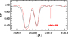 |
Fig. 4 Observed residual flux of the spectrum (solid black line) in the wavelength range of the 313.1 nm Be II resonance doublet, compared to synthetic spectrum (solid red line). The position of the Be II 313.1 nm line is marked with a vertical red line. |
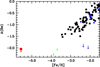 |
Fig. 5 Beryllium abundance in HE 0107−5240 (red symbol) compared to Galactic behaviour data from Boesgaard et al. (2011, black symbols) and Smiljanic et al. (2009, blue symbols), as well as the upper limits for 2MASS J18082002–5104378 and BD+44 493 (Spite et al. 2019, green symbols). |
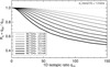 |
Fig. 6 3D correction factor for the 12C/13C isotopic ratio versus the 1D isotopic ratio for different strengths of the 13CH component of the 423.1 nm line pair. A 1D isotopic ratio of 100 with a 13CH equivalent width of 2 mÅ corresponds to a 3D isotopic ratio of ≈90. |
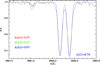 |
Fig. 7 Observed spectra (black line) in the range of the Al I 396.1 nm line, including a tentative detection of Al (red line) and other syntheses (blue and green lines) illustrating the Al line. |
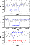 |
Fig. 8 Observed spectra (black line; from top to bottom Fe II 492.3, 501.8, and 516.9 nm), compared to the best fit (red line) and the synthetic profile used to illustrate uncertainty and upper limit (blue line). |
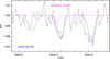 |
Fig. 9 Observed spectra (black line) in the range of the Ba II 455.4 nm line compared to the synthesis of the upper-limit on Ba (pink line), synthesis of the contribution of CH (blue line), and synthesis with CH and the Ba upper limit (red line). |
6 Discussion
HE 0107−5240 is a halo binary system with a prograde Galactic orbit. Its abundances reflect the chemical composition of the cloud from which the system formed. The star belongs to a binary system with an estimated period of about 29 years.
6.1 Stellar chemistry
6.1.1 The carbon isotopic signature: High 13C abundance
Notably, the absolute abundance of 13C in HE 0107−5240, A(13C) = 4.68, exceeds that of nitrogen (A(N) = 4.42) and is second only to oxygen (A(O) = 5.72) and 12C (A(12C) = 6.72), underscoring the significant presence of 13C in the stellar atmosphere.
The carbon isotopic ratio (12C/13C) measured in HE 0107−5240 (also accounting for 3D corrections) is consistent with the value reported by Molaro et al. (2023) and slightly higher than those observed in the sample of unmixed giant stars analysed by Spite et al. (2006).
Nonetheless, the derived ratio remains well below the predictions of zero-metallicity stellar models, which typically yield 12C/13C ratios exceeding 1000 (e.g. Roberti et al. 2024). Ratios in the range 12C/13C = 50–100 can be produced when the hydrogen- and helium-burning shells merge during the presu-pernova evolution of massive stars. This scenario is exemplified by the 25 M⊙ zero-metallicity model with an initial rotational velocity of 300 km s−1 presented by Roberti et al. (2024). Incorporating the nucleosynthetic yields of such models into a Galactic chemical evolution framework, Rizzuti et al. (2025) successfully reproduce observed abundance patterns, provided that H-He shell merging also occurs in stars with metallicities up to [Fe/H] = −3.0. The carbon isotopic ratio observed in HE 0107−5240 also rules out self-pollution from an AGB companion as the origin of its carbon enhancement, as such a process would produce ratios of 12C/13C < 10. Instead, the value is consistent with those found in other unevolved carbon-enhanced metal-poor stars, such as HE 1327−2326 and HE 0233−0343 (see Molaro et al. 2023). It is important to note, however, that measuring isotopic ratios above ∼100 in metal-poor stars is observationally challenging, if not unfeasible. Therefore, published lower limits below this threshold may still be compatible with much higher intrinsic values, potentially exceeding 1000.
6.1.2 Reevaluating NLTE effects: Iron lines show LTE consistency
The LTE iron abundances derived from both neutral and ionised lines in HE 0107−5240 agree perfectly within the uncertainties (as already noted by Christlieb 2008), without applying any corrections, contrary to what NLTE studies typically predict. The Fe II line at 516.9 nm forms at approximately log τ ∼ –1, relatively deep within the stellar atmosphere. Since Fe II is the dominant ionisation state of iron under these conditions, this line is expected to form close to LTE. The agreement between the abundances of Fe I and Fe II implies that the effects of NLTE on Fe I must be small for HE 0107–5240.
This finding contrasts with the literature, where significant positive NLTE corrections are generally reported for neutral iron lines in extremely metal-poor stars (see, e.g. Amarsi et al. 2016; Ezzeddine et al. 2017). For example, Nordlander et al. (2017) investigated 3D-NLTE effects on iron in the ultra-iron-poor star SMSS 0313–6708, which has stellar parameters nearly identical to those of HE 0107−5240; their model was computed specifically for HE 0107−5240. They find a 3D-NLTE correction of approximately +0.8 dex.
If we were to force the Fe II abundance to match the lower Fe I abundance derived by Ezzeddine et al. (2017) under NLTE assumption, we would need to increase the surface gravity of HE 0107−5240 by more than 2 dex, effectively classifying it as a turn-off star. However, this scenario is clearly inconsistent with the Gaia parallax and with the observed profiles of Hα and other Balmer lines, whose wings are too narrow to support such high gravity.
This unexpected result for HE 0107−5240, which is supported by a preliminary consistent result for SMSS J160540.18–144323.1 (Nordlander et al. 2019, discussed in Appendix C), challenges prevailing expectations and highlights the need for further investigation of 1D- and 3D-NLTE effects in the most iron-poor stars.
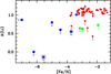 |
Fig. 10 Updated version of Figure 2 from Mucciarelli et al. (2022), using the same symbols: red filled circles indicate normal stars, blue and green filled squares correspond to CEMP stars with ‘low’ and ‘high’ A(C), respectively. HE 0107−5240 is highlighted by a black circle. |
6.1.3 Lithium depletion
According to its stellar parameters, HE 0107−5240 should lie on the Mucciarelli plateau (Mucciarelli et al. 2022), which implies an expected lithium abundance of A(Li) ∼ 1.09. In Fig. 10, we reproduce Figure 2 from Mucciarelli et al. (2022), adding SMSS J1505–1443 (Nordlander et al. 2019) and SDSS J1313–0019 (Allende Prieto et al. 2015), and updating the value for HE 0107−5240. The upper limit on lithium, A(Li) < −0.14, for HE 0107−5240 is consistent with the absence of lithium, suggesting that either the star has destroyed its lithium or it formed from a gas cloud already devoid of lithium.
Several CEMP-no stars fall below the Mucciarelli plateau (see Figure 2 in Mucciarelli et al. 2022), yet some lie on the plateau. For example, Matsuno et al. (2017) measured lithium at the Spite plateau level in two CEMP-no dwarf stars with metal-licities around [Fe/H] ∼ −3.0. This suggests that the nature of their progenitors alone cannot explain the higher incidence of lithium depletion at low metallicities. As discussed in Molaro et al. (2023), the mechanism responsible for lithium depletion appears to correlate more strongly with extremely low iron abundance, rather than with destruction during the evolution of faint supernovae, the likely progenitors of CEMP-no stars.
An alternative explanation is that HE 0107−5240 is an evolved blue straggler, formed through the merger of two lower-mass stars, during which lithium could have been destroyed. Interestingly, the relatively young age we derive for HE 0107−5240 – unusual for a halo star – may support this hypothesis. However, given the large uncertainty in the age estimate, it remains consistent within 1.8σ with an age equal to that of the Universe.
6.1.4 Neutron-capture elements
The new upper limit for barium in HE 0107−5240 satisfies the criterion for classification as a CEMP-no star. In Fig. 11, the star is compared to a sample of EMP stars (excluding CEMP stars) analysed under the LTE assumption by François et al. (2007), showing a comparable [Ba/Fe] ratio. However, a striking contrast is seen with HE 1327–2326, which exhibits a high barium abundance of [Ba/Fe] = +1.0 (Molaro et al. 2023), highlighting the large diversity in neutron-capture element behaviour at low metallicities. In the [Ba/H] versus [Sr/H] plane, HE 0107−5240 is consistent with metal-poor stars (see Fig. 12).
Hansen et al. (2015) propose the existence of a floor in the absolute barium abundance at A(Ba) ∼ − 2.0 for CEMP-no stars. However, HE 0107−5240, with its extremely low [Fe/H] and an upper limit of A(Ba) < −3.87, lies well below this proposed floor and below all upper limits reported in their study (see their Fig. 13). This suggests that either the barium floor occurs at a lower level than previously thought or might not exist at all.
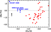 |
Fig. 11 [Ba/Fe] versus [Fe/H] (black arrow) compared to the sample from François et al. (2007) (solid red symbol). Three CEMP stars, HE 1327–2326 (Molaro et al. 2023), SDSSJ 131326.89–001941.4 (Frebel et al. 2015), and HE 0557–4840 (Norris et al. 2007, ApJ, 670, 774), are shown as blue symbols. |
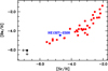 |
Fig. 12 Abundance ratio [Ba/H] versus [Sr/H] (double black arrow) compared to the sample in François et al. (2007) (red full red) and to HE 1327–2326 (Molaro et al. 2023, blue filled circle). |
6.2 Origin of HE 0107−5240
Limongi et al. (2003) proposed a model explaining the observed abundance ratios in HE 0107−5240 by invoking the ejecta of primordial core-collapse supernovae. Specifically, they suggested that elements heavier than Mg were produced in one or more ‘normal’ Population III core-collapse supernovae, whereas the lighter elements originated from enrichment by a failed Pop III supernova – i.e. one leaving behind a very massive remnant. This scenario was based on a detailed analysis of presupernova models and explosive yields presented by Chieffi & Limongi (2002) and Limongi & Chieffi (2002).
In particular, they found that stars with initial masses near 35 M⊙ underwent partial mixing between the He convective shell and the tail of the H shell. This mixing, which is relatively common in zero-metallicity massive stars (see, e.g. Fujimoto et al. 1990; Chieffi et al. 2001; Limongi & Chieffi 2012; Roberti et al. 2024), results in the synthesis of C, N, Na, and Mg in relative proportions consistent with those observed in HE 0107−5240.
A quantitative analysis using these models showed that the observed abundance pattern (specifically C, N, Na, Mg, Ca, Ti, and Ni) could be reproduced by combining the yields of a 15M⊙ ‘normal’ Pop III supernova with those of a 35 M⊙ model in which the mass cut lies within the He shell, corresponding to a remnant mass of 9.4 M⊙ (see Figure 3 in Limongi et al. 2003).
Subsequent spectroscopic studies of HE 0107−5240 enabled the measurement of the [O/Fe] abundance ratio (see Table A.1 for literature values and Table A.2 for our result), which was not available at the time of the original analysis. The measured oxygen abundance, especially the observed [C/O] > 1 ratio, implying a super-solar C/O ratio, presents a potential challenge to the model. This arises because the only region in a massive star where 12C exceeds 16O in abundance is the He convective shell. In this region, incomplete He burning leads to a significant accumulation of 12C prior to its full conversion into 16O.
As shown in the upper panel of Fig. 13, a recent 15 M zerometallicity model (Limongi & Chieffi 2012) exhibits a [C/O] ratio within the He convective shell (between mass coordinates ∼2.2 and ∼3.2 M⊙) compatible with the observed value. Placing the mass cut within this region yields ejecta with a [C/O] ratio in excellent agreement with observations. However, owing to the initial zero metallicity, this region does not produce 14N, which is observed in HE 0107–5240. Hence, while such a mass cut can reproduce the observed [C/O], it does not account for the observed [N/O].
As previously discussed, significant production of 14N and 13C in zero-metallicity stars requires partial mixing between the He convective shell and the overlying H-rich shell. Proton ingestion into the He shell triggers a primary CNO cycle that produces 14N and 13C from freshly synthesised 12C. Although this mixing process is relatively common among zero-metallicity stars, it occurs within a limited mass range, typically between ∼25 and ∼35 M⊙. Proton ingestion also modifies the abundances of 12C and 16O, reducing the [C/O] ratio below that observed in HE 0107−5240.
The bottom panel of Figure 13 shows the internal presuper-nova composition of a 35 M⊙ model (Limongi & Chieffi 2012) in which partial mixing between He and H occurred. In the mixed region of the He shell (mass coordinates ∼11 to ∼20 M⊙), the [C/O] ratio drops significantly, while [N/O] rises above the observed value. Conversely, in the deeper unmixed region of the He shell (between ∼8.5 and ∼11 M⊙)12 C dominates over 16O, resulting in a high [C/O] and low [N/O], along with [Na/O] and [Mg/O] values slightly below those observed. These abundance patterns depend on the extent of He burning in the inner shell and the efficiency and depth of mixing with the H-rich envelope.
Among the models presented by Limongi & Chieffi (2012), this distinctive internal structure is found only in the 35 M⊙ case. However, due to the limited mass resolution of the available grid, it is currently not possible to fully explore how this behaviour changes with initial stellar mass. It remains plausible that models with intermediate or different initial masses could yield C, N, O, Na, and Mg abundance ratios more consistent with the observations. To investigate this hypothesis, we plan to conduct a more extensive and fine-sampled study in future work.
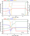 |
Fig. 13 Abundance ratios of C,N, Na, and Mg/O as a function of remnant mass for a zero-metallicity 15 M⊙ (top) and 35 M⊙ (bottom) star (Limongi & Chieffi 2012) after the explosion (bold sold lines, left y-axis). The abundance ratio X/O is defined as the difference between the predicted and observed [X/O] values. The right y-axis shows postexplosion interior profiles of 4He (dotted black line), 12C (red), 16O (cyan), 23Na (blue), and 24Mg (orange). |
7 Conclusions
The main conclusions of this study are:
Observations of HE 0107−5240 over a longer temporal baseline have refined the orbital period to
 , which is smaller than previously derived (Aguado et al. 2022).
The binary system follows a halo prograde orbit around the Galactic centre;
New stringent upper limits on Sr and Ba abundances confirm that HE 0107−5240 satisfies the CEMP-no classification. These limits do not support the existence of a floor in the absolute barium abundance at A(Ba) ∼ −2.0 for CEMP-no stars, as proposed by Hansen et al. (2015);
Lithium remains undetected, at levels much lower than those reported by Mucciarelli et al. (2022) for giant stars, implying that Li has been depleted either within the star itself or in its progenitor;
The Fe abundances derived under LTE assumptions from both Fe I and Fe II lines are in good agreement, calling into question the reliability of published NLTE corrections for Fe I;
The 12C/13C isotopic ratio is measured to be 110±12, which is close to the solar value. This ratio is sensitive to 3D NLTE effects, which tend to decrease the derived value. The NLTE-corrected ratio is 87, higher than the average value observed in unmixed stars by Spite et al. (2006), yet still low enough for 13C to remain the third most abundant element in the stellar atmosphere.
Acknowledgements
PB acknowledges support from the ERC advanced grant N. 835087 – SPIAKID. LM gratefully acknowledges support from ANID-FONDECYT Regular Project n. 1251809. This work has made use of data from the European Space Agency (ESA) mission Gaia (https://www.cosmos.esa.int/gaia), processed by the Gaia Data Processing and Analysis Consortium (DPAC, https://www.cosmos.esa.int/web/gaia/dpac/consortium). Funding for the DPAC has been provided by national institutions, in particular the institutions participating in the Gaia Multilateral Agreement. JIGH, DSA, RR and CAP acknowledge financial support from the Spanish Ministry of Science, Innovation and Universities (MICIU) projects PID2020-117493GB-I00 and PID2023-149982NB-I00. This research has made use of the SIMBAD database, operated at CDS, Strasbourg, France. PM warmly acknowledge Richard Hoppe for stressing the importance of the 3D/NLTE effects on the carbon isotopic ratio. NCS acknowledges funding by the European Union (ERC, FIERCE, 101052347). Views and opinions expressed are however those of the author(s) only and do not necessarily reflect those of the European Union or the European Research Council. Neither the European Union nor the granting authority can be held responsible for them. NJN was supported by FCT – Fundação para a Ciência e a Tecnologia through national funds by grants UIDB/04434/2020 and UIDP/04434/2020. The work of CJAPM was financed by Portuguese funds through FCT (Fundação para a Ciência e a Tecnologia) in the framework of the project 2022.04048.PTDC (Phi in the Sky, DOI 10.54499/2022.04048.PTDC). CJM also acknowledges FCT and POCH/FSE (EC) support through Investigador FCT Contract 2021.01214.CEECIND/CP1658/CT0001 (DOI 10.54499/2021.01214.CEECIND/CP1658/CT0001). MTM acknowledges the support of the Australian Research Council through Future Fellowship grant FT180100194 and through the Australian Research Council Centre of Excellence in Optical Microcombs for Breakthrough Science (project number CE230100006) funded by the Australian Government.
References
- Aguado, D. S., Molaro, P., Caffau, E., et al. 2022, A&A, 668, A86 [NASA ADS] [CrossRef] [EDP Sciences] [Google Scholar]
- Allende Prieto, C., Fernández-Alvar, E., Aguado, D. S., et al. 2015, A&A, 579, A98 [NASA ADS] [CrossRef] [EDP Sciences] [Google Scholar]
- Amarsi, A. M., Lind, K., Asplund, M., Barklem, P. S., & Collet, R. 2016, MNRAS, 463, 1518 [NASA ADS] [CrossRef] [Google Scholar]
- Andrievsky, S. M., Spite, M., Korotin, S. A., et al. 2007, A&A, 464, 1081 [NASA ADS] [CrossRef] [EDP Sciences] [Google Scholar]
- Andrievsky, S. M., Spite, M., Korotin, S. A., et al. 2008, A&A, 481, 481 [NASA ADS] [CrossRef] [EDP Sciences] [Google Scholar]
- Andrievsky, S. M., Spite, M., Korotin, S. A., et al. 2010, A&A, 509, A88 [NASA ADS] [CrossRef] [EDP Sciences] [Google Scholar]
- Andrievsky, S. M., Spite, F., Korotin, S. A., et al. 2011, A&A, 530, A105 [CrossRef] [EDP Sciences] [Google Scholar]
- Arentsen, A., Starkenburg, E., Shetrone, M. D., et al. 2019, A&A, 621, A108 [NASA ADS] [CrossRef] [EDP Sciences] [Google Scholar]
- Beers, T. C., & Christlieb, N. 2005, ARA&A, 43, 531 [NASA ADS] [CrossRef] [Google Scholar]
- Beers, T. C., Preston, G. W., & Shectman, S. A. 1992, AJ, 103, 1987 [NASA ADS] [CrossRef] [Google Scholar]
- Bensby, T., Feltzing, S., & Oey, M. S. 2014, A&A, 562, A71 [NASA ADS] [CrossRef] [EDP Sciences] [Google Scholar]
- Bergemann, M., & Gehren, T. 2008, A&A, 492, 823 [NASA ADS] [CrossRef] [EDP Sciences] [Google Scholar]
- Bessell, M. S., Christlieb, N., & Gustafsson, B. 2004, ApJ, 612, L61 [NASA ADS] [CrossRef] [Google Scholar]
- Boesgaard, A. M., Rich, J. A., Levesque, E. M., & Bowler, B. P. 2011, ApJ, 743, 140 [Google Scholar]
- Bonifacio, P., Molaro, P., Beers, T. C., & Vladilo, G. 1998, A&A, 332, 672 [NASA ADS] [Google Scholar]
- Bonifacio, P., Caffau, E., Spite, M., et al. 2015, A&A, 579, A28 [NASA ADS] [CrossRef] [EDP Sciences] [Google Scholar]
- Bonifacio, P., Caffau, E., Ludwig, H. G., et al. 2018, A&A, 611, A68 [NASA ADS] [CrossRef] [EDP Sciences] [Google Scholar]
- Bonifacio, P., Molaro, P., Adibekyan, V., et al. 2020, A&A, 633, A129 [NASA ADS] [CrossRef] [EDP Sciences] [Google Scholar]
- Bonifacio, P., Monaco, L., Salvadori, S., et al. 2021, A&A, 651, A79 [NASA ADS] [CrossRef] [EDP Sciences] [Google Scholar]
- Bovy, J. 2015, ApJS, 216, 29 [NASA ADS] [CrossRef] [Google Scholar]
- Bovy, J., Allende Prieto, C., Beers, T. C., et al. 2012, ApJ, 759, 131 [NASA ADS] [CrossRef] [Google Scholar]
- Caffau, E., Bonifacio, P., François, P., et al. 2011a, Nature, 477, 67 [NASA ADS] [CrossRef] [Google Scholar]
- Caffau, E., Ludwig, H. G., Steffen, M., Freytag, B., & Bonifacio, P. 2011b, Sol. Phys., 268, 255 [Google Scholar]
- Caffau, E., Bonifacio, P., Monaco, L., et al. 2024a, A&A, 684, L4 [NASA ADS] [CrossRef] [EDP Sciences] [Google Scholar]
- Caffau, E., Bonifacio, P., Monaco, L., et al. 2024b, A&A, 691, A245 [NASA ADS] [CrossRef] [EDP Sciences] [Google Scholar]
- Caffau, E., Katz, D., Bonifacio, P., et al. 2025, Astron. Nachr., 346, e70025 [Google Scholar]
- Cayrel, R. 1988, in The Impact of Very High S/N Spectroscopy on Stellar Physics, 132, eds. G. Cayrel de Strobel, & M. Spite, 345 [Google Scholar]
- Cayrel, R., Depagne, E., Spite, M., et al. 2004, A&A, 416, 1117 [NASA ADS] [CrossRef] [EDP Sciences] [Google Scholar]
- Chamberlain, J. W., & Aller, L. H. 1951, ApJ, 114, 52 [NASA ADS] [CrossRef] [Google Scholar]
- Chieffi, A., & Limongi, M. 2002, ApJ, 577, 281 [NASA ADS] [CrossRef] [Google Scholar]
- Chieffi, A., Domínguez, I., Limongi, M., & Straniero, O. 2001, ApJ, 554, 1159 [Google Scholar]
- Christlieb, N. 2008, Phys. Scr. Vol. T, 133, 014034 [Google Scholar]
- Christlieb, N., Bessell, M. S., Beers, T. C., et al. 2002, Nature, 419, 904 [NASA ADS] [CrossRef] [PubMed] [Google Scholar]
- Christlieb, N., Gustafsson, B., Korn, A. J., et al. 2004, ApJ, 603, 708 [NASA ADS] [CrossRef] [Google Scholar]
- Collet, R., Asplund, M., & Trampedach, R. 2006, ApJ, 644, L121 [NASA ADS] [CrossRef] [Google Scholar]
- Collet, R., Hayek, W., Asplund, M., et al. 2011, A&A, 528, A32 [NASA ADS] [CrossRef] [EDP Sciences] [Google Scholar]
- Ezzeddine, R., Frebel, A., & Plez, B. 2017, ApJ, 847, 142 [Google Scholar]
- Fernando, A. M., Bernath, P. F., Hodges, J. N., & Masseron, T. 2018, J. Quant. Spec. Radiat. Transf., 217, 29 [NASA ADS] [CrossRef] [Google Scholar]
- Feuillet, D. K., Sahlholdt, C. L., Feltzing, S., & Casagrande, L. 2021, MNRAS, 508, 1489 [NASA ADS] [CrossRef] [Google Scholar]
- Foreman-Mackey, D., Agol, E., Ambikasaran, S., & Angus, R. 2017, AJ, 154, 220 [Google Scholar]
- François, P., Depagne, E., Hill, V., et al. 2007, A&A, 476, 935 [Google Scholar]
- Frebel, A., Chiti, A., Ji, A. P., et al. 2015, ApJ, 810, L27 [NASA ADS] [CrossRef] [Google Scholar]
- Freytag, B., Steffen, M., Ludwig, H. G., et al. 2012, J. Computat. Phys., 231, 919 [NASA ADS] [CrossRef] [Google Scholar]
- Fujimoto, M. Y., Iben, I.Jr., & Hollowell, D. 1990, ApJ, 349, 580 [CrossRef] [Google Scholar]
- Fulton, B. J., Petigura, E. A., Blunt, S., & Sinukoff, E. 2018, PASP, 130, 044504 [Google Scholar]
- Gaia Collaboration (Vallenari, A., et al.) 2023, A&A, 674, A1 [NASA ADS] [CrossRef] [EDP Sciences] [Google Scholar]
- Gallagher, A. J., Caffau, E., Bonifacio, P., et al. 2017, A&A, 598, L10 [NASA ADS] [CrossRef] [EDP Sciences] [Google Scholar]
- Hansen, T., Hansen, C. J., Christlieb, N., et al. 2015, ApJ, 807, 173 [Google Scholar]
- Jedamzik, K., & Rehm, J. B. 2001, Phys. Rev. D, 64, 023510 [Google Scholar]
- Kurucz, R. L. 2005, Mem. Soc. Astron. Ital. Suppl., 8, 14 [Google Scholar]
- Kučinskas, A., Klevas, J., Ludwig, H. G., et al. 2018, A&A, 613, A24 [NASA ADS] [CrossRef] [EDP Sciences] [Google Scholar]
- Lardo, C., Mashonkina, L., Jablonka, P., et al. 2021, MNRAS, 508, 3068 [NASA ADS] [CrossRef] [Google Scholar]
- Lebreton, Y., & Reese, D. R. 2020, A&A, 642, A88 [NASA ADS] [CrossRef] [EDP Sciences] [Google Scholar]
- Limberg, G., Placco, V. M., Ji, A. P., et al. 2025, ApJ, 989, L18 [Google Scholar]
- Limongi, M., & Chieffi, A. 2002, PASA, 19, 246 [Google Scholar]
- Limongi, M., & Chieffi, A. 2012, ApJS, 199, 38 [NASA ADS] [CrossRef] [Google Scholar]
- Limongi, M., Chieffi, A., & Bonifacio, P. 2003, ApJ, 594, L123 [CrossRef] [Google Scholar]
- Lindegren, L., Bastian, U., Biermann, M., et al. 2021, A&A, 649, A4 [EDP Sciences] [Google Scholar]
- Lodders, K., Palme, H., & Gail, H. P. 2009, Landolt Börnstein, 4B, 712 [Google Scholar]
- Ludwig, H.-G., & Steffen, M. 2012, in Astrophysics and Space Science Proceedings, 26, Red Giants as Probes of the Structure and Evolution of the Milky Way, eds. A. Miglio, J. Montalbán, & A. Noels, 125 [Google Scholar]
- Ludwig, H. G., & Steffen, M. 2013, Mem. Soc. Astron. Ital. Suppl., 24, 53 [Google Scholar]
- Malaney, R. A., & Fowler, W. A. 1989, ApJ, 345, L5 [Google Scholar]
- Manchon, L., Deal, M., Goupil, M. J., et al. 2024, A&A, 687, A146 [NASA ADS] [CrossRef] [EDP Sciences] [Google Scholar]
- Matsuno, T., Aoki, W., Beers, T. C., Lee, Y. S., & Honda, S. 2017, AJ, 154, 52 [NASA ADS] [CrossRef] [Google Scholar]
- Meléndez, J., & Barbuy, B. 2009, A&A, 497, 611 [NASA ADS] [CrossRef] [EDP Sciences] [Google Scholar]
- Molaro, P., Aguado, D. S., Caffau, E., et al. 2023, A&A, 679, A72 [NASA ADS] [CrossRef] [EDP Sciences] [Google Scholar]
- Mucciarelli, A., Monaco, L., Bonifacio, P., et al. 2022, A&A, 661, A153 [NASA ADS] [CrossRef] [EDP Sciences] [Google Scholar]
- Nakamura, R., & Hashimoto, M.-A. 2017, in 14th International Symposium on Nuclei in the Cosmos (NIC2016), eds. S. Kubono, T. Kajino, S. Nishimura, T. Isobe, S. Nagataki, T. Shima, & Y. Takeda, 020108 [Google Scholar]
- Nave, G., & Johansson, S. 2013, ApJS, 204, 1 [NASA ADS] [CrossRef] [Google Scholar]
- Nordlander, T., Amarsi, A. M., Lind, K., et al. 2017, A&A, 597, A6 [NASA ADS] [CrossRef] [EDP Sciences] [Google Scholar]
- Nordlander, T., Bessell, M. S., Da Costa, G. S., et al. 2019, MNRAS, 488, L109 [Google Scholar]
- Norris, J. E., Ryan, S. G., & Beers, T. C. 1997, ApJ, 489, L169 [NASA ADS] [CrossRef] [Google Scholar]
- Norris, J. E., Christlieb, N., Korn, A. J., et al. 2007, ApJ, 670, 774 [NASA ADS] [CrossRef] [Google Scholar]
- Pietrinferni, A., Cassisi, S., Salaris, M., & Castelli, F. 2006, ApJ, 642, 797 [Google Scholar]
- Pietrinferni, A., Hidalgo, S., Cassisi, S., et al. 2021, ApJ, 908, 102 [NASA ADS] [CrossRef] [Google Scholar]
- Planck Collaboration VI. 2020, A&A, 641, A6 [NASA ADS] [CrossRef] [EDP Sciences] [Google Scholar]
- Prakapavičius, D., Kučinskas, A., Dobrovolskas, V., et al. 2017, A&A, 599, A128 [NASA ADS] [CrossRef] [EDP Sciences] [Google Scholar]
- Reese, D. R., & Lebreton, Y. 2020, SPInS: Stellar Parameters INferred Systematically, Astrophysics Source Code Library [record ascl:2009.006] [Google Scholar]
- Rizzuti, F., Cescutti, G., Molaro, P., et al. 2025, A&A, 698, A118 [NASA ADS] [CrossRef] [EDP Sciences] [Google Scholar]
- Roberti, L., Limongi, M., & Chieffi, A. 2024, ApJS, 270, 28 [NASA ADS] [CrossRef] [Google Scholar]
- Schlafly, E. F., & Finkbeiner, D. P. 2011, ApJ, 737, 103 [Google Scholar]
- Schnabel, R., Schultz-Johanning, M., & Kock, M. 2004, A&A, 414, 1169 [NASA ADS] [CrossRef] [EDP Sciences] [Google Scholar]
- Schönrich, R., Binney, J., & Dehnen, W. 2010, MNRAS, 403, 1829 [NASA ADS] [CrossRef] [Google Scholar]
- Sestito, F., Longeard, N., Martin, N. F., et al. 2019, MNRAS, 484, 2166 [NASA ADS] [CrossRef] [Google Scholar]
- Sitnova, T. M., Mashonkina, L. I., Ezzeddine, R., & Frebel, A. 2019, MNRAS, 485, 3527 [NASA ADS] [CrossRef] [Google Scholar]
- Smiljanic, R., Pasquini, L., Bonifacio, P., et al. 2009, A&A, 499, 103 [NASA ADS] [CrossRef] [EDP Sciences] [Google Scholar]
- Speagle, J. S. 2020, MNRAS, 493, 3132 [Google Scholar]
- Spite, M., Bonifacio, P., Spite, F., et al. 2019, A&A, 624, A44 [NASA ADS] [CrossRef] [EDP Sciences] [Google Scholar]
- Spite, M., Cayrel, R., Hill, V., et al. 2006, A&A, 455, 291 [NASA ADS] [CrossRef] [EDP Sciences] [Google Scholar]
- Starkenburg, E., Aguado, D. S., Bonifacio, P., et al. 2018, MNRAS, 481, 3838 [NASA ADS] [CrossRef] [Google Scholar]
- Takeda, Y., Hashimoto, O., Taguchi, H., et al. 2005, PASJ, 57, 751 [NASA ADS] [Google Scholar]
- Tauris, T. M., & van den Heuvel, E. P. J. 2006, in Compact Stellar X-ray Sources, 39, 623 [NASA ADS] [CrossRef] [Google Scholar]
- Thomas, D., Schramm, D. N., Olive, K. A., et al. 1994, ApJ, 430, 291 [Google Scholar]
- Yong, D., Norris, J. E., Bessell, M. S., et al. 2013, ApJ, 762, 26 [Google Scholar]
Echelle SPectrograph for Rocky Exoplanets and Stable Spectroscopic Observations.
Southern African Large Telescope High Resolution Spectrograph.
Note that there is a typo in Table 2 of Aguado et al. (2022); the epoch 9618.061 should read 9518.061.
RADVEL is a Python package for the modelling of radial velocity time-series data, available at https://radvel.readthedocs.io/en/latest/index.html
CELERITE is a library for fast and scalable Gaussian-process (GP) regression in one dimension, available in https://celerite.readthedocs.io/en/stable/
DYNESTY is a pure-Python, MIT-licenced dynamic nested-sampling package for estimating Bayesian posteriors and evidences, available at https://dynesty.readthedocs.io/en/stable/
Mucciarelli et al., accepted, and references therein https://sites.google.com/view/koala-database/
 .
.
This is in stark contrast to the 3D temperature structure of SDSS J102915.14+172927.9, one of the most metal-poor star known to date, where horizontal temperature fluctuations are effectively suppressed (see Caffau et al. 2024b, Figure 2).
Appendix A Data from the literature
The abundances and upper limits derived in the literature are reported in Table A.1, while in Table A.2 our results are listed.
Appendix B Model atmospheres and spectrum synthesis
B.1 1D (LTE) models and spectrum synthesis
As 1D model atmosphere we computed an ATLAS 9 (Kurucz 2005) model with Teff= 5100 K and log g 2.2, with metallicity [M/H]=−5.0, α enhancement +0.4 dex and microturbulence 1.0 kms−1, using the Opacity Distribution Function of Mucciarelli et al. (A&A accepted). The effect of microturbulence on the model structure and emerging flux is minor (see Kučinskas et al. 2018). The ODF used assumes the (scaled) solar abundances of Caffau et al. (2011b) and Lodders et al. (2009) for the elements not included in the former paper. This is also the set of solar abundances assumed elsewhere in this work.
We also computed an ATLAS 12 model atmosphere with the precise chemical composition of HE 0107−5240. We verified that the ATLAS 9 and ATLAS 12 models have exactly the same temperature structure for all layers that are relevant for the line formation. The two models begin to differ for log(τRoss) < −4, the ATLAS 12 model being cooler. This difference is not due to the different chemical composition but is due to the different temperature correction algorithm in the two codes. One should bear in mind that real stars are expected to show a chromospheric temperature rise at very low optical depths that cannot be modelled by the 1D LTE approach of the ATLAS codes. We typically compute models up to optical depth of log(τRoss) ∼− 6.5 just to avoid an edge effect when computing the cores of strong lines. We do not claim that these are correctly computed, since they certainly are sensitive to the structure of the chromosphere and NLTE effects.
When computing the ATLAS models we used the default control card SCATTERING ON that includes the scattering term in the computation of the continuum source function. The effect of scattering is discussed in Bonifacio et al. (2018, section 2.3).
To compute the synthetic spectra from our 1D model atmosphere we used the SYNTHE suite (Kurucz 2005). The scattering is treated explicitly and without approximation. In fact, this is specially important in the UV range: if one does not treat scattering explicitly one finds a trend of abundances with wavelength (see Cayrel et al. 2004, section 3.2 for a discussion).
B.2 3D (LTE) models and abundance corrections
Two dedicated high-resolution CO5BOLD models (288×288×200 grid) have been computed to represent the dynamic atmosphere of HE 0107–5240 (Teff ∼ 5100 K, log g = 2.2). For the first model, we assumed [M/H]= −4.0 solar scaled abundances (with an α enhancement of +0.4 dex), for the second one an enhancement of C and N by 3.0 dex and of O by 2.6 dex was applied with respect to the first model. The detailed chemical composition is relevant for constructing the 14-band opacity tables used for computing the radiation transport in CO5BOLD. Continuum scattering is treated approximately by ignoring the scattering opacity in the optically thin layers as suggested by Collet et al. (2011), (see also Ludwig & Steffen 2012, 2013).
As shown in Fig. B.1, both models are characterised by substantial photospheric temperature fluctuations that cannot be captured by 1D (or 3D-averaged) models.11 Spectral lines emerging from an inhomogeneous atmosphere can have a significantly different strength (and shape) compared to the same lines formed in a representative 1D (<3D>) atmosphere. In the present case, the investigated CH, NH, OH molecular lines show a highly non-linear temperature dependence. The strong temperature fluctuations in the 3D models lead to a substantial enhancement of these lines, so that the abundances derived from these models are significantly lower than those obtained from a standard 1D analysis.
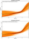 |
Fig. B.1 3D versus 1D temperature structure of two 3D CO5BOLD models representing HE 0107–5240 (Teff ∼ 5090 K, log g = 2.2, [M/H]=−4.0, α enhancement +0.4), assuming different CNO abundances for computing the opacity tables: Top: A(C)=4.39, A (N)=3.78, A(O)=5.06; Bottom: A(C)=7.39, A(N)=6.78, A(O)=7.66. The orange band outlines the 3D temperature distribution constructed from 20 snapshots of the respective high-resolution model, each resampled to 144 × 144 × 200 grid points. The dashed blue lines enclose 95.5% of the data points at given Rosseland optical depth. The black solid line shows the <3D> model (the temperature of the 3D model averaged at constant τRoss), the black long-dashed line represents the T(τRoss) relation of the 1D LHD reference model atmosphere with identical stellar parameters, treating convection by standard mixing-length theory, but otherwise using the same input physics as the 3D hydrodynamical model. |
We use the line formation code Linfor3D12 to compute synthetic spectra from selected snapshots of the 3D hydrodynamical model as well as from the 1D LHD reference model atmosphere with identical stellar parameters and input physics as the 3D hydrodynamical model, except that convection is treated by the mixing-length theory. Linfor3D treats continuum scattering as true absorption which may compromise the synthetic spectra in the UV, e.g. of the OH lines near 319.5 nm. However, the abundance corrections are probably affected only marginally since the same scattering approximation is used for the line formation in the 3D and the 1D LHD models.
Abundances from the literature.
3D abundance corrections are derived for individual spectral lines from a comparison of 3D and 1D equivalent widths. More specifically, if the observed equivalent width of a spectral line of element X is reproduced with (logarithmic) abundance A3D(X) based on the 3D model and with A1D(X) when using the 1D model, the 3D abundance correction is defined as ∆3D = A3D(X) − A1D(X). For the molecular lines and the Fe II line investigated in this work, both 3D and 1D line formation are treated in LTE.
It must be noted that the 3D abundance correction of partly saturated lines depends on the microturbulence velocity assumed in the 1D spectrum synthesis. Here we have determined the optimal value of the microturbulence as 1.3 km s−1 from a curve-of-growth analysis of the Fe II line at 516.9 nm.
In the present work, the 12C/13C isotopic ratio is derived from the CH lines in the G-band where the 12CH and the 13CH lines are well separated such that their individual equivalent widths can be measured. We can therefore compute individual 3D abundance corrections,  and
and  for both isotopic components as described above. The isotopic ratio derived in 3D, q3D, is related to the 1D isotopic ratio, q1D, by
  . If the corrections for both components are identical, the 3D correction factor for the isotopic ratio is Rq = q3D/q1D = 1.
As mentioned in Sect. 5.3, the magnitude of the 3D corrections depends on the chemical composition, in particular the CNO abundances, adopted for the construction of the 3D atmosphere and the 1D reference model. This is because the molecular opacities influence the resulting temperature structure, as demonstrated in Fig. B.1. The model with the lower CNO abundances (model A, top panel) shows a T-distribution that is strongly biased towards the lowest temperatures, visible as the dark-orange band in the upper photosphere, which leads to a plateau in the <3D> temperature profile around log τRoss ∼ −4. In the model with enhanced CNO abundances (model B, bottom), the T-distribution is more symmetric, and the <3D> and 1D T(τ) relations are more similar throughout the photosphere.
Abundances derived in this work.
The physical reasons for these differences need yet to be understood. For a given carbon abundance, model A produces stronger CH lines due to the excess of cool temperatures. It appears plausible that the larger asymmetry of the T-distribution and the larger separation between <3D> and 1D reference model lead to larger (more negative) 3D abundance corrections for the molecular lines in model A than in model B. Since the 3D and 1D curves-of-growth are running almost parallel in model B, the correction factor for the isotopic ratio is close to 1, while it is significantly below 1 in model A.
Reliable 3D corrections can only be evaluated when a new 3D model is available that is based on a (yet unavailable) custom-made opacity table representative of the actual chemical composition of HE 0107–5240.
Appendix C Ionised Fe in SMSS J160540.18–144323.1
The problem, discussed in Sect. 6.1.2, about the large NLTE corrections for HE 0107−5240 proposed in the literature for A(Fe) from Fe I lines (see Ezzeddine et al. 2017; Nordlander et al. 2017) and that bring tension with A(Fe) from Fe II lines, is also true for SMSS J160540.18–144323.1 (Nordlander et al. 2019). We took the advantage of 18 ESPRESSO observations to investigate the Fe II line at 516.9 nm, the same one investigated in HE 0107−5240 and shown in the lower panel of Fig. 8. We here suppose that the NLTE correction for Fe II line is negligible for this star as for HE 0107−5240. In Fig. C.1 the observed spectrum of SMSS J160540.18–144323.1 (solid black) is compared to a synthesis (solid blue) with the LTE iron abundance derived from neutral Fe lines (A(Fe)=1.24 Nordlander et al. 2019): the agreement observation/synthesis is good for both the Fe I and the Fe II line, which is not detected. A NLTE correction of +0.2 dex in Fe I (a value compatible with the NLTE correction for a more metal rich model derived in the MPIA database and discussed in Sect. 5.3) would bring A(Fe)=1.44: the solid green synthesis in the figure shows that the profile is compatible with the observations of the Fe II line. The ‘large’ NLTE correction on Fe I (as suggested by Nordlander et al. 2017; Ezzeddine et al. 2017) is not compatible with the observation. A NLTE correction of +0.8 dex would bring the LTE A(Fe) value at 2.04, and this is shown as a red solid profile in the figure. Clearly such a NLTE correction would imply the Fe II line to be visible at this observation quality, and this is not the case. A dedicated work will perform a careful investigation of this line as well as a complete analysis of this ESPRESSO spectrum.
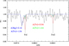 |
Fig. C.1 Observed spectra (solid black) of SMSS J160540.18–144323.1, compared to 1D-LTE synthesis with different A(Fe) values (solid blue, green and red). |
All Tables
Revised orbital parameters of HE 0107−5240 derived using a Markov chain Monte Carlo (MCMC) analysis.
All Figures
|
Fig. 1 Top panels: position of HE 0107−5240 (filled black star) in the Toomre diagram (left) and the orbital energy versus angular momentum (right). Bottom panels: square root of the radial action versus the azimuthal action (left) and action diamond (right). Coloured points represent stars from the good-parallax sample of Bonifacio et al. (2021). The red and green shaded areas indicate the regions defined by Feuillet et al. (2021) to select candidate Gaia-Sausage-Enceladus (GSE) and Sequoia stars. |
| In the text | |
|
Fig. 2 Radial velocities (RV) of HE 0107−5240 versus heliocentric Julian date (HJD), together with the best-fit RV model. The inset within the middle panel shows ESPRESSO RV points after subtracting the best-fit model. The root mean square (RMS) of all residuals is indicated in the middle panel, while the RMS values from each spectrograph are given in the bottom panels. |
| In the text | |
|
Fig. 3 Isochrones from the BASTI database (Pietrinferni et al. 2021) in a Gaia colour-magnitude diagram. The two green points correspond to HE 0107−5240, assuming surface gravities of log g = 2.20 (upper point) and 2.46 (lower point), respectively. |
| In the text | |
|
Fig. 4 Observed residual flux of the spectrum (solid black line) in the wavelength range of the 313.1 nm Be II resonance doublet, compared to synthetic spectrum (solid red line). The position of the Be II 313.1 nm line is marked with a vertical red line. |
| In the text | |
|
Fig. 5 Beryllium abundance in HE 0107−5240 (red symbol) compared to Galactic behaviour data from Boesgaard et al. (2011, black symbols) and Smiljanic et al. (2009, blue symbols), as well as the upper limits for 2MASS J18082002–5104378 and BD+44 493 (Spite et al. 2019, green symbols). |
| In the text | |
|
Fig. 6 3D correction factor for the 12C/13C isotopic ratio versus the 1D isotopic ratio for different strengths of the 13CH component of the 423.1 nm line pair. A 1D isotopic ratio of 100 with a 13CH equivalent width of 2 mÅ corresponds to a 3D isotopic ratio of ≈90. |
| In the text | |
|
Fig. 7 Observed spectra (black line) in the range of the Al I 396.1 nm line, including a tentative detection of Al (red line) and other syntheses (blue and green lines) illustrating the Al line. |
| In the text | |
|
Fig. 8 Observed spectra (black line; from top to bottom Fe II 492.3, 501.8, and 516.9 nm), compared to the best fit (red line) and the synthetic profile used to illustrate uncertainty and upper limit (blue line). |
| In the text | |
|
Fig. 9 Observed spectra (black line) in the range of the Ba II 455.4 nm line compared to the synthesis of the upper-limit on Ba (pink line), synthesis of the contribution of CH (blue line), and synthesis with CH and the Ba upper limit (red line). |
| In the text | |
|
Fig. 10 Updated version of Figure 2 from Mucciarelli et al. (2022), using the same symbols: red filled circles indicate normal stars, blue and green filled squares correspond to CEMP stars with ‘low’ and ‘high’ A(C), respectively. HE 0107−5240 is highlighted by a black circle. |
| In the text | |
|
Fig. 11 [Ba/Fe] versus [Fe/H] (black arrow) compared to the sample from François et al. (2007) (solid red symbol). Three CEMP stars, HE 1327–2326 (Molaro et al. 2023), SDSSJ 131326.89–001941.4 (Frebel et al. 2015), and HE 0557–4840 (Norris et al. 2007, ApJ, 670, 774), are shown as blue symbols. |
| In the text | |
|
Fig. 12 Abundance ratio [Ba/H] versus [Sr/H] (double black arrow) compared to the sample in François et al. (2007) (red full red) and to HE 1327–2326 (Molaro et al. 2023, blue filled circle). |
| In the text | |
|
Fig. 13 Abundance ratios of C,N, Na, and Mg/O as a function of remnant mass for a zero-metallicity 15 M⊙ (top) and 35 M⊙ (bottom) star (Limongi & Chieffi 2012) after the explosion (bold sold lines, left y-axis). The abundance ratio X/O is defined as the difference between the predicted and observed [X/O] values. The right y-axis shows postexplosion interior profiles of 4He (dotted black line), 12C (red), 16O (cyan), 23Na (blue), and 24Mg (orange). |
| In the text | |
|
Fig. B.1 3D versus 1D temperature structure of two 3D CO5BOLD models representing HE 0107–5240 (Teff ∼ 5090 K, log g = 2.2, [M/H]=−4.0, α enhancement +0.4), assuming different CNO abundances for computing the opacity tables: Top: A(C)=4.39, A (N)=3.78, A(O)=5.06; Bottom: A(C)=7.39, A(N)=6.78, A(O)=7.66. The orange band outlines the 3D temperature distribution constructed from 20 snapshots of the respective high-resolution model, each resampled to 144 × 144 × 200 grid points. The dashed blue lines enclose 95.5% of the data points at given Rosseland optical depth. The black solid line shows the <3D> model (the temperature of the 3D model averaged at constant τRoss), the black long-dashed line represents the T(τRoss) relation of the 1D LHD reference model atmosphere with identical stellar parameters, treating convection by standard mixing-length theory, but otherwise using the same input physics as the 3D hydrodynamical model. |
| In the text | |
|
Fig. C.1 Observed spectra (solid black) of SMSS J160540.18–144323.1, compared to 1D-LTE synthesis with different A(Fe) values (solid blue, green and red). |
| In the text | |
Current usage metrics show cumulative count of Article Views (full-text article views including HTML views, PDF and ePub downloads, according to the available data) and Abstracts Views on Vision4Press platform.
Data correspond to usage on the plateform after 2015. The current usage metrics is available 48-96 hours after online publication and is updated daily on week days.
Initial download of the metrics may take a while.