| Issue |
A&A
Volume 704, December 2025
|
|
|---|---|---|
| Article Number | A282 | |
| Number of page(s) | 19 | |
| Section | Stellar atmospheres | |
| DOI | https://doi.org/10.1051/0004-6361/202556947 | |
| Published online | 17 December 2025 | |
The R-Process Alliance: Exploring the cosmic scatter among ten r-process sites with stellar abundances★
1
Astronomy department, Stockholm University,
Roslagstullsbacken 21,
114 21
Stockholm,
Sweden
2
Department of Physics, North Carolina State University,
2401 Stinson Dr, Box 8202,
Raleigh,
NC
27695,
USA
3
Joint Institute for Nuclear Astrophysics – Center for the Evolution of the Elements (JINA-CEE),
USA
4
NSF NOIRLab,
Tucson,
AZ
85719,
USA
5
Department of Physics and Kavli Institute for Astrophysics and Space Research, Massachusetts Institute of Technology,
Cambridge,
MA
02139,
USA
6
Department of Physics and Astronomy, University of Notre Dame,
Notre Dame,
IN
46556,
USA
7
Department of Astronomy, University of Florida, Bryant Space Science Center,
Gainesville,
FL
32611,
USA
8
Lawrence Livermore National Laboratory,
7000 East Avenue,
Livermore,
CA
94550,
USA
9
Department of Physics and Astronomy, San Francisco State University,
San Francisco,
CA
94132,
USA
10
Institute of Astronomy, University of Cambridge,
Madingley Rd,
Cambridge
CB3 0HA,
UK
11
Observatories of the Carnegie Institution for Science,
813 Santa Barbara St.,
Pasadena,
CA
91101,
USA
12
Department of Astronomy and McDonald Observatory, The University of Texas,
Austin,
TX
78712,
USA
★★ Corresponding author: This email address is being protected from spambots. You need JavaScript enabled to view it.
Received:
22
August
2025
Accepted:
28
October
2025
Abstract
Context. The astrophysical origin of the rapid neutron-capture process (r-process), responsible for producing roughly half of the elements heavier than iron, remains uncertain. Detailed chemical signatures from the oldest, most metal-poor stars, which act as fossil records of the earliest nucleosynthesis events, can be used to identify the dominant r-process sites.
Aims. We present a homogeneous chemical abundance analysis of ten r-process element-enhanced stars. These old and metal-poor stars are strongly enriched in r-process elements with minimal contamination from other nucleosynthetic sources. By focusing on this chemically pure sample, we aim to investigate intrinsic variations in the r-process abundance patterns and explore their implications for the nature and potential diversity of r-process sites.
Methods. We performed a detailed chemical abundance analysis of high-resolution, high-signal-to-noise spectra. For each star, we inspected over 1400 individual absorption lines using a combination of equivalent width measurements and spectral synthesis. The analysis was conducted under the assumption of 1D local thermodynamic equilibrium and employing the MOOG radiative transfer code.
Results. We derived abundances for 54 chemical species, including 29 neutron-capture (n-capture) elements, covering the full mass range of the r-process abundance pattern. A kinematic analysis reveals that stars likely originated from ten kinematically distinct systems. Based on this assumption, we used the sample to probe the maximum variation expected from ten independent r-process nucleosynthesis events and computed the intrinsic dispersion of each element relative to Zr and Eu for the light and heavy r-process elements, respectively. This exercise resulted in a remarkably low cosmic scatter across the ten r-process sites enriching these stars; for the rare earth and third peak elements, for example, we find σ[La/Eu] = 0.08 and σ[Os/Eu] = 0.11 dex, while the scatter between light and heavy elements, σ[Zr/Eu], is slightly higher at 0.18 dex.
Conclusions. The elemental abundance patterns across the ten independent r-process sites show remarkably small cosmic dispersions. This minimal dispersion suggests a high degree of uniformity in r-process yields across diverse astrophysical environments.
Key words: stars: abundances / stars: chemically peculiar / stars: kinematics and dynamics / stars: low-mass / Galaxy: abundances
This paper includes data gathered with the 6.5 meter Magellan Telescopes located at Las Campanas Observatory, Chile, and data taken at The McDonald Observatory of The University of Texas at Austin.
© The Authors 2025
 Open Access article, published by EDP Sciences, under the terms of the Creative Commons Attribution License (https://creativecommons.org/licenses/by/4.0), which permits unrestricted use, distribution, and reproduction in any medium, provided the original work is properly cited.
This article is published in open access under the Subscribe to Open model. This email address is being protected from spambots. You need JavaScript enabled to view it. to support open access publication.
1 Introduction
The heaviest elements of the periodic table, those beyond the iron peak (Z ≳ 30), are primarily synthesized through neutron-capture processes during stellar evolution and explosive astrophysical events. Among these, the rapid neutron-capture process (r-process) is a dominant mechanism for producing half of the isotopes and, in particular, the actinide elements thorium and uranium. The r-process occurs under extreme conditions of high neutron densities (1020−1028 n/cm3; Kratz et al. 2007) and short timescales (Burbidge et al. 1957; Cameron 1957), allowing atomic nuclei to rapidly capture neutrons before undergoing β-decay. Despite considerable investigations, the astrophysical sites of the r-process remain an area of active investigation. Compact binary mergers, including both binary neutron star mergers (NSMs) and neutron star-black hole systems, have long been proposed as prime candidates (Lattimer & Schramm 1974; Eichler et al. 2015). The detection of the gravitational wave event GW170817 (Abbott et al. 2017, 2019), along with its associated kilonova having emission consistent with the decay of heavy element isotopes (Chornock et al. 2017; Villar et al. 2017; Drout et al. 2017), provided the first direct observational support for this scenario. Although NSMs are currently the leading candidates for the origin of r-process elements, their contribution to Galactic chemical enrichment is still debated (Tsujimoto & Shigeyama 2014; Côté et al. 2019; Skúladóttir & Salvadori 2020; Vanbeveren & Mennekens 2024). Factors such as merger rates, delay times, and the sensitivity of nucleosynthetic yields to system properties (e.g., the neutron star mass) introduce uncertainties that are not yet fully captured in current chemical evolution models (Holmbeck & Andrews 2024; van de Voort et al. 2020, 2022). On top of that, multiple recent studies have demonstrated that at least two r-process sites are required to explain the observed r-process elements abundances in metal-poor stars (Côté et al. 2019; Molero et al. 2023; Kuske et al. 2025). For these reasons, alternative sites for r-process nucleosynthesis have been proposed in addition to NSMs. These include magnetorotational supernovae (Nishimura et al. 2006; Winteler et al. 2012; Cowan et al. 2021; Prasanna et al. 2024), collapsars (Barnes & Metzger 2022), common-envelope jet supernovae (Grichener et al. 2022; Jin & Soker 2024; Soker 2025), and the neutrino-driven wind emerging from the proto-neutron star in the aftermath of the explosion (Arcones & Thielemann 2012; Wang & Burrows 2023). However, simulations have shown that under typical conditions, these winds tend to produce only a weak or limited r-process, insufficient for forming the heaviest elements. Additionally, certain classes of massive, fast-rotating, and highly magnetized stars, which lead to magnetars (Patel et al. 2025), magnetohydrodynamic-jet supernovae, or black hole accretion disks (Siegel et al. 2019), are considered potential r-process sites (Halevi & Mösta 2018). In these scenarios, the r-process could occur in the ejecta from the central object, such as a neutron star or black hole.
Accurately derived elemental abundances from old metal-poor stars can be used as an observational constraint for nucleosynthesis models and help trace the chemical evolution of stars and galaxies (Sneden et al. 2008; Cescutti et al. 2022). However, the detailed determination of elemental abundances in metal-poor stars is challenging and strongly depends on the underlying assumptions of stellar atmosphere and radiative transfer models. The most physically realistic models, those incorporating 3D hydrodynamics (e.g., Rodríguez Díaz et al. 2024) and non-local thermodynamic equilibrium (NLTE) effects, better capture stellar surface inhomogeneities and radiative imbalances (for a detailed review of 3D-NLTE effects in late-type stars, see Lind & Amarsi 2024). Yet, such models are not broadly available across the full range of stellar parameters required for the stars of interest in this study, in which we analyze old, relatively cool (<5500 K) metal-poor red giants. In addition, atomic data for the development of model atoms for the heaviest elements remain sparse, further complicating accurate abundance determinations. For this reason, most of the abundances present in literature and in this work are determined under the assumption of 1D local thermodynamic equilibrium (LTE). However, despite these challenges, homogeneous abundance analyses remain a powerful tool for minimizing systematic uncertainties and identifying meaningful trends in abundances, especially for stars with similar stellar parameters.
In this work we present a homogeneous chemical analysis of ten r-process-enhanced stars with [Eu/Fe] > +0.3 and [Ba/Eu] ≤ −0.5. These stars were discovered by the R-Process Alliance (RPA1; Hansen et al. 2018) in a successful search for r-process-enriched stars (Sakari et al. 2018; Ezzeddine et al. 2020; Holmbeck et al. 2020; Bandyopadhyay et al. 2024). With this sample, we investigated the cosmic spread among ten r-process production sites that contributed to the enrichment of these stars.
This paper is outlined as follows: Information about the observations is presented in Sect. 2. The derivation of the stellar parameters and the details about the abundance analysis are described in Sects. 3 and 4, respectively. The results are presented in Sect. 5 and discussed in Sect. 6. A summary is provided in Sect. 7.
2 Data
The ten stars analyzed in this paper are presented in Table 1, which lists the 2MASS identifier, right ascension (R.A.), declination (Decl.), photometric data (V, G, and K magnitudes, and BP and RP colors), color excess (E(B − V)), and parallax (ϖ). For brevity, we adopt shortened source names constructed from the first four digits of the right ascension and the first four digits of the declination (including the sign); for example, J00401252+2729247 becomes J0040+2729. These abbreviated names are used throughout the text and in the following tables. All ten stars were observed as part of the RPA “snapshot” survey, which uses relatively short, moderate signal-to-noise ratios (S/N; ~ 30 at 4100 Å) high-resolution spectroscopy (R ~ 30 000) to efficiently identify r-process-enhanced stars (Hansen et al. 2018). During this initial screening, a set of key elemental abundances (specifically [Fe/H], [C/Fe], [Sr/Fe], [Ba/Fe], [Eu/Fe], [Ba/Eu], and [Sr/Ba]) are determined to categorize the stars. This approach allows the collaboration to quickly select promising targets for more detailed study. Eight of the stars analyzed here were discovered in the first data release from the RPA (Hansen et al. 2018). Snapshot spectra for the remaining two stars, J0040+2729 and J0217–1903, will be included in the forthcoming sixth RPA data release (T.T. Hansen et al., in prep.).
Following this, all of them were selected for follow-up observations, having an [Eu/Fe] > 0.3 and [Ba/Fe] < 0.0. High-resolution, high signal-to-noise “portrait” spectra were obtained between May 2017 and July 2018 using the Magellan Inamori Kyocera Echelle (MIKE) spectrograph (Bernstein et al. 2003) on the Landon Clay (Magellan II) telescope at Las Campanas Observatory, Chile. The only exception is J0040+2729, which was observed in August 2020 with the TS23 echelle spectrograph (Suntzeff 1995) on the Harlan J. Smith 107-inch (2.7 m) telescope at McDonald Observatory. The higher S/N and resolution of the portrait observations facilitate a more detailed chemical abundance analysis of the identified r-process-enhanced stars. The MIKE spectra cover a wavelength range of 3350–5000 Å in the blue and 4900–9500 Å in the red. The observations were taken with the 0.35″ × 5.00″ slit using 2 × 2 binning and the 0.50″ × 5.00″ slit using 2 × 1 binning. The corresponding resolving powers are R ~ 56 000 and R ~ 54 000 in the blue, and R ~ 50 000 and R ~ 48 000 in the red, respectively. The TS23 echelle spectrograph provides spectral coverage from 3400 Å to 10 900 Å, with a resolving power of R ~ 43 000 when using the 1.8″ × 8.00″ slit and 1 × 1 binning. Table 2 summarizes the observing log, including the instrument setup (slit size and binning), exposure times, and S/N for each target.
2.1 Data reduction
The MIKE data were reduced using the Carnegie Python (CarPy) pipeline (Kelson et al. 2000; Kelson 2003) and the TS23 echelle data were reduced using standard IRAF2 (Image Reduction and Analysis Facility) packages (Tody 1986, 1993; Fitzpatrick et al. 2024). The data reduction process included corrections for bias, flat-fielding, and scattered light. For stars observed across multiple nights, the individual spectra were co-added.
Properties of the stars.
Observing log.
2.2 Radial velocities
To determine the heliocentric radial velocity (RVhelio) values, we performed an order-by-order cross-correlation using the IRAF task fxcor3. The cross-correlation was carried out on 20 spectral orders centered around the Mg I triplet region, and the resulting velocity shift was then applied to all remaining orders. The standard stars used for calibration were HD 182488, with a heliocentric velocity of vhelio = 81.97 km s−1, observed with the McD setup, and HD 211038 (vhelio = 10.44 km s−1) together with HD 122563 (vhelio = −26.13 km s−1), observed with the MIKE setup using slit widths of 0.50″ and 0.35″, respectively. Final values presented in Table 2 are taken as the mean and standard deviation of the orders used for the cross-correlation. All the radial velocities are consistent with the values found by Hansen et al. (2018) and by Gaia Data Release 3 (DR3; Gaia Collaboration 2023), except for J1916–5544. For this star, we measure +49.43 ± 0.17 km s−1, in contrast to literature values of +46.58 ± 0.29 km s−1 (Hansen et al. 2018) and +46.90 ± 0.30 km s−1 (Gaia Collaboration 2023), suggesting the star belongs to a binary system.
3 Stellar parameter determination
Stellar parameters were derived using the methodology established by the RPA (see Roederer et al. 2018; Shah et al. 2024; Xylakis-Dornbusch et al. 2024 for details). A short overview is provided below. Effective temperatures (Teff) were determined photometrically using Gaia G, BP, and RP bands and 2MASS K-band magnitudes, listed in Table 1. We adopted the color–metallicity–Teff calibrations from Mucciarelli et al. (2021). Reddening corrections were applied to the Gaia magnitudes using the E(B − V) values also reported in Table 1, derived from the dust maps of Schlafly & Finkbeiner (2011). Extinction coefficients were taken from McCall (2004) for the K filter and calculated following Gaia Collaboration (2018) for the Gaia filters, and applied individually. Following the Monte Carlo approach by Roederer et al. (2018), we estimated Teff for each color combination by drawing 104 realizations of the input parameters (magnitudes, reddening, metallicity) assuming Gaussian errors, and adopting the median of the resulting Teff distribution. The final Teff for each star was then computed as the weighted average of the values from all color indices. For comparison, we show the excitation imbalance in the left column of Fig. A.1. The slight trend in the Fe I and Fe II line abundances as a function of excitation potential, χ reflects the difference between the photometric and the spectroscopic Teff. To reflect this uncertainty, as well as the limitations of the 1D model atmosphere, the total uncertainty includes the statistical weighted average plus 150 K added in quadrature (Frebel et al. 2013). After determining Teff, the surface gravities (log g) were calculated from the fundamental relation:
![Mathematical equation: $\[\begin{aligned}\log~ g= & 4 ~\log~ T_{\mathrm{eff}}+\log \left(\frac{M}{M_{\odot}}\right)-10.61+0.4 \cdot\left(B C_V\right. \\& \left.+m_V-5 ~\log (d)+5-3.1 \cdot E(B-V)-M_{\mathrm{bol}, \odot}\right),\end{aligned}\]$](/articles/aa/full_html/2025/12/aa56947-25/aa56947-25-eq1.png) (1)
(1)
where M is the stellar mass; for all the stars it is assumed to be 0.8 ± 0.08 M⊙, the canonical value for halo stars. BCV is the bolometric correction in the V band, and mV is the apparent V-band magnitude. The parameter d denotes the distance in parsecs, and the Solar bolometric magnitude is fixed at Mbol,⊙ = 4.75. The constant 10.61 is derived from the Solar reference values, log(Teff,⊙) = 3.7617 and log g⊙ = 4.438. To estimate log g and its associated uncertainty, we computed the median and standard deviation from 104 Monte Carlo samples generated for each input parameter. An additional 0.3 dex was added in quadrature to the resulting standard deviation to account for systematic uncertainties.
Metallicity, [Fe/H], and microturbulent velocity, ξ were derived through equivalent width (EW) analysis of Fe I and Fe II lines, where the EW is defined as the width of a rectangle, with the same height as the line depth relative to the continuum, and an area equal to that of the spectral line. The analysis was performed by fixing Teff and log g. The microturbulent velocity was obtained by removing any correlation between Fe I line abundances and reduced EW, while the model atmosphere metallicity was taken as the average of the [FeI/H] and [FeII/H] abundances, after manually removing outlier lines from the Fe I and Fe II distributions that deviated by more than 2.5σ from the mean abundance. This procedure results in a flat trend of Fe I lines’ abundances and the reduced equivalent width (REW), as shown in the central column of Fig. A.1. The final [FeI/H] and [FeII/H] values agree within 0.08 dex for all stars. The systematic uncertainty on ξ is estimated to be 0.2 km s−1.
The final stellar parameters and their associated uncertainties for the ten stars are listed in Table 3.
4 Abundance analysis
The abundance analysis was carried out using the software SMHr4 (Casey 2014), which runs the 1D LTE radiative transfer code MOOG5 (Sneden 1973; Sobeck et al. 2011). We utilized α-enhanced ([α/Fe] = +0.4) ATLAS9 model atmospheres (Castelli & Kurucz 2003) and adopted Solar abundances from Asplund et al. (2009). We adopted the same line lists as those used in other RPA studies, ensuring methodological consistency across the collaboration. These were generated using linemake6 (Placco et al. 2021) and include isotopic and hyperfine structure broadening where applicable, with r-process isotope ratios taken from Sneden et al. (2008). Elemental abundances were determined from a mixture of EW analysis and spectral synthesis. For the EW analysis, Gaussian or Voigt profiles were fitted to single, un-blended lines in the continuum-normalized spectra, while the spectral synthesis was used for blended features and lines affected by isotopic and/or hyperfine structure. The final abundances were computed as the average of individual line abundances. In Table D.1, we report the atomic data for the lines used in the analysis, with the measured EW and derived abundance of each line in J0040+2729. The same information for the other stars can be found in the CDS material.
To estimate abundance uncertainties, we applied the method described in Ji et al. (2020), which performs propagation of stellar parameter uncertainties, incorporating statistical and systematic uncertainties on each spectral line. Moreover, a 0.1 dex uncertainty is included for all lines to account for systematic uncertainties like continuum placement and atomic data uncertainties. Finally, an additional uncertainty of 0.2 dex is applied in quadrature to all abundances derived from two or fewer lines.
Stellar parameters with systematic and statistical uncertainties.
5 Results
We inspected more than 1400 lines for each of the ten stars in our sample and derived abundances of 54 atomic species, including 29 neutron-capture elements. Abundances for Na I, Mg I, Al I, Si I, K I, Ca I, Ti I, Ti II, Cr I, Cr II, Fe I, Fe II, Ni I, and Zn I were determined measuring the EW of unblended lines, while abundances for all other species were derived via spectral synthesis. Final abundances and associated uncertainties for the ten stars are presented in Table B.1. The stars exhibit enhanced [Eu/Fe] ratios, ranging from +0.39 to +1.60, and [Ba/Eu] between −0.52 and −1.01, as shown in Fig. 1. Such abundance ratios are indicative of dominant r-process enrichment (Sneden et al. 2008), making these stars excellent candidates for probing the nature of the r-process nucleosynthesis sites.
 |
Fig. 1 [Eu/Fe] as a function of [Fe/H], with a color gradient representing [Ba/Eu] for the sample of ten stars. All stars lie well above the canonical [Eu/Fe] > +0.3 threshold typically adopted for r-process-enhanced stars, and their low [Ba/Eu] values further confirm that the enrichment is consistent with a pure r-process origin. Gray stars in the background are taken from Roederer et al. (2014). |
5.1 Carbon and nitrogen
Carbon abundances were determined for eight stars using spectral synthesis of the CH G band at 4313 Å. For the stars J0246–1518 and J0217–1903, no CH absorption features were detected, and thus no carbon abundance could be determined.
Nitrogen abundances were estimated from the CN molecular bands at 3876 Å and 3589 Å were detected in six of the observed stars (J0217–1903, J1430–2317, J1916–5544, J2009–3410, J2049–5124, J2109–1310). The NH band at 3369 was also investigated and detected in J0217–1903, J2049–5124 and J2109–1310, for which we obtained a 1σ consistency with N abundance derived from CN, and in J1432–4125 in which we have no CN detection instead.
Almost all the derived carbon and nitrogen abundances show no extreme enhancements across the sample. Carbon abundances, corrected for evolutionary effect according to Placco et al. (2014), spans the range [C/Fe] = −0.35 to +0.55, while nitrogen ranges from [N/Fe] = −0.23 to +0.56. These values fall below the conventional thresholds for carbon-enhanced metal-poor (CEMP) and nitrogen-enhanced metal-poor (NEMP) stars of [C/Fe] > +0.7 (Beers & Christlieb 2005; Aoki et al. 2007) and [N/Fe] = +1.00 (Pols et al. 2012), respectively. The only exception is given by J2019–1310, for which the carbon value minimally exceeds the CEMP limit, being [C/Fe] = +0.74.
5.2 Elements from oxygen to zinc
We determined abundances for 21 atomic species with Z < 30 in all ten stars, including both neutral and singly ionized O I, Na I, Mg I, Al I, S II, K I, Ca I, Sc II, T II, T III, V I, V II, Cr I, Cr II, Mn I, Mn II, Fe I, Fe II, Co I, N II, and Zn I. Additionally, we report the detection of Sc I in one star and the detection of CuI in four stars in our sample. The CuI abundance is based solely on the 5105 Å line, arising from a high-excitation level (χ = 1.39 eV). Its intrinsic weakness and sensitivity to stellar parameters lead to non-detections in most cases. For Sc I, the investigated lines have central wavelengths between 3900 and 4050 Å, in the near-UV. For stars in our parameter range, this spectral region typically suffers from severe line blending, and Sc I is a minority species in these stars, making detections difficult. The [X/Fe] abundance ratios for the light elements are shown in Fig. 2, where our sample is compared to Milky Way halo stars from Roederer et al. (2014). In that study, NLTE corrections were applied to Na and K, resulting in systematically lower average abundances relative to our sample. For elements where abundances of both neutral and singly ionized species were derived, we plotted the average abundance derived from the two ionization states. Overall, the abundance ratios of the light elements in our stars are broadly consistent with those observed in other metal-poor stars, showing no significant anomalies.
5.3 Neutron-capture elements
We analyzed spectral lines from 29 neutron-capture elements. A detailed review of each of these elements is provided in the following subsections.
5.3.1 Rubidium
We identify a tentative detection of rubidium (Z=37) in J1430–2371, the coolest and most metal-rich star in our sample, based on two Rb I spectral lines, at 7800 Å and 7947 Å. The first one is a resonance feature, though partially blended on the blue wing with a nearby Si I line, which complicates precise abundance determination. Fitting this feature yields an Rb abundance of log ϵ(Rb) = 0.82 ± 0.20. To support this result, we also examined another resonance line at 7947 Å, from which we estimate an upper limit of log ϵ(Rb) < 0.91. Since this upper limit lies only 0.09 dex above the value derived from the resonance line, we used this result as a validation of the previous estimate, interpreting it as a tentative detection of Rb I.
5.3.2 Elements between the first and second r-process peaks
Abundances for the light neutron-capture elements strontium (Sr; Z = 38), yttrium (Y; Z = 39), and zirconium (Zr; Z = 40) were determined for all stars in the sample. In particular, Sr abundances were derived using the three Sr II lines located at 4077, 4161, and 4215 Å. Y and Zr abundances were measured using line lists containing 41 and 51 transitions, respectively. For each star, the abundance determination relied on at least ten lines, covering a wide wavelength range. We also report detections of molybdenum (Mo; Z = 42), ruthenium (Ru; Z = 44), rhodium (Rh; Z = 45), and palladium (Pd; Z = 46) in eight, eight, three, and five stars, respectively. Mo abundances are based primarily on the Moi line at 3864 Å 3 (shown in panel A of Fig. 3), with the line at 5533 Å also contributing in a few cases, showing agreement within 0.2 dex, when both lines were detected. Ru abundances were derived using four Ru I lines in the blue region of the spectrum at 3436,3498 (see panel B in Fig. 3), 3798, and 3799 Å. Rh abundances were determined from the Rh I line at 3434 Å (see panel C in Fig. 3) for stars J1432–4125, J1916–5544, and J2019–1310. For J2009–3410, an upper limit was derived using the same line. Pd abundances are based on the Pd I lines at 3404, 3460, and 3517 Å (panel D in Fig. 3), with an upper limit derived for J1916–5544.
We report a detection of silver (Ag, Z = 47) in only one star, J1432–4125, based on the Ag I line at 3381 Å, which is the only transition included in our line list. This spectral feature is intrinsically weak and frequently blended with NH molecular lines, making it particularly challenging to detect in metal-poor stars. Due to these limitations, no Ag abundances could be determined for the other stars in our sample.
 |
Fig. 2 [X/Fe] abundances of the light elements for the ten sample stars, compared to stellar abundances from the Milky Way halo (gray dots; Roederer et al. 2014). |
5.3.3 Elements beyond the second r-process peak
The elements from barium (Ba; Z = 56) to hafnium (Hf; Z = 72) are called Lanthanides. Their abundances are generally well determined across our stellar sample.
For Ba, five strong Ba II transitions in the optical range were employed. Abundances for other heavy elements, namely lanthanum (La; Z = 57), cerium (Ce; Z = 58), praseodymium (Pr; Z = 59), neodymium (Nd; Z = 60), samarium (Sm; Z = 62), gadolinium (Gd; Z = 64), and dysprosium (Dy; Z = 66), were derived from numerous lines arising from singly ionized atoms (typically more than 20 per element), ensuring robust abundance derivations. Europium (Eu; Z = 63) abundances were obtained using ten Eu II lines, while terbium (Tb; Z = 65), holmium (Ho; Z = 67), and erbium (Er; Z = 68) abundances were derived using up to five transitions, mostly located in the blue region of the spectrum. Thulium (Tm; Z = 69), ytterbium (Yb; Z = 70), and lutetium (Lu; Z = 71) were detected in nine, ten, and nine stars, respectively. The Tm abundance is based on a maximum of six lines per star, all located below 4300 Å (one example is shown in panel F of Fig. 3), where line blending and continuum placement become increasingly uncertain. Similarly, Yb relies on a single Yb II line at 3694 Å. In contrast, Lu abundances were derived from a single, relatively unblended line at 6220 Å. Hafnium (Hf; Z = 72) was detected in nine stars using five blue lines; although the features were relatively weak, they still allowed for reliable abundance estimates.
5.3.4 Third peak elements
Osmium (Os; Z = 76) and iridium (Ir; Z = 77) are among the so-called third r-process peak elements, corresponding to nuclei with mass numbers around A = 195 near the closed neutron shell at N = 126. We report respectively ten and nine new values of Os and Ir, and an upper limit for iridium.
In our analysis, we investigated two Os I lines at 4135 and 4261 Å (Fig. 3, panel G). The absolute abundances derived from these two lines consistently disagreed, with the value derived from the first line being systematically higher than that obtained from the second by a minimum of 0.4 dex and up to 1 dex. Following the framework of “relative strength” as defined by Sneden et al. (2009), which under LTE conditions is expressed as log(ϵgf) − χ θ (where ϵ denotes the absolute abundance, gf the oscillator strength, χ the excitation potential, and θ = 5040/T), a line with lower relative strength is expected to be intrinsically weaker and consequently yield a lower abundance measurement. The 4135 Å line always exhibits a lower relative strength compared to the 4261 Å line, and thus should produce correspondingly lower abundance values, contrary to what we observe. This systematic discrepancy, which becomes more pronounced in stars characterized by lower effective temperatures, lower surface gravities, and higher metallicities, strongly suggests the presence of an unidentified blend affecting the 4135 Å feature. This interpretation is further supported by an anomalous radial velocity shift encountered during the fitting of the 4135 Å line. Given these considerations, we elected to base our Os I abundance determinations exclusively on the 4261 Å line.
Similarly, we chose to base the Ir abundance solely on the Ir I line at 3800 Å (Fig. 3, panel H), excluding the one at 3514 Å. To illustrate the reasoning for this, we show in Fig. 4 both Ir I lines in the star J2109–1310. A closer inspection of this plot reveals that the 3800 Å line is unblended. In contrast, the 3514 Å feature is located between the nearby CoI and Fe I transitions, making its profile more challenging to model. The observed absorption lacks a clear Gaussian profile and appears instead as a weak bump between stronger features, undermining its reliability as an Ir I abundance tracer. Such inconsistencies are easier to deal with for elements with more lines to choose from (e.g., La II or Ce II, which have 40–60 lines), but they become significant for elements like Ir I, where only two lines are available.
 |
Fig. 3 Examples of spectral synthesis fits used to derive elemental abundances. The observed data (black squares) are shown along with the best-fit synthetic spectra (solid teal lines) and associated uncertainties (shaded regions). The dotted lines correspond to synthetic spectra with no contribution from the indicated element (i.e., log ϵ = −∞). |
5.3.5 Beyond the third peak
We derived lead (Pb; Z=82) abundance in two stars: J1430–2317 and J2009–3410. These are the two coolest stars in our sample, which allows for the detection of a neutral species like Pb I. For all other, warmer stars, a larger fraction of Pb atoms are ionized, so such measurements are not feasible. Thorium (Th; Z = 90) was detected in nine stars through three Th II lines at 4019 (Fig. 3, panel I), 4086, and 5989 Å. In contrast, no uranium (U, Z = 92) lines were detected. This is consistent with expectations, given the intrinsic weakness of U II transitions.
5.4 Notes on NLTE
All abundances presented in this work are derived under the assumption of LTE and using 1D model atmospheres. Whenever possible, we derived the abundances from ionized species, which are less sensitive to NLTE effects. In general, we did not apply NLTE corrections to maintain a homogeneous analysis, since 40% of our sample stars have stellar parameters outside the ranges covered by the published NLTE grids. However, as we aim to investigate scatter in r-process element abundances we report the NLTE-corrected abundances in Table B.2 for the subset of stars that fall within the available grids for the r-process species Sr II, Ba II, and Eu II, using corrections from Mashonkina et al. (2022), Mashonkina & Belyaev (2019), and Mashonkina & Gehren (2000), respectively. As shown in Table B.2, the average NLTE correction is relatively small for [Sr/Fe] and [Eu/Fe] (<0.1 dex) but significantly larger for [Ba/Fe] (~0.2 dex). NLTE studies have also been performed for Nd, where Dixon et al. (2025) found corrections ranging from −0.3 to +0.5 dex, and Y, where Storm & Bergemann (2023) found that Y II lines in metal-poor giants ([Fe/H] ≃ −3.0, log g ≃ 1.0) can have NLTE corrections as large as 0.4 dex for low-excitation lines. However, none of these studies has provided correction grids.
For more information, we refer the reader to the following 3D NLTE grids present in the literature for O (Amarsi et al. 2015), C (Amarsi et al. 2019), Na (Canocchi et al. 2024), Mg (Matsuno et al. 2024), Ca (Lagae et al. 2025), and Fe (Amarsi et al. 2022). Corrections in 1D NLTE are provided for Al (Nordlander & Lind 2017); for Ti, Cr, Mn, and Co, we refer the reader to the MPIA NLTE database7 based on Bergemann (2011), Bergemann & Cescutti (2010), Bergemann & Gehren (2008), and Bergemann (2008), respectively. For Ni, Cu, and Zn corrections are provided in 1D by Eitner et al. (2023), Caliskan et al. (2025), and Sitnova et al. (2022), respectively. For more information on the abovementioned elements, see the NLiTE website8.
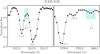 |
Fig. 4 Comparison of two Ir I lines in the spectrum of J1432–4125. The black dots represent the observed spectrum, and the turquoise boxes identify the position of the two lines. |
5.5 Dynamical origins and orbital properties
To investigate the possible origins of our stars, we explored their orbital properties in the E–Lz space. The total orbital energy (E) and the vertical component of the angular momentum (Lz) were derived from the phase-space coordinates of the stars using the galpy package (Bovy 2015), and their values are reported in Table 4. The results are visualized in the left panel of Fig. 5. This diagram displays the distribution of our sample stars in the orbital energy–angular momentum plane, where E is expressed in units of 105 km2 s−2 and Lz in 103 km s−1 kpc. The grayscale background represents the distribution of GALAH (GALactic Archaeology with HERMES) DR3 stars (Buder et al. 2021) within the metallicity range −1.3 ≤ [Fe/H] ≤ −0.9 dex. The thick black curve marks the dynamical boundary between in situ stars (with higher binding energies) and accreted populations (less bound) originally calculated in Belokurov & Kravtsov (2023) and shifted to the energy scale of the McMillan17 potential in Monty et al. (2024). The gray contours outline the region associated with the Gaia-Sausage-Enceladus (GSE) debris, as described by Belokurov & Kravtsov (2023) and adapted to our Galactic potential. In this space, two stars in our sample, J0040+2729 and J0217–1903, appear to lie within the GSE-defined region. To further test this hypothesis, we determined approximations for the orbital actions using the Stäckel fudge implemented in galpy (Mackereth & Bovy 2018) to create the so-called action diamond (Vasiliev 2019; Myeong et al. 2019), shown in the right panel of Fig. 5. This diagram plots the normalized azimuthal action, Jϕ/Jtot, against the vertical-minus-radial action, (Jz − JR)/Jtot, providing a compact view of the orbital morphology. Our ten stars are shown as colored markers, with the color indicating their orbital eccentricity, obtained by computing the orbital integrations over 3 Gyr with 1000 time steps per gigayear, assuming the McMillan17 Galactic potential (McMillan 2017) and Local Standard of Rest as Monty et al. (2024). The background grayscale again shows the distribution of GALAH stars, while the gray box marks the highest density region of GSE members in E–Lz space, according to Myeong et al. (2019).
Interestingly, while J0040+2729 and J0217–1903 appear within the GSE region in the E–Lz plane, they sit at the edge of the typical boundary in Jϕ/Jtot assumed for GSE members and well outside of the highest density region. This discrepancy indicates that their orbital morphologies are inconsistent with those of the GSE population, thereby weakening the case for their association with this major accretion event. Further support for this interpretation comes from their low metallicities of −2.72 and −2.86 dex, which are significantly below the characteristic GSE metallicity distribution, typically peaking around [Fe/H] ~ −1.5 (Myeong et al. 2019; Monty et al. 2020; Ceccarelli et al. 2024; Ou et al. 2024). Finally, the GSE is known to be depleted in [Eu/Fe] at low metallicities, with typical values of [Eu/Fe] being subsolar below [Fe/H] ~ −2.5 (Ou et al. 2024; Monty et al. 2024). These combined properties suggest that J0040+2729 and J0217–1903 may instead be associated with other halo substructures or represent remnants of distinct accretion events. The values of the actions and the eccentricity are reported in Table 4 (note that with an axisymmetric potential like (McMillan 2017), Jϕ = Lz).
In addition, we investigated whether any of the ten stars are associated with the chemodynamically tagged groups (CDTGs) identified by Gudin et al. (2021), Zepeda et al. (2023), and Shank et al. (2023). We find that only J0246–5124 belongs to one of the 36 CDTGs identified by Shank et al. (2023), while the remaining stars do not appear in any of the groups analyzed in these studies.
In summary, our dynamical analysis as mapped in Fig. 5, indicates that the ten stars in our sample likely originate from ten distinct astrophysical environments, each tracing separate r-process enrichment histories. Six of the stars (J0040+2729, J0217–1903, J0246–1518, J1430–2317, J1432–4125, and J2009–3410) lie above the dynamical boundary in the E–Lz plane (left panel of Fig. 5), consistent with an accreted origin, while three stars have prograde orbits and could have either formed in situ or been accreted, the last star have kinematics compatible with being a Milky Way disk star. Working from the hypothesis that nine of our stars are accreted from now-disrupted dwarf galaxies, and one star formed in the Milky Way we can use these stars to trace r-process enrichment over a wide range of environments and estimate an upper limit on the scatter between them.
Orbital angular momentum (Lz), actions (Jϕ, Jz, and Jr), orbital energy (E), and eccentricity (Ecc.) for the stars in our sample.
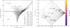 |
Fig. 5 Left panel: distribution of the sample stars in the orbital energy (E) versus angular momentum (Lz) plane. The grayscale background shows GALAH DR3 stars (Buder et al. 2021) with metallicities in the range −1.3 ≤ [Fe/H] ≤ −0.9. The thick black curve marks the boundary between dynamically in situ stars (more bound, lower energy) and accreted populations (less bound, higher energy), following the prescription of Monty et al. (2024). Colored markers indicate the 10 stars in our sample, as labeled in the legend. The gray contours identify the approximate region occupied by GSE stars from Belokurov & Kravtsov (2023), adapted to our adopted potential. Right panel: action-space diagram (“diamond diagram”) showing the normalized azimuthal action (Jϕ/Jtot) on the x-axis and the normalized vertical-minus-radial action ((Jz − JR)/Jtot) on the y-axis. Colored markers correspond to the same stars as in the left panel, now color-coded by their orbital eccentricity. The grayscale background shows again the GALAH DR3 comparison sample. The gray rectangular region marks the approximate locations of the Gaia-Sausage accreted substructure, following the definitions by Myeong et al. (2019). |
6 Discussion
This work presents one of the largest homogeneously and comprehensively analyzed samples of r-process-enhanced stars to date. While most previous studies have been limited to small samples, often focusing on one or two stars (Sneden et al. 2003; Christlieb et al. 2004; Aoki et al. 2010; Xylakis-Dornbusch et al. 2024), or relied on heterogeneous compilations from the literature, our study provides a systematic and self-consistent analysis of ten stars with robust abundance determinations. For each star, we derived abundances for over 50 species. Notably, this includes 29 neutron-capture elements, making our dataset uniquely suited to probe the detailed structure of the r-process abundance pattern. In addition, our kinematic analysis (Sect. 5.5) shows the stars are not linked to the same accreted structure, suggesting that they each trace an independent enrichment history. This provides a valuable opportunity to investigate the diversity of r-process nucleosynthesis pathways across distinct progenitor systems.
6.1 The r-process element abundance pattern
The complete r-process element abundance patterns for the ten stars in our sample are presented in Fig. 6, separated into light (30 ≤ Z < 55, left panel) and heavy (55 ≤ Z ≤ 92, right panel) r-process elements. The abundances for each star have been rescaled to the pattern of HD 222925 (gray dots and a solid line) by computing the average abundance offset with respect to this star (Roederer et al. 2018, 2022), separately for light and heavy elements. We use HD 222925 as a reference, as this exhibits the most comprehensive r-process pattern observed to date. For comparison, the Solar r-process pattern from Sneden et al. (2008) is shown as a dashed gray line. Residuals with respect to the average offset to HD 222925 for each star are shown in the lower panels. This rescaling approach allows us to assess the scatter in the r-process element abundance pattern, with minimal influence from scatter induced by the analysis, enabling a clearer comparison across stars. The resulting trends and deviations will be discussed in detail in the following subsections. Plots for the individual ten stars, each rescaled to the Eu values of HD 222925, are shown in Fig. C.1.
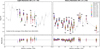 |
Fig. 6 Abundance patterns of light (30 ≤ Z < 55; left panel) and heavy neutron-capture elements (55 ≤ Z ≤ 92; right panel). The colored points represent derived abundances for the ten sample stars. The abundances for each star were rescaled by subtracting the mean offset from HD 222925 (Roederer et al. 2018). The pattern of HD 222925 is represented by the solid gray line and dots; upper limits are indicated with gray downward facing triangles. The lower panel displays the residuals with respect to the reference star HD 222925. The dashed gray line is the solar r-process pattern from Sneden et al. (2008). |
6.1.1 Light r-process elements
The production of the lightest neutron capture (n-capture) elements in the r-process has historically been seen to exhibit significant star-to-star variation when rescaled to Eu, leading to the view that their synthesis was not universal and potentially involved contributions from multiple astrophysical processes or sites (e.g., Travaglio et al. 2004; Hansen et al. 2012; Spite et al. 2018). This apparent lack of universality is contrasted with the relatively consistent patterns observed for the heavier lanthanides. However, recent work by Roederer et al. (2022) has challenged this picture by showing that several light trans-iron elements, including Se, Sr, Y, Nb, Mo, and Te, when scaled to Zr, follow a remarkably consistent abundance pattern in a sample of metal-poor, r-process-enriched stars with a dispersion ≤0.13 dex. These results suggest that, under certain astrophysical conditions, the production of light r-process elements may also reflect a universal mechanism, potentially tied to a common nucleosynthetic site.
This picture of universality among light r-process elements provides an important framework for interpreting our abundance measurements. In our sample, the Sr abundance presents a larger star-to-star variation compared to Y and Zr (see the left panel of Fig. 6), for which the universality seems to hold. However, Sr abundance was derived from the analysis of only three lines, compared to the other two elements for which over 20 clean transitions were investigated. The limited number of Sr lines and their characteristics (see Sect. 5.3.2) likely contribute to the larger observational spread.
The derived abundances of Mo, Ru, and Pd exhibit substantial star-to-star variation, as it is shown in Fig. 6. Such a spread is qualitatively consistent with the scenario proposed by Roederer et al. (2023), in which the deposition of fission fragments contributes to the element-to-element abundance scatter in metal-poor stars. However, the reliability of these measurements is affected by the fact that they are based on weak and often blended lines located in the near-UV region (3400–4000 Å). These observational challenges can introduce systematic uncertainties that may mimic or enhance real abundance variations. In particular, the Mo and Ru lines often lie in complex blended features, while the Pd lines are extremely weak and prone to contamination. As a result, it is difficult to determine whether the observed spread reflects true astrophysical scatter or is driven, at least in part, by measurement limitations. Alternative diagnostics would be necessary to disentangle observational effects from intrinsic abundance variations and to assess potential contributions from fission fragment yields in this mass region for this sample.
 |
Fig. 7 Cosmic standard deviation (σcosmic) of r-process element abundances across the stellar sample. Left: light r-process elements (normalized to Zr; shown as circles). Right: heavy r-process elements (normalized to Eu; shown as triangles). Only elements measured in at least three stars are included. Marker colors indicate the average number of spectral lines used for the abundance determination. The red horizontal line marks the standard deviation of [Zr/Eu], illustrating the overall variation between the light and heavy r-process components. |
6.1.2 Heavy r-process elements
The heaviest r-process elements, including the third r-process peak and the actinides, provide essential constraints on the astrophysical conditions and robustness of the r-process. Numerous studies have shown that, for a wide range of metal-poor stars enriched by the r-process, the abundance pattern of heavy elements from the second peak (Z ~ 56) to the third peak (Z ~ 76) closely follows the scaled solar r-process residuals (e.g., Westin et al. 2000; Sneden et al. 2008). This apparent invariance, often referred to as universality, suggests that a single type of r-process event (or at least a tightly constrained set of conditions) can robustly reproduce the heavy-element pattern over a wide range of progenitor environments. On the other end, the universality seems not to hold for the actinides, since some Milky Way halo stars show enhanced Th and U abundances relative to the rare earth elements (the so-called actinide boost; Hill et al. 2002; Holmbeck et al. 2018; Placco et al. 2023). The other extreme in the shape of actinide deficiency has also been detected in one star in the r-process-enhanced ultra-faint dwarf galaxy Reticulum II (Ji & Frebel 2018). Therefore, examining the abundances of Pb, Th, and U in our sample offers a valuable test of the robustness and possible diversity of the r-process at its heaviest end.
Across our sample, the abundances of elements from Ba to Er are consistently well determined and exhibit relatively small star-to-star scatter (see the right panel in Fig. 6). This behavior aligns with the previous findings, where elements beyond the second r-process peak are known to follow tight abundance trends, particularly in the highly r-process-enhanced stars. These elements are typically associated with strong, relatively unblended absorption lines in the optical range, which facilitates robust abundance determination, in particular in high-S/N spectra. However, in the same plot (Fig. 6), is shown how, at higher atomic numbers (Z ≥ 68), the observed scatter increases, likely due to a combination of weaker lines and more limited line availability.
Moving to the third peak, Os and Ir are strongly impacted by astrophysical and nuclear physics uncertainties, for example fission distributions, mass models, and beta decay rates (Arcones & Bertsch 2012; Vassh et al. 2020; Mumpower et al. 2024; Alencastro Puls et al. 2025). Despite their importance, Os and Ir abundances are notoriously difficult to derive in metal-poor stars due to the weakness of their lines, which are typically located in the crowded blue-UV region of the spectrum and often blended. For this reason, not many abundances of those elements were reported in literature before the recent work from Alencastro Puls et al. (2025) who published 33 Os I abundances plus five upper limit values and 32 Ir I plus eight upper limits. In our sample, Os and Ir show a larger dispersion, compared to the lanthanides, again likely due to the analysis of a single line as mentioned in Sect. 5.3.4.
Finally, the actinide element Th displays remarkable consistency across stars in our sample (Fig. 6), with no significant star-to-star dispersion, except for two clear outliers: J1430–2371 and J2009–3410. These two stars exhibit significantly lower Th abundances, with a rescaled log ϵ(Th/average of the offset from HD 222925) ratios of −0.30 and −0.37, respectively, compared to the average value of −0.05 of the other eight stars. This suggests a potential case of actinide depletion in these two stars, similar to what is observed in the Reticulum II star, contrasting with the otherwise uniform behavior of Th relative to Eu in the rest of the sample. However, we note that these two stars have the lowest effective temperatures in the sample. We therefore recommend caution in the interpretation of these abundances.
6.2 Cosmic abundance variations across independent r-process sites
As stated in Sect. 5.5, the ten stars analyzed in this study are chemically and dynamically untagged, and for the following further discussion, we therefore assume them to represent ten distinct r-process events. To provide a conservative upper limit, we assume that the measured abundance scatter for each element arises entirely from astrophysical origins, neglecting any contribution from observational uncertainties. We therefore refer to this scatter as “cosmic”, meaning that it is attributed entirely to astrophysical (rather than observational) causes. To quantify it, we computed the standard deviation of the abundance of each r-process element across the ten stars, after normalizing the light (Z < 55) and heavy (Z ≥ 55) elements to Zr and Eu, respectively, as shown in Fig. 7. The results for elements detected in at least three stars are shown in Fig. 5, where the standard deviations σ[X/Zr] and σ[X/Eu] are plotted as a function of atomic number, and color-coded by the average number of lines used for abundance determinations. We also plot the standard deviation of the σ[Zr/Eu] ratio itself, as a red horizontal line in the plot. This serves as a benchmark for the total variation between light and heavy r-process element production across the ten r-process events. The numerical values of the standard deviations of all the elements are reported in Table 5. For most elements, the spread is remarkably small: we find σ ≈ 0.04–0.09 dex (corresponding to fractional variations <18%) for the light r-process elements, and σ ≈ 0.08–0.12 dex (<24%) for the heavier elements. A few notable exceptions exist, including Ru, Tm, Yb, and Hf, where the dispersion exceeds σ[Zr/Eu]. However, the scatter observed for these elements among the ten stars is most likely driven by observational limitations rather than genuine astrophysical variations. For these elements, we inspected up to six spectral lines, but in most cases, only three or fewer could be reliably analyzed. This is considerably less than what is typically available for other lanthanides, as also illustrated in Table B.1. As a result, while the line-to-line scatter within individual stars remains small (as is clear from Table D.1), the abundance uncertainty, σ, in Table B.1 becomes larger whenever the determination relies on only a few lines. A similar situation applies to Lu, Os, and Ir: although their dispersions across the stars appear smaller, the robustness of their abundances is likewise limited by the very small number of available lines.
The larger variation in the σ[Zr/Eu] value is also expected, as this represents the scatter detected in numerous previous studies (see Sect. 6.1.1). This variation in the ratio of the light to heavy r-process elements can be directly compared to the lanthanide fraction of the r-process element production site. For example, the ejecta of the GW170817 kilonova event (Kasen et al. 2017) required a multicomponent model including lanthanide-poor and lanthanide-rich material to explain both the blue and red parts of the light curve. The lanthanide fraction for this event was later compared to r-process enriched stars by Ji et al. (2019), who found that this event did not produce enough lanthanide-rich material to match the stars. The σ[Zr/Eu] value of 0.18 dex found for our ten stars thus provides a range of lanthanide fractions. Since all ten stars in the sample presented here are r-process-enhanced (to varying degrees, as reflected by their [Eu/Fe] and [Ba/Eu] ratios) and did not originate from one common environment, we interpret the measured σcosmic values as the maximum allowed variation in abundance ratios produced by potentially up to ten independent r-process enrichment paths operating in the distinct environments where these stars formed.
This means that, regardless of the specific astrophysical origin, whether NSMs, magnetorotational supernovae, collapsars, magnetars, or other channels, any viable r-process site must reproduce element ratios consistent with the σcosmic constraints established here. In this sense, our measurements provide robust empirical bounds on the diversity of r-process nucleosynthesis pathways.
In order to investigate the potential effect of NLTE, we calculated the scatter among stars for which NLTE-corrected values for Sr, Ba, and Eu could be determined. The scatter with NLTE-corrected abundances are σ[Sr/Zr],NLTE = 0.11 and σBa/Eu,NLTE = 0.05. For comparison, the scatter in LTE abundances for the same six stars are σ[Sr/Zr],LTE = 0.06 and σ[Ba/Eu],LTE = 0.06. While the comparison is not fully straight-forward because only Sr was corrected in the [Sr/Zr] ratio, these results indicate that NLTE corrections tend to slightly reduce the scatter in [Ba/Eu] and increase it in [Sr/Zr], reflecting the differential impact of NLTE effects on different elements (see Table B.2).
Dispersion of light and heavy r-process element abundances among ten stars.
7 Summary
In this work, we present a homogeneous and comprehensive chemical abundance analysis of a sample of ten r-process-enhanced stars. These stars are characterized by strong enhancements in r-process elements and no significant s-process contribution, having a +0.39 ≤ [Eu/Fe] ≤ +1.06 and −1.01 ≤ [Ba/Fe] ≤ −0.52. For each star, we analyzed over 1400 spectral lines, deriving abundances for more than 50 species, including 29 neutron-capture elements from Rb to Th. The derived abundance patterns display the well-known universality for the heavy r-process elements (Ba to Ir), with only mild star-to-star variations. A slightly larger scatter is observed for Tm, Yb, and Hf, likely driven by increased measurement uncertainties due to line blending and continuum placement in the blue spectral region. A similar small scatter is seen for the light r-process elements in the range 38 ≤ Z ≤ 42, while the elements in the range 43 < Z ≲ 50 exhibit a somewhat larger dispersion across the sample, possibly in accordance with the fission fragment deposition scenario proposed by Roederer et al. (2023).
Kinematic analysis of the stars suggests they are not linked to a common birth environment but originated in distinct, unrelated progenitor systems. This sample thus offers valuable constraints on the diversity of ten individual astrophysical sites contributing to r-process enrichment. To quantify this, we calculated the cosmic standard deviation (σcosmic) for each element among the ten stars, representing ten different r-process nucleosynthesis sites. These values provide an upper limit to the possible variation introduced by different r-process nucleosynthesis environments across ten independent stellar sites and are remarkably small for the rare earth and third peak elements, for example σ[La/Eu] = 0.08 dex and σ[Os/Eu] = 0.11 dex. A somewhat larger scatter of 0.18 dex is seen between the light and heavy parts of the r-process pattern (σ[Zr/Eu]) representing the ratio between lanthanide-rich and lanthanide-poor ejecta for the ten enrichment paths.
Data availability
Atomic data tables and full Table B.1 are available at the CDS via https://cdsarc.cds.unistra.fr/viz-bin/cat/J/A+A/704/A282
Acknowledgements
The authors thank the referee for the insightful comments that helped improve the clarity of the paper. The authors also thank Alexander P. Ji for assistance with the observations. M.R. acknowledges support from the International Research Network for Nuclear Astrophysics (IReNA) through a Visiting Fellowship, which funded a research visit to North Carolina State University (U.S.) to collaborate with I.U.R. M.R. and T.T.H. acknowledge support from the Swedish Research Council (VR 2021-05556). I.U.R. acknowledges support from the US National Science Foundation (NSF) grant AST 2205847. A.F. acknowledges support from NSF-AAG grant AST-2307436. T.C.B. acknowledges partial support from grants PHY 14-30152; Physics Frontier Center/JINA Center for the Evolution of the Elements (JINA-CEE), and OISE-1927130; The International Research Network for Nuclear Astrophysics (IReNA), awarded by the US National Science Foundation, and DE-SC0023128CeNAM; the Center for Nuclear Astrophysics Across Messengers (CeNAM), awarded by the U.S. Department of Energy, Office of Science, Office of Nuclear Physics. E.M.H. acknowledges work performed under the auspices of the U.S. Department of Energy by Lawrence Livermore National Laboratory under Contract DE-AC52-07NA27344. This document has been approved for release under LLNL-JRNL-2008756. The work of V.M.P. is supported by NOIRLab, which is managed by the Association of Universities for Research in Astronomy (AURA) under a cooperative agreement with the U.S. National Science Foundation.
References
- Abbott, B. P., Abbott, R., Abbott, T. D., et al. 2017, APJ, 848, L13 [Google Scholar]
- Abbott, B. P., Abbott, R., Abbott, T. D., et al. 2019, APJ, 874, 163 [Google Scholar]
- Aldenius, M., Lundberg, H., & Blackwell-Whitehead, R. 2009, A&A, 502, 989 [NASA ADS] [CrossRef] [EDP Sciences] [Google Scholar]
- Alencastro Puls, A., Kuske, J., Hansen, C. J., et al. 2025, A&A, 693, A294 [NASA ADS] [CrossRef] [EDP Sciences] [Google Scholar]
- Amarsi, A. M., Asplund, M., Collet, R., & Leenaarts, J. 2015, MNRAS, 455, 3735 [Google Scholar]
- Amarsi, A. M., Barklem, P. S., Collet, R., Grevesse, N., & Asplund, M. 2019, A&A, 624, A111 [NASA ADS] [CrossRef] [EDP Sciences] [Google Scholar]
- Amarsi, A. M., Liljegren, S., & Nissen, P. E. 2022, A&A, 668, A68 [NASA ADS] [CrossRef] [EDP Sciences] [Google Scholar]
- Aoki, W., Beers, T. C., Christlieb, N., et al. 2007, ApJ, 655, 492 [NASA ADS] [CrossRef] [Google Scholar]
- Aoki, W., Beers, T. C., Honda, S., & Carollo, D. 2010, ApJ, 723, L201 [Google Scholar]
- Arcones, A., & Bertsch, G. F. 2012, Phys. Rev. Lett., 108, 151101 [Google Scholar]
- Arcones, A., & Thielemann, F.-K. 2012, J. Phys. G, 40, 013201 [Google Scholar]
- Asplund, M., Grevesse, N., Sauval, A. J., & Scott, P. 2009, ARA&A, 47, 481 [NASA ADS] [CrossRef] [Google Scholar]
- Bandyopadhyay, A., Ezzeddine, R., Allende Prieto, C., et al. 2024, ApJS, 274, 39 [Google Scholar]
- Barnes, J., & Metzger, B. D. 2022, APJ, 939, L29 [Google Scholar]
- Beers, T. C., & Christlieb, N. 2005, ARA&A, 43, 531 [NASA ADS] [CrossRef] [Google Scholar]
- Belmonte, M. T., Pickering, J. C., Ruffoni, M. P., et al. 2017, ApJ, 848, 125 [NASA ADS] [CrossRef] [Google Scholar]
- Belokurov, V., & Kravtsov, A. 2023, MNRAS, 525, 4456 [NASA ADS] [CrossRef] [Google Scholar]
- Bergemann, M. 2008, Phys. Scr. Vol. T, 133, 014013 [NASA ADS] [CrossRef] [Google Scholar]
- Bergemann, M. 2011, MNRAS, 413, 2184 [NASA ADS] [CrossRef] [Google Scholar]
- Bergemann, M., & Cescutti, G. 2010, A&A, 522, A9 [NASA ADS] [CrossRef] [EDP Sciences] [Google Scholar]
- Bergemann, M., & Gehren, T. 2008, A&A, 492, 823 [NASA ADS] [CrossRef] [EDP Sciences] [Google Scholar]
- Bernstein, R., Shectman, S. A., Gunnels, S. M., Mochnacki, S., & Athey, A. E. 2003, SPIE Conf. Ser., 4841, 1694 [NASA ADS] [Google Scholar]
- Biémont, É., Blagoev, K., Engström, L., et al. 2011, MNRAS, 414, 3350 [Google Scholar]
- Biémont, E., Garnir, H. P., Palmeri, P., Li, Z. S., & Svanberg, S. 2000, MNRAS, 312, 116 [CrossRef] [Google Scholar]
- Bovy, J. 2015, ApJS, 216, 29 [NASA ADS] [CrossRef] [Google Scholar]
- Buder, S., Sharma, S., Kos, J., et al. 2021, MNRAS, 506, 150 [NASA ADS] [CrossRef] [Google Scholar]
- Burbidge, E. M., Burbidge, G. R., Fowler, W. A., & Hoyle, F. 1957, RMP, 29, 547 [Google Scholar]
- Caliskan, S., Amarsi, A. M., Racca, M., et al. 2025, A&A, 696, A210 [NASA ADS] [CrossRef] [EDP Sciences] [Google Scholar]
- Cameron, A. G. W. 1957, AJ, 62, 9 [CrossRef] [Google Scholar]
- Canocchi, G., Morello, G., Lind, K., et al. 2024, A&A, 692, A43 [NASA ADS] [CrossRef] [EDP Sciences] [Google Scholar]
- Casey, A. R. 2014, PhD thesis, Australian National University, Canberra [Google Scholar]
- Castelli, F., & Kurucz, R. L. 2003, in Modelling of Stellar Atmospheres, 210, eds. N. Piskunov, W. W. Weiss, & D. F. Gray, A20 [Google Scholar]
- Ceccarelli, E., Massari, D., Mucciarelli, A., et al. 2024, A&A, 684, A37 [NASA ADS] [CrossRef] [EDP Sciences] [Google Scholar]
- Cescutti, G., Bonifacio, P., Caffau, E., et al. 2022, A&A, 668, A168 [NASA ADS] [CrossRef] [EDP Sciences] [Google Scholar]
- Chornock, R., Berger, E., Kasen, D., et al. 2017, APJ, 848, L19 [Google Scholar]
- Christlieb, N., Gustafsson, B., Korn, A. J., et al. 2004, ApJ, 603, 708 [NASA ADS] [CrossRef] [Google Scholar]
- Côté, B., Eichler, M., Arcones, A., et al. 2019a, ApJ, 875, 106 [Google Scholar]
- Cowan, J. J., Sneden, C., Beers, T. C., et al. 2005, ApJ, 627, 238 [NASA ADS] [CrossRef] [Google Scholar]
- Cowan, J. J., Sneden, C., Lawler, J. E., et al. 2021, RMP, 93, 015002 [CrossRef] [Google Scholar]
- Cutri, R. M., Skrutskie, M. F., van Dyk, S., et al. 2003, VizieR Online Data Catalog: 2MASS All-Sky Catalog of Point Sources (Cutri+ 2003), VizieR On-line Data Catalog: II/246. Originally published in: University of Massachusetts and Infrared Processing and Analysis Center, (IPAC/California Institute of Technology) (2003) [Google Scholar]
- Den Hartog, E. A., Lawler, J. E., Sneden, C., & Cowan, J. J. 2003, ApJS, 148, 543 [Google Scholar]
- Den Hartog, E. A., Lawler, J. E., Sneden, C., & Cowan, J. J. 2006, ApJS, 167, 292 [NASA ADS] [CrossRef] [Google Scholar]
- Den Hartog, E. A., Lawler, J. E., Sobeck, J. S., Sneden, C., & Cowan, J. J. 2011, ApJS, 194, 35 [NASA ADS] [CrossRef] [Google Scholar]
- Den Hartog, E. A., Ruffoni, M. P., Lawler, J. E., et al. 2014, ApJS, 215, 23 [NASA ADS] [CrossRef] [Google Scholar]
- Dixon, J. D., Ezzeddine, R., Li, Y., et al. 2025, ApJ, 994, 44 [Google Scholar]
- Drout, M. R., Piro, A. L., Shappee, B. J., et al. 2017, Science, 358, 1570 [NASA ADS] [CrossRef] [Google Scholar]
- Duquette, D. W., & Lawler, J. E. 1985, JOSA B, 2, 1948 [Google Scholar]
- Eichler, M., Arcones, A., Kelic, A., et al. 2015, APJ, 808, 30 [Google Scholar]
- Eitner, P., Bergemann, M., Ruiter, A. J., et al. 2023, A&A, 677, A151 [NASA ADS] [CrossRef] [EDP Sciences] [Google Scholar]
- Ezzeddine, R., Rasmussen, K., Frebel, A., et al. 2020, ApJ, 898, 150 [NASA ADS] [CrossRef] [Google Scholar]
- Fitzpatrick, M., Placco, V., Bolton, A., et al. 2024, arXiv e-prints [arXiv:2401.01982] [Google Scholar]
- Frebel, A., Casey, A. R., Jacobson, H. R., & Yu, Q. 2013, APJ, 769, 57 [Google Scholar]
- Gaia Collaboration (Babusiaux, C., et al.) 2018, A&A, 616, A10 [NASA ADS] [CrossRef] [EDP Sciences] [Google Scholar]
- Gaia Collaboration (Vallenari, A., et al.) 2023, A&A, 674, A1 [NASA ADS] [CrossRef] [EDP Sciences] [Google Scholar]
- Grichener, A., Kobayashi, C., & Soker, N. 2022, ApJ, 926, L9 [NASA ADS] [CrossRef] [Google Scholar]
- Gudin, D., Shank, D., Beers, T. C., et al. 2021, APJ, 908, 79 [Google Scholar]
- Halevi, G., & Mösta, P. 2018, MNRAS, 477, 2366 [NASA ADS] [CrossRef] [Google Scholar]
- Hansen, C. J., Primas, F., Hartman, H., et al. 2012, A&A, 545, A31 [NASA ADS] [CrossRef] [EDP Sciences] [Google Scholar]
- Hansen, T. T., Holmbeck, E. M., Beers, T. C., et al. 2018, APJ, 858, 92 [Google Scholar]
- Hill, V., Plez, B., Cayrel, R., et al. 2002, A&A, 387, 560 [CrossRef] [EDP Sciences] [Google Scholar]
- Holmbeck, E. M., & Andrews, J. J. 2024, APJ, 963, 110 [Google Scholar]
- Holmbeck, E. M., Beers, T. C., Roederer, I. U., et al. 2018, ApJ, 859, L24 [NASA ADS] [CrossRef] [Google Scholar]
- Holmbeck, E. M., Hansen, T. T., Beers, T. C., et al. 2020, ApJS, 249, 30 [NASA ADS] [CrossRef] [Google Scholar]
- Ivans, I. I., Simmerer, J., Sneden, C., et al. 2006, ApJ, 645, 613 [NASA ADS] [CrossRef] [Google Scholar]
- Ivarsson, S., Litzén, U., & Wahlgren, G. M. 2001, Phys. Scr, 64, 455 [CrossRef] [Google Scholar]
- Ji, A. P., & Frebel, A. 2018, ApJ, 856, 138 [NASA ADS] [CrossRef] [Google Scholar]
- Ji, A. P., Drout, M. R., & Hansen, T. T. 2019, APJ, 882, 40 [Google Scholar]
- Ji, A. P., Li, T. S., Simon, J. D., et al. 2020, ApJ, 889, 27 [NASA ADS] [CrossRef] [Google Scholar]
- Jin, S., & Soker, N. 2024, ApJ, 971, 189 [Google Scholar]
- Kasen, D., Metzger, B., Barnes, J., Quataert, E., & Ramirez-Ruiz, E. 2017, Nature, 551, 80 [Google Scholar]
- Kelson, D. D. 2003, PASP, 115, 688 [NASA ADS] [CrossRef] [Google Scholar]
- Kelson, D. D., Illingworth, G. D., van Dokkum, P. G., & Franx, M. 2000, ApJ, 531, 184 [NASA ADS] [CrossRef] [Google Scholar]
- Kramida, A., Ralchenko, Y., Nave, G., & Reader, J. 2018, in APS Meeting Abstracts, 2018, APS Division of Atomic, Molecular and Optical Physics Meeting Abstracts, M01.004 [Google Scholar]
- Kratz, K.-L., Farouqi, K., Pfeiffer, B., et al. 2007, APJ, 662, 39 [Google Scholar]
- Kurucz, R., & Bell, B. 1995, Atomic Line Data (R.L. Kurucz and B. Bell) Kurucz CD-ROM No. 23, Cambridge, 23 [Google Scholar]
- Kuske, J., Arcones, A., & Reichert, M. 2025, ApJ, 990, 37 [Google Scholar]
- Lagae, C., Amarsi, A. M., & Lind, K. 2025, A&A, 697, A60 [NASA ADS] [CrossRef] [EDP Sciences] [Google Scholar]
- Lattimer, J. M., & Schramm, D. N. 1974, ApJ, 192, L145 [NASA ADS] [CrossRef] [Google Scholar]
- Lawler, J. E., & Dakin, J. T. 1989, JOSA B, 6, 1457 [NASA ADS] [CrossRef] [Google Scholar]
- Lawler, J. E., Bonvallet, G., & Sneden, C. 2001a, ApJ, 556, 452 [NASA ADS] [CrossRef] [Google Scholar]
- Lawler, J. E., Wickliffe, M. E., Cowley, C. R., & Sneden, C. 2001b, ApJS, 137, 341 [NASA ADS] [CrossRef] [Google Scholar]
- Lawler, J. E., Wickliffe, M. E., den Hartog, E. A., & Sneden, C. 2001c, ApJ, 563, 1075 [CrossRef] [Google Scholar]
- Lawler, J. E., Wyart, J. F., & Blaise, J. 2001d, ApJS, 137, 351 [Google Scholar]
- Lawler, J. E., Sneden, C., & Cowan, J. J. 2004, ApJ, 604, 850 [Google Scholar]
- Lawler, J. E., Den Hartog, E. A., Sneden, C., & Cowan, J. J. 2006, ApJS, 162, 227 [Google Scholar]
- Lawler, J. E., den Hartog, E. A., Labby, Z. E., et al. 2007, ApJS, 169, 120 [Google Scholar]
- Lawler, J. E., Sneden, C., Cowan, J. J., et al. 2008, ApJS, 178, 71 [Google Scholar]
- Lawler, J. E., Sneden, C., Cowan, J. J., Ivans, I. I., & Den Hartog, E. A. 2009, ApJS, 182, 51 [Google Scholar]
- Lawler, J. E., Guzman, A., Wood, M. P., Sneden, C., & Cowan, J. J. 2013, ApJS, 205, 11 [Google Scholar]
- Lawler, J. E., Wood, M. P., Den Hartog, E. A., et al. 2014, ApJS, 215, 20 [CrossRef] [Google Scholar]
- Lawler, J. E., Sneden, C., & Cowan, J. J. 2015, ApJS, 220, 13 [NASA ADS] [CrossRef] [Google Scholar]
- Lawler, J. E., Sneden, C., Nave, G., et al. 2017, ApJS, 228, 10 [CrossRef] [Google Scholar]
- Li, R., Chatelain, R., Holt, R. A., et al. 2007, Phys. Scr, 76, 577 [NASA ADS] [CrossRef] [Google Scholar]
- Lind, K., & Amarsi, A. M. 2024, ARA&A, 62, 475 [NASA ADS] [CrossRef] [Google Scholar]
- Ljung, G., Nilsson, H., Asplund, M., & Johansson, S. 2006, A&A, 456, 1181 [NASA ADS] [CrossRef] [EDP Sciences] [Google Scholar]
- Mackereth, J. T., & Bovy, J. 2018, PASP, 130, 114501 [Google Scholar]
- Mashonkina, L. I., & Belyaev, A. K. 2019, Astron. Lett, 45, 341 [Google Scholar]
- Mashonkina, L., & Gehren, T. 2000, A&A, 364, 249 [NASA ADS] [Google Scholar]
- Mashonkina, L., Pakhomov, Y. V., Sitnova, T., et al. 2022, MNRAS, 509, 3626 [Google Scholar]
- Matsuno, T., Amarsi, A. M., Carlos, M., & Nissen, P. E. 2024, VizieR Online Data Catalog: 3D non-LTE Mg abundance (Matsuno+, 2024), VizieR On-line Data Catalog: J/A+A/ 688/A72. Originally published in: 2024A&A...688A..72M [Google Scholar]
- McCall, M. L. 2004, AJ, 128, 2144 [Google Scholar]
- McMillan, P. J. 2017, MNRAS, 465, 76 [NASA ADS] [CrossRef] [Google Scholar]
- McWilliam, A. 1998, AJ, 115, 1640 [NASA ADS] [CrossRef] [Google Scholar]
- Molero, M., Magrini, L., Matteucci, F., et al. 2023, MNRAS, 523, 2974 [NASA ADS] [CrossRef] [Google Scholar]
- Monty, S., Venn, K. A., Lane, J. M. M., Lokhorst, D., & Yong, D. 2020, MNRAS, 497, 1236 [NASA ADS] [CrossRef] [Google Scholar]
- Monty, S., Belokurov, V., Sanders, J. L., et al. 2024, MNRAS, 533, 2420 [NASA ADS] [CrossRef] [Google Scholar]
- Morton, D. C. 2000, ApJS, 130, 403 [Google Scholar]
- Mucciarelli, A., Bellazzini, M., & Massari, D. 2021, A&A, 653, A90 [NASA ADS] [CrossRef] [EDP Sciences] [Google Scholar]
- Mumpower, M. R., Sprouse, T. M., Miller, J. M., et al. 2024, ApJ, 970, 173 [Google Scholar]
- Munari, U., Henden, A., Frigo, A., et al. 2014, AJ, 148, 81 [NASA ADS] [CrossRef] [Google Scholar]
- Myeong, G. C., Vasiliev, E., Iorio, G., Evans, N. W., & Belokurov, V. 2019, MNRAS, 488, 1235 [Google Scholar]
- Nilsson, H., & Ivarsson, S. 2008, A&A, 492, 609 [NASA ADS] [CrossRef] [EDP Sciences] [Google Scholar]
- Nilsson, H., Ivarsson, S., Johansson, S., & Lundberg, H. 2002a, A&A, 381, 1090 [NASA ADS] [CrossRef] [EDP Sciences] [Google Scholar]
- Nilsson, H., Zhang, Z. G., Lundberg, H., Johansson, S., & Nordström, B. 2002b, A&A, 382, 368 [NASA ADS] [CrossRef] [EDP Sciences] [Google Scholar]
- Nishimura, S., Kotake, K., Hashimoto, M.-a., et al. 2006, APJ, 642, 410 [Google Scholar]
- Nordlander, T., & Lind, K. 2017, A&A, 607, A75 [NASA ADS] [CrossRef] [EDP Sciences] [Google Scholar]
- O’Brian, T. R., Wickliffe, M. E., Lawler, J. E., Whaling, W., & Brault, J. W. 1991, JOSA B, 8, 1185 [NASA ADS] [CrossRef] [Google Scholar]
- Ou, X., Ji, A. P., Frebel, A., Naidu, R. P., & Limberg, G. 2024, ApJ, 974, 232 [NASA ADS] [CrossRef] [Google Scholar]
- Patel, A., Metzger, B. D., Cehula, J., et al. 2025, APJ, 984, L29 [Google Scholar]
- Pehlivan Rhodin, A., Hartman, H., Nilsson, H., & Jönsson, P. 2017, A&A, 598, A102 [NASA ADS] [CrossRef] [EDP Sciences] [Google Scholar]
- Placco, V. M., Almeida-Fernandes, F., Holmbeck, E. M., et al. 2023, ApJ, 959, 60 [NASA ADS] [CrossRef] [Google Scholar]
- Placco, V. M., Frebel, A., Beers, T. C., & Stancliffe, R. J. 2014, ApJ, 797, 21 [Google Scholar]
- Placco, V. M., Sneden, C., Roederer, I. U., et al. 2021, RNAAS, 5, 92 [NASA ADS] [Google Scholar]
- Pols, O. R., Izzard, R. G., Stancliffe, R. J., & Glebbeek, E. 2012, A&A, 547, A76 [NASA ADS] [CrossRef] [EDP Sciences] [Google Scholar]
- Prasanna, T., Coleman, M. S. B., & Thompson, T. A. 2024, ApJ, 973, 91 [Google Scholar]
- Quinet, P., Palmeri, P., Biémont, É., et al. 2006, A&A, 448, 1207 [NASA ADS] [CrossRef] [EDP Sciences] [Google Scholar]
- Rodríguez Díaz, Lagae, Cis, Amarsi, Anish M., et al. 2024, A&A, 688, A212 [NASA ADS] [CrossRef] [EDP Sciences] [Google Scholar]
- Roederer, I. U., & Lawler, J. E. 2012, ApJ, 750, 76 [NASA ADS] [CrossRef] [Google Scholar]
- Roederer, I. U., Lawler, J. E., Sneden, C., et al. 2008, ApJ, 675, 723 [Google Scholar]
- Roederer, I. U., Lawler, J. E., Sobeck, J. S., et al. 2012, ApJS, 203, 27 [NASA ADS] [CrossRef] [Google Scholar]
- Roederer, I. U., Preston, G. W., Thompson, I. B., et al. 2014, AJ, 147, 136 [Google Scholar]
- Roederer, I. U., Sakari, C. M., Placco, V. M., et al. 2018, ApJ, 865, 129 [NASA ADS] [CrossRef] [Google Scholar]
- Roederer, I. U., Cowan, J. J., Pignatari, M., et al. 2022, ApJ, 936, 84 [CrossRef] [Google Scholar]
- Roederer, I. U., Vassh, N., Holmbeck, E. M., et al. 2023, Science, 382, 1177 [CrossRef] [PubMed] [Google Scholar]
- Ruffoni, M. P., Den Hartog, E. A., Lawler, J. E., et al. 2014, MNRAS, 441, 3127 [NASA ADS] [CrossRef] [Google Scholar]
- Sakari, C. M., Placco, V. M., Farrell, E. M., et al. 2018, ApJ, 868, 110 [Google Scholar]
- Schlafly, E. F., & Finkbeiner, D. P. 2011, ApJ, 737, 103 [Google Scholar]
- Shah, S. P., Ezzeddine, R., Roederer, I. U., et al. 2024, MNRAS, 529, 1917 [NASA ADS] [CrossRef] [Google Scholar]
- Shank, D., Beers, T. C., Placco, V. M., et al. 2023, APJ, 943, 23 [Google Scholar]
- Siegel, D. M., Barnes, J., & Metzger, B. D. 2019, Nature, 569, 241 [Google Scholar]
- Sitnova, T. M., Yakovleva, S. A., Belyaev, A. K., & Mashonkina, L. I. 2022, MNRAS, 515, 1510 [NASA ADS] [CrossRef] [Google Scholar]
- Skúladóttir, Á., & Salvadori, S. 2020, A&A, 634, L2 [NASA ADS] [CrossRef] [EDP Sciences] [Google Scholar]
- Sneden, C. A. 1973, PhD thesis, University of Texas, Austin [Google Scholar]
- Sneden, C., Cowan, J. J., Lawler, J. E., et al. 2003, ApJ, 591, 936 [NASA ADS] [CrossRef] [Google Scholar]
- Sneden, C., Cowan, J. J., & Gallino, R. 2008, ARA&A, 46, 241 [Google Scholar]
- Sneden, C., Lawler, J. E., Cowan, J. J., Ivans, I. I., & Hartog, E. A. D. 2009, APJSS, 182, 80 [Google Scholar]
- Sobeck, J. S., Lawler, J. E., & Sneden, C. 2007, ApJ, 667, 1267 [NASA ADS] [CrossRef] [Google Scholar]
- Sobeck, J. S., Kraft, R. P., Sneden, C., et al. 2011, AJ, 141, 175 [NASA ADS] [CrossRef] [Google Scholar]
- Soker, N. 2025, OJAp, 8, 67 [Google Scholar]
- Spite, F., Spite, M., Barbuy, B., et al. 2018, A&A, 611, A30 [NASA ADS] [CrossRef] [EDP Sciences] [Google Scholar]
- Storm, N., & Bergemann, M. 2023, MNRAS, 525, 3718 [NASA ADS] [CrossRef] [Google Scholar]
- Suntzeff, N. B. 1995, PASP, 107, 990 [Google Scholar]
- Tody, D. 1986, SPIE Conf. Ser., 627, 733 [Google Scholar]
- Tody, D. 1993, in Astronomical Society of the Pacific Conference Series, 52, Astronomical Data Analysis Software and Systems II, eds. R. J. Hanisch, R. J. V. Brissenden, & J. Barnes, 173 [Google Scholar]
- Travaglio, C., Gallino, R., Arnone, E., et al. 2004, APJ, 601, 864 [Google Scholar]
- Tsujimoto, T., & Shigeyama, T. 2014, A&A, 565, L5 [NASA ADS] [CrossRef] [EDP Sciences] [Google Scholar]
- van de Voort, F., Pakmor, R., Grand, R. J. J., et al. 2020, MNRAS, 494, 4867 [NASA ADS] [CrossRef] [Google Scholar]
- van de Voort, F., Pakmor, R., Bieri, R., & Grand, R. J. J. 2022, MNRAS, 512, 5258 [NASA ADS] [CrossRef] [Google Scholar]
- Vanbeveren, D., & Mennekens, N. 2024, Bull. Soc. R. Sci. Liège, 93, 338 [Google Scholar]
- Vasiliev, E. 2019, MNRAS, 484, 2832 [Google Scholar]
- Vassh, N., Mumpower, M. R., McLaughlin, G. C., Sprouse, T. M., & Surman, R. 2020, ApJ, 896, 28 [CrossRef] [Google Scholar]
- Villar, V. A., Guillochon, J., Berger, E., et al. 2017, ApJ, 851, L21 [Google Scholar]
- Wang, T., & Burrows, A. 2023, ApJ, 954, 114 [NASA ADS] [CrossRef] [Google Scholar]
- Westin, J., Sneden, C., Gustafsson, B., & Cowan, J. J. 2000, ApJ, 530, 783 [NASA ADS] [CrossRef] [Google Scholar]
- Wickliffe, M. E., & Lawler, J. E. 1997, JOSA B, 14, 737 [Google Scholar]
- Wickliffe, M. E., Salih, S., & Lawler, J. E. 1994, J. Quant. Spec. Radiat. Transf., 51, 545 [NASA ADS] [CrossRef] [Google Scholar]
- Wickliffe, M. E., Lawler, J. E., & Nave, G. 2000, J. Quant. Spec. Radiat. Transf., 66, 363 [NASA ADS] [CrossRef] [Google Scholar]
- Winteler, C., Käppeli, R., Perego, A., et al. 2012, APJ, 750, L22 [Google Scholar]
- Wood, M. P., Lawler, J. E., Sneden, C., & Cowan, J. J. 2013, ApJS, 208, 27 [NASA ADS] [CrossRef] [Google Scholar]
- Wood, M. P., Lawler, J. E., Den Hartog, E. A., Sneden, C., & Cowan, J. J. 2014a, ApJS, 214, 18 [Google Scholar]
- Wood, M. P., Lawler, J. E., Sneden, C., & Cowan, J. J. 2014b, ApJS, 211, 20 [NASA ADS] [CrossRef] [Google Scholar]
- Xu, H. L., Svanberg, S., Quinet, P., Palmeri, P., & Biémont, É. 2007, J. Quant. Spec. Radiat. Transf., 104, 52 [Google Scholar]
- Xylakis-Dornbusch, T., Hansen, T. T., Beers, T. C., et al. 2024, A&A, 688, A123 [NASA ADS] [CrossRef] [EDP Sciences] [Google Scholar]
- Zepeda, J., Beers, T. C., Placco, V. M., et al. 2023, APJ, 947, 23 [Google Scholar]
NOIRLab IRAF is distributed by the Community Science and Data Center at NSF NOIRLab), which is managed by the Association of Universities for Research in Astronomy (AURA) under a cooperative agreement with the U.S. National Science Foundation.
Appendix A Stellar parameters
 |
Fig. A.1 Logarithmic abundances (log ϵ) of Fe I and Fe II lines used to determine the stellar parameters of the sample stars, shown as a function of excitation potential (left), reduced EW (center), and wavelength (right). |
Appendix B Chemical abundances
Derived elemental abundances for J0040+2729.
NLTE abundance corrections.
Appendix C The ten r-process patterns
 |
Fig. C.1 r-process patterns of the ten stars in the sample (colored markers), each rescaled to the log ϵ(Eu) value of HD 222925 (solid gray line). The dashed gray line shows the solar r-process pattern from Sneden et al. (2008). |
Appendix D Atomic data
EW, atomic species, excitation potential (EP), oscillator strength (loggf), reduced equivalent width (REW), abundances (log(ϵ)), and references for every line analyzed in J0040+2729.
All Tables
Orbital angular momentum (Lz), actions (Jϕ, Jz, and Jr), orbital energy (E), and eccentricity (Ecc.) for the stars in our sample.
EW, atomic species, excitation potential (EP), oscillator strength (loggf), reduced equivalent width (REW), abundances (log(ϵ)), and references for every line analyzed in J0040+2729.
All Figures
|
Fig. 1 [Eu/Fe] as a function of [Fe/H], with a color gradient representing [Ba/Eu] for the sample of ten stars. All stars lie well above the canonical [Eu/Fe] > +0.3 threshold typically adopted for r-process-enhanced stars, and their low [Ba/Eu] values further confirm that the enrichment is consistent with a pure r-process origin. Gray stars in the background are taken from Roederer et al. (2014). |
| In the text | |
|
Fig. 2 [X/Fe] abundances of the light elements for the ten sample stars, compared to stellar abundances from the Milky Way halo (gray dots; Roederer et al. 2014). |
| In the text | |
|
Fig. 3 Examples of spectral synthesis fits used to derive elemental abundances. The observed data (black squares) are shown along with the best-fit synthetic spectra (solid teal lines) and associated uncertainties (shaded regions). The dotted lines correspond to synthetic spectra with no contribution from the indicated element (i.e., log ϵ = −∞). |
| In the text | |
|
Fig. 4 Comparison of two Ir I lines in the spectrum of J1432–4125. The black dots represent the observed spectrum, and the turquoise boxes identify the position of the two lines. |
| In the text | |
|
Fig. 5 Left panel: distribution of the sample stars in the orbital energy (E) versus angular momentum (Lz) plane. The grayscale background shows GALAH DR3 stars (Buder et al. 2021) with metallicities in the range −1.3 ≤ [Fe/H] ≤ −0.9. The thick black curve marks the boundary between dynamically in situ stars (more bound, lower energy) and accreted populations (less bound, higher energy), following the prescription of Monty et al. (2024). Colored markers indicate the 10 stars in our sample, as labeled in the legend. The gray contours identify the approximate region occupied by GSE stars from Belokurov & Kravtsov (2023), adapted to our adopted potential. Right panel: action-space diagram (“diamond diagram”) showing the normalized azimuthal action (Jϕ/Jtot) on the x-axis and the normalized vertical-minus-radial action ((Jz − JR)/Jtot) on the y-axis. Colored markers correspond to the same stars as in the left panel, now color-coded by their orbital eccentricity. The grayscale background shows again the GALAH DR3 comparison sample. The gray rectangular region marks the approximate locations of the Gaia-Sausage accreted substructure, following the definitions by Myeong et al. (2019). |
| In the text | |
|
Fig. 6 Abundance patterns of light (30 ≤ Z < 55; left panel) and heavy neutron-capture elements (55 ≤ Z ≤ 92; right panel). The colored points represent derived abundances for the ten sample stars. The abundances for each star were rescaled by subtracting the mean offset from HD 222925 (Roederer et al. 2018). The pattern of HD 222925 is represented by the solid gray line and dots; upper limits are indicated with gray downward facing triangles. The lower panel displays the residuals with respect to the reference star HD 222925. The dashed gray line is the solar r-process pattern from Sneden et al. (2008). |
| In the text | |
|
Fig. 7 Cosmic standard deviation (σcosmic) of r-process element abundances across the stellar sample. Left: light r-process elements (normalized to Zr; shown as circles). Right: heavy r-process elements (normalized to Eu; shown as triangles). Only elements measured in at least three stars are included. Marker colors indicate the average number of spectral lines used for the abundance determination. The red horizontal line marks the standard deviation of [Zr/Eu], illustrating the overall variation between the light and heavy r-process components. |
| In the text | |
|
Fig. A.1 Logarithmic abundances (log ϵ) of Fe I and Fe II lines used to determine the stellar parameters of the sample stars, shown as a function of excitation potential (left), reduced EW (center), and wavelength (right). |
| In the text | |
|
Fig. C.1 r-process patterns of the ten stars in the sample (colored markers), each rescaled to the log ϵ(Eu) value of HD 222925 (solid gray line). The dashed gray line shows the solar r-process pattern from Sneden et al. (2008). |
| In the text | |
Current usage metrics show cumulative count of Article Views (full-text article views including HTML views, PDF and ePub downloads, according to the available data) and Abstracts Views on Vision4Press platform.
Data correspond to usage on the plateform after 2015. The current usage metrics is available 48-96 hours after online publication and is updated daily on week days.
Initial download of the metrics may take a while.