| Issue |
A&A
Volume 705, January 2026
|
|
|---|---|---|
| Article Number | A81 | |
| Number of page(s) | 11 | |
| Section | Extragalactic astronomy | |
| DOI | https://doi.org/10.1051/0004-6361/202451456 | |
| Published online | 06 January 2026 | |
Resolving the molecular gas emission of the z ∼ 2.5–2.8 starburst galaxies SPT 0125-47 and SPT 2134-50
1
Department of Space, Earth & Environment, Chalmers University of Technology, SE-412 96 Gothenburg, Sweden
2
Institute of Physics, Laboratory of Astrophysics, École Polytechnique Fédérale de Lausanne (EPFL), Observatoire de Sauverny, Versoix 1290, Switzerland
★ Corresponding author: This email address is being protected from spambots. You need JavaScript enabled to view it.
Received:
11
July
2024
Accepted:
13
November
2025
Abstract
Context. The comoving cosmic star formation rate density peaks at z ∼ 2–3, with dusty star-forming galaxies being significant contributors to this peak. These galaxies are characterized by their high star formation rates and substantial infrared (IR) luminosities. The formation mechanisms remain an open question for these galaxies, particularly with respect to how such intense levels of star formation are triggered and maintained.
Aims. We aim to resolve CO(3–2) emission toward two strongly lensed galaxies, SPT 0125-47 and SPT 2134-50, at z ∼ 2.5–2.8 to determine their morphology and physical properties.
Methods. We used high-resolution ALMA band 3 observations of CO(3–2) emission toward both sources to investigate their properties. We performed parametric and nonparametric lens modeling using the publicly available lens modeling software PYAUTOLENS. We divided the CO(3–2) emission line into two bins corresponding to the red and blue portions of the emission line and nonparametrically modeled the source plane emission for both bins.
Results. We found that both sources are well described by a single Sérsic profile in both the parametric and nonparametric models of the source plane emission, in contrast to what was previously found for SPT 0125-47. Parametric lens modeling studies of the red and blue bins have reported distinctive differential magnification across the line spectrum. We performed a basic analysis of the morphology and kinematics in the source plane using nonparametric lens modeling of the red and blue bins. We found tentative evidence of a velocity gradient across both sources and no evidence of any clumpy structure, companions, or ongoing mergers.
Conclusions. The previously calculated high star formation rates and low depletion times of both SPT 0125-47 and SPT 2134-50 suggest that these galaxies are undergoing a dramatic phase in their evolution. Given the lack of evidence of ongoing interactions or mergers in our source plane models, we suggest that the intense star formation was triggered by a recent interaction and/or merger. We also consider the possibility that these galaxies might be in the process of settling into disks.
Key words: galaxies: evolution / galaxies: high-redshift / galaxies: interactions / galaxies: ISM / galaxies: starburst
© The Authors 2026
 Open Access article, published by EDP Sciences, under the terms of the Creative Commons Attribution License (https://creativecommons.org/licenses/by/4.0), which permits unrestricted use, distribution, and reproduction in any medium, provided the original work is properly cited.
This article is published in open access under the Subscribe to Open model. This email address is being protected from spambots. You need JavaScript enabled to view it. to support open access publication.
1. Introduction
The comoving cosmic star formation rate density is known to peak between z ∼ 2–3 (Madau & Dickinson 2014). A primary contributor to this peak is dusty star forming galaxies (DSFGs; Smail et al. 1998; Blain et al. 2002; Casey et al. 2014)1. These galaxies, occurring at redshifts z > 2, typically do not appear in optical wavelengths due to the UV light from their intense starbursts being reprocessed by dust into infrared (IR) wavelengths (e.g., Smail et al. 1997; Hughes et al. 1998; Bertoldi et al. 2000). These galaxies are known to have prodigious star formation rates of ≥1000 M⊙ yr−1 and high IR luminosities of ∼1013 L⊙ (e.g., Barger et al. 2014; Swinbank et al. 2014; Simpson et al. 2014). They have also been found to have relatively large molecular gas masses of 1010–1011 M⊙ and, thus, low molecular gas depletion timescales of ≲1 Gyr (e.g., Bothwell et al. 2013; Aravena et al. 2016; Birkin et al. 2021). DSFGs are considered to be similar to local ultraluminous IR galaxies (ULIRGs; Sanders & Mirabel 1996). Both have properties in common, including high molecular gas masses and IR luminosities (e.g., Tacconi et al. 2008; Engel et al. 2010; Riechers et al. 2011; Bothwell et al. 2013). Given these properties, it has been suggested that these galaxies will evolve into massive early-type galaxies (e.g., Simpson et al. 2014; Birkin et al. 2021).
One primary open question is how these galaxies obtain the fuel to maintain such intense star formation rates (SFRs). One explanation for this is based on the occurrence of mergers. Indeed, DSFGs have been shown to represent overdensities and, in some cases, show clear signs of mergers or interactions (e.g., Brodwin et al. 2008; Viero et al. 2009; Daddi et al. 2009; Capak et al. 2011; Kade et al. 2023). This is also consistent with simulations of massive galaxy evolution which have indicated the importance of mergers at high-redshift (e.g., Hopkins et al. 2008). Other studies have shown DSFGs can be single disk-like galaxies (e.g., Hodge et al. 2019; Rizzo et al. 2021; Amvrosiadis et al. 2025). Alternatively, the high SFRs observed in these galaxies may result from intensely star-forming clumps. Studies searched for these clumps in IR wavelengths with mixed results (e.g., Swinbank et al. 2010, 2015; Iono et al. 2016; Oteo et al. 2017). Hodge et al. (2016) found no evidence of clumps in dust continuum emission of 16 DSFGs, while Spilker et al. (2022) found clear evidence of clump-like structures in the z = 6.9 DSFG SPT 0311-58. Simulations suggest these clumps may occur on scales of 200–500 pc (e.g., Dekel et al. 2009; Bournaud et al. 2014), in good agreement with studies that detect these clumps. Observations of these clumps in high-redshift galaxies can provide additional constraints on mechanisms for star formation and the relation between stability and turbulence (Romeo et al. 2010; Romeo & Agertz 2014). However, the angular resolution necessary to resolve these scales is observationally challenging and expensive.
One method to improve the angular resolution of observations is to observe gravitationally lensed galaxies. In galaxy-galaxy lensing scenarios, this phenomenon can effectively improve the angular resolution of the observations by  , assuming a constant magnification factor across the image. Thus, high angular resolution observations from, for example, the Atacama Large Millimeter/Submillimeter Array (ALMA) can resolve down to the scales necessary to determine the morphology of DSFGs and determine whether they are composed of clumps or interacting galaxies. Studies investigating the properties of lensed DSFGs have become an increasingly common method for investigating the nature of these galaxies (e.g., Spilker et al. 2022; Amvrosiadis et al. 2025).
Indeed, studies often use observations of higher-J carbon monoxide (CO) transitions or brighter far-IR (FIR) emission lines such as [C II] fine structure emission line. However, lower-J CO transitions trace more diffuse molecular gas and are therefore key to determining the stability of clumps and disks. Cañameras et al. (2017) used CO(4–3) emission to study the strongly lensed z = 3.0 starburst galaxy, PLCK G244.8+54.9, with a source plane resolution of down to 60 pc. The authors found that at the given resolution, they were able to both observe clumpy structure and perform an investigation into the stability of the disk, finding that the disk was, in fact, stable while still hosting a massive starburst (Cañameras et al. 2017). In general, however, observations of lower-J CO transitions are seldom performed due to their observationally costly nature.
This paper studies the two strongly lensed DSFGs SPT 0125-47 and SPT 2134-50, originally discovered as bright sources in South Pole Telescope (SPT) data. These sources were originally selected to have S1.4 mm > 20 mJy, exhibit a dusty spectrum, and have no bright radio or far-IR (FIR) counterparts in the SPT data (Weiß et al. 2013). The original redshift detections for these sources come from a blind survey of CO(3–2) emission from Weiß et al. (2013). In addition, dust continuum emission has been observed in these galaxies in a variety of different wavelengths (Weiß et al. 2013; Spilker et al. 2016; Reuter et al. 2020). Aravena et al. (2016) used observations of CO(1–0) emission to determine the total molecular gas masses of both objects. Previous studies of these two sources used data with limited angular resolution and focused primarily on parametric lens mass modeling. Here we use data from a study designed to observe CO(3–2) in a selection of strongly gravitationally lensed galaxies. The original goal was to resolve down to scales of a few hundred parsecs in the source plane to compare any giant molecular clouds (GMCs) detected with local galaxy molecular gas scaling relations. We used these high-resolution observations to improve previous lens models, perform nonparametric modeling of the source plane emission, and, thus, the study the source-plane morphology of SPT 0125-47 and SPT 2134-50, specifically focusing on using nonparametric source plane lens modeling.
In Section 2, we describe the observations and data reduction steps. We present the results of the continuum, line analysis, and lens modeling in Section 3. We provide a discussion of our results in Section 4. Our conclusions are presented in Section 5. Throughout this paper, we adopt a flat Λ cold dark matter (ΛCDM) cosmology with H0 = 70 km s−1 Mpc−1 and Ωm = 0.3.
2. Observations and data reduction
SPT-S J012506-4723.7 (hereafter, SPT 0125-47) and SPT-S J213403-5013.4 (hereafter SPT 2134-50) were observed in band 3 as part of ALMA project ID 2016.1.01231.S (P.I. G. Drouart). The calibration and image processing steps were all performed in the Common Astronomy Software Application package (CASA; McMullin et al. 2007). The data for both sources were processed with the ALMA calibration pipeline in CASA 4.7.2, which includes the calibration of the phase, bandpass, flux, and gain. For SPT 0125-47, J2357-5311 was used as the bandpass and flux calibrator, J0124-5113 was used as the phase calibrator, and J0133-4430 was used as the check source. For SPT 2134-50, J2056-4714 was used as the bandpass and flux calibrator, J2124-4948 was used as the phase calibrator, and J2135-5006 was used as the check source. The pipeline-reduced data and diagnostic plots were visually inspected to ensure data quality, and additional flagging was added where necessary to ensure the calibration was satisfactory. The pipeline-reduced measurement sets were used to create images using the CASA task TCLEAN with a Hogbom deconvolution using private scripts in CASA version 5.6.2-3, where cleaning was performed in the region of expected emission. These images were used to identify line-free channels for continuum subtraction. The continuum was subtracted using the CASA task UVCONTSUB with a polynomial fit of order 1 for both SPT 0125-47 and SPT 2134-50. A natural weighting scheme was used when imaging the dust continuum emission. Emission line cubes were cleaned down to 1σ levels using TCLEAN and imaged using a natural weighting scheme with a spectral resolution of ∼70 km s−1, where 1σ = 0.5 mJy for SPT 0125-47 and 1σ = 0.36 mJy for SPT 2134-50. The residual images were checked for emission to ensure that the cleaning was adequate. The maximum recoverable scale was ≈15.2″ for SPT 0125-47 and ≈16.3″ for SPT 2134-50. We conservatively report the uncertainty in the absolute flux calibration to be ∼10% (note that the fiducial value in band 3 is 5%)2. Observational details for both sources are provide in Table 1.
Details of the observations.
3. Results
3.1. Continuum emission
We extracted the dust continuum emission for both sources from emission regions above 3σ within a chosen circular annular aperture shown in Fig. 1. We note that for both sources the continuum flux density is lower than the CO(3–2) emission. This is expected as the observations used in this work probe the longer wavelength regime and thereby the colder dust. We detect dust continuum emission toward SPT 0125-47 at 1.9 ± 1.4 mJy (not corrected for lensing) and toward SPT 2134-50 at 1.1 ± 0.7 mJy (not corrected for lensing). Both values are in good agreement with the value reported in Weiß et al. (2013)3. We show the continuum images for both SPT 0125-47 and SPT 2134-50 in Fig. 1.
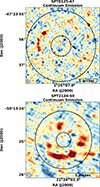 |
Fig. 1. Continuum image of SPT 0125-47 (top) and SPT 2134-50 (bottom). The contours are shown at −3, −2, 3, 4, 5σ levels. The synthesized beam is shown in the bottom left of each image. The black annulus shows the regions used to extract the dust continuum emission. |
3.2. Line emission
We detect CO(3–2) (rest frequency 345.7959899 GHz) emission toward both SPT 0125-47 and SPT 2134-50. We performed a regional extraction using a circular annular region (the same as that used for the continuum) of both spectra without including a σ cut to the data. The region of extraction is shown in Fig. 2. This methodology preserves fainter flux at emission edges, flux that a 5σ cut would exclude, making it particularly useful for analyzing “clumpy” structures. This approach was advantageous given the high angular resolution of the observations for both sources. To calculate the root mean square (rms) in each channel of the spectrum, we employed a straightforward sampling method. This involved sampling multiple emission-free regions of the cube in each channel, with the sampled regions matching the size of those used for spectrum extraction. The spectra of both sources are shown in Fig. 3. Due to the skewed profile of both emission line profiles, we fit the CO(3–2) emission with two Gaussian profiles (a single Gaussian does not provide a good fit to the data). We created moment-0 and moment-1 maps across the emission line, shown in Fig. 2. Line properties are provided in Table 2. Integrated flux densities and line luminosities were calculated using the following equations from Solomon et al. (1997):
![Mathematical equation: $$ \begin{aligned} L_{\rm line} = (1.04 \times 10^{-3})\,I_{\rm obs}\, \nu _{\rm rest}\,D^{2}_{L}\,(1+\textit{z})^{-1} [L_{\odot }], \end{aligned} $$](/articles/aa/full_html/2026/01/aa51456-24/aa51456-24-eq2.gif) (1)
(1)
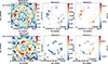 |
Fig. 2. Moment-0 and moment-1 maps of the CO(3–2) emission for SPT 0125-47 (top) and SPT 2134-50 (bottom). The first column shows the unmasked moment-0 map, the second column shows the moment-0 map masked to show only values above 3σ, and the third column shows the moment-1 map. The contours in the first two columns are shown at −3, −2, 3, 4, 5, 6, 7, 8, 9, 10σ levels. The synthesized beam is shown in the bottom left of each image. The black annulus in the unmasked moment-0 map for each source shows where the spectrum was extracted from. |
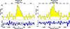 |
Fig. 3. Spectra of the CO(3–2) toward SPT 0125-47 (left) and SPT 2134-50 (right). In both cases, the spectrum is shown in the top panel, and the residuals from the Gaussian fit are shown in the bottom panel. The dashed blue line shows the two Gaussian fit to the spectra. The dashed gray line in the top panel and the shaded gray region in the lower panel indicate the per-channel RMS. Additionally, the top axis in the top panel of each spectrum displays the corresponding frequency. |
Line properties from our observations.
where Lline [L⊙] is the luminosity of the emission line, Iobs is the velocity integrated flux density (Iobs = SlineΔV [Jy km s−1]), Sline [mJy] is the observed flux density, and ΔV [km s−1] is the full width at half maximum (FWHM) of the emission line, νrest [GHz] is the rest-frame frequency of the line, DL [Mpc] is the luminosity distance and z is the redshift. This is expressed as
![Mathematical equation: $$ \begin{aligned} L^{\prime }_{\rm line} = (3.25 \times 10^7)\,I_{\rm obs}\,D^{2}_{L}\,(1+\textit{z})^{-3}\, \nu _{\rm obs}^{-2}\,[\mathrm{K}\,\mathrm{km}\,\mathrm{s}^{-1}\,\mathrm{pc}^{-2}], \end{aligned} $$](/articles/aa/full_html/2026/01/aa51456-24/aa51456-24-eq7.gif) (2)
(2)
where  is the luminosity of the emission line, Iobs is the velocity integrated flux density (Iobs = SlineΔV [Jy km s−1]), DL [Mpc] is the luminosity distance of the source, νrest [GHz] is the rest-frame frequency of the line, and z is the redshift.
3.3. Lens modeling
The lens modeling for both sources was performed using the sophisticated publicly available lens modeling code PYAUTOLENS (Nightingale et al. 2021). PYAUTOLENS has the ability to perform the lens modeling in the uv-plane and therefore on the interferometric visibilities rather than modeling the cleaned images. This is necessary for interferometric data as pixels in interferometric images are not independent of one another; therefore, performing lens modeling directly on the images can bias the results of the lens model. In this work, we performed all lens modeling on the UVCONTSUB measurement sets from CASA. PYAUTOLENS additionally has the capability of nonparametrically modeling the source emission, which bypasses the need to assume a specific source-plane morphology (e.g., Sérsic light profiles). We used PYAUTOLENS to perform both parametric and nonparametric modeling of the CO(3–2) emission toward both sources wherein only the channels containing line emission were used in the modeling. We first performed parametric lensing to optimize the lens mass model then perform nonparametric lens modeling using this mass model. We attempted to model the dust continuum emission using both parametric and nonparametric source plane models, but found that the signal-to-noise (S/N) of the data was too poor to obtain reasonable results. We therefore limited the modeling to the CO(3–2) emission.
3.3.1. Parametric source modeling
We first performed parametric modeling to establish a working lens model. This is often done on continuum emission as it can be stronger than the corresponding line emission. This method has been used previously for both SPT 0125-47 and SPT 2134-50 (Spilker et al. 2016). Here, we performed lens modeling directly on the CO(3–2) emission and subsequently applied the best-fit lens model to the continuum data due to the continuum data having significantly lower S/N than the CO(3–2) emission.
Both sources are in galaxy-galaxy lensing morphologies. For both sources we model the lens as a single isothermal ellipsoid (SIE) mass distribution assumed to not have light distributions in the frequencies covered by the ALMA observations. These lens mass distributions were parameterized by their (x, y) offset from the observational phase center, Einstein radius, axis ratio, and position angle. We fixed the centers of the mass distributions to be in the center of the observed Einstein rings using uniform priors. We set an upper limit on the Einstein radius for both sources as slightly larger than the Einstein radius reported for the sources in Spilker et al. (2016). All other parameters were free.
The sources were parameterized as Sérsic light distributions using linear light profiles. Linear light profiles minimize the degeneracy between the effective radius and the intensity of the source by solving for both of these parameters using linear algebra. The sources were parameterized by their (x, y) offset from the observational phase center, axis ratio, position angle, effective radius, and Sérsic index. We provide best-fit source and lens parameters in Table A.1 and Table A.2. We show the images, models, and residuals for both SPT 0125-47 and SPT 2134-50 in Fig. 4.
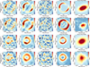 |
Fig. 4. Parametric (rows 1 and 3) and pixelized (rows 2 and 4) lens modeling of the CO(3–2) emission detected in SPT 0125-47 (top two rows) and SPT 2134-50 (bottom two rows). The first column displays the dirty image generated by PYAUTOLENS, with contours at −3, 3, 4, 5, 6, 7, 8, 9, 10σ levels. Note: this is not a cleaned image, so structures may differ slightly from those in cleaned images. The second column presents the dirty model image from PYAUTOLENS, also with contours at −3, 3, 4, 5, 6, 7, 8, 9, 10σ levels. The third column shows the dirty residual image produced by PYAUTOLENS, with contours at −3, 3, 4, 5σ levels. The fourth column illustrates the image plane emission parametric/pixelized model of the data, produced by PYAUTOLENS, with the black line representing the critical line. The fifth column shows the source plane emission parametric+pixelized model of the data from PYAUTOLENS, with the black line indicating the caustic line. All images are centered around the ALMA phase center. |
We note that the primary interest of this paper is the results of nonparametric lens modeling and, therefore, the parametric lens modeling was only performed to: (i) optimize the lens mass model, which was then used for the nonparametric fitting; (ii) obtain lens magnification factors, and (iii) compare our results with literature values.
3.3.2. Nonparametric source modeling
After establishing an optimized lens model from the parametric lens modeling, we used this lens model to nonparametrically model the source emission. This methodology employs an adaptive Voronoi mesh, maintaining regions of higher magnification and, thus, higher angular resolution, around the caustic lines in the source plane. PYAUTOLENS uses a regularization scheme when performing the nonparametric modeling to maintain a balance between over-smoothing and over-fitting the source plane emission (Nightingale et al. 2021). Here, we used a constant regularization scheme, which was parameterized by a regularization coefficient that regulated the smoothness of the emission. The images are then interpolated to a square grid for easier analysis. We used a similar methodology to what has been employed for other studies that perform nonparametric lensing using PYAUTOLENS (e.g., Maresca et al. 2022; Giulietti et al. 2023; Perrotta et al. 2023; Amvrosiadis et al. 2025). We show the images, models, and residuals for both the nonparametric models of the CO(3–2) for both SPT 0125-47 and SPT 2134-50 in Fig. 4.
We note that the errors reported in Tables A.1 and A.2 are formal statistical errors from the sampling algorithms in the lens model fitting. This does not provide a good estimation of the systemic errors, in particular, those associated with the nonparametric lensing. We created source plane error maps with PYAUTOLENS using the same procedure described above, but using the visibility errors, extracted using CASA’s STATWT task, instead of the CO(3–2) emission. These error maps show the rms in each Voronoi cell, interpolated onto a square grid. The maps demonstrate how errors propagate from the image plane to the source plane, making it straightforward to produce a S/N map in the source plane. We show the intensity maps, error maps, and S/N maps in Fig. 5. The error map has been normalized by the maximum of the intensity map and it can therefore be interpreted as a per-pixel percentage error.
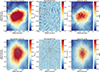 |
Fig. 5. Source plane intensity (left), intensity error maps (middle), and S/N maps (i.e., intensity divided by intensity error, right) for SPT 0125-47 and SPT 2134-50. The gray polygons show the Voronoi mesh used for the pixelized reconstruction and the black line shows the caustic line. Both the intensity and intensity error maps are normalized, where the error maps have been normalized to the maximum of the intensity map, meaning that the value can be seen as a percentage error per pixel. The S/N map provides a measure of the significance of the reconstructed emission. |
3.3.3. SPT 0125-47
We found a good parametric lens mass model for the CO(3–2) emission with no residuals at > 3σ levels. Parametric modeling of this source required using a single-lens mass distribution and, similarly, a single Sérsic source profile, unlike the three sources required in Spilker et al. (2016). Through this methodology we found a magnification factor of μCO(3 − 2) = 10.7 ± 0.002. This value is lower than what was found for CO(1–0) emission in Aravena et al. (2016); however, we note that the cited study did not directly model the CO(1–0) emission; rather, these authors calculated the magnification factor from the width of the emission line. This methodology is not as robust as modeling the line emission and therefore we suggest that the magnification factor reported here is a more accurate representation of the magnification affecting the CO molecular gas in SPT 0125-47.
We used the optimized lens model from the CO(3–2) emission to create nonparametric models for the CO(3–2) emission. We find that both the parametric and nonparametric source plane models do not require the use of multiple source Sérsic profiles, as is the case in Spilker et al. (2016). We further discuss this in Section 4.2.
3.3.4. SPT 2134-50
We found a good parametric lens mass model for the CO(3–2) emission with limited residuals at ∼3σ levels, but we note that these residuals do not appear to be directly correlated with the Einstein ring of emission from SPT 2134-50 and might simply be due to noise. Through this methodology, we find a magnification factor of μCO(3 − 2) = 7.6 ± 0.002. This is very similar to the value reported in Aravena et al. (2016); however, similarly to the case of SPT 0125-47, we suggest that the methodology employed here is more robust; therefore, this value should be considered the accurate magnification value for the CO emission. As with SPT 0125-47, we used the optimized lens model from the CO(3–2) emission to nonparametrically model the CO(3–2) emission. We found a very similar source plane morphology between the parametric and nonparametric models for the CO(3–2).
4. Discussion
4.1. Differential lensing
The spectral line profiles of both SPT 0125-47 and SPT 2134-50 exhibit skewed profiles wherein red spectral regions appear weaker than blue spectral regions. We investigated whether this is caused by differential lensing across the line profile by dividing each emission line into red and blue spectral bins. We show these regions in relation to the entire spectrum for both sources in Fig. B.1. We then performed a parametric lens modeling on the red and blue regions of the spectrum for both sources using the best-fit lens model (the same procedure is described in Section 3.3).
Both sources showed significantly different magnification factors between the red and blue regions of the spectrum. For SPT 0125-47, we found μblue ∼ 14 and μred ∼ 9. For SPT 2134-50, we found μblue ∼ 14 and μred ∼ 4.4. Full per-channel spectral lensing correction (e.g., Kade et al. 2024a) is not feasible given the relatively low per-channel S/N of these observations (≲5σ per channel). Higher sensitivity data or observations of a brighter emission line could potentially allow for a full reconstruction. These red and blue models provide clear evidence that the skewed spectral profiles and, thus, the necessity of fitting with two Gaussian profiles, result, at least in part, from differential lensing. In this scenario, bluer regions of the spectrum experience higher magnification and therefore would be less bright in a per-channel magnification-corrected spectrum, resulting in a wider and flatter line profile. We note that this could also result in a profile resembling a double-horned profile, which could be associated with rotation; we provide a short discussion on this in Section 4.2. We caution that future studies of these two sources should consider the possible effect of differential lensing on, for instance, kinematical modeling.
4.2. Source plane properties
Recent studies have demonstrated the importance of nonparametric, pixelized, source plane models of lensed galaxies to accurately interpret lensed source properties including kinematics and morphology (e.g., Rybak et al. 2020; Rizzo et al. 2021; Giulietti et al. 2023; Perrotta et al. 2023; Amvrosiadis et al. 2025). Although the approximate morphology of the parametric and nonparametric modeling are consistent with each other with regard to the location of the background source (e.g., in relation to the caustic line), the main discrepancy lies in the lack of detail in the parametric models. This highlights the importance of modeling that avoids making a priori assumptions about the source plane morphology. We discuss the morphology and kinematics of the two sources in the pixelized source plane models below.
4.2.1. Morphology
SPT 0125-47 was previously reported as a system composed of three different galaxies with one member dominating in brightness (Spilker et al. 2016). This conclusion was based on parametric lens modeling of the morphology of the 870 μm dust continuum emission. In this study, we found that our parametric lens model does not require multiple sources to obtain a good fit with no significant residual emission. We also found a similar source plane morphology in the nonparametric model.
SPT 2134-50 was previously reported as a single galaxy system (Spilker et al. 2016), which is in good agreement with the results of the parametric lens modeling in this work. In general, we found that both SPT 0125-47 and SPT 2134-50 have smooth source plane morphologies in the nonparametric models.
We performed a brief investigation into whether we should expect to be able to resolve clumps in source plane models based on the expected size of clumps found in previous studies. For SPT 0125-47, assuming a static magnification factor across the image, the source-plane beam is  , corresponding to ∼270 pc. This means that we can only clearly resolve features on scales larger than ∼800 pc. For SPT 2134-50, under the same assumption of the static source plane beam, the source-plane beam is
  , corresponding to ∼400 pc. This means that we can only clearly resolve features on scales larger than
  . Values for the expected size of clumps in the interstellar medium (ISM) as found by simulations and observations are significantly smaller than these scales (e.g., Dekel et al. 2009; Bournaud et al. 2014; Romeo & Agertz 2014; Iono et al. 2016; Oteo et al. 2017). For example, Spilker et al. (2022) studied the z = 6.9 DSFG SPT 0311-58 and found clumps on scales of a few hundred parsecs; in addition, we note that similar scales were found in Rybak et al. (2020). Therefore, even at the relatively high angular resolutions of the observations in this work, it is not possible to resolve features on the scale of the expected clump size, regardless of any of the lens modeling uncertainties or difficulties.
4.2.2. Kinematics
Studies such as Rizzo et al. (2021) and Amvrosiadis et al. (2025) have performed kinematical analyses on lensed galaxies, in particular, lensed SPT sources. This type of analysis requires the creation of a de-lensed source plane emission cube. The relatively low per-channel S/N of the CO(3–2) emission prevents the construction of a fully delensed source plane spectral cube. Source plane models based on the entire integrated emission line already exhibit substantial uncertainties. Only a few regions achieve high significance (S/N > 5), while most regions are at S/N ∼ 2–3 (see Fig. 5). We performed two initial attempts to construct a delensed source plane using a restricted number of channels centered on the brightest regions of the spectrum, selecting approximately ten channels per source. However, the S/N in the individual channels was insufficient to enable reliable source-plane modeling. A further attempt using only three channels also yielded unsuccessful results.
Instead, we used the red and blue spectral bins (Section 4.1) to create pixelized source-plane models for these bins for each source. While this approach yielded acceptable results, the S/N remains low with considerable source plane uncertainties. For example, in the case of SPT 2134-50, there are no regions of the image with S/N > 3 in the red bin. The channel maps and associated uncertainty and S/N maps are shown in Figs. 6 and 7. We found tentative evidence of a velocity gradient across both sources, which might be indicative of more ordered rotation in these sources, although the current data do not allow for the construction of reliable source-plane moment-1 maps, which would be required to further investigate this possibility. Given the quality of the reconstructions, we urge caution when drawing conclusions based on these source plane reconstructions. Deep, high-sensitivity observations of a bright emission line such as [C II] or higher-J CO lines, with comparable or higher angular resolution, would be necessary to confirm and characterize these possible velocity structures.
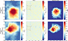 |
Fig. 6. Pixelized source plane models for the red and blue bins for SPT 0125-47, as described in Section 4.2.2 with source plane intensity (left), intensity error maps (middle), and S/N maps (i.e., intensity divided by intensity error, right). The gray polygons show the Voronoi mesh used for the pixelized reconstruction and the black line shows the caustic line. Both the intensity and intensity error maps are normalized, where the error maps have been normalized to the maximum of the intensity map, meaning that the value can be seen as a percentage error per pixel. |
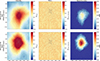 |
Fig. 7. Pixelized source plane models for the red and blue bins for SPT 2134-50 as described in Section 4.2.2 with source plane intensity (left), intensity error maps (middle), and S/N maps (i.e., intensity divided by intensity error: right). The gray polygons show the Voronoi mesh used for the pixelized reconstruction and the black line shows the caustic line. Both the intensity and intensity error maps are normalized, where the error maps have been normalized to the maximum of the intensity map, meaning that the value can be seen as a percentage error per pixel. |
4.2.3. Implications
We calculated the depletion time (tdep = SFR/Mgas) for both sources using the total molecular gas mass and IR luminosity from Aravena et al. (2016) and following the procedure within. This value is not dependent on the lensing magnification. We found a depletion time of 0.051 Gyr for SPT 0125-47 and 0.037 Gyr for SPT 2134-50. These values are in good agreement with the depletion times found for other SPT sources (Aravena et al. 2016). Both sources lie well below the expected depletion timescales for main sequence (MS) galaxies from Saintonge et al. (2013) as expected given their significantly elevated SFRs above MS galaxies. The high SFRs and short depletion times could be interpreted as an indication that both systems have recently experienced an interaction and/or merger, which could explain their high IR luminosities and how these sources had obtained sufficient gas to sustain such high SFRs.
This could represent a situation similar to the DSFG G09v1.97 at z = 3.63 (Kade et al. 2024b). This is an attractive explanation as it follows the classical picture of massive galaxy evolution (e.g., Hopkins et al. 2008), but it is only one of many possibilities which, given the current data quality, are infeasible to verify. For example, it is entirely conceivable that improved observations of a stronger emission line would show these sources breaking into multiple sources, possibly as part of the process of merging or simply by virtue of being spatially close to each other. An additional scenario is that these sources represent examples of more secular evolution, wherein cold mode accretion is the primary galaxy growth mechanism in operation (e.g., Kereš et al. 2005).
Our analysis demonstrates that high-S/N data are essential for reliable pixelized source plane reconstructions. Given the observational constraints of these data, these results should be considered as preliminary and require confirmation through deeper observations or observations of brighter emission lines (e.g., [C II]). Although pixelized reconstructions remain the optimal method for interpreting strongly gravitationally lensed galaxies, future benchmarking studies are necessary to establish the S/N requirements for robust kinematic analyses. However, such work falls outside the scope of this paper. These findings underscore the value of pixelized source plane reconstructions, and the caution necessary when interpreting results from this method, while highlighting the observational difficulties inherent to high-redshift ISM studies.
5. Conclusions
In this paper, we present the detection of high-resolution ALMA observations of CO(3–2) emission in two lensed sources, SPT 0125-47 and SPT 2134-50. We describe the parametric and nonparametric lens modeling we performed on both galaxies using PYAUTOLENS. Our conclusions are listed below.
-
We have further improved the lens models of SPT 0125-47 and SPT 2134-50 using the publicly available code PYAUTOLENS. We find that both sources require only a single Sérsic profile as a description of the background source to obtain a good lens model, in contrast to previous findings.
-
We found clear evidence of differential lensing across the spectrum for both SPT 0125-47 and SPT 2134-50. With the current data availability, a full per-channel magnification correction is not feasible. However, we emphasize that the effect is not insignificant and should be taken into account in future studies of these two sources.
-
We divided the line profile of both sources into two red and blue bins of the spectra and performed pixelized reconstructions of these bins. In the two-bin scenario, we found evidence of a velocity gradient, but given the very tentative nature of this detection, we did not investigate this possibility further.
-
We find that the parametric and pixelized models of both SPT 0125-47 and SPT 2134-50 suggest a single background source. However, we note that the source plane resolution is not sufficient to conclusively determine whether both of them are composed of multiple smaller galaxies in an ongoing merger or a single disk.
Given the very high SFRs and low depletion times found in previous studies and reported here, combined with the lack of evidence of interactions or mergers in our source plane emission models, we suggest that these sources have recently undergone an interaction or merger that triggered the high SFR. In such a case, these sources would both be in the process of settling into disks. Very-high-angular-resolution observations of a brighter emission line, such as [C II], combined with pixelized source plane modeling would be necessary to arrive at robust conclusions on the true nature of these two sources.
These galaxies are often also referred to as submillimeter galaxies (SMG). Historically, SMGs have been defined as being bright at submillimeter wavelengths, typically with 850 μm flux density S850 > 3 − 5 mJy. Both galaxies in this work would be SMGs in this classification methodology.
Given that these continuum measurements are in good agreement with previous measurements at the same wavelength, we do not pursue spectral energy distribution (SED) fitting.
Acknowledgments
We thank the anonymous referee for constructive feedback that helped improve the clarity of the manuscript. K.K. acknowledges support from the Nordic ALMA Regional Centre (ARC) node based at Onsala Space Observatory. The Nordic ARC node is funded through Swedish Research Council grant No. 2017-00648. K.Kn. acknowledges support from the Knut and Alice Wallenberg Foundation (KAW 2017.0292). S.K. gratefully acknowledges funding from the European Research Council (ERC) under the European Union’s Horizon 2020 research and innovation programme (grant agreement No. 789410). This paper makes use of the following ALMA data: ADS/JAO.ALMA#2016.1.01231.S. ALMA is a partnership of ESO (representing its member states), NSF (USA) and NINS (Japan), together with NRC (Canada), NSTC and ASIAA (Taiwan), and KASI (Republic of Korea), in cooperation with the Republic of Chile. The Joint ALMA Observatory is operated by ESO, AUI/NRAO and NAOJ.
References
- Amvrosiadis, A., Lange, S., Nightingale, J. W., et al. 2025, MNRAS, 537, 1163 [Google Scholar]
- Aravena, M., Spilker, J. S., Bethermin, M., et al. 2016, MNRAS, 457, 4406 [Google Scholar]
- Barger, A. J., Cowie, L. L., Chen, C. C., et al. 2014, ApJ, 784, 9 [NASA ADS] [CrossRef] [Google Scholar]
- Bertoldi, F., Carilli, C. L., Menten, K. M., et al. 2000, A&A, 360, 92 [Google Scholar]
- Birkin, J. E., Weiss, A., Wardlow, J. L., et al. 2021, MNRAS, 501, 3926 [Google Scholar]
- Blain, A. W., Smail, I., Ivison, R. J., Kneib, J. P., & Frayer, D. T. 2002, Phys. Rep., 369, 111 [Google Scholar]
- Bothwell, M. S., Maiolino, R., Kennicutt, R., et al. 2013, MNRAS, 433, 1425 [Google Scholar]
- Bournaud, F., Perret, V., Renaud, F., et al. 2014, ApJ, 780, 57 [Google Scholar]
- Brodwin, M., Dey, A., Brown, M. J. I., et al. 2008, ApJ, 687, L65 [Google Scholar]
- Cañameras, R., Nesvadba, N., Kneissl, R., et al. 2017, A&A, 604, A117 [Google Scholar]
- Capak, P. L., Riechers, D., Scoville, N. Z., et al. 2011, Nature, 470, 233 [Google Scholar]
- Casey, C. M., Narayanan, D., & Cooray, A. 2014, Phys. Rep., 541, 45 [Google Scholar]
- Daddi, E., Dannerbauer, H., Stern, D., et al. 2009, ApJ, 694, 1517 [Google Scholar]
- Dekel, A., Sari, R., & Ceverino, D. 2009, ApJ, 703, 785 [Google Scholar]
- Engel, H., Tacconi, L. J., Davies, R. I., et al. 2010, ApJ, 724, 233 [NASA ADS] [CrossRef] [Google Scholar]
- Giulietti, M., Lapi, A., Massardi, M., et al. 2023, ApJ, 943, 151 [NASA ADS] [CrossRef] [Google Scholar]
- Hodge, J. A., Swinbank, A. M., Simpson, J. M., et al. 2016, ApJ, 833, 103 [Google Scholar]
- Hodge, J. A., Smail, I., Walter, F., et al. 2019, ApJ, 876, 130 [Google Scholar]
- Hopkins, P. F., Hernquist, L., Cox, T. J., & Kereš, D. 2008, ApJS, 175, 356 [Google Scholar]
- Hughes, D. H., Dunlop, J. S., Archibald, E. N., Rawlings, S., & Eales, S. A. 1998, arXiv e-prints [arXiv:astro-ph/9810253] [Google Scholar]
- Iono, D., Yun, M. S., Aretxaga, I., et al. 2016, ApJ, 829, L10 [Google Scholar]
- Kade, K., Knudsen, K. K., Vlemmings, W., et al. 2023, A&A, 673, A116 [NASA ADS] [CrossRef] [EDP Sciences] [Google Scholar]
- Kade, K., Knudsen, K. K., Bewketu Belete, A., et al. 2024a, A&A, 684, A56 [NASA ADS] [CrossRef] [EDP Sciences] [Google Scholar]
- Kade, K., Yang, C., Yttergren, M., et al. 2024b, A&A, submitted [NASA ADS] [CrossRef] [EDP Sciences] [Google Scholar]
- Kereš, D., Katz, N., Weinberg, D. H., & Davé, R. 2005, MNRAS, 363, 2 [Google Scholar]
- Madau, P., & Dickinson, M. 2014, ARA&A, 52, 415 [Google Scholar]
- Maresca, J., Dye, S., Amvrosiadis, A., et al. 2022, MNRAS, 512, 2426 [NASA ADS] [CrossRef] [Google Scholar]
- McMullin, J. P., Waters, B., Schiebel, D., Young, W., & Golap, K. 2007, in Astronomical Data Analysis Software and Systems XVI, eds. R. A. Shaw, F. Hill, & D. J. Bell, Astronomical Society of the Pacific Conference Series, 376, 127 [Google Scholar]
- Nightingale, J., Hayes, R., Kelly, A., et al. 2021, J. Open Source Softw., 6, 2825 [NASA ADS] [CrossRef] [Google Scholar]
- Oteo, I., Zwaan, M. A., Ivison, R. J., Smail, I., & Biggs, A. D. 2017, ApJ, 837, 182 [Google Scholar]
- Perrotta, F., Giulietti, M., Massardi, M., et al. 2023, ApJ, 952, 90 [Google Scholar]
- Reuter, C., Vieira, J. D., Spilker, J. S., et al. 2020, ApJ, 902, 78 [NASA ADS] [CrossRef] [Google Scholar]
- Riechers, D. A., Hodge, J., Walter, F., Carilli, C. L., & Bertoldi, F. 2011, ApJ, 739, L31 [Google Scholar]
- Rizzo, F., Vegetti, S., Fraternali, F., Stacey, H. R., & Powell, D. 2021, MNRAS, 507, 3952 [NASA ADS] [CrossRef] [Google Scholar]
- Romeo, A. B., & Agertz, O. 2014, MNRAS, 442, 1230 [NASA ADS] [CrossRef] [Google Scholar]
- Romeo, A. B., Burkert, A., & Agertz, O. 2010, MNRAS, 407, 1223 [NASA ADS] [CrossRef] [Google Scholar]
- Rybak, M., Hodge, J. A., Vegetti, S., et al. 2020, MNRAS, 494, 5542 [NASA ADS] [CrossRef] [Google Scholar]
- Saintonge, A., Lutz, D., Genzel, R., et al. 2013, ApJ, 778, 2 [Google Scholar]
- Sanders, D. B., & Mirabel, I. F. 1996, ARA&A, 34, 749 [Google Scholar]
- Simpson, J. M., Swinbank, A. M., Smail, I., et al. 2014, ApJ, 788, 125 [Google Scholar]
- Smail, I., Ivison, R. J., & Blain, A. W. 1997, ApJ, 490, L5 [NASA ADS] [CrossRef] [Google Scholar]
- Smail, I., Ivison, R. J., Blain, A. W., & Kneib, J. P. 1998, ApJ, 507, L21 [NASA ADS] [CrossRef] [Google Scholar]
- Solomon, P. M., Downes, D., Radford, S. J. E., & Barrett, J. W. 1997, ApJ, 478, 144 [NASA ADS] [CrossRef] [Google Scholar]
- Spilker, J. S., Marrone, D. P., Aravena, M., et al. 2016, ApJ, 826, 112 [NASA ADS] [CrossRef] [Google Scholar]
- Spilker, J. S., Hayward, C. C., Marrone, D. P., et al. 2022, ApJ, 929, L3 [NASA ADS] [CrossRef] [Google Scholar]
- Swinbank, A. M., Smail, I., Longmore, S., et al. 2010, Nature, 464, 733 [Google Scholar]
- Swinbank, A. M., Simpson, J. M., Smail, I., et al. 2014, MNRAS, 438, 1267 [Google Scholar]
- Swinbank, A. M., Dye, S., Nightingale, J. W., et al. 2015, ApJ, 806, L17 [Google Scholar]
- Tacconi, L. J., Genzel, R., Smail, I., et al. 2008, ApJ, 680, 246 [Google Scholar]
- Viero, M. P., Ade, P. A. R., Bock, J. J., et al. 2009, ApJ, 707, 1766 [NASA ADS] [CrossRef] [Google Scholar]
- Weiß, A., De Breuck, C., Marrone, D. P., et al. 2013, ApJ, 767, 88 [Google Scholar]
Appendix A: Best-fit parametric modeling parameters
Best-fit parametric lens and source models for SPT 0125-47 and SPT 2134-50.
Appendix B: Spectra with red and blue bins
Spectra of both sources showing the red and blue lensing bins used to investigate the differential lensing and the results of the parametric lens modeling for both sources.
Best-fit parametric lens models for both SPT 0125-47 and SPT 2134-50.
Best fit parametric source models for both SPT 0125-47 and SPT 2134-50.
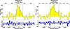 |
Fig. B.1. Spectra of the CO(3–2) toward SPT 0125-47 (left) and SPT 2134-50 (right) showing the coverage of the red and blue bins used to investigate the effect of differential lensing, as described in Section 4.1. In both cases, the spectrum is shown in the top panel, and the residuals from the Gaussian fit are shown in the bottom panel. The dashed blue line shows the two Gaussian fit to the spectra. The dashed gray line in the top panel and the shaded gray region in the lower panel indicate the per-channel RMS. Additionally, the top axis in the top panel of each spectrum displays the corresponding frequency. |
All Tables
All Figures
|
Fig. 1. Continuum image of SPT 0125-47 (top) and SPT 2134-50 (bottom). The contours are shown at −3, −2, 3, 4, 5σ levels. The synthesized beam is shown in the bottom left of each image. The black annulus shows the regions used to extract the dust continuum emission. |
| In the text | |
|
Fig. 2. Moment-0 and moment-1 maps of the CO(3–2) emission for SPT 0125-47 (top) and SPT 2134-50 (bottom). The first column shows the unmasked moment-0 map, the second column shows the moment-0 map masked to show only values above 3σ, and the third column shows the moment-1 map. The contours in the first two columns are shown at −3, −2, 3, 4, 5, 6, 7, 8, 9, 10σ levels. The synthesized beam is shown in the bottom left of each image. The black annulus in the unmasked moment-0 map for each source shows where the spectrum was extracted from. |
| In the text | |
|
Fig. 3. Spectra of the CO(3–2) toward SPT 0125-47 (left) and SPT 2134-50 (right). In both cases, the spectrum is shown in the top panel, and the residuals from the Gaussian fit are shown in the bottom panel. The dashed blue line shows the two Gaussian fit to the spectra. The dashed gray line in the top panel and the shaded gray region in the lower panel indicate the per-channel RMS. Additionally, the top axis in the top panel of each spectrum displays the corresponding frequency. |
| In the text | |
|
Fig. 4. Parametric (rows 1 and 3) and pixelized (rows 2 and 4) lens modeling of the CO(3–2) emission detected in SPT 0125-47 (top two rows) and SPT 2134-50 (bottom two rows). The first column displays the dirty image generated by PYAUTOLENS, with contours at −3, 3, 4, 5, 6, 7, 8, 9, 10σ levels. Note: this is not a cleaned image, so structures may differ slightly from those in cleaned images. The second column presents the dirty model image from PYAUTOLENS, also with contours at −3, 3, 4, 5, 6, 7, 8, 9, 10σ levels. The third column shows the dirty residual image produced by PYAUTOLENS, with contours at −3, 3, 4, 5σ levels. The fourth column illustrates the image plane emission parametric/pixelized model of the data, produced by PYAUTOLENS, with the black line representing the critical line. The fifth column shows the source plane emission parametric+pixelized model of the data from PYAUTOLENS, with the black line indicating the caustic line. All images are centered around the ALMA phase center. |
| In the text | |
|
Fig. 5. Source plane intensity (left), intensity error maps (middle), and S/N maps (i.e., intensity divided by intensity error, right) for SPT 0125-47 and SPT 2134-50. The gray polygons show the Voronoi mesh used for the pixelized reconstruction and the black line shows the caustic line. Both the intensity and intensity error maps are normalized, where the error maps have been normalized to the maximum of the intensity map, meaning that the value can be seen as a percentage error per pixel. The S/N map provides a measure of the significance of the reconstructed emission. |
| In the text | |
|
Fig. 6. Pixelized source plane models for the red and blue bins for SPT 0125-47, as described in Section 4.2.2 with source plane intensity (left), intensity error maps (middle), and S/N maps (i.e., intensity divided by intensity error, right). The gray polygons show the Voronoi mesh used for the pixelized reconstruction and the black line shows the caustic line. Both the intensity and intensity error maps are normalized, where the error maps have been normalized to the maximum of the intensity map, meaning that the value can be seen as a percentage error per pixel. |
| In the text | |
|
Fig. 7. Pixelized source plane models for the red and blue bins for SPT 2134-50 as described in Section 4.2.2 with source plane intensity (left), intensity error maps (middle), and S/N maps (i.e., intensity divided by intensity error: right). The gray polygons show the Voronoi mesh used for the pixelized reconstruction and the black line shows the caustic line. Both the intensity and intensity error maps are normalized, where the error maps have been normalized to the maximum of the intensity map, meaning that the value can be seen as a percentage error per pixel. |
| In the text | |
|
Fig. B.1. Spectra of the CO(3–2) toward SPT 0125-47 (left) and SPT 2134-50 (right) showing the coverage of the red and blue bins used to investigate the effect of differential lensing, as described in Section 4.1. In both cases, the spectrum is shown in the top panel, and the residuals from the Gaussian fit are shown in the bottom panel. The dashed blue line shows the two Gaussian fit to the spectra. The dashed gray line in the top panel and the shaded gray region in the lower panel indicate the per-channel RMS. Additionally, the top axis in the top panel of each spectrum displays the corresponding frequency. |
| In the text | |
Current usage metrics show cumulative count of Article Views (full-text article views including HTML views, PDF and ePub downloads, according to the available data) and Abstracts Views on Vision4Press platform.
Data correspond to usage on the plateform after 2015. The current usage metrics is available 48-96 hours after online publication and is updated daily on week days.
Initial download of the metrics may take a while.