| Issue |
A&A
Volume 705, January 2026
|
|
|---|---|---|
| Article Number | A119 | |
| Number of page(s) | 19 | |
| Section | Extragalactic astronomy | |
| DOI | https://doi.org/10.1051/0004-6361/202554950 | |
| Published online | 13 January 2026 | |
A constant pressure model for the warm absorber in Mrk 509
1
National Centre for Nuclear Research, Astrophysics Division Pasteura 7 02-093 Warsaw, Poland
2
Nicolaus Copernicus Astronomical Centre (NCAC), Polish Academy of Sciences Bartycka 18 Warsaw, Poland
3
CAS Key Laboratory for Research in Galaxies and Cosmology, Department of Astronomy, University of Science and Technology of China Hefei Anhui 230026, China
4
School of Astronomy and Space Science, University of Science and Technology of China Hefei Anhui 230026, China
5
European Space Agency (ESA), European Space Research and Technology Centre (ESTEC) Keplerlaan 1 2201 AZ Noordwijk, The Netherlands
★ Corresponding authors: This email address is being protected from spambots. You need JavaScript enabled to view it.
; This email address is being protected from spambots. You need JavaScript enabled to view it.
Received:
1
April
2025
Accepted:
21
October
2025
Abstract
Context. We present the analysis of 900 ks high-resolution RGS XMM-Newton observations of the nearby Seyfert galaxy Mrk 509 with the use of a self-consistent warm absorber (WA) model. We took a physically motivated approach to the modeling of the WA as a stratified medium in a constant total pressure (CTP) regime.
Aims. Powerful outflows are fundamental ingredients of any active galactic nucleus (AGN) structure. They can significantly affect the cosmological environment of their host galaxy. High-resolution X-ray data are best suited for outflow’s studies, and the observed absorption lines on heavy elements are evidence of the physical properties of an absorbing gas. Our models allow us to fit continuum shapes bounded together with the line profiles, which gives additional constraints on the gas structure of WA in this source. In this work, we benchmark and test the CTP model on the soft X-ray spectrum of Mrk 509.
Methods. A grid of synthetic absorbed spectra was computed with the photoionization code TITAN assuming that the system was under CTP. As an illuminating spectral energy distribution (SED), we used the most actual multiwavelength observations available for Mrk 509. We applied these models to the high-resolution spectrum of the WA in the Mrk 509, taking into account cold, warm and hot Galactic absorption on the way to the observer.
Results. The constant total pressure gas with log ξ0 ∼ 1.9, defined on the cloud surface, fits the data well. A higher ionization component is needed for Ne X absorption. The best-fit model is optically thin with log NH = 20.456 ± 0.016. The lines are non-saturated, and the CTP spectral fit aligns with previous analyses of Mrk 509 with a constant density WA. The model constrains the gas density, placing the WA cloud at 0.02 pc, consistent with the inner broad line region and the thickening region of the accretion disk.
Key words: galaxies: active / quasars: absorption lines / galaxies: Seyfert / quasars: individual: Mrk 509
© The Authors 2026
 Open Access article, published by EDP Sciences, under the terms of the Creative Commons Attribution License (https://creativecommons.org/licenses/by/4.0), which permits unrestricted use, distribution, and reproduction in any medium, provided the original work is properly cited.
This article is published in open access under the Subscribe to Open model. This email address is being protected from spambots. You need JavaScript enabled to view it. to support open access publication.
1. Introduction
Warm absorbers (WAs) are clearly seen in about 50% of active galactic nuclei (AGNs; Reynolds 1997; Blustin et al. 2005; Laha et al. 2014), and are direct candidates for explaining the feedback of the AGN to the galaxy and the intergalactic medium (IGM; Tombesi et al. 2013; Gofford et al. 2013). At the very beginning of the gratings detector area on the board of Chandra and XMM-Newton, X-ray spectra of ionized outflows in AGNs have been studied using the superposition of discrete gas components. However, it was recognized that this line richness from a variety of heavy elements requires the model resulting from photoionization calculations with some assumption about the matter structure. At that time, the reasonable assumption was that the absorbed gas is of constant density (CD; see Kaspi et al. 2001; Collinge et al. 2001; Kaastra et al. 2002; Behar et al. 2003; Netzer et al. 2003; Krongold et al. 2003; Yaqoob et al. 2003; Steenbrugge et al. 2003; Blustin et al. 2003, and many other papers).
So far, WAs have been fit by superposing the effect of CD slabs on different AGNs. However, since high-resolution spectra display lines from different levels of ionization, several CD slabs are needed to successfully explain the X-ray spectra (Turner et al. 2004; Steenbrugge et al. 2005; Costantini et al. 2007; Winter & Mushotzky 2010; Winter et al. 2012; Tombesi et al. 2013; Laha et al. 2014). To make clouds of different levels of ionization physically bounded, the more sophisticated model was provided by Różańska et al. (2004) assuming that the gas is under constant total pressure (CTP). In such a model, gas stratification is provided by a radiation pressure compression mechanism (see also Różańska et al. 2006, 2008; Stern et al. 2014).
The direct fitting of the line profile provides us with an estimate of the total energy absorbed by the line, the so-called line equivalent width (EW). After EWs of observed lines are found, and assuming that the observed lines are not saturated, we can derive the ionic column density of each ion responsible for the given line transition. This ionic column density for non-saturated lines is proportional to its EW, i.e., the linear part of the curve of growth (for illustration see: Adhikari 2019). This kind of work is made directly with the data and is the first step in the study of WAs. The second step is when, after deriving ionic column densities from the data, we can merge them with the total column density of the WA gas by fitting them with modeled ionic column densities computed by photoionization codes. These total column density, often expressed in terms of the hydrogen column density, may be different for each CD slab used in the data fitting process. The third step of the analysis is when we collect them into the so-called absorption measure distribution (AMD; Holczer et al. 2007; Behar 2009), allowing us to directly measure the strength of the absorption across the AGN outflow. After the AMD of several sources has been determined, it appeared that WAs have the broadest distributions of ionization among all absorbers observed in the Universe. Note that in the second stage of the above procedure, we can use more advanced photoionization models on the stratified density gas and try to reconstruct a continuous WA model, as has been done by several authors (Steenbrugge et al. 2005; Różańska et al. 2006; Costantini et al. 2007).
The more sophisticated WA model under CTP was directly fit to the data only in the case of high-resolution Chandra data of NGC 3783 (Gonçalves et al. 2006). For the purpose of that paper, photoionization calculations under CTP were made using the TITAN code (Dumont et al. 2003). And because in those days CTP models required significant computational power and time, they have been used to fit ionic column densities computed by TITAN to those derived by observations made by the Chandra X-ray observatory, i.e., the second stage of the whole procedure described above. It appeared that for NGC 3783 we cannot distinguish between CD and CTP models based on the relation of ionic column densities to the total column density of WA (Netzer et al. 2003; Gonçalves et al. 2006). Similar conclusions were drawn by Goosmann et al. (2016), whereby ionic column densities obtained by radiation pressure compressed cloud modeled with TITAN were nicely fit to the column densities observed of the particular ion, but the authors did not aim to reconstruct strong dips in AMD observed for NGC 3783.
On the other hand, CTP models of WA were successfully used to explain the AMD shapes observed in the case of several AGNs (Adhikari et al. 2015, 2019). This work was performed by estimating the AMD shape directly from the computed CTP models, without comparing the ionic column densities. The result was that AMD dips clearly observed in WAs are caused by thermal instabilities in the photoionized gas. Furthermore, the authors presented strong evidence that this gas has to be quite dense, with a density on the order of 1012 cm−3. The exception was Mrk 509, for which densities on the order of 108 cm−3 were sufficient to reconstruct AMD in this source (Adhikari et al. 2015). Since absorption models of gas under CTP predict dips in AMD that have been seen in the data (e.g. Behar 2009; Laha et al. 2016), CTP models should be more suitable to fit the observed lines directly to the X-ray spectra. A single CTP model of the gas with density stratification may account for several CD slabs. However, due to the complexity of model computations (as matter compressed by radiation can be thermally unstable) and spectral fitting (since multiple lines may not fit ideally), this work has never been done.
The ionized outflow in Mrk 509 is the one among several WAs that passed all the steps of the analysis described above. The source was observed by high-resolution gratings of XMM-Newton since 2000. The 600 ks observations taken between October and November 2009 were presented by Detmers et al. (2011, hereafter D11). They could successfully fit the high-resolution spectra taken by the Reflection Grating Spectrometer (RGS; den Herder et al. 2001) with a superposition of the components of the CD slab. After deriving ionic column densities for each of the ions behind the absorption line, they fit the ionization parameters and hydrogen column density of models which contribute to a given line or ion population. D11 concluded that the WA in Mrk 509 cannot be described by a smooth continuous AMD, but instead shows two strong discrete peaks. In addition, the authors concluded that there is no single model component that describes all the observed outflows. Furthermore, Adhikari et al. (2015) confirmed it on the basis of fitting AMD in the case of Mrk 509 with a CTP model.
Therefore, for the best observed source Mrk 509, there is a discrepancy in our understanding of the WA, and uncertainty over whether a contradictory physical description of the nature of the ionized outflow in Mrk 509 emerges from the direct estimate of the AMD, or from the fit of spectroscopic data with discrete CD components. On the basis of the AMD, the outflow can be continuous, but detailed spectral fitting of high-resolution X-ray data does not support this. To address this discrepancy, in this paper, we propose to revise the first step of the WA analysis for the source of Mrk 509, i.e., to fit the RGS spectra, presented in D11, in the CTP scenario, to understand what the origin is of this discrepancy and whether it comes from the model limitation or from the lack of our understanding of physical processes in the absorbing gas.
In this paper, we fit the CTP model directly to the high-resolution X-ray data, taking the information about the gas structure that we have learned from AMD analysis of the same source. Therefore, for the first time, the complete WA approach, i.e., estimating the column densities with CD components together with AMD derivation, is completed with the direct fitting of CTP photoionization model, in the case of one source. For this purpose, we prepared a grid of CTP TITAN models specifically computed for the Mrk 509 spectral energy distribution (SED) from the multiwavelength campaign of Kaastra et al. (2011). The ionic column densities and the EWs of lines are self-consistently derived from the fit model, and we can check if observed lines are saturated, i.e., on which branch of curve of growth the lines are placed (Adhikari 2019). For this work, we did not use exactly the same dataset as 600 ks data used by D11. Alternatively, we stacked together spectra extracted from observations covering the time range between 2000 and 2009 for a total exposure time of 900 ks.
The structure of the paper is as follows. In Sect. 2 we present the source and its WA prior observations. In Sect. 3 we describe the data and the reduction procedure used in this paper. The spectral model used for data fitting is described in Sect. 4, while the spectral analysis is presented in Sect. 5. Section 6 presents our results for fitting the total model. These results are discussed in Sect. 7 and concluded in Sect. 8.
2. Warm absorber in Mrk 509
Mrk 509 is a Seyfert 1.5 (Sy1.5) galaxy, also considered the closest quasar and Sy1 hybrid, and it harbors a supermassive black hole of mass 1.4 × 10⁸ M⊙ (Peterson et al. 2004). It is one of the best studied AGNs in the local Universe, with a redshift of 0.034397 (Huchra et al. 1993) and a high luminosity, L(1 − 1000 Ryd) = 3.2 × 1045 erg s−1, derived from the averaged broad-band SED observed in the multiwavelength campaign (Ebrero et al. 2011). Kaastra et al. (2011) published a very detailed broadband SED of Mrk 509, which was obtained by combining data from their multiwavelength observational campaign using XMM Newton. Moreover, their campaign also consisted of simultaneous data from INTEGRAL on hard X-rays, as well as Swift. The final SED was constructed including the infrared measurements from the IRAS and Spitzer data and is presented in Fig. 1 (red circles).
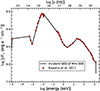 |
Fig. 1. Spectral energy distribution of Mrk 509 used as an input to the photoionization code TITAN marked as a solid black line. The red circles are the observational points reported by Kaastra et al. (2011) and normalized to the incident flux. |
Earlier work on the outflow in the X-ray regime has revealed that it consists of a wide range of ionization components but lacks a very high and also a very low ionized gas (weak Fe UTA and no Si XIV Lyα as reported by: Yaqoob et al. 2003). Usually, three outflow velocity components are needed to fully explain the observed absorption spectra (Smith et al. 2007, D11). Later, the X-ray outflow in this source has been extensively studied using the 600 ks RGS on board of the XMM-Newton X-ray telescope (Kaastra et al. 2011, 2012). The high spectral resolution of RGS allowed one to identify a few tens of absorption lines from highly ionized metals, and hence to determine their ionic column densities D11. Furthermore, multiple absorption lines from the interstellar medium were detected. Finally, to fully explain the RGS spectrum, several emission components were needed.
The above data allowed us to put new constraints on the WA in Mrk 509. D11 found that the ionized absorber consists of two velocity components, v = −13 ± 11 km s−1 and v = −319 ± 14 km s−1, which are consistent with previous results including UV data. Another tentative component, v = −770 ± 109 km s−1, is only seen in a few highly ionized absorption lines. However, several ionization components were assigned to each of the three velocity components. Thus, from the derived ionic column densities and with the use of photoionization calculations, D11 determined the equivalent hydrogen column densities and constructed the AMD. The authors demonstrated that the outflow in Mrk 509, in the log(ξ) range between 1 and 3 can be described by a broad function with two pronounced dips, whereby the column density drops by 2-3 orders of magnitude. Later, Adhikari et al. (2015) confirmed that such deeps are caused by thermal instability in the structure of the CTP cloud.
In addition, D11 showed that the highest ionization component is located at 0.5 pc, assuming that the observed changes in the absorption spectrum are due to the response to changes in the ionizing continuum with a delay related to the electron density. Kaastra et al. (2012) estimated the upper limits on the location of different ionization components of the WA in the range of 5 to 400 pc. All photoionization calculations performed by these authors were performed with the assumption of CD and the input SED determined for Mrk 509 from observations (Fig. 1).
3. Data reduction
We extracted observation data files (ODFs) for all the observations of Mrk 509 available in the public XMM-Newton archive1. They correspond to three separate campaigns performed in October 2001-April 2001, October 2005-April 2006, and October-November 2009. Data for each ODF were reduced using SASv16.0 (Gabriel et al. 2004), using the most updated calibration files available at the time of data reduction (October 2019). Calibrated event lists, source and background spectra, and response files (a combination of the redistribution matrix and of the energy-dependent effective area) were generated with the SAS reduction meta-task rgsproc. The reference position for the energy scale reconstruction was assumed at the optical coordinates of the AGN. rgsproc was run twice. The event lists generated in the first run were used to extract light curves of the CCD number 9 from a spatial region outside the dispersed source spectrum. In each light curve, intervals with a high particle background were identified as those corresponding to a count rate of > 2 s−1. In a second rgsproc run, the time intervals corresponding to the low particle background were used as inputs to select good events, from which the final scientific products were extracted.
Following D11, we combined the RGS 1 and RGS 2 spectra and responses generated in each observation with the SAS task rgscombine. The total exposure times are 903 and 900 ks for RGS 1 and RGS 2, respectively. In their analysis of the deep RGS observational campaign of Mrk 509, Kaastra et al. (2011) and D11 used the combined fluxed spectrum instead of the combined count spectrum, to avoid spurious narrow-band features that could arise at the wavelength of individual unexposed pixels because rgscombine combines the instrumental response without weighting (Kaastra et al. 2011). This issue could be exacerbated by the fact that the RGS was operated in “multi-pointing mode” during the 2009 observational campaign. However, fitting the fluxed spectrum introduces systematic uncertainties that are difficult to quantify because of the approximation required to correct the observed count spectrum for the instrumental response. The range of Mrk 509 count rates measured by the RGS is moderate (0.86–1.50 s−1 in the RGS 1 0.2–2.0 keV energy band, for example) except in the comparatively short 32 ks, Obs.#0130720101, which registered a RGS 1 count rate of 0.55 s−1 in the same energy band. We estimate that the systematic uncertainties potentially induced by the combination of the effective areas without weighting is ≤1.5%; that is, comparable to the systematic uncertainties in the calibration of the effective area (de Vries et al. 2015). In light of this result, we prefer to employ a rigorous forward-folding approach on the combined count spectra.
The above procedure allowed us to obtain a signal-to-noise ratio of the order of 10 on average, which is three times less than the signal-to-noise ratio reported by D11, after combining both RGS detectors. In order to prevent any additional lowness of the signal-to-noise ratio, we decided not to bin the data channels, even if the ftgrouppha tool from Heasoft ver. 6.25, with the option of optimal, indicates the saturation limit in the binning of high-resolution data (Kaastra & Bleeker 2016). For a visualization of the overall shape of the spectrum, we draw the data binned by five channels in Fig. 2.
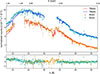 |
Fig. 2. Continuum model and Galactic absorption fit to Mrk 509 RGS spectrum. RGS 1 and RGS 2 spectra are plotted in orange and cyan. RGS 2 is arbitrarily shifted by 0.02 counts s−1 Å−1. The continuum model of Mrk 509 SED absorbed by the Milky Way is marked with continuous red and blue lines. The lower panel shows residuals against the best-fit model. The wavelengths are in the observed frame of reference. For the purpose of this plot the data are binned by five channels. |
4. Model description
We consider models of absorbing gas whereby radiation interacts with matter through photoionization processes. In this setup, we assume an ionizing continuum that illuminates a slab of gas in plane-parallel geometry. The gas is parameterized by the density of local numbers on the face of the cloud, nH, 0, and the total density of the columns, NH. The total pressure, which is the sum of the gas and radiation pressures, is assumed to be constant (CTP; Różańska et al. 2006). Our model differs from the radiation pressure compression model (Stern et al. 2014; Bianchi et al. 2019), since in the latter model, only the first order of radiation pressure decreasing proportionally to e−τ is taken into account, while the TITAN code computes the local value of the radiation pressure from the intensity field taking into account the current value of a source function (Adhikari 2019).
The ionization parameter, ξ0, in erg centimeter per second, is related to the ionizing flux by the following expression:
 (1)
(1)
where L is the incident luminosity integrated over the energy range available from observations (Kaastra et al. 2011), and r is the distance from the ionizing source. In the constant pressure regime, the values nH and ξ are strongly stratified across the inner layers of the slab, and we define them only at the cloud surface (Różańska et al. 2004, 2006). This is a static solution and does not account for the time evolution or the flow of matter.
A complete grid of models of the absorption spectra for WA was calculated with the TITAN code (Dumont et al. 2003; Chevallier et al. 2006). The code solves the transfer of radiation assuming the accelerated Lambda iteration (ALI) method, which takes into account the full treatment of the source function at each depth of the cloud and computes the line and continuum intensity self-consistently. A detailed description and advantages of the ALI method are described in Dumont et al. (2003) in the context of the X-ray absorber. The code computes self-consistently full profiles for absorption and emission lines and takes these profiles into account when doing radiative transfer computations. TITAN can also account for the effects of turbulence by setting the turbulent velocity value. The CTP medium for the purpose of Mrk 509 was illuminated with SED determined for this source from observations. The input SED for the TITAN code was taken from Kaastra et al. (2011, solid black line in Fig. 1).
The computed grid of ionizing parameters spans a range of 0 to 5 in log ξ0 with a 0.1 step and 20 to 23 in log NH with a 0.1 step. The upper limit of the column density was chosen on the basis of the shape of the absorbed continuum. For log NH > 23 the overall absorption of the continuum is high enough that it is inconsistent with the observed RGS continuum. We computed the table models for three initial volume densities on the illuminated face of the cloud: nH, 0 = 108, 1010, and 1012 cm−3. The choice of nH, 0 ≥ 108 cm−3 for the Mrk 509 absorber is motivated by the work of Adhikari et al. (2015), in which they demonstrated that the observed AMD for this source can be well reconstructed with the TITAN models for this gas density. In addition, the general shape of AMD for several sources is well reconstructed by high-density outflow (Adhikari et al. 2019).
The TITAN code fully takes into account the influence of turbulent velocity on the modeled line profile. The effect is illustrated in Fig. 3. It is clearly visible that turbulent velocity modifies the absorption line profile, as is expected from the theory of radiative transfer and the curve of growth analysis. Therefore, we have calculated all sets of models including turbulent velocities relevant to the values generally observed in other datasets, i.e., vturb = 100, 300, 500, and 700 km s−1. Note that turbulent velocities do not influence the shift of the location of the line centroids, which is caused by the outflow velocity. We did not fit the line shift individually; instead, the bulk shift was fit by using redshift for the absorption spectra as the independent parameter.
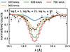 |
Fig. 3. Dependence of O VII profile on the turbulent velocities used in photoionization computations by the TITAN code for a given model. |
The number of ionic transitions taken into account is 4141 in the energy range between 0.01 eV and 25 keV. The ten most abundant elements are taken into account: H, He, C, N, O, Ne, Mg, Si, S, and Fe, with solar abundances following Grevesse & Anders (1989).
5. Spectral analysis
To analyze X-ray spectra, we used the software package Bayesian X-ray Analysis (BXA; Buchner et al. 2014, which connects the nested sampling algorithm MULTINEST (Feroz & Hobson 2008; Feroz et al. 2009, 2019) with the fitting environment XSPEC ver. 12.10.1 (Arnaud 1996). The procedure was performed in the energy range 0.326–1.550 keV (8–38 Å). In the process of evaluating the accuracy of the model, we used the goodness-of-fit statistic C-stat (Cash 1979), as it is implemented in XSPEC (Kaastra 2017). RGS 1 and RGS 2 were simultaneously fit, allowing only a cross-normalization factor to remain free in the fit (de Vries et al. 2015). We used uniform priors, so no preferences were given over the assumed parameter space.
In the first step, we fit the model of ionizing the SED without WA lines to have an initial point of reference for further improvements. The continuum model multiplied by Galactic absorption we used can be described as a product of components:
 (2)
(2)
where j is a number of Galactic absorption components, NH, Galj is the column density of neutral hydrogen in the Milky Way, σ is the cross section for absorption, and A is the normalization of the continuum. S(E) is the function that describes continuum radiation, which in our analysis is the SED of Mrk 509 that we used as the ionizing continuum in our photoionization computations.
As typical for AGNs, the complex absorption can be divided on external absorption connected to our Galaxy, for which the line redshift is almost zero, and intrinsic absorption is usually represented as a WA component, where the lines have the source redshift. As the first-order approximation of Galactic absorption, we used a single TBABS model with a fixed hydrogen column density value of 4.44 × 1020 cm−2 (Murphy et al. 1996). The overall model of the continuum absorbed by the Milky Way, fit to the data, is presented in Fig. 2. The model already displays several absorption lines due to the Milky Way gas.
To account for more complex, most likely multiphase Galactic absorption (Pinto et al. 2012), we also fit more advanced models: ISMABS (Gatuzz et al. 2015) and IONEQ (Gatuzz & Churazov 2018). The results of this fitting procedure are presented in Appendix A. The above analysis allowed us to identify several Galactic absorption lines in the data, given in Table A.3, which are later taken into account while identifying WA lines in Sect. 6.1. However, for further investigation of the WA components, we postponed the components ISMABS and IONEQ and relied exclusively on the model TBABS for Galactic absorption. This decision was motivated by prohibitive computing time in XSPEC with the Bayesian approach and, in some cases, failures in achieving the fit.
In addition, care was taken to identify instrumental features that may not be included in the response matrix of the RGS. The instrumental lines, together with the references, are listed in Table A.4.
Subsequently, on the top of the continuum modified by Galactic absorption, we added ionized CTP components to the product of models:
 (3)
(3)
where i is a number of components of the WA and each WAi(NH, i, ξi) is parameterized with the column density and the ionization parameter. To be in agreement with AMD fitting, only one CTP component should be needed to fit the data; that is, i = 1.
The overall, major fit components are listed in Table 1, where in the third row we describe the best-fit parameters of a single CTP model with solar abundances. The model requires a turbulent velocity equal to 500 km s−1.
Best-fit parameters of the final model.
6. The results of fitting the total model
In the following, we discuss our final fit model with its physical implications. The overall spectral fit for both RGS data, which includes continuum emission multiplied by Galactic absorption, and multiplied by the single CTP WA model, is presented in Fig. 4. The best-fit parameters are described in Table 1.
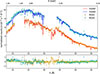 |
Fig. 4. Warm absorber on top of continuum modified by Galactic absorption with Mrk 509 RGS data points. RGS 1 and RGS 2 spectra are plotted in orange and cyan. RGS 2 is arbitrarily shifted by 0.02 counts s−1 Å−1. The total model consisting of continuum together with a single CTP WA is plotted in red and blue. The wavelengths are in the observed frame of reference. The lower panel shows residua. For the purpose of this plot the data are binned by five channels. |
We point out here that our continuum emission has the shape of an observed SED and was not corrected for unknown intrinsic absorption. In the work of Detmers et al. (2011), the same continuum was used, but the lines were fit separately as absorption of the ion population. The approach of the authors described above is similar to using absorption lines on top of the incident continuum. Our model computations allow us to use the so-called “outward” spectrum, which is the result of the incident spectrum corrected by absorption.
Thus, in our approach, the best-fit model for the continuum is a multiplication of the CTP WA model by the incident continuum SED with 100% coverage, and it is presented in Fig. 4. More consistent additive models, where the sum of the incident and outward models (and optionally reflection) is fit, give an overall good fit but do not fit so well the O VIIIλ ∼ 19.6 Å and O VIIλ ∼ 22.33 Å lines in the global solution. Weaker lines in the global fit of the additive solution are probably caused by the fact that the incident component is stronger than the outward component to preserve a good overall fit of the continuum. This is interpreted as a lower covering factor of the absorber. But this destroys fit in the deeper lines profiles. Thus, we conclude that the true incident continuum should be softer with a higher level of flux density above 25 Å (below 0.5 keV). Having this in mind, we decided to stay with the original input SED, even if our fit is not perfect. However, since we do not have any better constraints on the shape of the continuum, we have chosen to use the original SED, which allows the comparison of our results with the previous work.
The Galactic column density of our overall fit model with component TBABS is NH = 4.44 × 1020 cm−2, and it is kept frozen during spectral analysis (Murphy et al. 1996; Willingale et al. 2013). It should be noted that the above value is 0.5 higher than that found by HI4PI Collaboration (2016).
We made the initial choice of the best nH, 0 by comparing independent fits of the models and assessing their fit quality. For each of nH, 0 = 108, 1010, and 1012 cm−3, we fit the overall absorption spectrum in the parameter space log ξ0–log NH. The best statistic was obtained for nH, 0 = 1010 cm−3, although the advantage over 108 cm−3 was rather minor, on the order of a few hundred in the c-stat value. This consideration is also in line with the conclusion that AMD analysis does not exclude models with gas density 1010 cm−3 (see Fig. 14, Adhikari et al. 2019). Thus, we proceeded further with our analysis with the model assuming nH, 0 = 1010 cm−3.
In a similar fashion, we made a choice for the turbulent velocity in the model. From the calculated grids with vturb = 100, 300, 500 and 700 km s−1, we chose the velocity for which the best value of c-stat was obtained. Effectively vturb increases the depth of absorption for the given ξ, NH, and nH, 0, as is illustrated in Fig. 3. The best result was achieved for vturb = 500 km s−1.
The parameters of the best-fit WA model are:  , log NH = 20.456 ± 0.016. The fit values with their errors are interpolated values as given by the BXA package, while the grid step was 0.1 in both parameters, and this value defines a potentially more realistic precision of the solution. The overall fit statistic in our analysis is worse than the one obtained by D11, but a direct comparison of the statistics is not possible. On the one hand, we did not add both RGS spectra, allowing for the lower statistic, but on the other hand, we did not bin the data in order to keep all lines visible even on the detection limit. In addition, our model is also more tight, since the entire photoionization component in the CTP regime fits all lines for a given ionization parameter on the cloud surface (Adhikari et al. 2019). Alternatively, D11 needed 5-6 CD components to model lines from different ionization states of heavy elements, and such an approach is much more flexible in terms of the goodness of fit.
The ionization parameter on the cloud surface, ξ0, resulting from our fitting is relatively low, log ξ = 1.98, and decreases as the depth of the WA cloud increases, as is presented in the upper panel of Fig. 6. The temperature and density structure given in the lower panels directly follow this change. The illuminated cloud surface is on the right side of Fig. 6. Even if ionization is stratified in our model, it does not reflect the high-ionization CD components fit by D11. Our WA of best fit is optically thin with a total column density of log NH = 20.456. The first reason for this fact is that, in a CTP regime, ionization fronts are very narrow, and with only a minor change in temperature and density, we jump to a different ionization state when lines appear. It is worth pointing out that the resulting values of the temperature of the stratified WA are outside the regime where typical thermal instability occurs.
The second reason is that the collected RGS data cover a very narrow energy range, i.e., 0.34–1.5 keV, and the data cannot fully reflect the highly ionized CTP phase. For the same reason, the broad distribution of ionization, which manifests itself in an AMD constructed with the use of CD slabs, can be modeled only by a relatively narrow optically thin CTP model. A new high-resolution detector with energy coverage up to 10 keV, such as the X-IFU instrument (Barret et al. 2023) on the board of the future New-Athena mission, is needed to account for the optically thick WA consisting of low- and high-ionization zones in the single CTP model (Różańska et al. 2008).
Figure 5 shows the confidence contours generated by BXA between different parameters of the WA CTP model that best fits. The cross normalization factor between the RGS 1 and RGS 2 spectra is very well constrained to a value of 0.98. A small degeneracy between normalization and the total column density is observed, but otherwise parameter values are robustly constrained. This suggests that our fit is acceptable for further analysis.
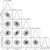 |
Fig. 5. BXA contour plots for fit parameters of the total model to the Mrk 509 RGS 1 and RGS 2 spectra. The cross-normalization factor shows the difference between two RGS specra where normalization gives the position of the total model. Best fit log |
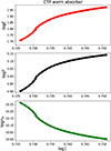 |
Fig. 6. Ionization structure of the best-fit CTP model computed by TITAN and fit to the Mrk 509 RGS data. The upper panel shows the structure of ionization parameter ξ, the medium panel the temperature, T (S-curve), and the bottom panel the volume density, nH, all versus the dynamical ionization parameter, Ξ. The illuminated cloud surface is located on the right side of the panels. |
For many years, the dependence of photoionization models on the gas volume density was thought to be degenerate, i.e., the absorbed spectra were the same for wide ranges of the gas density. But this conclusion was valid for early studies of optical absorption lines from nebulae, where the physical conditions of matter required low-density gas, on the order of ∼104 cm−3. For this reason, CD models were generally accepted in publicly available photoionization codes. But with the increasing sensitivity of spectrometers, it appeared that this was indeed true for optically thin clouds, with a total thickness of less than 1, and for nonsaturated clouds. In the case of AGNs, observed in either the optical/UV or X-ray range, very often lines are saturated, and the gas with an optical depth larger than unity is needed to explain all absorption features. The first brake to the degeneracy of photoionization models due to gas density was presented by Różańska et al. (2008) in the case of WAs in AGNs. In addition, it was broadly discussed by Adhikari (2019), where the direct physical reason for such behavior was provided.
Today, we accept that for volume densities higher than ∼106 − 8 cm−3, depending on the shape of the illuminating broadband continuum, outgoing radiation depends not only on the ionization parameter and column density, but also on the volume density of the gas. Since our model depends on many parameters, it was not possible to fit directly the volume density of the gas at the cloud surface. We clearly demonstrated that AMD for Mrk 509 can be well reproduced for a gas density of about 108 cm−3 (Adhikari et al. 2015).
For the goal of this paper, we computed models for various values of the gas density at the cloud surface and microturbulence. Since those models were huge, it imposed serious problems while we were using it in XSPEC with the Monte Carlo fitting method. Thus, we decided to omit direct fitting of nH, 0 and turbulence. We only compared best-fit solutions for log nH, 0: 8, 10, and 12. The best C-stat was achieved for a value of 10, although the difference was small. After fixing the gas density, we proceeded in a similar way with turbulence, choosing 500 km s−1 as preferred. Therefore, the gas density and turbulence were not fully fit but weakly constrained. We accept 1010 cm−3 as the preferred density for which other parameters, such as the ionization parameter and the column density, give an acceptable fit.
We obtained this best fit for nH, 0 = 1010 cm−3, which places our WA cloud at a distance of 0.02 pc, using the fit value of the ionization parameter and the source luminosity of Sect. 2. This distance is a factor of 4 higher than our earlier finding (Adhikari et al. 2015; Adhikari 2019), but it is in agreement with the location of the broad line region found in the reverberation mapping. We suggest here that such WA can be connected with a BLR gas of lower temperature and can be responsible for additional continuum emission observed by RGS detectors.
6.1. WA lines
To take a closer look at our analysis, we focus on different spectral bands, presenting the overall best-fit model together with the data in the observed frame in Figs. from A.1 to A.1. Both RGS spectra were fit simultaneously with parameters listed in Table 1. The prominent absorption lines resulting from several ions of Mg, Ne, Fe, O, N, and C are presented in the figures. All lines associated with WA are identified with black labels, whereas those associated with Galactic absorption are identified with green labels. Lines that appear in RGS 1 and are not detected by RGS 2 are probably associated with instrumental lines. The instrumental lines that are included in the response matrix of both gratings are listed in Table A.4.
The identification of absorption lines due to the WA medium in AGNs is associated on the basis of known atomic data of X-ray transitions. There has been a long-standing discussion about a common database of atomic transitions, but to date it does not exist, and the data may differ slightly in various theoretical models. In general, our identification of lines is almost the same as in D11, with small exceptions of several transitions, which are located very close to each other on the energy scale. Such blended lines are difficult to disentangle with the current resolution of X-ray data. All lines associated with WA and identified by us are listed in Table 2.
Absorption lines due to the WA in Mrk 509 identified with CTP model.
To find the optimal parameters of the model and reproduce prominent lines, a test was prepared. The spectra were divided into windows that contained prominent absorption lines. The model of log nH, 0 = 10, vturb = 500 km s−1, and a solar abundance was used (warm500). Spectral windows were named lwxx, where xx denotes the integer wavelength value contained in the window. Most of the fits in these spectral windows achieve a c-stat per d.o.f. in the range 1.2 − 1.8. The fitting parameters are also illustrated in Fig. 7. We see that the best fit of the entire spectrum with a single absorber marked with a red star is located in the middle of log ξ. However, the total column density is low to avoid stronger absorption that is not visible in the spectrum and preserve a good fit of the continuum. As a consequence of the low total column density, the lines are non-saturated; therefore, both CTP and CD models may successfully reproduce the data.
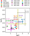 |
Fig. 7. Best-fit parameters using spectral windows with warm500 multiplicative model. |
We calculated the velocity shift of the WA lines (average value of the prominent absorption lines) to be v = −197 [km s−1] (blueshift caused by an outflow) in the rest-frame. These values are presented in Table 1. We adopted the hydrogen number density nH, 0 = 1010 cm−3. Moreover, given our low column density in the TITAN calculations and with a high gas density, we never went through a general stratification of the ionization parameter. This is one of the reasons why we do not have a full S-curve, as is seen from the middle panel of Fig. 6.
7. Discussion
We performed an analysis of high-resolution RGS XMM-Newton data from Mrk 509 with a model of a stratified medium in the CTP regime. Our data reduction procedure allowed us to collect 900 ks observations – the longest possible for this source. Both RGSs have been fit simultaneously, and we have taken care of proper data binning without a loss of spectral resolution.
Our results are comparable to those obtained during the most detailed fit of the absorption spectra of Mrk 509 published by D11. The authors fine-tuned the input ionizing continuum and describe it with splines to achieve a better match in the spectra. Here we used the same SED as D11, following the work of Kaastra et al. (2011). However, we incorporated a slightly different dataset, RGS observations collected over the longer period. This is potentially the source of the short-wavelength part difference.
D11 conducted a very detailed fitting of the absorption lines in the Mrk 509 spectrum. This allowed reconstructing smooth AMD made up of many layers responsible for the effective creation of different absorption lines. However, they concluded that the absorption spectrum can be reasonably and accurately approximated with the five CD slabs model. These components are spread over the scale of ionization parameters; log ξ: −0.14, 0.81, 2.03, 2.2, 2.62, and 3.26 for their model 3 (their table 6). The corresponding values of the column density of the slabs are: 19.6, 19.9, 20.41, 20.64, 20.25, and 20.8 in logarithm of inverse square centimeter. While Ebrero et al. (2011) found log ξ: 1.06, 2.26, 3.15 with log column densities: 20.3, 20.7, 20.8 by fitting soft X-ray spectrum taken with Chandra.
Our best-fit static CTP model with the fit parameters:  and log NH = 20.456 ± 0.016 for a WA outflow with v = 195 ± 16 km s−1 is slightly worse than that of D11, but is satisfactory for most of the lines, and the overall fit looks good with C-stat per d.o.f. = 1.9. Nevertheless, we have checked that for our model and these particular datasets, increasing CTP model components (i.e., increasing i) does not improve our fit considerably, only by a few C-stat. Therefore, we refrained from adding additional WA model components, because it only complicates our analysis, and therefore only a single CTP model is discussed here. However, the single model was dominant in most of the absorption lines except the Ne X line. One thing is the velocity gradient between different absorption lines, which limits the fit quality of a single static photoionization model. The velocity shift issue could be resolved by adding more shifted components between each other, but the expected improvement was small. The ultimate difficulty was that with the assumed ionizing continuum as in D11, improving all prominent lines at once causes the emergence of additional absorption, which destroyed the continuum fit in the absorption line-free area. This was caused by the need to increase the column density in a larger ξ space (addressing Ne X, as in the solution “lw12”). It should be noted that we do not address a cooler medium below 104 K in our model.
Our solution, which is not as good as Detmer’s, is, however, close in terms of the ionization parameters and column densities. Our S-curve is also similar. The main difference is that the solutions computed in TITAN reside in Ξ lower than the solutions proposed by D11 for the corresponding values of ξ. Ξ is the dynamical ionization parameter and is defined as Ξ ≡ Prad/Pgas, where Prad is the radiation pressure and Pgas is the gas pressure. The difference is around −0.2 in log Ξ for models with log nH, 0 = 8 on the face of the cloud. The difference is greater, around −0.4, for log nH, 0 = 12. However, there are a few differences in our approach, such as the use of a different ionization code, slightly different abundances and atomic data, a dataset covering a broader time span without binning, and fitting two detector spectra at once.
To address the issue of a few unfit lines and recheck those that were fit, we repeated the fitting using narrower windows containing individual strong absorption lines. The results of this procedure are presented in Fig. 7. It shows that, in fact, the optimal ionization parameters might be spread over a range of values from 0.5 to 3.5 in log ξ. Although huge error bars are present for some lines indicating that a broad range of ionization parameter is possible (such as for N VII in lw28). The problem here is that the windows are narrow and do not address the impact of the absorbing cloud on the whole continuum. For several lines, the “optimal” column density is large, and affected continuum matches outside of a given window. This is the reason why the overall fitting does not reach higher column densities. However, the results in Fig. 7 seem to be consistent with the solution of D11 and Ebrero et al. (2011).
We can place our WA cloud at a distance of 0.02 pc or 6 × 1016 cm, using the fit value of the ionization parameter, nH, 0 = 1010 cm−3, and the source luminosity. This value indicates the overdensity in the atmosphere of the accretion disk and the thickening of the disk (Adhikari et al. 2018). That would be close to the inner broad line region position. However, it is much smaller than the limits proposed by Ebrero et al. (2011), Kaastra et al. (2012), who estimated from the X-ray spectra modeling that the absorber should be farther than 5 pc, because of its size-radius constraint. However, based on ionization parameter variability Kaastra et al. (2012) suggested an upper limit of 0.5 pc, which would be consistent with our estimate.
7.1. Ne X fitting issue
This global solution is not able to reproduce Ne lines – especially Ne X, which is optimally fit with a higher ionization parameter and column density. Fitting in the window spanning from 12.3 up to 12.7 Å (model “lw12”) gives good results. Ne X
λ ∼ 12.5 Å is possible to fit for a model with log ξ > 1.8 and log NH > 21.1. The exact values depend on the configuration of the additional components (such as reflection). The region of the Ne X line is plotted in Fig. 8, where we see two solutions that reproduce the line: orange and green, while the best global solution is plotted in blue. Orange is for the multiplicative model with the incident continuum fit in lw12 window, which gives log ξ = 2.79 and log NH = 21.17; green shows the additive model with reflection fit in lw12 window, where the absorption and reflection parameters are log  and log
  . However, what these two models have in common, in contrast to the global solution, is primarily a higher column density and a blueshift on the order of 1000 km s−1. Meanwhile, fitting other lines and/or reflection requires lower shifts.
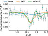 |
Fig. 8. Spectrum in the wavelength range of 12.3–12.7 Å containing Ne X line. |
Ebrero et al. (2011) concluded that their low log ξ ∼ 1 component is not in pressure equilibrium with the other two, which are more ionized. In principle, they did not directly reject the possibility of the coexistence of the log ξ = 2.3 and log ξ = 3.2 solutions being in pressure equilibrium. Our single cloud solution gives a good overall fit and is consistent with the log ξ ∼ 2 medium. However, the problem with reproducing Ne X absorption and the fact that it is more shifted than the oxygen lines indicate that a more complex model is needed. A second component or a dynamic model that accounts for medium expansion is likely required.
It was tempting to test whether a continuous AMD (Adhikari et al. 2015) could be reproduced by directly fitting the spectrum with a single CTP model. However, this was not possible with direct fitting of a single static CTP model. One of the key issues was the gradient in the line shifts, which suggests that dynamics must be addressed in physically motivated models.
7.2. Emission
D11 identified emission features as radiative recombination continua, the most prominent around 22–24 Å from the O VII lines. Our trials with using the reflection spectrum over the same TITAN grid as the absorption one did not improve the fit. The sharp emission lines present in the model appeared in a broad range of wavelengths. It was necessary to broaden the emission spectrum. The flux excess could potentially be addressed only by a smeared reflection. However, our attempt to apply a smeared reflection component also does not improve the fit globally. Since our reflection spectra show emission lines in a broader range of wavelengths, optimizing the fit solution resulted in negligible emission model amplitude. However, locally emission indeed improved the fit, as in the Ne X window presented in Fig. 8. It is possible that the illuminating continuum that is used in our case may not represent the total spectrum seen by the absorber. Since it is implemented, the continuum is a spline that incorporates bumps into the continuum. It is possible that as a result the possible flux excess coming from a smeared emission is incorporated into the assumed continuum. Fitting the reflection from TITAN would require us to revisit the ionizing continuum and recompute the grid. This is beyond the scope of this work.
8. Conclusions
The CTP model with  and log NH = 20.456 ± 0.016 for the WA outflow with velocity v = 195 ± 16 km s−1, as presented in our work, provides a good general fit to the XMM RGS data. We found that a static CTP model does not address all WA absorption lines with a single component. This is due to the fact that it does not include the velocity gradient across the slab, and thus does not fit gradual line shift with the ionization parameter. Although preserving the apparent continuum shape in the fit does not allow us to increase the column density above log NH ∼ 20.5, an additional component with log ξ ∼ 3 is required to account for Ne X absorption, which is consistent with the conclusions in the literature (Ebrero et al. 2011, D11).
We conclude that the CTP model is applicable, while more self-consistent than CD models, and is more straightforward to interpret. We were unable to reproduce a continuous AMD by a direct fit of the single static CTP model, most probably because of the dynamics of the observed medium.
Acknowledgments
We are grateful to the anonymous referee for his/her comments that improved our paper. The authors thank Alex Markowitz for helpful discussion. This research was partially supported by the Polish National Science Center grant No. 2021/41/B/ST9/04110. TPA acknowledges the support from the National Natural Science Foundation of China (nos. 12222304, 12192220, and 12192221).
References
- Adhikari, T. P. 2019, Photoionization Modelling as a Density Diagnostic of Line Emitting/Absorbing Regions in Active Galactic Nuclei (Cham: Springer International Publishing) [Google Scholar]
- Adhikari, T. P., Różańska, A., Sobolewska, M., & Czerny, B. 2015, ApJ, 815, 83 [NASA ADS] [CrossRef] [Google Scholar]
- Adhikari, T. P., Hryniewicz, K., Różańska, A., Czerny, B., & Ferland, G. J. 2018, ApJ, 856, 78 [NASA ADS] [CrossRef] [Google Scholar]
- Adhikari, T. P., Różańska, A., Hryniewicz, K., Czerny, B., & Behar, E. 2019, ApJ, 881, 78 [NASA ADS] [CrossRef] [Google Scholar]
- Arnaud, K. A. 1996, in Astronomical Data Analysis Software and Systems V, eds. G. H. Jacoby, & J. Barnes, ASP Conf. Ser., 101, 17 [NASA ADS] [Google Scholar]
- Barret, D., Albouys, V., Herder, J.-W. d. et al. 2023, Exp. Astron., 55, 373 [NASA ADS] [CrossRef] [Google Scholar]
- Behar, E. 2009, ApJ, 703, 1346 [NASA ADS] [CrossRef] [Google Scholar]
- Behar, E., Rasmussen, A. P., Blustin, A. J., et al. 2003, ApJ, 598, 232 [Google Scholar]
- Bianchi, S., Guainazzi, M., Laor, A., Stern, J., & Behar, E. 2019, MNRAS, 485, 416 [NASA ADS] [CrossRef] [Google Scholar]
- Blustin, A. J., Branduardi-Raymont, G., Behar, E., et al. 2003, A&A, 403, 481 [NASA ADS] [CrossRef] [EDP Sciences] [Google Scholar]
- Blustin, A. J., Page, M. J., Fuerst, S. V., Branduardi-Raymont, G., & Ashton, C. E. 2005, A&A, 431, 111 [CrossRef] [EDP Sciences] [Google Scholar]
- Buchner, J., Georgakakis, A., Nandra, K., et al. 2014, A&A, 564, A125 [NASA ADS] [CrossRef] [EDP Sciences] [Google Scholar]
- Cash, W. 1979, ApJ, 228, 939 [Google Scholar]
- Chevallier, L., Collin, S., Dumont, A. M., et al. 2006, A&A, 449, 493 [NASA ADS] [CrossRef] [EDP Sciences] [Google Scholar]
- Collinge, M. J., Brandt, W. N., Kaspi, S., et al. 2001, ApJ, 557, 2 [Google Scholar]
- Costantini, E., Kaastra, J. S., Arav, N., et al. 2007, A&A, 461, 121 [CrossRef] [EDP Sciences] [Google Scholar]
- de Vries, C. P., den Herder, J. W., Gabriel, C., et al. 2015, A&A, 573, A128 [NASA ADS] [CrossRef] [EDP Sciences] [Google Scholar]
- den Herder, J. W., Brinkman, A. C., Kahn, S. M., et al. 2001, A&A, 365, L7 [NASA ADS] [CrossRef] [EDP Sciences] [Google Scholar]
- Detmers, R. G., Kaastra, J. S., Steenbrugge, K. C., et al. 2011, A&A, 534, A38 [NASA ADS] [CrossRef] [EDP Sciences] [Google Scholar]
- Dumont, A.-M., Collin, S., Paletou, F., et al. 2003, A&A, 407, 13 [NASA ADS] [CrossRef] [EDP Sciences] [Google Scholar]
- Ebrero, J., Kriss, G. A., Kaastra, J. S., et al. 2011, A&A, 534, A40 [NASA ADS] [CrossRef] [EDP Sciences] [Google Scholar]
- Feroz, F., & Hobson, M. P. 2008, MNRAS, 384, 449 [NASA ADS] [CrossRef] [Google Scholar]
- Feroz, F., Hobson, M. P., & Bridges, M. 2009, MNRAS, 398, 1601 [NASA ADS] [CrossRef] [Google Scholar]
- Feroz, F., Hobson, M. P., Cameron, E., & Pettitt, A. N. 2019, Open J. Astrophys., 2, 10 [Google Scholar]
- Gabriel, C., Denby, M., Fyfe, D. J., et al. 2004, in The XMM-Newton SAS - Distributed Development and Maintenance of a Large Science Analysis System: A Critical Analysis, eds. F. Ochsenbein, M. G. Allen, & D. Egret, ASP Conf. Ser., 314, 759 [Google Scholar]
- Gatuzz, E., & Churazov, E. 2018, MNRAS, 474, 696 [NASA ADS] [CrossRef] [Google Scholar]
- Gatuzz, E., García, J., Kallman, T. R., Mendoza, C., & Gorczyca, T. W. 2015, ApJ, 800, 29 [NASA ADS] [CrossRef] [Google Scholar]
- Gatuzz, E., García, J. A., Kallman, T. R., & Mendoza, C. 2016, A&A, 588, A111 [NASA ADS] [CrossRef] [EDP Sciences] [Google Scholar]
- Gofford, J., Reeves, J. N., Tombesi, F., et al. 2013, MNRAS, 430, 60 [Google Scholar]
- Gonçalves, A. C., Collin, S., Dumont, A. M., et al. 2006, A&A, 451, L23 [NASA ADS] [CrossRef] [EDP Sciences] [Google Scholar]
- Gonzalez-Riestra, R. 2018, XMM [Google Scholar]
- Goosmann, R. W., Holczer, T., Mouchet, M., et al. 2016, A&A, 589, A76 [NASA ADS] [CrossRef] [EDP Sciences] [Google Scholar]
- Grevesse, N., & Anders, E. 1989, in Cosmic Abundances of Matter, ed. C. J. Waddington, AIP Conf. Ser., 183, 1 [Google Scholar]
- Holczer, T., Behar, E., & Kaspi, S. 2007, ApJ, 663, 799 [NASA ADS] [CrossRef] [Google Scholar]
- HI4PI Collaboration (Ben Bekhti, N., et al.) 2016, A&A, 594, A116 [NASA ADS] [CrossRef] [EDP Sciences] [Google Scholar]
- Huchra, J., Latham, D. W., da Costa, L. N., Pellegrini, P. S., & Willmer, C. N. A. 1993, AJ, 105, 1637 [NASA ADS] [CrossRef] [Google Scholar]
- Kaastra, J. S. 2017, A&A, 605, A51 [NASA ADS] [CrossRef] [EDP Sciences] [Google Scholar]
- Kaastra, J. S., & Bleeker, J. A. M. 2016, A&A, 587, A151 [NASA ADS] [CrossRef] [EDP Sciences] [Google Scholar]
- Kaastra, J. S., Steenbrugge, K. C., Raassen, A. J. J., et al. 2002, A&A, 386, 427 [NASA ADS] [CrossRef] [EDP Sciences] [Google Scholar]
- Kaastra, J. S., de Vries, C. P., Costantini, E., & den Herder, J. W. A. 2009, A&A, 497, 291 [NASA ADS] [CrossRef] [EDP Sciences] [Google Scholar]
- Kaastra, J. S., Petrucci, P.-O., Cappi, M., et al. 2011, A&A, 534, A36 [NASA ADS] [CrossRef] [EDP Sciences] [Google Scholar]
- Kaastra, J. S., Detmers, R. G., Mehdipour, M., et al. 2012, A&A, 539, A117 [NASA ADS] [CrossRef] [EDP Sciences] [Google Scholar]
- Kaastra, J. S., de Vries, C. P., & den Herder, J. W. 2018, SRON [Google Scholar]
- Kaspi, S., Brandt, W. N., Netzer, H., et al. 2001, ApJ, 554, 216 [NASA ADS] [CrossRef] [Google Scholar]
- Krongold, Y., Nicastro, F., Brickhouse, N. S., et al. 2003, ApJ, 597, 832 [NASA ADS] [CrossRef] [Google Scholar]
- Laha, S., Guainazzi, M., Dewangan, G. C., Chakravorty, S., & Kembhavi, A. K. 2014, MNRAS, 441, 2613 [NASA ADS] [CrossRef] [Google Scholar]
- Laha, S., Guainazzi, M., Chakravorty, S., Dewangan, G. C., & Kembhavi, A. K. 2016, MNRAS, 457, 3896 [NASA ADS] [CrossRef] [Google Scholar]
- Murphy, E. M., Lockman, F. J., Laor, A., & Elvis, M. 1996, ApJS, 105, 369 [NASA ADS] [CrossRef] [Google Scholar]
- Netzer, H., Kaspi, S., Behar, E., et al. 2003, ApJ, 599, 933 [NASA ADS] [CrossRef] [Google Scholar]
- Nicastro, F., Senatore, F., Gupta, A., et al. 2016, MNRAS, 457, 676 [NASA ADS] [CrossRef] [Google Scholar]
- Peterson, B. M., Ferrarese, L., Gilbert, K. M., et al. 2004, ApJ, 613, 682 [Google Scholar]
- Pinto, C., Kriss, G. A., Kaastra, J. S., et al. 2012, A&A, 541, A147 [NASA ADS] [CrossRef] [EDP Sciences] [Google Scholar]
- Reynolds, C. S. 1997, MNRAS, 286, 513 [NASA ADS] [CrossRef] [Google Scholar]
- Różańska, A., Czerny, B., Siemiginowska, A., Dumont, A. M., & Kawaguchi, T. 2004, ApJ, 600, 96 [Google Scholar]
- Różańska, A., Goosmann, R., Dumont, A.-M., & Czerny, B. 2006, A&A, 452, 1 [NASA ADS] [CrossRef] [EDP Sciences] [Google Scholar]
- Różańska, A., Kowalska, I., & Gonçalves, A. C. 2008, A&A, 487, 895 [NASA ADS] [CrossRef] [EDP Sciences] [Google Scholar]
- Smith, R. A. N., Page, M. J., & Branduardi-Raymont, G. 2007, A&A, 461, 135 [NASA ADS] [CrossRef] [EDP Sciences] [Google Scholar]
- Steenbrugge, K. C., Kaastra, J. S., de Vries, C. P., & Edelson, R. 2003, A&A, 402, 477 [NASA ADS] [CrossRef] [EDP Sciences] [Google Scholar]
- Steenbrugge, K. C., Kaastra, J. S., Crenshaw, D. M., et al. 2005, A&A, 434, 569 [NASA ADS] [CrossRef] [EDP Sciences] [Google Scholar]
- Stern, J., Behar, E., Laor, A., Baskin, A., & Holczer, T. 2014, MNRAS, 445, 3011 [NASA ADS] [CrossRef] [Google Scholar]
- Tombesi, F., Cappi, M., Reeves, J. N., et al. 2013, MNRAS, 430, 1102 [Google Scholar]
- Turner, A. K., Fabian, A. C., Lee, J. C., & Vaughan, S. 2004, MNRAS, 353, 319 [NASA ADS] [CrossRef] [Google Scholar]
- Willingale, R., Starling, R. L. C., Beardmore, A. P., Tanvir, N. R., & O’Brien, P. T. 2013, MNRAS, 431, 394 [Google Scholar]
- Winter, L. M., & Mushotzky, R. 2010, ApJ, 719, 737 [Google Scholar]
- Winter, L. M., Veilleux, S., McKernan, B., & Kallman, T. R. 2012, ApJ, 745, 107 [NASA ADS] [CrossRef] [Google Scholar]
- Yaqoob, T., McKernan, B., Kraemer, S. B., et al. 2003, ApJ, 582, 105 [Google Scholar]
Obs.#0130720101, #0130720401, #0306090101, #0306090201, #0306090301, #0306090401, #0601390201, #0601390301, #0601390401, #0601390501, #0601390701, #0601390801, #0601390901, #0601391001, #0601391101.
Appendix A: Absorption lines of an external origin
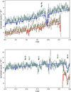 |
Fig. A.1. Overall model fit to Mrk 509 RGS spectrum given in observed frame. RGS 1 and RGS 2 spectra are plotted in orange and cyan dots with arbitrary shift 0.02 counts s−1 Å−1, and errors marked by gray bars. The total model: continuum together with single CTP WA is plotted in red and blue. WA lines are identified with black text, while possible absorption lines on Milky Way - by green text. For instrumental lines, see Appendix A. |
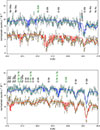 |
Fig. A.1. Continued. |
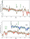 |
Fig. A.1. Continued. |
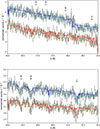 |
Fig. A.1. Continued. |
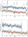 |
Fig. A.1. Continued. |
External absorption originating in the Milky Way may display the same lines as those of WA, which may provide additional complication in the analysis of the intrinsic absorption by the ionized gas at the source rest frame. In order to determine which lines originate externally to the source, we perform an exercise by fitting multiphase Galactic absorption with a more advanced model. The term responsible for the Galactic absorption in the cold phase was fit by the Ismabs model (Gatuzz et al. 2015), while the warm and hot Galactic phases (Nicastro et al. 2016; Gatuzz et al. 2016) were modeled through the models Ismabs and Ioneq (Gatuzz & Churazov 2018), respectively. The fit values of the parameters for the continuum model responsible for Galactic absorption are given in Tabs. A.1 and A.2. The column density of neutral hydrogen for the cold/warm phase in the Ismabs model was fixed at 4.44 × 1020 cm−2 (Murphy et al. 1996). Table A.1 displays all three ion populations of this model, i.e. neutral, single, and double ionized species, but only detectable ions are listed. In the hot phase fit by the Ioneq model, we left the column density of the neutral hydrogen as a free parameter. Only detectable ions are listed in Table A.2. We also tested a three-component Ioneq model instead of the aforementioned combination of Ismabs and a single Ioneq, but this approach did not result in better fit quality.
ISMABS model parameters fitting cold Galactic absorption.
IONEQ model parameters fitting warm/hot Galactic absorption.
By fitting Ioneq and Ismabs models, we were able to identify several Galactic absorption lines in our data, which are taken into account while identifying WA lines in Sect. 6.1. All Galactic absorption lines that may influence our analysis were cross-checked with the papers by Kaastra et al. (2009, 2011), Detmers et al. (2011), Kaastra et al. (2018), and are listed in the Table A.3. These lines are marked with green labels in Figs. A.1 to A.1 that present the final fit of the CTP WA model.
In addition, care is taken to identify instrumental features that are potentially not included in the response matrix of the RGS instrument. The instrumental lines together with the references are listed in Table A.4. For clarity of the figures presented in the final fit of high-resolution RGS data, we did not mark instrumental lines in the main body of the paper.
Galactic absorption lines identified during ISMABS and IONEQ model fitting to the Mrk509 RGS 1 and RGS 2 data.
Instrumental lines not included in the response matrix of RGS.
All Tables
Galactic absorption lines identified during ISMABS and IONEQ model fitting to the Mrk509 RGS 1 and RGS 2 data.
All Figures
|
Fig. 1. Spectral energy distribution of Mrk 509 used as an input to the photoionization code TITAN marked as a solid black line. The red circles are the observational points reported by Kaastra et al. (2011) and normalized to the incident flux. |
| In the text | |
|
Fig. 2. Continuum model and Galactic absorption fit to Mrk 509 RGS spectrum. RGS 1 and RGS 2 spectra are plotted in orange and cyan. RGS 2 is arbitrarily shifted by 0.02 counts s−1 Å−1. The continuum model of Mrk 509 SED absorbed by the Milky Way is marked with continuous red and blue lines. The lower panel shows residuals against the best-fit model. The wavelengths are in the observed frame of reference. For the purpose of this plot the data are binned by five channels. |
| In the text | |
|
Fig. 3. Dependence of O VII profile on the turbulent velocities used in photoionization computations by the TITAN code for a given model. |
| In the text | |
|
Fig. 4. Warm absorber on top of continuum modified by Galactic absorption with Mrk 509 RGS data points. RGS 1 and RGS 2 spectra are plotted in orange and cyan. RGS 2 is arbitrarily shifted by 0.02 counts s−1 Å−1. The total model consisting of continuum together with a single CTP WA is plotted in red and blue. The wavelengths are in the observed frame of reference. The lower panel shows residua. For the purpose of this plot the data are binned by five channels. |
| In the text | |
|
Fig. 5. BXA contour plots for fit parameters of the total model to the Mrk 509 RGS 1 and RGS 2 spectra. The cross-normalization factor shows the difference between two RGS specra where normalization gives the position of the total model. Best fit log |
| In the text | |
|
Fig. 6. Ionization structure of the best-fit CTP model computed by TITAN and fit to the Mrk 509 RGS data. The upper panel shows the structure of ionization parameter ξ, the medium panel the temperature, T (S-curve), and the bottom panel the volume density, nH, all versus the dynamical ionization parameter, Ξ. The illuminated cloud surface is located on the right side of the panels. |
| In the text | |
|
Fig. 7. Best-fit parameters using spectral windows with warm500 multiplicative model. |
| In the text | |
|
Fig. 8. Spectrum in the wavelength range of 12.3–12.7 Å containing Ne X line. |
| In the text | |
|
Fig. A.1. Overall model fit to Mrk 509 RGS spectrum given in observed frame. RGS 1 and RGS 2 spectra are plotted in orange and cyan dots with arbitrary shift 0.02 counts s−1 Å−1, and errors marked by gray bars. The total model: continuum together with single CTP WA is plotted in red and blue. WA lines are identified with black text, while possible absorption lines on Milky Way - by green text. For instrumental lines, see Appendix A. |
| In the text | |
|
Fig. A.1. Continued. |
| In the text | |
|
Fig. A.1. Continued. |
| In the text | |
|
Fig. A.1. Continued. |
| In the text | |
|
Fig. A.1. Continued. |
| In the text | |
Current usage metrics show cumulative count of Article Views (full-text article views including HTML views, PDF and ePub downloads, according to the available data) and Abstracts Views on Vision4Press platform.
Data correspond to usage on the plateform after 2015. The current usage metrics is available 48-96 hours after online publication and is updated daily on week days.
Initial download of the metrics may take a while.