| Issue |
A&A
Volume 705, January 2026
|
|
|---|---|---|
| Article Number | A255 | |
| Number of page(s) | 14 | |
| Section | Extragalactic astronomy | |
| DOI | https://doi.org/10.1051/0004-6361/202555592 | |
| Published online | 23 January 2026 | |
The observed total star formation rate function up to z ∼ 6: Complementary UV and IR contributions and comparison with state-of-the-art galaxy formation models
1
Istituto Nazionale di Astrofisica (INAF) – Osservatorio di Astrofisica e Scienza dello Spazio (OAS) Via Gobetti 101 I-40129 Bologna, Italy
2
Université Paris-Saclay, Université Paris Cité, CEA, CNRS, AIM F-91191 Gif-sur-Yvette, France
3
INAF – Osservatorio Astronomico di Padova, Vicolo dell’Osservatorio 3 I-35122 Padova, Italy
4
INAF – Osservatorio Astrofisico di Arcetri Largo E. Fermi 5 50125 Firenze, Italy
5
INAF – Astronomical Observatory of Trieste Via G.B. Tiepolo 11 I-34143 Trieste, Italy
6
IFPU – Institute for Fundamental Physics of the Universe Via Beirut 2 34151 Trieste, Italy
7
Institute for Physics, Laboratory for Galaxy Evolution and Spectral Modelling, Ecole Polytechnique Federale de Lausanne, Observatoire de Sauverny Chemin Pegasi 51 CH-1290 Versoix, Switzerland
8
School of Physics and Astronomy, Sun Yat-sen University, Zhuhai Campus 2 Daxue Road Xiangzhou District Zhuhai, China
9
Tianjin Normal University Binshuixidao 393 Tianjin, China
10
Max Planck Institut für Astronomie Königstuhl 17 D-69117 Heidelberg, Germany
11
Purple Mountain Observatory, Chinese Academy of Sciences 10 Yuanhua Road Nanjing 210023, China
12
Argelander-Institut für Astronomie, Universität Bonn Auf dem Hügel 71 53121 Bonn, Germany
13
Institute of Astronomy and Astrophysics, Academia Sinica, 11F of Astronomy-Mathematics Building, No. 1, Section 4 Roosevelt Road Taipei 106216, Taiwan, R.O.C.
14
SISSA Via Bonomea 265 34136 Trieste, Italy
15
IRA-INAF Via Gobetti 101 40129 Bologna, Italy
16
Cosmic Dawn Center (DAWN), Denmark
17
DTU-Space, Technical University of Denmark Elektrovej 327 DK-2800 Kgs. Lyngby, Denmark
18
Dipartimento di Fisica e Astronomia (DIFA), Universití di Bologna via Gobetti 93/2 I-40129 Bologna, Italy
★ Corresponding author: This email address is being protected from spambots. You need JavaScript enabled to view it.
Received:
20
May
2025
Accepted:
12
November
2025
Abstract
Aims. We investigated how the obscured IR-derived and dust-corrected UV star formation rate functions (SFRFs) compare with each other and with predictions from state-of-the-art theoretical models of galaxy formation and evolution.
Methods. We derived the IR SFRF from the ALMA A3COSMOS survey by converting the IR luminosity functions (IR LFs) into SFRFs after correcting for the active galactic nucleus (AGN) contribution. Similarly, we obtained the UV SFRFs from UV LFs in the literature, corrected for dust-extinction. First, we fit the two SFRFs independently via a Markov chain Monte Carlo (MCMC) approach, then we combined them to obtain the first estimate of the “total” SFRF out to z ∼ 6. Finally, we compared this SFRF with predictions of a set of theoretical models.
Results. We derive the UV and IR SFRFs at 0.5 < z < 6, using dust-extinction-corrected UV LFs from the literature and IR LFs from Herschel and ALMA. We find that the two functions are largely complementary, covering different ranges in star formation rate (SFR < 10–100 M⊙yr−1 for the UV-corrected, and SFR > 100 M⊙yr−1 for the IR). From the comparison of the total SFRF with model predictions, we find overall good agreement at z < 2.5, with increasing difference at higher redshifts; all models miss the galaxies that form stars with the highest SFRs. Finally, we finally obtain the UV (dust-corrected), IR and total SFR densities (SFRDs), finding that there are no redshift ranges where UV and IR alone are able to reproduce the total SFRD.
Key words: surveys / galaxies: evolution / galaxies: formation / galaxies: high-redshift / galaxies: star formation / submillimeter: galaxies
© The Authors 2026
 Open Access article, published by EDP Sciences, under the terms of the Creative Commons Attribution License (https://creativecommons.org/licenses/by/4.0), which permits unrestricted use, distribution, and reproduction in any medium, provided the original work is properly cited.
This article is published in open access under the Subscribe to Open model. This email address is being protected from spambots. You need JavaScript enabled to view it. to support open access publication.
1. Introduction
Understanding how galaxies form and evolve through cosmic time has been a topic of interest in both observational and numerical astrophysics over the past decades. Characterizing all of the physical mechanisms behind galaxy evolution is not an easy task and requires a variety of different observation strategies, including photometric and spectroscopic methods. Numerical simulations and theoretical models are widely used tools for investigating the physics that governs galaxy formation and evolution (White & Frenk 1991; Kauffmann et al. 1993; Springel et al. 2001; Bower et al. 2006; Croton et al. 2006; Monaco et al. 2007; Somerville et al. 2008; Fontanot et al. 2009; Guo et al. 2011; Benson 2012; Menci et al. 2012; Somerville et al. 2012; Henriques et al. 2013; Gruppioni et al. 2015; Henriques et al. 2015; Schaye et al. 2015; Pillepich et al. 2018; Davé et al. 2019; Lacey et al. 2016; Lagos et al. 2018). Observational studies have shown that star-forming galaxies (SFGs) populate a relatively tight “main sequence” (MS), relating stellar mass and star formation rate (Noeske et al. 2007; Whitaker et al. 2012; Speagle et al. 2014). The small scatter of the MS suggests that galaxies grow in a quasi-equilibrium state, regulated by the balance between gas accretion, star formation, and outflows (Bouché et al. 2010; Lilly et al. 2013; Davé et al. 2012). In the ΛCDM framework, galaxies are fueled by cold gas inflows from the cosmic web (Kereš et al. 2005; Dekel et al. 2009), while stellar and AGN-driven Consider defining AGN.*** outflows regulate their efficiency at converting gas into stars (Hopkins et al. 2014; Somerville & Davé 2015; Naab & Ostriker 2017). Both processes are incorporated into theoretical models through sub-grid prescriptions in simulations or empirical recipes in semi-analytical models (SAMs), where they strongly shape the predicted star formation rate function (SFRF) (Dubois et al. 2016). Comparing UV and IR observations with such models is therefore crucial for assessing the fidelity of feedback and dust implementations (Picouet et al. 2023). To trace galaxy evolution, a key aspects is to investigate the assembly of mass and the timescale over which the gas is converted into newly formed stars. The SFR provides the most accurate indicator for retrieving information on the instantaneous growth in stellar mass (M★).
Although the SFR of galaxies is an informative parameter for investigating galaxy evolution, its derivation is subject to several limitations, depending on the observed wavelengths. Different methodologies involve either detailed spectral energy distribution (SED) fitting or the use of star formation indicators. However, measurements derived from luminosities in different bands, such as the ultraviolet (UV) or infrared (IR), as well as individual nebular emission lines (e.g., Hα), can lead to diverging SFR estimates. Each of these galaxy luminosity probes has been calibrated in the local Universe to a corresponding SFR (e.g., Kennicutt 1998a,b; Kennicutt & Evans 2012; Smit et al. 2012), and it is unclear whether the same calibrations and assumptions, such as the initial mass function (IMF), can be applied at higher redshifts. In particular, UV and IR emission trace star formation on very similar timescales (see Kennicutt & Evans 2012). From a theoretical perspective, UV and IR luminosities of simulated galaxies are often derived by applying dust radiative transfer post-processing to the intrinsic stellar populations (e.g., Trayford et al. 2017; Narayanan et al. 2021). The SIMBA simulation represents an exception, as it includes a self-consistent dust production model (Davé et al. 2019), enabling direct predictions of both obscured and unobscured star formation. Picouet et al. (2023) show that the choice of feedback implementation and dust modeling critically affects the ability of models to reproduce the observed UV- and IR-derived SFRFs.
Observations in the optical and UV have enabled estimates of the star formation rate density (SFRD) up to redshifts of z ∼ 7 − 8 (see, e.g., Bouwens et al. 2014; Oesch et al. 2015; Laporte et al. 2016; Oesch et al. 2018), and even as high as z ∼ 10 (e.g., Harikane et al. 2023), significantly extending our understanding of star formation in the early Universe. However, these measurements–primarily based on rest-frame UV data–are likely missing the most dust-obscured, and thus star-forming, galaxies. In contrast, IR LFs are still poorly constrained beyond z ∼ 5, with the faint end in particular remaining largely unconstrained (although some attempts have been made to estimate it, e.g., Barrufet et al. 2023; Fujimoto et al. 2024).
Over the last fifteen years, many studies have investigated the main processes regulating star formation and have compared the observed SFRF (Reddy et al. 2008; Oesch et al. 2010; van der Burg et al. 2010; Ly et al. 2011; Magnelli et al. 2011; Cucciati et al. 2012; Smit et al. 2012; Gruppioni et al. 2013; Magnelli et al. 2013; Patel et al. 2013; Sobral et al. 2013; Duncan et al. 2014; Bouwens et al. 2015; Alavi et al. 2016; Parsa et al. 2016; Gruppioni et al. 2020) with predictions from simulations and models (Davé et al. 2011; Fontanot et al. 2012; Tescari et al. 2014; Gruppioni et al. 2015; Katsianis et al. 2017a, 2021b). These studies reveal tensions between observations and models, often linked to feedback implementations and dust treatments. While UV and IR estimates provide complementary information, models without adequately calibrated AGN or supernova (SN) feedback or dust prescriptions cannot simultaneously reproduce both the faint and bright ends of the SFRF (Gruppioni et al. 2015; Picouet et al. 2023).
To investigate the evolution of the SFR with redshift, and to alleviate the aforementioned tensions, large surveys are required. The automated mining of the ALMA archive in COSMOS (A3COSMOS, Liu et al. 2019; Liu & A3COSMOS Team 2019), which is the largest ALMA survey to date, represents an ideal benchmark for simulations and SAMs, probing the IR-mm SFRF over a wide redshift range (z ∼ 0 − 6). A physical and statistical analysis of the A3COSMOS galaxy sample has already been performed by Traina et al. (2024), hereafter T24, who aimed to derive the IR luminosity function (IR LF) and cosmic dust-obscured SFRD at different redshifts. From the same database, with the addition of the GOODS-S ALMA archival images, Adscheid et al. (2024) derive the (sub-)millimeter ((sub)-mm) number counts, while other physical properties (e.g., molecular gas and dust attenuation) are explored in previous works by Liu & A3COSMOS Team (2019), Fudamoto et al. (2020), Wang et al. (2022). In this paper, we use the IR LFs derived in T24 from the A3COSMOS survey, along with UV LFs from the literature, to obtain new estimates of the combined1 (IR and UV) SFRF at 0 < z < 6 and compare it with predictions from state-of-the-art hydrodynamical simulation and SAMs from the literature.
The paper is organized as follows: in Section 2, we present the archival samples used to derive the SFRFs; in Section 3 we derive the IR SFRF for the A3COSMOS survey, combine it with observational UV results, and compare it with fiducial models prediction of the SFRF from a set of hydrodynamical simulation and SAMs in Section 4; in Section 5, we compare the observed SFRD with the predicted values; in Section 6, we present the conclusions. Throughout the paper, we assume a Chabrier (2003) stellar IMF and adopt a ΛCDM cosmology with H0 = 70 km s−1 Mpc−1, Ωm = 0.3, and ΩΛ = 0.7.
2. The data
2.1. Infrared-millimeter (IR-mm) sample
The A3COSMOS survey is the largest database of ALMA-selected galaxies. It comprises all archival ALMA observations within the COSMOS field (Scoville et al. 2007; Weaver et al. 2022). In this study, we used the most recent version of the A3COSMOS combined with COSMOS2020 photometry (Weaver et al. 2022; Adscheid et al. 2024). We used the IR LF from T24, obtained by combining the A3COSMOS database (converted into a “blind-like” survey) with Herschel data points from Gruppioni et al. (2013). In the following, we summarize how the final A3COSMOS sample was obtained and its main physical properties. The T24 sample was obtained as follows: for each ALMA pointing, we removed sources within a radius of 1″ from the center (identified as targets of the ALMA observations) to avoid selection bias, as well as offset sources at a redshift similar to that of the target to correct for clustering bias. The final sample consists of 189 galaxies (out of an initial sample of 1620) which are considered serendipitously detected in the ALMA pointings. The main integrated galaxy physical properties (i.e., stellar mass, dust luminosity, and IR-SFR) were inferred in T24 through SED fitting with the CIGALE SED fitting code (Boquien et al. 2019), revealing a massive (M★ ∼ 1010 − 1012 M⊙), infrared-luminous (LIR, 8 − 1000 ∼ 1011 − 1013 L⊙) and highly star-forming (SFR ∼10 − 1000 M⊙yr−1) population. Additionally, ∼40% of the sources host an AGN, with different AGN fractions (i.e., the fraction of AGN emission relative to the total IR emission in the 5–40 μm range from the CIGALE templates, fAGN, ranging from 0.3 to 0.8). Figure 1 shows the SFR distribution of the full 1620-galaxy sample (cyan histogram) and the subsample of 189 sources considered serendipitous detections in T24 (teal histogram). Both distributions peak at SFR ∼ 300 M⊙yr−1, but most objects were excluded from the parent A3COSMOS sample because they are targets.
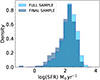 |
Fig. 1. Normalized density distributions of the IR-SFR obtained through SED fitting for the full A3COSMOS sample (cyan) and for the subsample used in this work (teal). |
2.2. UV datasets
Although star formation derived using the infrared luminosity (LIR) has been proven to account for a large fraction of the total SFR of a galaxy (Wuyts et al. 2011; Pannella et al. 2015), it traces only the obscured part and the fractional IR contribution to UV-derived SFRs may change at z > 3. For this reason, we included in our analysis the UV LFs from seven literature studies, broadly spanning the redshift range 0–6 (consistent with our IR-mm sample):
-
van der Burg et al. (2010) derived the UV LF in the range 3 < z < 5, using ∼105 Lyman-break galaxies from the CFHT Legacy Survey Deep fields.
-
Cucciati et al. (2012) studied the UV LF of I-band-selected galaxies using the VVDS surveys, from the local Universe up to z ∼ 4.5.
-
Parsa et al. (2016) explore the UV LF from z ∼ 2 to z ∼ 4, combining the HUDF, CANDELS/GOODS-South and UltraVISTA/COSMOS surveys.
-
Mehta et al. (2017) use the UVUDF to derive the UV LF of Lyman-break galaxies at z ∼ 1.5 − 3.
-
Ono et al. (2018) study the UV LF towards higher redshifts (z ∼ 4 − 7) through the Great Optically Luminous Dropout Research Using Subaru HSC (GOLDRUSH).
-
Adams et al. (2020) derive the LF at z ∼ 4, combining the COSMOS survey and the XMM-Newton Large-Scale Structure fields.
-
Bouwens et al. (2021, 2022) use a combination of several fields to derive the UV LF at z ∼ 2 − 9.
Using these data, we account for the unobscured contribution to the total SFRF at each redshift.
3. The IR and UV SFR function
To derive the SFRFs, we began with the IR and UV luminosity functions, converting LIR and UV magnitudes into IR-SFR and UV-SFR, respectively. Specifically, for the conversion of LIR to IR-SFR (which accounts for the obscured part of the SFR), we employed the following Kennicutt (1998a) relation (for a Chabrier IMF):
 (1)
(1)
To derive the component of the SFR from the UV luminosity, corrected for dust attenuation, we applied the following procedure. We corrected UV magnitudes in a self-similar manner via the same relation proposed by (Hao et al. 2011):
 (2)
(2)
where τUV represents the effective optical depth (τUV = A1600/1.086, with A1600 being the dust absorption at 1600 Å, calculated as A1600 = 4.43 + 1.99β). We adopted the form for β as shown in Bouwens et al. (2012):
 (3)
(3)
with MAB being the absolute UV magnitude. For  , we adopted the values tabulated by Tacchella et al. (2013) for various redshift intervals.
To derive the SFR from the UV luminosity, we used the corrected UV LF estimates for dust attenuation (see Section 3.2 for details), converting the absolute UV magnitude (for the catalogs described in Section 2.2) into UV luminosity as
 (4)
(4)
Finally, from LUV, corr, we then calculated the UV corrected component of the SFR as follows (see Kennicutt & Evans 2012):
 (5)
(5)
We computed the IR and UV SFRFs at z ∼ 0.5 − 6, dividing the z range into eight redshift bins similar to those explored by the UV and IR studies used in this work. The UV and IR SFRF data points are shown in Figure 2 (upper panel). Overall, there is reasonable agreement between the UV and IR data points. In particular, at 0 < z < 1.5, the points from both tracers nearly overlap in the range where data are available, with IR reaching higher SFR values and UV showing slightly lower ones. At higher redshifts, the bright end of the UV SFRF begins to deviate from that of the IR SFRF, which decreases less drastically. This discrepancy may be attributed to the difficulty for UV observations to detect the most dust-obscured galaxies with the highest SFRs (e.g., SFR > 103 M⊙ yr−1). Conversely, at higher redshifts, IR-mm observations become less sensitive to galaxies in low star-forming regimes. At the lowest redshift bins, UV and IR data points cover approximately the same SFR range, whereas at higher redshifts, UV data cover a wider range, especially at the faint end, but do not reach high SFR values that IR data do.
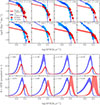 |
Fig. 2. Upper panel: UV and IR SFRFs at different redshifts. Data points are plotted in cyan (UV) and red (IR), with best-fit curves shown as blue (UV) and red (IR). Lower panel: Product of volume density (Φ) and SFR in each redshift bin, which is integrated to obtain the SFRD. The UV (blue area) and the IR (red area) SFR density distributions are compared at different redshifts as a function of the SFR. Both curves are normalized so that the UV peak is at 1. |
As a result, the UV dust-corrected and IR SFR functions may display different shapes while yielding similar integrated SFRD. We discuss these aspects in more detail in the following section.
3.1. Star formation rate function (SFRF) fitting procedure
To measure the IR SFRFs (from A3COSMOS) and UV SFRFs (from the studies listed in Section 2.2), we first fit the data points for IR and UV separately by performing a Markov chain Monte Carlo (MCMC) analysis. This procedure provided the best-fit IR and UV SFRFs across several redshift bins. We performed the MCMC using the PYTHON package emcee (Foreman-Mackey et al. 2013), which allowed us to explore the parameter space simultaneously using a set of walkers. Although UV SFRFs can be fitted with a classical Schechter function (Schechter 1976), IR SFRFs typically exhibit an excess at the bright end, which cannot adequately be modeled with a Schechter function (Lawrence et al. 1986; Soifer et al. 1987; Saunders et al. 1990; Rush et al. 1993; Shupe et al. 1998; Sanders et al. 2003). We therefore adopted a modified Schechter function (Saunders et al. 1990) for the IR SFRF fit. The classical Schechter function is characterized by three free parameters: the knee star formation rate (SFR*), the corresponding density of the galaxy population (Φ*), and the slope of the faint end (α). The modified Schechter function includes a fourth parameter, σ, which describes the shape of the bright end. The Schechter function is described by the following form:
![Mathematical equation: $$ \begin{aligned} \Phi (L)\mathrm{d}\log L = \Phi ^*\left(\frac{L}{L^*}\right)^{\alpha } exp\left[-\frac{L}{L^*}\right]\mathrm{d}\log L . \end{aligned} $$](/articles/aa/full_html/2026/01/aa55592-25/aa55592-25-eq7.gif) (6)
(6)
The modified Schechter can be written as
![Mathematical equation: $$ \begin{aligned} \Phi (L)\mathrm{d}\log L = \Phi ^*\left(\frac{L}{L^*}\right)^{1-\alpha _S} exp\left[-\frac{1}{2\sigma _S^2}\log _{10}^2 \left(1+\frac{L}{L^*}\right)\right]\mathrm{d}\log L. \end{aligned} $$](/articles/aa/full_html/2026/01/aa55592-25/aa55592-25-eq8.gif) (7)
(7)
Previous studies (e.g., Caputi et al. 2007; Béthermin et al. 2011; Gruppioni et al. 2013) have shown that these parameters, in particular L* and Φ*, evolve with redshift. In the IR domain, L* (a proxy for the dust-obscured SFR) increases with redshift, while Φ* of the galaxy population decreases (e.g., Gruppioni et al. 2013; Magnelli et al. 2013). This evolution can be described using a functional form that assumes a zbreak for both parameters, characterizing the change in their evolution with redshift. We adopted a similar redshift evolution for the UV SFRF, incorporating an evolving faint end slope, following Parsa et al. (2016). The equations describing the IR- and UV SFRF evolutions are
 (8)
(8)
 (9)
(9)
where Φ0* and SFR0* represent the normalization and characteristic SFR at z = 0, while kρ1, kρ2, kL1, and kL2 are the exponents of values below and above zρ0 and zL0 for Φ* and SFR*, respectively. The evolution of α in the UV (dust-corrected) SFRF fit is parametrized by the following power law:
 (10)
(10)
By exploiting the wide redshift range and the large number of independent datasets considered in this analysis, we constrained the best-fit parameters, identifying the local Schechter function and its evolution. Then, using the functional forms for the evolution presented above, we obtained the best-fit IR and UV SFRFs for each redshift bin. This approach allowed us to combine SFRF data from different studies at different redshifts within the same bands and after applying completeness corrections. To accurately constrain the parameters of the best-fit SFRFs, we also combined the A3COSMOS IR SFRFs with those obtained from Herschel PEP/HerMES surveys in the COSMOS, ECDFS, GOODS-N, and GOODS-S fields (Gruppioni et al. 2015). These surveys contain a much larger number of sources, particularly at low redshift, where ALMA provides limited statistics, as also done by T24 for the IR LFs.
The evolutive IR and UV SFRF best fits are shown in Figure 2 (upper panel). Because the fit was not performed individually for the data points in each redshift bin, some deviations between the data and the model at specific redshift bins may occur. We obtained the UV and IR SFRF best fits by simultaneously considering all data points across all redshifts and determining a redshift evolution compatible with the entire dataset. As noted above, there is a discrepancy of 0.5 to 1 dex in the SFR between the IR SFRF and the UV dust-corrected SFRF, which confirms that different indicators yield different results (Leja et al. 2020; Katsianis et al. 2020; Das & Pandey 2024). Most of this difference arises from the distinct SFR ranges traced by the two datasets and from differing slopes at the faint and bright ends of both SFRF best fits. This issue is illustrated in Figure 2 (lower panel), where we show the SFR density distribution integrated to obtain the SFRD (i.e., Φ* × SFR). Up to z ∼ 3, the UV integral exceeds the IR contribution, while at z > 3 the IR contribution increases rapidly. However, at all redshifts, the two functions span different SFR intervals. This implies that the same value of the cosmic SFRD could be obtained by two completely different distributions and, consequently, that neither the IR nor the UV alone can account for the total SFRD at any given redshift. In the next section, we address this issue by defining a total IR & UV SFRF, whose evolution is studied in Section 5.
3.2. The IR + UV total SFRF
To compare our results with predictions from simulations and SAMs, which predict the total SFRF, we must derive the same quantity from data (i.e., a total SFRF). As discussed in the previous section, neither the IR SFRF nor the dust-corrected UV SFRF can represent the total SFRF because, even after completeness and dust corrections, neither can sample the whole range of SFRs. We therefore needed to derive the best representation of the total SFRF, covering all relevant SFR values. To this end, we combined the UV and IR SFRF data and performed an MCMC fit under the following assumptions. In principle, to derive the total SFRF, we should use the same galaxy sample and sum the obscured (IR-traced) and unobscured (UV-traced and uncorrected for dust extinction) SFRs for each galaxy. However, as shown by Figure 2, no galaxy samples have IR and UV observations that cover identical SFR intervals, although some partially overlap. Surveys in the UV typically sample fainter SFR but are not able to detect the most star-forming (and obscured) systems, whereas IR surveys are sensitive to the higher SFRs but are not deep enough to detect fainter SFR galaxies, containing small amounts of dust. Given the complementarity of the two SFRFs traced by UV and IR (Figure 2), we assume that the faint end of the UV FRF (corrected for dust attenuation) traces ∼100% of the SFR at low SFRs, and that the bright end of the combined SFRF is almost entirely traced by the highest-SFR galaxies. Under these assumptions, we fit a single functional form to the UV SFRF data at SFR < SFRUV* and to the observed IR SFRF data at SFRs above the IR completeness threshold. The global fit to the data represents the best estimation of the total SFRF.
Before proceeding, to verify whether our assumptions are reasonable and valid in a wide redshift range, we performed a simple test to derive the combined SFRF by assuming a certain stellar mass function (SMF) and galaxy main sequence (MS), which we then compared with the total SFRF from all data. Details of this test are provided in Appendix A, and the result, which confirms the robustness of our method, is shown in Figure A.1.
A similar approach was adopted by Mancuso et al. (2016a,b), who simultaneously fit the IR and UV (dust-corrected) SFRFs with a Schechter function, using all IR and UV data points up to 30 M⊙ yr−1. Their results clearly show that the UV and IR trace different SFR regimes and are therefore both required to compute the total SFRF. Similar findings were reported by Bernhard et al. (2014), Rodríguez-Puebla et al. (2020), showing that the IR and UV bands trace distinct and largely complementary regimes of galaxy types in terms of stellar masses and SFRs, with the IR tracing typically the most massive, star-forming galaxies, while the UV traces the faintest ones.
To perform the combined UV and IR SFRF, we fit the data in each individual z-bin using a modified Schechter, without fixing the faint- and bright-end slopes. Specifically, we left αS, σS (the slope parameters), Φ*, and L* free to vary in each bin (see Table 1). Unlike previous fits, we chose to fit the data points in each redshift bin individually, as there is no clear evidence in the literature for evolution for a “total” SFRF. Figure 3 shows the results of the combined SFRF fit. In most bins, the modified Schechter function provides a good fit to the data in both the UV and IR regimes, allowing us to characterize the properties of the SFRF simultaneously across the faint and bright ends as well as in the knee. We note that at z > 2, this parametrization of the SFRF lacks reliable or complete data over part of the SFRF range. Although this has limited impact, it may influence the final fit because it covers the range of the SFRF knee. Figure 3 also compares our results with those of Mancuso et al. (2016b) and Picouet et al. (2023), who applied similar approaches to estimate the total SFRF. Specifically, Mancuso et al. (2016b) combine UV and IR LF data to cover both the faint and bright ends of the SFRF, while Picouet et al. (2023) use FIR data from the COSMOS2020 catalog and U-band observation from the HSC-CLAUDS survey. Our results are consistent with both studies, with comparability up to z ∼ 3.
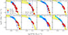 |
Fig. 3. Combined SFRF best-fit. The UV and IR data points are the same as in Figure 2. Open blue circles indicate the UV points excluded from the combined fit. The combined best-fit is shown as a yellow shaded region, corresponding to the 16th and 84th percentiles from the MCMC analysis. |
Best-fit parameters of the total UV and IR SFRFs.
4. Comparison with hydrodynamical simulations and semi-analytical models
We compared our total IR & UV SFRF results with predictions from state-of-the-art simulations and semi-analytical models. Specifically, we compared with the SFRF from the EAGLE simulation (Schaye et al. 2015; Crain et al. 2015) by Katsianis et al. (2017a), IllustrisTNG (Pillepich et al. 2018), and SIMBA (Davé et al. 2019) hydrodynamical simulations, the GAlaxy Evolution and Assembly (GAEA) code (Hirschmann et al. 2016; Fontanot et al. 2020), and L-GALAXIES SAMs (Henriques et al. 2020; Parente et al. 2023). Below, we briefly describe these theoretical frameworks; the main features of each model are summarized in Tables B.1 and B.2 of Appendix B. Figure 4 shows the predicted SFRFs alongside our estimates.
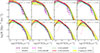 |
Fig. 4. Observed SFRF compared with predictions from simulations and SAMs. The yellow region represents the observed data used for the fit. The black curve indicates the best fit. The dashed purple line represents the SFRF from the EAGLE simulation, the dashed pink curve shows the result from the SIMBA simulation, and the magenta line corresponds to IllustrisTNG (Katsianis et al. 2017a, 2021a). The lime-green and green dotted curves show the predictions from the GAEA SAM by Hirschmann et al. (2016) and Fontanot et al. (2020), respectively. Finally, the dotted cyan curves show the predictions by Parente et al. (2023). |
4.1. Hydrodynamical simulations
Hydrodynamical simulations aim to follow galaxy formation in a direct and self-consistent manner by numerically solving the coupled evolution of dark matter and baryonic matter. They incorporate gravitational dynamics, gas hydrodynamics, and sub-grid models for unresolved processes such as star formation and feedback, enabling a detailed characterization of the physical mechanisms that regulate star formation. However, their high computational cost typically limits the accessible cosmological volume, which can impact the statistical sampling of rare objects relevant to the high-SFR end of the SFRF.
4.1.1. EAGLE
In the context of stellar formation, the EAGLE simulation incorporates the methodology proposed by Dalla Vecchia & Schaye (2008), in which the gaseous medium is categorized into distinct phases: cold molecular clouds, warm atomic gas, and ionized hot gas bubbles. The star formation rate is estimated using the Kennicutt-Schmidt relation (Schmidt 1959), derived from the surface density of both stars and gas. The simulation includes supermassive black holes (SMBHs), with seeds placed at the center of massive dark matter (DM) halos. The feedback from AGNs is assumed to be responsible for the quenching of massive galaxies and is tuned to reproduce the high-mass end of the galaxy stellar mass function (GSMF) at z = 0. In this work, we used the prediction corresponding to a cosmological box of size ∼100 Mpc. Figure 4 shows the predictions of the EAGLE simulation (dashed magenta curve). The SFR range covered by the predicted SFRF spans between 0.01 < SFR[M⊙ yr−1] < 2, allowing comparison with our results from the faint end and the knee of the SFRFs. At lower redshifts, the prediction reproduces the faint end of the combined SFRFs, while at z > 2.5, it reproduces the knee of the distribution with greater accuracy. The observed UV SFRFs agree well with the predictions from EAGLE Katsianis et al. (2017a) at these redshifts. In our work, we confirm the tension with the higher star formations probed by the IR observations. This discrepancy could be alleviated by decreasing the efficiency of the AGN feedback prescription (Katsianis et al. 2017a,b). It remains uncertain whether a larger box-size simulation with better statistics for the high star-forming galaxies would reproduce the observations without further re-tuning of the feedback prescriptions.
4.1.2. IllustrisTNG
The IllustrisTNG simulation (Pillepich et al. 2018, with a box size of ∼110 Mpc) is an improvement of the cosmological Illustris simulation (Genel et al. 2014; Vogelsberger et al. 2014), based on the AREPO (Springel 2010) code. Notable enhancements in IllustrisTNG include improvements to the prescriptions for supernova and AGN feedback. Galactic winds are injected isotropically, with increased wind factors in terms of velocity and energy, resulting in a more efficient overall quenching process in IllustrisTNG compared to its predecessor. For high BH accretion rates relative to the Eddington limit, the model assumes that a fraction of the accreted rest-mass energy thermally heats the surrounding gas. For low accretion rates, the simulation employs a purely kinetic feedback component, which imparts momentum to the surrounding gas in a stochastic manner. Unlike Illustris or EAGLE, the IllustrisTNG model was constrained to reproduce the observed cosmic star formation rate density (CSFRD) at z ∼ 0 − 10, so good agreement with the SFRF is not guaranteed but somewhat expected. The IllustrisTNG SFRF estimates can reach values up to log(SFR)∼3, allowing comparison with the high star-forming regime of the SFRF. The comparison is similar to that of the EAGLE simulation, with the IllustrisTNG SFRF showing slightly higher values of Φ at SFR > SFR*. Notably, at z > 3, where other cosmological models struggle to reproduce the knee of the combined SFRF, IllustrisTNG reproduces the observed SFRF reasonably well up to SFR ∼ 5 × 10² at z ∼ 5. Similarly to EAGLE, IllustrisTNG suffers from resolution effects, and the resulting SFRFs are also impacted by resolution (Zhao et al. 2020). If the model is run at lower or higher resolution, re-tuning of the feedback prescriptions is required to reproduce the observations (CSFRD and SFRF). In addition, a 100 Mpc box size is relatively small, so the simulation may not probe rare high star-forming objects.
4.1.3. SIMBA
The SIMBA simulation (Davé et al. 2019, box size ∼150 Mpc) is the upgraded version of the MUFASA (Davé et al. 2017), based on the GIZMO code (Hopkins 2015). The main enhancement is the inclusion of BH seeding and evolution, which plays a role in the quenching. Black hole (BH) accretion occurs through two channels: one sourced from cold gas and the other from hot gas. These fuel feedback mechanisms that suppress galaxy activity through kinetic bipolar outflows and X-ray heating. Unlike EAGLE or IllustrisTNG, SIMBA reproduces a bimodal specific SFRF (Katsianis et al. 2021a). This suggests that the sophisticated AGN feedback prescription is successful in reproducing observables related to galaxy stellar masses and SFRs. As observed for the previous two simulations, SIMBA reproduces the combined SFRF well at z < 2 − 2.5, but misses the most star-forming population and shows limitations at the low star-forming regime due to its lower resolution.
4.2. Semi-analytical models
Semi-analytical models (SAMs) provide an efficient and flexible framework for exploring galaxy formation and evolution. They are built upon dark matter halo merger trees, typically extracted from large N-body simulations, onto which simplified, physically motivated prescriptions for gas cooling, star formation, feedback, and chemical enrichment are applied. This approach allows SAMs to cover wide cosmological volumes and rapidly test the impact of different physical assumptions, making them particularly valuable for statistical comparisons with observed galaxy populations, such as the SFRF.
4.2.1. GAEA2016H, GAEA2020F, and GAEA2024M
We also compared our SFRF results with predictions from semi-analytic models. Specifically, we employed the predictions from the GAEA code, both in its standard version Hirschmann et al. (2016), hereafter GAEA2016H) and its updated version Fontanot et al. (2020), GAEA2020F) which corresponds to the F06-GAEA run in that paper. Both predictions are based on the Millennium simulation with a volume ∼5003 Mpc3. Both models describe baryonic evolution in four compartments: the stellar component of galaxies, cold gas within the galactic disk, hot gas in the dark matter halo, and the ejected gas component. This model was calibrated to reproduce the galaxy stellar mass function up to z ∼ 3, but it also provides good agreement with higher-redshift observations (Fontanot et al. 2017). In a more recent version of the model (Fontanot et al. 2020), the modeling of cold gas accretion onto SMBHs has been improved and better characterized, taking into account several triggering mechanisms (such as mergers and disk instabilities) for the loss of angular momentum of cold gas, leading to the formation of a reservoir from which material can be accreted onto the central BH. Finally, AGN feedback is also included in the form of AGN-driven outflows. A new version of the GAEA simulation, GAEA2024M (De Lucia et al. 2024), includes improvements in gas accretion onto SMBHs and gas interactions involved in the stripping of satellite galaxies.
All three GAEA versions (GAEA2016H, GAEA2020F, and GAEA2024M) agree well with our data points and best fits in most redshift bins. At higher redshifts, the models diverge from the data, particularly at the highest star-forming end, though the results remain consistent within fit uncertainties.
4.2.2. L-GalP23
The L-GALAXIES SAM (Henriques et al. 2020) is the latest public release of the Munich galaxy formation model. It runs on top of the Millennium simulation (Springel 2005) and models the evolution of both the stellar and gaseous components of DM halos by taking into account a number of astrophysical processes, including feedback from SNe and AGNs (in the radio mode). Here, we compare our results with the predictions from the L-GALAXIES model, incorporating updates introduced in Parente et al. (2023) and hereafter referred to as the L-GalP23 version. These updates include a detailed treatment of dust evolution and a novel prescription for disk instabilities, which considers the instability of both stellar and gaseous disks. The gaseous disk, in particular, can induce starbursts and accrete the central SMBH. Similarly to other models, the L-GalP23 predictions largely reproduce the faint end of the SFRF.
The comparison between our results and the simulations described above shows that, although most models have difficulties reproducing the bright end of the SFRF at z > 2, some progress had been made in characterizing the physical processes that regulate star formation in galaxies. Indeed, the agreement between data and models has improved significantly compared to similar studies from previous years (e.g., Gruppioni et al. 2015), now achieving good agreement with data up to z ∼ 3.5 − 4. However, all models considered here predict lower SFRF values at SFR > 103 M⊙ yr−1. As noted by (Katsianis et al. 2021b), IR SFRFs at these regimes are overestimated due to: (i) dust being heated by old populations unrelated to current star formation; (ii) larger polycyclic aromatic hydrocarbon emission in distant galaxies; (iii) ultra-luminous IR galaxies at high redshift being offset from the typically used SFR calibration adopted by Kennicutt (1998a; iv) neglect of the Eddington bias at the high star-forming end; and (v) residual AGN activity in the most IR-luminous sources. However, these effects should contribute only a negligible fraction of the IR luminosity. In particular, effects such as the Eddington bias (which may affects the bright-end of the SFRF, see e.g., Ilbert et al. 2013; Picouet et al. 2023) may represent a subdominant source of uncertainties (∼0.1 dex, see e.g., Caputi et al. 2011). This is especially true in our case, where the uncertainties on the SFRF fit are dominated by the errors on the photometric redshifts of the sample and the errors on the IR luminosities. We accounted for these uncertainties by performing a bootstrap resampling of the SFRs within their errors. An additional source of discrepancy is the effect of metallicity on the conversions typically used in the literature (and also in this work) to obtain the SFR from a luminosity. Indeed, several studies Madau & Dickinson (2014), Tacchella et al. (2018), Rodríguez-Puebla et al. (2020) have shown that neglecting metallicity can cause errors up to ∼0.5 dex. For comparison purposes, we used standard calibration factors. Finally, cosmic variance has been shown to be negligible in surveys composed of several pointings driver?robotham2010MNRAS.407.2131D. Specifically, Adscheid et al. (2024) show that the effect of cosmic variance on A3COSMOS is negligible.
5. The total SFRD
In this section, we present the cosmic SFRD from the integration of the combined SFRFs and compare SFRDTOT with the estimates obtained by integrating the predictions of the simulations and SAMs.
5.1. Total SFRD
To compute the total SFRD, we integrated the total SFRF down to SFR = 0.03 × SFR*, following the approach of Madau & Dickinson (2014). We then investigated what fraction of the total SFRD can be estimated by either the IR or the UV (dust-corrected) SFRDs. This comparison is shown in Figure 5. We emphasize that, in this comparison, the UV and IR SFRD do not sum to unity, as the figure shows the fraction of the total SFRD recovered when the IR or the UV probe was used individually. The UV dust-corrected SFRD, obtained by integrating the UV SFRF, recovers most of the total SFRD at z ∼ 1, but the ratio between the UV and total SFRD decreases at higher redshifts, becoming comparable with the IR estimates. The IR SFRD probes approximately 50% of the SFRD at z ∼ 1, and its contribution increases to ∼60% at z ∼ 5. Dust corrections are crucial at lower redshifts, where the observed UV SFRD is minimal, but become less important at higher redshifts, where the observed UV is compatible with the IR SFRD. Thus, the combination of UV and IR is fundamental to recover 100% of the SFRD for z ≳ 1.
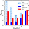 |
Fig. 5. Fraction of the combined SFRD recovered by UV (light blue and blue histograms) and IR (red histograms) data as a function of redshift. The filled blue histograms show the fraction recovered by the observed UV (i.e., without dust correction), while the light-blue dashed histograms correspond to the dust-corrected UV. We note that the UV and IR fractions do not sum to unity, since each SFRD is obtained by integrating the respective best-fit SFR function. |
The total SFRD obtained by integrating our total SFRF is presented in Figure 6. The upper panel compares it with the UV and IR results in the literature. Up to z ∼ 1.5, where the UV and IR SFRFs are still similar, our result agrees with most UV and IR estimates. From z ∼ 2 to z ∼ 4, the total SFRD is approximately twice as high as previous estimates based solely on IR or UV data, while at z ≳ 4.5 it remains broadly consistent with several UV-only and IR-only derivations.
5.2. Comparison with models
Similarly to the SFRF, we compared the total SFRD with the SFRD predictions from the models considered here (Figure 6, bottom panel). As expected, the EAGLE SFRD (purple line) cannot reproduce the observed SFRD in the covered SFR range because it does not extend to values greater than ∼100 M⊙ yr−1. This limitation was noted by Furlong et al. (2015). The SFRD from the SIMBA simulation (pink curve) shows a trend similar to that of EAGLE, remaining lower than the combined SFRD. The IllustrisTNG simulation (dashed magenta line, whose subgrid parameters were tuned to reproduce the observed CSFRD) reproduces the SFRD at high redshift (z > 3), while the GAEA SFRDs are consistent with our results up to z ∼ 1.5 but lower at higher redshifts, predicting an SFRD higher than that derived by Madau & Dickinson (2014). At z ∼ 4 − 5, GAEA is again consistent with our result. Finally, the modified version of the L-GalP23 models by Parente et al. (2023) produces an SFRD similar to those obtained using the EAGLE and SIMBA simulations. At low redshifts (z < 1), SAMs predict a higher SFRD than observed. This discrepancy may be attributed to an overproduction of star-forming galaxies in the local universe by SAMs (see e.g., Collacchioni et al. 2018). Conversely, at high redshifts (z > 2.5), there appears to be a deficiency in the fraction of galaxies exhibiting particularly active star formation (e.g., SFR > 1000 M⊙ yr−1), which characterizes the observed bright end of the IR SFRF.Gruppioni et al. (2015) show that a list of SAMs (e.g., Monaco et al. 2007; Henriques et al. 2015; De Lucia & Blaizot 2007) reproduce the bright end only up to z < 1 − 1.5, while the recent models by Hirschmann et al. (2016), Fontanot et al. (2020) and De Lucia et al. (2024) now match observations up to z ∼ 2 − 2.5. This demonstrates the improvement in SAMs over the last ten years.
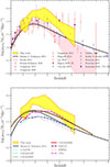 |
Fig. 6. Upper panel: SFRD obtained by integrating the combined SFRFs in each redshift bin (yellow area), compared to IR and UV results from the literature (shown as red and blue open symbols, respectively). Lower panel: SFRD compared with predictions from the models discussed in this work. The color code for the models is the same as in Figure 4. |
5.3. Fitting the cosmic SFRD
In this section, we provide a new fit to the observed total SFRD, adopting the same parametrization described in Madau & Dickinson (2014) (although Gamma functions or log-normal parametrizations may be more physically motivated; see e.g., Gladders et al. 2013; Katsianis et al. 2023). Madau & Dickinson (2014) fit the observed UV and IR SFRD with the following functional form:
![Mathematical equation: $$ \begin{aligned} \psi (z) = a \frac{(1+z)^\alpha }{1+[(1+z)/(1+z_{\rm peak})]^{\beta }} \,\, \text{ M}_{\odot }\,\text{ yr}^{-1} \text{ Mpc}^{-3}, \end{aligned} $$](/articles/aa/full_html/2026/01/aa55592-25/aa55592-25-eq44.gif) (11)
(11)
where a is the normalization at z = 0, zpeak is the redshift of the peak, α is the slope of the SFRD at z < zpeak, and β regulates the slope at z > zpeak. We fit the total IR and UV SFRD using an MCMC fitting procedure, leaving the four parameters free to vary. The result is shown in Figure 7. We obtain a slightly lower normalization than that found by Madau & Dickinson (2014) ( , aMD14 = 0.015); the slopes also differ, with
  (αMD14 = 2.7) and
  (βMD14 = 5.6). The main difference is a more pronounced peak at higher redshift:
  (versus zpeak, MD14 = 1.9). This may reflect more accurate IR measurements available today, which allow probing dust-obscured star formation up to higher redshifts (e.g., Algera et al. 2023; Liu et al. 2025; Sun et al. 2025).
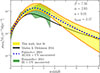 |
Fig. 7. Fit to the total SFRD using the functional form by Madau & Dickinson (2014). The best fit to our data is shown as the dashed orange line with yellow error bands. The Madau & Dickinson (2014) fit is plotted in black. A similar fit from Fujimoto et al. (2024) is shown as the dotted blue line, while the shaded green area represents the combined SFRD estimated by Burgarella et al. (2013). In the upper-right corner, we display the best-fit values of the free parameters of Equation (11). |
Our results agree with those of Burgarella et al. (2013), Fujimoto et al. (2024) who use a comprehensive IR + UV approach. The first study derives the LFs from the Herschel/PEP+HerMES surveys (FIR) (Gruppioni et al. 2013) and the UV using data from the VVDS (Cucciati et al. 2012). The authors compute the combined SFRD by adding the dust-obscured contribution (derived from the FIR) and the unobscured contribution (from the FUV) at 0 < z < 3.5 (covering the SFRD peak; Figure 7). They find that the SFRD rises between z ∼ 0 and z ∼ 1.5, then decreases gently to z ∼ 3.5. The total SFRD derived by Burgarella et al. (2013) has a higher normalization at the peak than Madau & Dickinson (2014), in agreement with our findings of a higher SFRD at 2 < z < 3. The second work, by Fujimoto et al. (2024), is obtained from the ALMA Lensing Cluster Survey, which covers a wide redshift range (1 < z < 8). Unlike Burgarella et al. (2013), they do not combine IR and UV LFs; however, due to the excellent sensitivity achieved by ALMA in a lensed field, they were able to probe lower values of the IR LF even at very high redshifts. By sampling the IR LF down to its faint end, they correctly estimated α, finding a steeper value than is typically fitted to the IR LF (see e.g., Gruppioni et al. 2013, 2020; Traina et al. 2024). Combining their dust-obscured SFRD with the unobscured SFRD from Bouwens et al. (2020), they derive the total SFRD over a very broad redshift range. Figure 7 shows our fit to their data using the same functional form. They find a normalization (a = 0.01) and redshift peak of the SFRD (zpeak ∼ 2.3), in very good agreement with our results. Fujimoto et al. (2024) report the SFRD estimates using two different lower limits for the integration of the IR LF. In particular, the fit in Figure 7 is obtained by integrating the IR LF down to LIR = 1010 L⊙, which is slightly higher than our lower integration limits (ranging from ∼4 × 10⁸ to ∼4 × 10⁹ L⊙). The authors also consider a less conservative integration limit, LIR = 108 L⊙, which leads to a higher estimate of the total SFRD (∼3× larger SFRD, see Figure 18 of their paper), which is even in better agreement with our results.
6. Summary and conclusions
By combining recent IR LF and SFRD from Traina et al. (2024) with dust-corrected UV SFRFs derived from the literature, we estimated the total (IR and UV) SFRF and SFRD in the redshift range z = 0.5 − 6. We also compared these results with predictions from state-of-the-art SAMs and hydrodynamical simulations to assess how well these models can reproduce observational estimates. The results can be summarized as follows:
-
The IR and UV dust-corrected star formation functions sample different ranges of SFRs. The UV SFRF extends to values below 10 M⊙ yr−1 up to z ∼ 2 and reaches values of 100 M⊙ yr−1 at higher redshifts. In contrast, the IR SFRF dominates at higher SFRs, particularly in the range 100–1000 M⊙ yr−1 (in agreement with previous works, e.g., Katsianis et al. 2017b, 2021b).
-
Using the dust-corrected UV SFRF data points at SFR values below the knee and the IR SFRF at values above the knee, we derive the total best-fitting SFRF. Comparison of the total SFRF with predictions from simulations and SAMs reveals that the latter are capable of reproducing the faint end well at all redshifts, but the bright end only up to z ∼ 2 − 2.5. At higher redshifts, the models lack galaxies with very high SFR, which are responsible for the bright end of the observed SFRF.
-
The total SFRD shows a typical increasing trend at 0.5 < z < 1.5, a broad peak up to z ∼ 3, and a decrease towards z ∼ 6. The models predict an SFRD consistent with observed values up to z ∼ 2. At higher redshifts, they are consistent within the errors. The ratios between IR and total SFRD and UV (dust-corrected) and total SFRD are useful to quantify the extent to which both tracers reproduce the evolution of total SFRD. Both tracers are able to reproduce it up to z ∼ 1, but at higher redshifts, they only account for ∼60% of the total SFRD.
-
We fit the total SFRD with the same functional form as adopted by Madau & Dickinson (2014) and Fujimoto et al. (2024). We find that the peak of the SFRD is located at higher redshifts (zpeak ∼ 2.6) and has a higher normalization compared with that obtained by Madau & Dickinson (2014). Our results are consistent with the observed total SFRD by Burgarella et al. (2013) and recent results by Fujimoto et al. (2024), who find very similar peak normalizations and redshifts.
Acknowledgments
AT acknowledges support from the “INAF Ricerca Fondamentale 2023 – Large GO” grant. AK is supported by the Guangdong Basic and applied Basic research foundation (No: 2025A1515012670) and the 100 talents program of Sun Yat-sen University. SA gratefully acknowledges the Collaborative Research Center 1601 (SFB 1601 sub-project C2) funded by the Deutsche Forschungsgemeinschaft (DFG, German Research Foundation) – 500700252. ID acknowledges funding by the European Union – NextGenerationEU, RRF M4C2 1.1, Project 2022JZJBHM: “AGN-sCAN: zooming-in on the AGN-galaxy connection since the cosmic noon” – CUP C53D23001120006.
References
- Adams, N. J., Bowler, R. A. A., Jarvis, M. J., et al. 2020, MNRAS, 494, 1771 [NASA ADS] [CrossRef] [Google Scholar]
- Adscheid, S., Magnelli, B., Liu, D., et al. 2024, A&A, 685, A1 [NASA ADS] [CrossRef] [EDP Sciences] [Google Scholar]
- Alavi, A., Siana, B., Richard, J., et al. 2016, ApJ, 832, 56 [Google Scholar]
- Algera, H. S. B., Inami, H., Oesch, P. A., et al. 2023, MNRAS, 518, 6142 [Google Scholar]
- Barrufet, L., Oesch, P. A., Bouwens, R., et al. 2023, MNRAS, 522, 3926 [NASA ADS] [CrossRef] [Google Scholar]
- Benson, A. J. 2012, New Astron., 17, 175 [NASA ADS] [CrossRef] [Google Scholar]
- Bernhard, E., Béthermin, M., Sargent, M., et al. 2014, MNRAS, 442, 509 [NASA ADS] [CrossRef] [Google Scholar]
- Béthermin, M., Dole, H., Lagache, G., Le Borgne, D., & Penin, A. 2011, A&A, 529, A4 [Google Scholar]
- Boquien, M., Burgarella, D., Roehlly, Y., et al. 2019, A&A, 622, A103 [NASA ADS] [CrossRef] [EDP Sciences] [Google Scholar]
- Bouché, N., Dekel, A., Genzel, R., et al. 2010, ApJ, 718, 1001 [Google Scholar]
- Bouwens, R. J., Illingworth, G. D., Oesch, P. A., et al. 2012, ApJ, 754, 83 [Google Scholar]
- Bouwens, R. J., Bradley, L., Zitrin, A., et al. 2014, ApJ, 795, 126 [Google Scholar]
- Bouwens, R. J., Illingworth, G. D., Oesch, P. A., et al. 2015, ApJ, 803, 34 [Google Scholar]
- Bouwens, R., González-López, J., Aravena, M., et al. 2020, ApJ, 902, 112 [NASA ADS] [CrossRef] [Google Scholar]
- Bouwens, R. J., Oesch, P. A., Stefanon, M., et al. 2021, AJ, 162, 47 [NASA ADS] [CrossRef] [Google Scholar]
- Bouwens, R. J., Illingworth, G., Ellis, R. S., Oesch, P., & Stefanon, M. 2022, ApJ, 940, 55 [NASA ADS] [CrossRef] [Google Scholar]
- Bower, R. G., Benson, A. J., Malbon, R., et al. 2006, MNRAS, 370, 645 [Google Scholar]
- Burgarella, D., Buat, V., Gruppioni, C., et al. 2013, A&A, 554, A70 [NASA ADS] [CrossRef] [EDP Sciences] [Google Scholar]
- Caputi, K. I., Lagache, G., Yan, L., et al. 2007, ApJ, 660, 97 [NASA ADS] [CrossRef] [Google Scholar]
- Caputi, K. I., Cirasuolo, M., Dunlop, J. S., et al. 2011, MNRAS, 413, 162 [NASA ADS] [CrossRef] [Google Scholar]
- Chabrier, G. 2003, PASP, 115, 763 [Google Scholar]
- Collacchioni, F., Cora, S. A., Lagos, C. D. P., & Vega-Martínez, C. A. 2018, MNRAS, 481, 954 [Google Scholar]
- Crain, R. A., Schaye, J., Bower, R. G., et al. 2015, MNRAS, 450, 1937 [NASA ADS] [CrossRef] [Google Scholar]
- Croton, D. J., Springel, V., White, S. D. M., et al. 2006, MNRAS, 365, 11 [Google Scholar]
- Cucciati, O., Tresse, L., Ilbert, O., et al. 2012, A&A, 539, A31 [NASA ADS] [CrossRef] [EDP Sciences] [Google Scholar]
- Dalla Vecchia, C., & Schaye, J. 2008, MNRAS, 387, 1431 [Google Scholar]
- Das, A., & Pandey, B. 2024, JCAP, 2024, 060 [Google Scholar]
- Davé, R., Oppenheimer, B. D., & Finlator, K. 2011, MNRAS, 415, 11 [Google Scholar]
- Davé, R., Finlator, K., & Oppenheimer, B. D. 2012, MNRAS, 421, 98 [Google Scholar]
- Davé, R., Rafieferantsoa, M. H., Thompson, R. J., & Hopkins, P. F. 2017, MNRAS, 467, 115 [NASA ADS] [Google Scholar]
- Davé, R., Anglés-Alcázar, D., Narayanan, D., et al. 2019, MNRAS, 486, 2827 [Google Scholar]
- De Lucia, G., & Blaizot, J. 2007, MNRAS, 375, 2 [Google Scholar]
- De Lucia, G., Fontanot, F., Xie, L., & Hirschmann, M. 2024, A&A, 687, A68 [NASA ADS] [CrossRef] [EDP Sciences] [Google Scholar]
- Dekel, A., Birnboim, Y., Engel, G., et al. 2009, Nature, 457, 451 [Google Scholar]
- Driver, S. P., & Robotham, A. S. G. 2010, MNRAS, 407, 2131 [Google Scholar]
- Dubois, Y., Peirani, S., Pichon, C., et al. 2016, MNRAS, 463, 3948 [Google Scholar]
- Duncan, K., Conselice, C. J., Mortlock, A., et al. 2014, MNRAS, 444, 2960 [Google Scholar]
- Fontanot, F., De Lucia, G., Monaco, P., Somerville, R. S., & Santini, P. 2009, MNRAS, 397, 1776 [NASA ADS] [CrossRef] [Google Scholar]
- Fontanot, F., Springel, V., Angulo, R. E., & Henriques, B. 2012, MNRAS, 426, 2335 [Google Scholar]
- Fontanot, F., Hirschmann, M., & De Lucia, G. 2017, ApJ, 842, L14 [Google Scholar]
- Fontanot, F., De Lucia, G., Hirschmann, M., et al. 2020, MNRAS, 496, 3943 [CrossRef] [Google Scholar]
- Foreman-Mackey, D., Hogg, D. W., Lang, D., & Goodman, J. 2013, PASP, 125, 306 [Google Scholar]
- Fudamoto, Y., Oesch, P. A., Magnelli, B., et al. 2020, MNRAS, 491, 4724 [Google Scholar]
- Fujimoto, S., Kohno, K., Ouchi, M., et al. 2024, ApJS, 275, 36 [NASA ADS] [Google Scholar]
- Furlong, M., Bower, R. G., Theuns, T., et al. 2015, MNRAS, 450, 4486 [Google Scholar]
- Genel, S., Vogelsberger, M., Springel, V., et al. 2014, MNRAS, 445, 175 [Google Scholar]
- Gladders, M. D., Oemler, A., Dressler, A., et al. 2013, ApJ, 770, 64 [NASA ADS] [CrossRef] [Google Scholar]
- Gruppioni, C., Pozzi, F., Rodighiero, G., et al. 2013, MNRAS, 432, 23 [Google Scholar]
- Gruppioni, C., Calura, F., Pozzi, F., et al. 2015, MNRAS, 451, 3419 [Google Scholar]
- Gruppioni, C., Béthermin, M., Loiacono, F., et al. 2020, A&A, 643, A8 [NASA ADS] [CrossRef] [EDP Sciences] [Google Scholar]
- Guo, Q., White, S., Boylan-Kolchin, M., et al. 2011, MNRAS, 413, 101 [Google Scholar]
- Hao, C.-N., Kennicutt, R. C., Johnson, B. D., et al. 2011, ApJ, 741, 124 [Google Scholar]
- Harikane, Y., Ouchi, M., Oguri, M., et al. 2023, ApJS, 265, 5 [NASA ADS] [CrossRef] [Google Scholar]
- Henriques, B. M. B., White, S. D. M., Thomas, P. A., et al. 2013, MNRAS, 431, 3373 [NASA ADS] [CrossRef] [Google Scholar]
- Henriques, B. M. B., White, S. D. M., Thomas, P. A., et al. 2015, MNRAS, 451, 2663 [Google Scholar]
- Henriques, B. M. B., Yates, R. M., Fu, J., et al. 2020, MNRAS, 491, 5795 [NASA ADS] [CrossRef] [Google Scholar]
- Hirschmann, M., De Lucia, G., & Fontanot, F. 2016, MNRAS, 461, 1760 [Google Scholar]
- Hopkins, P. F. 2015, MNRAS, 450, 53 [Google Scholar]
- Hopkins, P. F., Kereš, D., Oñorbe, J., et al. 2014, MNRAS, 445, 581 [NASA ADS] [CrossRef] [Google Scholar]
- Ilbert, O., McCracken, H. J., Le Fèvre, O., et al. 2013, A&A, 556, A55 [NASA ADS] [CrossRef] [EDP Sciences] [Google Scholar]
- Katsianis, A., Blanc, G., Lagos, C. P., et al. 2017a, MNRAS, 472, 919 [NASA ADS] [CrossRef] [Google Scholar]
- Katsianis, A., Tescari, E., Blanc, G., & Sargent, M. 2017b, MNRAS, 464, 4977 [NASA ADS] [CrossRef] [Google Scholar]
- Katsianis, A., Gonzalez, V., Barrientos, D., et al. 2020, MNRAS, 492, 5592 [NASA ADS] [CrossRef] [Google Scholar]
- Katsianis, A., Xu, H., Yang, X., et al. 2021a, MNRAS, 500, 2036 [Google Scholar]
- Katsianis, A., Yang, X., & Zheng, X. 2021b, ApJ, 919, 88 [NASA ADS] [CrossRef] [Google Scholar]
- Katsianis, A., Yang, X., Fong, M., & Wang, J. 2023, MNRAS, 523, 1538 [Google Scholar]
- Kauffmann, G., White, S. D. M., & Guiderdoni, B. 1993, MNRAS, 264, 201 [Google Scholar]
- Kennicutt, R. C., Jr 1998a, ARA&A, 36, 189 [NASA ADS] [CrossRef] [Google Scholar]
- Kennicutt, R. C., Jr 1998b, ApJ, 498, 541 [Google Scholar]
- Kennicutt, R. C., & Evans, N. J. 2012, ARA&A, 50, 531 [NASA ADS] [CrossRef] [Google Scholar]
- Kereš, D., Katz, N., Weinberg, D. H., & Davé, R. 2005, MNRAS, 363, 2 [Google Scholar]
- Lacey, C. G., Baugh, C. M., Frenk, C. S., et al. 2016, MNRAS, 462, 3854 [Google Scholar]
- Lagos, C. d. P., Tobar, R. J., Robotham, A. S. G., et al. 2018, MNRAS, 841, 3573 [Google Scholar]
- Laporte, N., Infante, L., Troncoso Iribarren, P., et al. 2016, ApJ, 820, 98 [NASA ADS] [CrossRef] [Google Scholar]
- Lawrence, A., Walker, D., Rowan-Robinson, M., Leech, K. J., & Penston, M. V. 1986, MNRAS, 219, 687 [NASA ADS] [CrossRef] [Google Scholar]
- Leja, J., Speagle, J. S., Johnson, B. D., et al. 2020, ApJ, 893, 111 [Google Scholar]
- Lilly, S. J., Carollo, C. M., Pipino, A., Renzini, A., & Peng, Y. 2013, ApJ, 772, 119 [NASA ADS] [CrossRef] [Google Scholar]
- Liu, D., & A3COSMOS Team 2019, Astrophysics Source Code Library [record ascl:1910.003] [Google Scholar]
- Liu, D., Schinnerer, E., Groves, B., et al. 2019, ApJ, 887, 235 [Google Scholar]
- Liu, F. Y., Dunlop, J. S., McLure, R. J., et al. 2025, MNRAS [Google Scholar]
- Ly, C., Lee, J. C., Dale, D. A., et al. 2011, ApJ, 726, 109 [Google Scholar]
- Madau, P., & Dickinson, M. 2014, ARA&A, 52, 415 [Google Scholar]
- Magnelli, B., Elbaz, D., Chary, R. R., et al. 2011, A&A, 528, A35 [NASA ADS] [CrossRef] [EDP Sciences] [Google Scholar]
- Magnelli, B., Popesso, P., Berta, S., et al. 2013, A&A, 553, A132 [NASA ADS] [CrossRef] [EDP Sciences] [Google Scholar]
- Mancuso, C., Lapi, A., Shi, J., et al. 2016a, ApJ, 833, 152 [NASA ADS] [CrossRef] [Google Scholar]
- Mancuso, C., Lapi, A., Shi, J., et al. 2016b, ApJ, 823, 128 [NASA ADS] [CrossRef] [Google Scholar]
- Mehta, V., Scarlata, C., Rafelski, M., et al. 2017, ApJ, 838, 29 [Google Scholar]
- Menci, N., Fiore, F., & Lamastra, A. 2012, MNRAS, 421, 2384 [Google Scholar]
- Monaco, P., Fontanot, F., & Taffoni, G. 2007, MNRAS, 375, 1189 [NASA ADS] [CrossRef] [Google Scholar]
- Naab, T., & Ostriker, J. P. 2017, ARA&A, 55, 59 [Google Scholar]
- Narayanan, D., Turk, M. J., Robitaille, T., et al. 2021, ApJS, 252, 12 [NASA ADS] [CrossRef] [Google Scholar]
- Noeske, K. G., Weiner, B. J., Faber, S. M., et al. 2007, ApJ, 660, L43 [CrossRef] [Google Scholar]
- Oesch, P. A., Bouwens, R. J., Carollo, C. M., et al. 2010, ApJ, 725, L150 [NASA ADS] [CrossRef] [Google Scholar]
- Oesch, P. A., Bouwens, R. J., Illingworth, G. D., et al. 2015, ApJ, 808, 104 [Google Scholar]
- Oesch, P. A., Bouwens, R. J., Illingworth, G. D., Labbé, I., & Stefanon, M. 2018, ApJ, 855, 105 [Google Scholar]
- Ono, Y., Ouchi, M., Harikane, Y., et al. 2018, PASJ, 70, S10 [Google Scholar]
- Pannella, M., Elbaz, D., Daddi, E., et al. 2015, ApJ, 807, 141 [Google Scholar]
- Parente, M., Ragone-Figueroa, C., Granato, G. L., & Lapi, A. 2023, MNRAS, 521, 6105 [NASA ADS] [CrossRef] [Google Scholar]
- Parsa, S., Dunlop, J. S., McLure, R. J., & Mortlock, A. 2016, MNRAS, 456, 3194 [Google Scholar]
- Patel, S. G., van Dokkum, P. G., Franx, M., et al. 2013, ApJ, 766, 15 [NASA ADS] [CrossRef] [Google Scholar]
- Picouet, V., Arnouts, S., Le Floc’h, E., et al. 2023, A&A, 675, A164 [NASA ADS] [CrossRef] [EDP Sciences] [Google Scholar]
- Pillepich, A., Springel, V., Nelson, D., et al. 2018, MNRAS, 473, 4077 [Google Scholar]
- Popesso, P., Concas, A., Cresci, G., et al. 2023, MNRAS, 519, 1526 [Google Scholar]
- Reddy, N. A., Steidel, C. C., Pettini, M., et al. 2008, ApJS, 175, 48 [CrossRef] [Google Scholar]
- Rodríguez-Puebla, A., Avila-Reese, V., Cano-Díaz, M., et al. 2020, ApJ, 905, 171 [Google Scholar]
- Rush, B., Malkan, M. A., & Spinoglio, L. 1993, ApJS, 89, 1 [NASA ADS] [CrossRef] [Google Scholar]
- Sanders, D. B., Mazzarella, J. M., Kim, D. C., Surace, J. A., & Soifer, B. T. 2003, AJ, 126, 1607 [Google Scholar]
- Saunders, W., Rowan-Robinson, M., Lawrence, A., et al. 1990, MNRAS, 242, 318 [Google Scholar]
- Schaye, J., Crain, R. A., Bower, R. G., et al. 2015, MNRAS, 446, 521 [Google Scholar]
- Schechter, P. 1976, ApJ, 203, 297 [Google Scholar]
- Schmidt, M. 1959, ApJ, 129, 243 [NASA ADS] [CrossRef] [Google Scholar]
- Scoville, N., Aussel, H., Brusa, M., et al. 2007, ApJS, 172, 1 [Google Scholar]
- Shupe, D. L., Fang, F., Hacking, P. B., & Huchra, J. P. 1998, ApJ, 501, 597 [Google Scholar]
- Smit, R., Bouwens, R. J., Franx, M., et al. 2012, ApJ, 756, 14 [NASA ADS] [CrossRef] [Google Scholar]
- Sobral, D., Smail, I., Best, P. N., et al. 2013, MNRAS, 428, 1128 [NASA ADS] [CrossRef] [Google Scholar]
- Soifer, B. T., Sanders, D. B., Madore, B. F., et al. 1987, ApJ, 320, 238 [CrossRef] [Google Scholar]
- Somerville, R. S., & Davé, R. 2015, ARA&A, 53, 51 [Google Scholar]
- Somerville, R. S., Hopkins, P. F., Cox, T. J., Robertson, B. E., & Hernquist, L. 2008, MNRAS, 391, 481 [NASA ADS] [CrossRef] [Google Scholar]
- Somerville, R. S., Gilmore, R. C., Primack, J. R., & Domínguez, A. 2012, MNRAS, 423, 1992 [NASA ADS] [CrossRef] [Google Scholar]
- Speagle, J. S., Steinhardt, C. L., Capak, P. L., & Silverman, J. D. 2014, ApJS, 214, 15 [Google Scholar]
- Springel, V. 2005, MNRAS, 364, 1105 [Google Scholar]
- Springel, V. 2010, MNRAS, 401, 791 [Google Scholar]
- Springel, V., White, S. D. M., Tormen, G., & Kauffmann, G. 2001, MNRAS, 328, 726 [Google Scholar]
- Sun, F., Wang, F., Yang, J., et al. 2025, ApJ, 980, 12 [Google Scholar]
- Tacchella, S., Trenti, M., & Carollo, C. M. 2013, ApJ, 768, L37 [NASA ADS] [CrossRef] [Google Scholar]
- Tacchella, S., Bose, S., Conroy, C., Eisenstein, D. J., & Johnson, B. D. 2018, ApJ, 868, 92 [NASA ADS] [CrossRef] [Google Scholar]
- Tescari, E., Katsianis, A., Wyithe, J. S. B., et al. 2014, MNRAS, 438, 3490 [NASA ADS] [CrossRef] [Google Scholar]
- Traina, A., Gruppioni, C., Delvecchio, I., et al. 2024, A&A, 681, A118 [NASA ADS] [CrossRef] [EDP Sciences] [Google Scholar]
- Trayford, J. W., Camps, P., Theuns, T., et al. 2017, MNRAS, 470, 771 [NASA ADS] [CrossRef] [Google Scholar]
- van der Burg, R. F. J., Hildebrandt, H., & Erben, T. 2010, A&A, 523, A74 [NASA ADS] [CrossRef] [EDP Sciences] [Google Scholar]
- Vogelsberger, M., Genel, S., Springel, V., et al. 2014, MNRAS, 444, 1518 [Google Scholar]
- Wang, T.-M., Magnelli, B., Schinnerer, E., et al. 2022, A&A, 660, A142 [NASA ADS] [CrossRef] [EDP Sciences] [Google Scholar]
- Weaver, J. R., Kauffmann, O. B., Ilbert, O., et al. 2022, ApJS, 258, 11 [NASA ADS] [CrossRef] [Google Scholar]
- Whitaker, K. E., van Dokkum, P. G., Brammer, G., & Franx, M. 2012, ApJ, 754, L29 [Google Scholar]
- White, S. D. M., & Frenk, C. S. 1991, ApJ, 379, 52 [Google Scholar]
- Wuyts, S., Förster Schreiber, N. M., Lutz, D., et al. 2011, ApJ, 738, 106 [Google Scholar]
- Zhao, P., Xu, H., Katsianis, A., & Yang, X.-H. 2020, Res. Astron. Astrophys., 20, 195 [Google Scholar]
We refer to the “combined” SFRF and SFRD as those obtained by combining SFRF data points from both bands, which sample different SFR intervals.
Appendix A: SFRF from SMF and MS
In this Appendix, we describe the details of the sanity check performed using the SMF and the MS to obtain a SFRF. If we assume that galaxies follows a M★ − SFR correlation, it is possible to convert a measured SMF into a SFRF. For this test, we assumed the SMF by Weaver et al. (2022), derived from the COSMOS2020 sample, which roughly covers the redshift range between z ∼ 0.5 and z ∼ 6. To convert the stellar mass into SFR, we used two MSs, from Speagle et al. (2014) and Popesso et al. (2023), which show a different behavior at large M★. In particular, Speagle et al. (2014) find a linear trend for the MS, while the MS by Popesso et al. (2023) exhibit the so-called bending in the high-mass end. However, this difference do not translate into a significant discrepancy in the final SFRF. In converting the stellar mass into SFR, we assumed that most of the galaxies follow the MS, with a certain dispersion, and a small percentage (∼2%) is represented by starburts galaxies (defined here with a factor 5× higher than the MS in SFR). We find that, overall, the agreement with the observed data points and the SFRFs derived in this test is quite good, confirming the usability of our method.
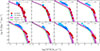 |
Fig. A.1. IR (red circles) and UV (cyan circles) SFRFs (in complete SFR bins) compared to the SFRF obtained by converting the SMF using the MS. The magenta SFRF is obtained using the MS by Speagle et al. (2014), while the green area is from Popesso et al. (2023). |
Appendix B: Details on the models
We report in this Appendix (Tables B.1 and B.2) the main details, mostly on the dust and SF treatment, of the hydrodynamical simulations and SAMs used as a comparison in this work.
Key properties of the hydrodynamical simulations considered in this work, including star formation (SF) parameters.
Key properties of the semi-analytical models considered in this work, including star formation parameters.
All Tables
Key properties of the hydrodynamical simulations considered in this work, including star formation (SF) parameters.
Key properties of the semi-analytical models considered in this work, including star formation parameters.
All Figures
|
Fig. 1. Normalized density distributions of the IR-SFR obtained through SED fitting for the full A3COSMOS sample (cyan) and for the subsample used in this work (teal). |
| In the text | |
|
Fig. 2. Upper panel: UV and IR SFRFs at different redshifts. Data points are plotted in cyan (UV) and red (IR), with best-fit curves shown as blue (UV) and red (IR). Lower panel: Product of volume density (Φ) and SFR in each redshift bin, which is integrated to obtain the SFRD. The UV (blue area) and the IR (red area) SFR density distributions are compared at different redshifts as a function of the SFR. Both curves are normalized so that the UV peak is at 1. |
| In the text | |
|
Fig. 3. Combined SFRF best-fit. The UV and IR data points are the same as in Figure 2. Open blue circles indicate the UV points excluded from the combined fit. The combined best-fit is shown as a yellow shaded region, corresponding to the 16th and 84th percentiles from the MCMC analysis. |
| In the text | |
|
Fig. 4. Observed SFRF compared with predictions from simulations and SAMs. The yellow region represents the observed data used for the fit. The black curve indicates the best fit. The dashed purple line represents the SFRF from the EAGLE simulation, the dashed pink curve shows the result from the SIMBA simulation, and the magenta line corresponds to IllustrisTNG (Katsianis et al. 2017a, 2021a). The lime-green and green dotted curves show the predictions from the GAEA SAM by Hirschmann et al. (2016) and Fontanot et al. (2020), respectively. Finally, the dotted cyan curves show the predictions by Parente et al. (2023). |
| In the text | |
|
Fig. 5. Fraction of the combined SFRD recovered by UV (light blue and blue histograms) and IR (red histograms) data as a function of redshift. The filled blue histograms show the fraction recovered by the observed UV (i.e., without dust correction), while the light-blue dashed histograms correspond to the dust-corrected UV. We note that the UV and IR fractions do not sum to unity, since each SFRD is obtained by integrating the respective best-fit SFR function. |
| In the text | |
|
Fig. 6. Upper panel: SFRD obtained by integrating the combined SFRFs in each redshift bin (yellow area), compared to IR and UV results from the literature (shown as red and blue open symbols, respectively). Lower panel: SFRD compared with predictions from the models discussed in this work. The color code for the models is the same as in Figure 4. |
| In the text | |
|
Fig. 7. Fit to the total SFRD using the functional form by Madau & Dickinson (2014). The best fit to our data is shown as the dashed orange line with yellow error bands. The Madau & Dickinson (2014) fit is plotted in black. A similar fit from Fujimoto et al. (2024) is shown as the dotted blue line, while the shaded green area represents the combined SFRD estimated by Burgarella et al. (2013). In the upper-right corner, we display the best-fit values of the free parameters of Equation (11). |
| In the text | |
|
Fig. A.1. IR (red circles) and UV (cyan circles) SFRFs (in complete SFR bins) compared to the SFRF obtained by converting the SMF using the MS. The magenta SFRF is obtained using the MS by Speagle et al. (2014), while the green area is from Popesso et al. (2023). |
| In the text | |
Current usage metrics show cumulative count of Article Views (full-text article views including HTML views, PDF and ePub downloads, according to the available data) and Abstracts Views on Vision4Press platform.
Data correspond to usage on the plateform after 2015. The current usage metrics is available 48-96 hours after online publication and is updated daily on week days.
Initial download of the metrics may take a while.