| Issue |
A&A
Volume 705, January 2026
|
|
|---|---|---|
| Article Number | A208 | |
| Number of page(s) | 10 | |
| Section | Cosmology (including clusters of galaxies) | |
| DOI | https://doi.org/10.1051/0004-6361/202555726 | |
| Published online | 20 January 2026 | |
Gravity-selected galaxy clusters: A tight mass-richness relation and an unclear Compton Y-richness trend
1
INAF–Osservatorio Astronomico di Brera Via Brera 28 20121 Milano, Italy
2
INAF–Osservatorio Astronomico di Padova Vicolo Osservatorio 5 35122 Padova, Italy
★ Corresponding author: This email address is being protected from spambots. You need JavaScript enabled to view it.
Received:
29
May
2025
Accepted:
7
November
2025
Abstract
This paper, the third in a series, investigates the scaling relations between optical richness, weak-lensing mass, and Compton Y for a sample of galaxy clusters selected purely by their gravitational effect on the shapes of background galaxies. This selection method is uncommon, as most cluster samples in the literature are selected based on signals originating from cluster baryons. We analyze a complete sample of 13 gravity-selected clusters at intermediate redshifts (with 0.12 ≤ zphot ≤ 0.40) with weak-lensing signal-to-noise ratios exceeding 7. We measured cluster richness by counting red-sequence galaxies, identifying two cases of line-of-sight projections in the process, later confirmed by spectroscopic data. Both clusters are sufficiently separated in redshift that richness contamination can be easily mitigated, since the two red sequences do not blend with each other. We find an exceptionally tight richness–mass relation using our red-sequence-based richness estimator, with a scatter of ∼0.05 dex, smaller than the intrinsic scatter of Compton Y with mass for the same sample. The lower scatter highlights the effectiveness of richness compared to Compton Y. No outliers are found in the richness-mass scaling, even when the cluster with a mass likely affected by projection effects is included in the sample. In the Compton Y-richness plane, the data do not delineate a clear trend. The limited sample size is not the sole reason for the unclear relation between Compton Y and richness, since the same sample, with identical richness values, exhibits a highly significant and tight mass-richness correlation.
Key words: galaxies: clusters: general / galaxies: clusters: intracluster medium
© The Authors 2026
 Open Access article, published by EDP Sciences, under the terms of the Creative Commons Attribution License (https://creativecommons.org/licenses/by/4.0), which permits unrestricted use, distribution, and reproduction in any medium, provided the original work is properly cited.
This article is published in open access under the Subscribe to Open model. This email address is being protected from spambots. You need JavaScript enabled to view it. to support open access publication.
1. Introduction
The mass of galaxy clusters is a fundamental quantity in both astrophysics and cosmology. Precise mass estimates are crucial for a range of applications, including studies of the physical processes shaping the intracluster medium (ICM) and galaxy populations, cosmological tests using the cluster mass function, and the comparison of clusters with different properties, since more massive clusters tend to host more galaxies, gas, and dark matter. Comparisons must be properly scaled by mass. However, cluster mass is not directly observable. The two primary methods that directly measure mass, weak gravitational lensing, and the caustic technique, are observationally expensive: weak lensing (Tyson et al. 1990; Kaiser & Squires 1993; Schneider 1996) requires the precise measurement of small distortions in the shapes of faint, distant galaxies, while the caustic method (e.g., Diaferio & Geller 1997) demands dense spectroscopic sampling to trace escape velocities.
Forthcoming wide-field optical and near-infrared surveys, such as Euclid (Laureijs et al. 2011), Roman (Green et al. 2012), Rubin Observatory LSST (LSST Science Collaboration 2009), and the China Space Station Telescope (CSST, Zhan 2011), will detect millions of clusters over large areas of the extragalactic sky. However, only a small fraction will have direct mass estimates, and those that do will predominantly lie at lower redshifts. For instance, Euclid is expected to detect nearly two million clusters peaking at z ∼ 0.8, with a tail extending to z = 2 (Sartoris et al. 2016); however, only about 30 thousands (1.5%) will have a weak-lensing signal-to-noise above 5, and these will be limited to z < 0.7, with mostly at 0.2 < z < 0.4 (Andreon & Hurn 2010).
Given the lack of direct mass measurements for the bulk of cluster samples in optical and near-infrared surveys, robust and efficient mass proxies that can be derived from this type of data are essential. Galaxy cluster richness, particularly when restricted to red-sequence galaxies largely devoid of gas, has proven to be a reliable and observationally inexpensive mass proxy. Its robustness stems from the luminosity and color of red galaxies being minimally affected, if at all, by interactions, cluster mergers, and, in general, by the cluster dynamical state. Moreover, photometric redshifts and red-sequence colors (e.g., Gladders & Yee 2000) enable the detection of projected structures along the line of sight, provided the redshift separation exceeds Δz = 0.02 (Andreon & Hurn 2010).
Most studies adopting a richness–mass relation assume a linear relation in log quantities without outliers (e.g., Saro et al. 2015; Jimeno et al. 2018; Costanzi et al. 2019; Bellagamba et al. 2019; Bleem et al. 2020; Singh et al. 2025; Ghirardini et al. 2024). Empirically, very few outliers are known: none among 53 clusters in Andreon & Hurn (2010), one among 11 in Foëx et al. (2012), none among 23 in Andreon & Congdon (2014), and only two dubious cases in samples of 39 and ∼20 clusters in Andreon (2015) and Mantz et al. (2016), respectively. Andreon et al. (2025, hereafter Paper I) reported one outlier in a sample of four. Notably, all but Paper I rely on X-ray-selected samples, whereas future surveys such as Euclid, Roman, Rubin, and CSST will select clusters using galaxy overdensities. X-ray selection introduces biases (e.g., Vikhlinin et al. 2009; Andreon et al. 2011, 2016, 2017).
It is therefore valuable to characterize the richness–mass scaling relation in a sample that is not selected via the ICM. This is the first aim of our paper, where we analyze the gravity-selected sample of Andreon & Radovich (2025, hereafter Paper II), using the very same richness definition as that adopted in the Euclid cluster pipeline (Euclid Collaboration: Mellier et al. 2025).
A second aim of this paper is to investigate the Sunayev-Zeldovic (SZ hereafter) signal–richness scaling relation, where the SZ signal is often loosely referred to as mass. Current findings are inconclusive, due to the limited data and heterogeneous definitions of richness and SZ observables. Gonzalez et al. (2019) identified outliers in the SZ-richness relation, two of which are known mergers with suppressed Compton-Y values. Di Mascolo et al. (2020) expanded the sample and argued that these outliers may simply reflect statistical scatter in a poorly sampled relation and further proposed that two of their own clusters might be genuine outliers. Their analysis is complicated by the spatial filtering present in their data, which forces the extrapolation of Compton Y to poorly sampled spatial scales. Orlowski-Scherer et al. (2021) also reported evidence of two populations in this plane, but as detailed in Paper II, it is to be verified whether their systems without an SZ signal are genuine clusters or line-of-sight projections misidentified as single clusters. Again, some studies (e.g., Grandis et al. 2021; Bleem et al. 2020) assume a Gaussian scatter of the SZ observable and richness with mass and as a consequence, a Gaussian scatter between the SZ observable and richness.
Throughout this paper, we use the term baryon in the astronomical sense, including electrons, which are responsible for both thermal bremsstrahlung emission and the SZ effect. We assume ΩM = 0.3, ΩΛ = 0.7, and H0 = 70 km s−1 Mpc−1. Gaussian posteriors are summarized in the form x ± y, where x and y are the mean and standard deviation. Non-Gaussian posteriors are summarized as  , where (x − z),x, and x + y are the (16, 50, 84) percentiles. All logarithms are in base 10.
2. Sample, measurements, and results
2.1. Sample
The sample analyzed in this study is identical to that used in Paper II. It is a purely gravity-selected sample, constructed from the shear-peak list produced by Oguri et al. (2021), from which we selected a complete sample formed by the 13 clusters with photometric redshifts in the range 0.12 ≤ z ≤ 0.4 and a weak-lensing signal-to-noise ratio greater than 7. This high threshold ensures that the Eddington (1913) correction and its associated uncertainty are negligible. Spectroscopic redshifts are derived in Paper II from SDSS DR18 spectroscopic data (Almeida et al. 2023). Paper II also derives the spherical Compton-Y parameter within r200 using the ACT Compton-y map (Coulton et al. 2024).
The analysis presented in the following sections of our paper shows that the weak-lensing mass of O26 is likely affected by projection effects; therefore, this object should be treated with caution. For safety, we excluded it from the reference sample, although we include O26 in all plots and reinsert it in our sample when testing the (negligible) effect of ignoring or including this object. When excluded, O26 is removed due to its likely affected weak-lensing mass, while its richness measurement remains viable and is calculated. Since the exclusion is unrelated to richness, the sample without O26 continues to be gravity-selected, and our analysis does not need to account for a never-applied richness selection.
2.2. Weak-lensing masses
Cluster masses were estimated in Paper II by fitting the tangential shear profile, derived from the HSC DR1 shape catalog (Mandelbaum et al. 2018), using a Navarro et al. (1997) model over a radial range of 0.35–3.5 Mpc. This range was selected to mitigate the effects of dilution, mis-centering, deviations from the weak-lensing regime, and contamination from neighboring clusters and large-scale structures. The fitting procedure incorporated the concentration–mass relation of Dutton & Macciò (2014), assuming uniform priors on the logarithm of the concentration, and used the Tinker et al. (2008) mass function to account for Eddington (1913) bias. An intrinsic scatter of 20% in the lensing signal was included to account for cluster elongation, triaxiality, and correlated halos. Further methodological details are provided in Papers I and II.
Figure 1 presents the weak-lensing signal-to-noise maps for the four clusters individually discussed in our paper, based on the Schirmer et al. (2004) S-statistics and convolved with a Gaussian filter of σ = 2 arcmin for display purposes only (see Radovich et al. 2008 for details). O26 is primarily identified in Oguri et al. (2021) as the cluster with coordinates (336.2271,−0.3654) with zphot = 0.141. Using SDSS spectroscopic data, we confirmed in Paper II that the spectroscopic redshift is z = 0.142. This cluster is about 100 arcsec south of the weak-lensing peak shown in Fig. 1, which is co-aligned with X-ray emission (measured using a short Chandra exposure targeting a different object, ObsID 3962). The latter cluster has a spectroscopic redshift (measured from the brightest cluster galaxy and a few other galaxies) of z = 0.315. We now adopt the latter cluster as the primary identification; it was previously the secondary identification in Oguri et al. (2021). Figure 2 shows the revised tangential shear profile for cluster O26 after center and redshift change. The inferred mass changes by approximately 1σ, from log M/M⊙ = 14.22 ± 0.22 to log M/M⊙ = 14.45 ± 0.21. However, the shear signal is likely contaminated by the cluster initially identified as O26 because of its low angular separation and similar mass, as discussed later.
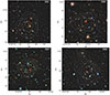 |
Fig. 1. True-color (grz) HSC images with overlaid contours of the weak-lensing S-map, serving as a proxy for signal-to-noise, convolved with a Gaussian filter of σ = 2 arcmin for display purposes. The red and cyan crosses mark the positions of the target cluster and other clusters (present in O26 and O40 panels), respectively. The true-color images are taken from https://www.legacysurvey.org/viewer. |
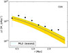 |
Fig. 2. Binned tangential shear profile of the O26 cluster, incorporating the updated identification. The solid line, with yellow shading, represents the mean model and the 68% uncertainty region. The uncertainty in the model also includes intrinsic scatter, while the plotted error bars account only for shape noise and large-scale structure. The dashed cyan line represents the maximum likelihood estimate (MLE), which is biased. The triangle denotes the 2σ upper limit. |
Approximately 5.6 arcmin north of O40 (corresponding to about 1 Mpc at the cluster redshift), lies a known cluster, RM J091409.2+014405.3 (Rozo et al. 2015; Radovich et al. 2017). Given its limited impact on the shear map, particularly after projecting the shear tangentially to O40, we do not expect it to significantly contaminate the tangential shear profile of O40. Nonetheless, we investigate this possibility. Figure 3 compares the expected tangential shear profile of a cluster with log M/M⊙ = 14.5 (i.e., the mass measured for O40) along with the contribution from a background cluster at a projected separation of 1 Mpc, assumed to have log M/M⊙ = 14.7 at z = 0.389. The assumed redshift corresponds to the spectroscopic redshift of RM J091409.2+014405.3 determined using SDSS DR18 data (Almeida et al. 2023) as for the targets. The estimated mass corresponds to the measured richness-based mass of the contaminant, derived as described below for the targets. The contaminating cluster contributes negligibly to the total shear, and only at radii greater than 1 Mpc, as expected. This contamination can, therefore, be safely neglected.
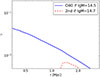 |
Fig. 3. Expected O40 tangential shear profile if O40 had the fitted mass value (log M/M⊙ = 14.5), and of a log M/M⊙ = 14.7 cluster located 5.5 arcmin from O40. The figure demonstrates the negligible contribution of the contaminating cluster. |
2.3. Richness measurements
Cluster richnesses were derived using photometry from the third HSC data release (Aihara et al. 2022), following the methodology of Paper I, which itself is based on Andreon (2015, 2016) with minor updates; it is one of two richness estimates adopted by Euclid. Briefly, galaxies located on the red sequence brighter than the passively evolved threshold of MVe = −20 mag were counted within a radius r200. Our operational definition of “on the red sequence” includes galaxies within 0.1 mag redward and 0.2 mag blueward of the color–magnitude relation, with two exceptions discussed below. The color of the red sequence was self-calibrated from the data, as described in Paper I. We used Kron magnitudes as proxies for total fluxes and employed 1.1 arcsec aperture photometry, measured on PSF-matched images to 1.1 arcsec for color estimation (PSF stands for Point Spread Function). The contribution of background and foreground galaxies was estimated using an annulus between 3 and 7 Mpc, with corrections for contamination by unrelated structures. To minimize bias, the annulus was divided into octants, and the two with the highest and the two with the lowest galaxy counts were excluded from the background estimate.
We computed two richness estimates: (i) the reference richness, n200, WL, measured within the weak-lensing radius r200, WL and centered on the Oguri et al. (2021) cluster coordinates (revised by us for O26); and (ii) an additional richness, n200, A16, derived iteratively using a radius–richness scaling relation calibrated on clusters with known masses (Andreon 2015), including evolutionary corrections. The aperture for the latter is centered on the barycenter of the galaxy distribution, iteratively determined from the spatial distribution of galaxies within a 1.0 Mpc radius, as described by Andreon (2016) and in Paper I. While n200, WL shares the radius and center with the weak-lensing mass measurement, n200, A16 does not.
The richness determination identifies two cases of contamination from other structures along the line of sight via the presence of bimodal color distributions. The redder peak of the O32 and O26 color distributions corresponds to the expected color of the red sequence at the target redshift (see Fig. 4 for O32). Regarding O32, spectroscopy (DESI Collaboration 2025) confirms that the redder peak originates from galaxies at the cluster redshift, while the bluer peak (approximately 0.2 mag bluer) comprises galaxies unrelated to O32. Among the 21 galaxies with a spectroscopic redshift in this secondary peak, none are at the cluster redshift; many are at z = 0.136. Since the contamination occurs at a lower redshift than the target cluster, it was sampled down by about 2.2 magnitudes fainter than the MVe = −20 mag threshold adopted for O32, leading to a large peak in the color distribution (see Fig. 4). Additionally, the adopted filters are appropriate for the O32 cluster but sample redward of the Balmer break for the foreground population, resulting in a narrow color distribution of the contaminants because galaxies with different stellar ages exhibit similar colors in band pairs redder than the Balmer break (Fukugita et al. 1995; Frei & Gunn 1994). As for the target, we measured the richness of the O32 cluster, and its richness-based mass following Andreon (2016), as updated in Sec. 2.5. We found it to be < 1 × 10¹⁴ M⊙ smaller than the error on O32 mass; therefore, this contamination is negligible for the weak-lensing mass estimation. Regarding richness, removing the contamination is sufficient by adopting a stricter color selection: galaxies must lie no more than 0.1 mag blueward of the red sequence (instead of the default 0.2 mag).
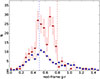 |
Fig. 4. Color distribution of galaxies within r200,wl (red histogram) and in a control area (normalized to the cluster solid angle, blue histogram) for O32. The vertical lines indicate the expected color range of the red sequence. The peak on the right corresponds to the color expected for the cluster redshift, while the second peak represents a contaminating structure along the line of sight spectroscopically confirmed at z = 0.136 (see text for details). For O32, the color range was reduced by 0.1 mag on the blue side to exclude this contamination. Only galaxies brighter than MVe = −20 mag, assuming all galaxies are at the O32 redshift, are considered, which boosts the low redshift contamination. |
O26 is contaminated by the foreground optical cluster originally identified as O26 in Oguri et al. (2021). This results in a similarly bimodal color distribution. In this case, we also used a stricter color selection to measure the richness. However, the richness-based mass of both the target and the contaminant turned out to be quite similar, each having a richness-based mass of about log M/M⊙ = 14.5, making the foreground contamination non-negligible in the weak-lensing estimation (see Fig. 5). Therefore, in our reference analysis, we removed O26 from our cluster sample used for scaling relations, reinserting it to check the sensitivity of our conclusions to its inclusion. As mentioned, dropping this object did not alter the gravity-selected nature of our sample. We verified that applying this stricter color selection to the rest of the cluster sample would not alter their measured richness values.
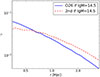 |
Fig. 5. Expected O26 tangential shear profile with the fitted mass value (log M/M⊙ = 14.5), and for a log M/M⊙ = 14.5 cluster located 100 arcsec away. The figure demonstrates the potentially large contribution of the contaminating cluster. |
The derived richness values and the cluster barycenters are listed in Table 1. The mean (log) richness error is 0.07 dex. The two richness estimates (with fixed or to-be-determined center and radii) are in strong agreement, differing on average by 6 ± 10%, while their mean statistical uncertainty is 19%. The cluster centers reported by Oguri et al. (2021) and the galaxy barycenters computed in this work are also highly consistent: in nine out of 13 cases, the positional offset is ≤0.1 Mpc (see Table 1). In the remaining cases, the offsets reflect differences in center definitions. For instance, the offset observed for O27 arises from the lack of spherical symmetry in this cluster, which, as discussed below, experiences a merger. Even in cases where the centers differ, the richness estimates remain consistent to within < 1σ. This robustness is due to the small positional offsets compared to the aperture size used for richness measurement. Moreover, the radial richness profile has a shallow slope near r200, making richness relatively insensitive to small shifts in center position.
Cluster sample and summary of analysis results.
To assess the covariance introduced by using a common measurement radius for both the mass and the n200, WL richness, we performed measurements at different radii in steps of ![Mathematical equation: $ \sqrt[3]{1.2} \, r_{\mathrm{200,WL}} $](/articles/aa/full_html/2026/01/aa55726-25/aa55726-25-eq2.gif) . The results indicate that the covariance induced by the shared radius is subdominant compared to the richness measurement uncertainty. Consequently, this source of covariance is not included in our analysis. In Section 2.5, we verify whether the conclusions of this study are affected when adopting the iteratively computed richness, which lacks radial covariance with the weak-lensing mass due to its independently determined radius and center.
. The results indicate that the covariance induced by the shared radius is subdominant compared to the richness measurement uncertainty. Consequently, this source of covariance is not included in our analysis. In Section 2.5, we verify whether the conclusions of this study are affected when adopting the iteratively computed richness, which lacks radial covariance with the weak-lensing mass due to its independently determined radius and center.
2.4. Results using the weak-lensing aperture r200, WL
Figure 6 shows the relation between mass and richness n200, WL measured within the weak-lensing aperture. We fit the sample with a linear relation (between logarithmic quantities), accounting for Gaussian errors on log mass, non-Gaussian errors on richness, and allowing for intrinsic scatter. In particular, since richness is determined from the difference in galaxy counts between cluster and background regions, we model the Poisson fluctuations in both the cluster and background lines of sight by fitting the observed counts in these regions, rather than the derived richness values shown in Figure 6. The fitting approach follows the methodology of Andreon & Hurn (2010), Andreon (2015, 2016), and subsequent studies. Adopting uniform priors on the intercept, slope angle, and intrinsic scatter, we find
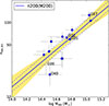 |
Fig. 6. Richness vs. mass scaling relation within r200, WL. The solid line with yellow shading represents the mean richness-mass model with 68% uncertainty, while the dashed corridor indicates the mean model ±1 intrinsic scatter. The clusters discussed in the text are labeled. O26 is not fit due to its likely contaminated weak-lensing mass. Including it in the sample would not alter the scaling relation. In this plot and in Fig. 8, richness errors are approximated as Gaussian for plotting purposes, although their exact distributions are properly accounted for in the fit (see text for details). |
 (1)
(1)
plotted in Fig. 6. The parameters exhibit negligible correlation, as shown in Fig. 7. As detailed in Paper II, the fit does not require modeling the weak-lensing S/N cut, nor does it require modeling the mass function a second time, as the (negligible) Eddington (1913) correction has already been accounted for during the weak-lensing mass estimate. We verified that adding O26 back to the fitted sample would not alter the fit results, as is also evident from its location relative to the fitted scaling.
 |
Fig. 7. Marginal (on the diagonal) and joint (remaining panels) probability distributions of the parameters in Eq. (1). |
Most of the points align along a tight mass-richness scaling relation, with no outliers beyond 2σ, as confirmed by modeling the scatter using a Student’s t-distribution with 10 degrees of freedom. This distribution is robust to the presence of outliers (e.g., Andreon & Hurn 2010) and yields identical scaling parameters.
Formally, the intrinsic scatter around this relation is  dex. However, the derived intrinsic scatter is smaller than the data errors and our analysis assumes that the errors are exact (see Andreon & Hurn 2010 and Andreon 2015 for a fit of the scaling relation with uncertain errors). Therefore, the data constrain only the smallness of the scatter, not its precise 68% error, which can be as low as having a 90% upper limit of 0.05 dex, as found by Andreon (2015) on a different sample.
The tight scaling of richness with mass confirms that the outliers in the Compton Y–mass scaling relation found in Paper II are not due to faulty mass estimates. This is because the mass cannot be incorrect for the Compton Y–mass scaling relation while simultaneously being correct for the richness-mass scaling relation.
The fit of the same data but with swapped dependent and independent variables is
 (2)
(2)
As expected (e.g., Isobe et al. 1990; Andreon & Hurn 2010), the inverse of the slope of the fitted M200|n200 relation, 1/0.68 = 1.5, is not equal to the slope of the inverse n200|M200 relation, 0.85.
2.5. Results using the richness-based aperture r200, A16
Figure 8 presents the mass-richness relation using richness estimates, n200, A16, derived with the galaxy-based r200. This richness adopts an independently derived center and a radius that is uncorrelated with the weak-lensing mass estimate. Therefore, covariance induced by using a common radius for the measurements is absent, as no such common radius exists. This is also relevant for estimating mass from richness, because when richness serves as a mass proxy, both r200 and the center are unknown and must be determined from the galaxy counts.
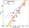 |
Fig. 8. As in Fig. 6, but using richness at the galaxy-derived r200. This richness adopts a radius uncorrelated with the weak-lensing mass estimate and a different cluster center estimate. A tight scaling is also observed here. O26 is not fitted due to its possibly contaminated weak-lensing mass. Including it in the sample would not alter the scaling relation. Note that in this case we fit mass as a function of richness but plot it with mass on the abscissa to facilitate comparison with Fig. 6. The scaling relation seems to differ from the one derived using caustic masses and an X-ray-selected sample (Andreon 2015, dashed line), but interpretation of the cause is premature owing to the degeneracy between sample selection and mass bias (see text for details). |
Fitting the data with the model described above, we find
 (3)
(3)
with a formal intrinsic scatter of  dex, with the caveat that, because the errors on mass and richness are more uncertain than the estimated intrinsic scatter, we can only conclude that the intrinsic scatter is small, but not how close it is to zero. Modeling the scatter with a Student-t distribution, which is robust to the presence of outliers, returns identical scaling parameters. We verified that adding O26 back to the fitted sample would not alter the fit results, as is also evident from its location relative to the fitted scaling relation. The scaling parameters found (Eq. (3)) are nearly identical to those derived using weak-lensing-derived r200 (Eq. (2)), because the two richnesses are nearly identical, as mentioned.
Figure 8 shows a tight scaling relation similar to that obtained using the weak-lensing-derived r200, indicating that our results are unaffected by radius covariance or the precise definition of the center. The tightness of the richness-mass relation confirms and strengthens previous estimates based on caustic masses by Andreon (2016). In fact, the total scatter in the predicted mass (corresponding to the horizontal scatter in Fig. 8) is found to be 0.11 dex, lower than the 0.16 dex measured by Andreon (2016) using caustic masses, making it an even more promising mass proxy.
The intrinsic scatter of our richness estimator, 0.05 dex, is smaller than that of the Compton-Y parameter for the very same sample with shared mass measurements. We fit the (log of) Compton-Y parameter versus log mass data using a linear model with intrinsic scatter and uniform priors on intrinsic scatter, intercept, angle, and log Compton-Y latent values, essentially the hypothesis-parsimonious model of Paper II with dependent and independent variables swapped. We found  , confirming the result found in Paper II: the relation between mass and Compton Y is quite scattered (with a larger sample in Paper III, we concluded that it is not a single relation at all), for our gravity-selected sample. The lower scatter of richness compared to Compton Y highlights the effectiveness of richness as a mass proxy. As noted in Andreon (2015), the quality of a mass proxy also depends on the availability and uncertainty of the proxy observable. Richness has smaller errors (0.07 dex vs. 0.2 dex, median over the same sample), and richness has, by definition, wider availability because no SZ catalog can exist without an optical survey providing an optical identification and photometric redshifts or locations of spectroscopic targets.
O21, named id5 in Paper I, falls close to the richness-mass scaling relations (Figs. 6 and 8) in apparent disagreement with that found in Paper I, in which we reported its predicted mass, based on the n200, WL richness, to be low by 3 sigma from the scaling relation derived from the ICM-selected samples. This is due to two factors: First, in Paper I we compared it to a different scaling relation, based on caustic masses and an X-ray-selected sample, which appears different, as depicted in Fig. 8. The comparison between the two samples is affected by a degeneracy between sample selection and mass bias. Disentangling their effects would require a sample differing in only one of these aspects, which is currently unavailable. Second, the richness value used in Paper I underestimated the cluster richness due to an unfortunate bug: it used the aperture magnitude as total magnitude, which is not total for nearby clusters such as O21. With the newly determined richness (i.e., after the bug correction) the cluster remains an outlier from the compared relation, with log M200, rich/M⊙ = 14.41 ± 0.16, but with lower significance (Fig. 8). The bug does not affect the other clusters in Paper I because of their higher redshifts.
O27 is also known as MACS J0916.1−0023, ACT-CL J0916.1−0024, eFEDS J091610.1−002348, and PSZ2 G231.79+31.48. Based on spectroscopic redshifts (DESI Collaboration 2025), Figure 9 shows that it is a merger in progress, with Δv ∼ 2000 km/s along the line of sight. The merging event is not expected to affect the luminosity of the quiescent galaxy population, as quiescent galaxies are nearly gas-free. Indeed, O27 has the appropriate richness for its weak-lensing mass (Fig. 6), and the inverse is true as well (Fig. 8). A visual inspection of XMM observations and the quantitative analysis of eROSITA data by Sanders et al. (2025) confirm the disturbed morphology expected for an ongoing merger event.
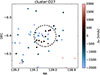 |
Fig. 9. Spatial distribution of galaxies within 3000 km/s from O27, color-coded by velocity offset. The dashed circle indicates 1 Mpc at the cluster redshift. The cluster is clearly undergoing a merger in progress. |
2.6. The unclear Compton Y-richness trend
Once the revised coordinates and redshift were adopted, the O26 Compton-Y parameter changed by less than 1σ, from log Ysph, 200 = −5.31 ± 0.23 to log Ysph, 200 = −5.21 ± 0.31. We checked that using the updated parameters, or removing O26 from the fitted sample, did not alter the Compton Y-mass scaling parameters of Paper II. That analysis, as our current revision, uses the ACT-Planck Compton-Y maps from Coulton et al. (2024) and accounts for the non-Gaussian nature of the errors of log Ysph, 200, among other things.
Figure 10 displays the Compton Y versus richness scaling relation. The data do not seem to correlate with each other: the Pearson correlation coefficient is 0.4 with a p-value of 0.18 (small p-values, for example, < 0.01, indicate the presence of a correlation). For comparison, the Pearson correlation coefficient between richness and mass for the very same 12 clusters with a Compton-Y detection is 0.87 with a p-value of 0.0002, indicating that sample size is not the only reason why the relation between Compton Y and richness seems unclear.
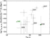 |
Fig. 10. Compton Y-richness scaling relation within r200, WL. The green point and upper limit represent Compton Y–mass outliers. The data do not delineate a clear trend. Clusters discussed in the text are labeled. |
Attempts to fit the data using a range of models, including those with Gaussian and non-Gaussian scatter, single and mixture regressions, and proper handling of Compton-Y errors, which are Gaussian on a linear scale (and therefore not Gaussian in log space), proved highly sensitive to the choice of priors on both parameters and model forms. This sensitivity reflects the limited constraining power of the data, as also indicated by the quoted p-value. As a result, even the form of the Compton Y versus richness relation remains uncertain. Yet, as noted, the same 11 clusters define a remarkably tight richness-mass relation.
The lack of a correlation calls for a closer scrutiny of the data. O19, also known as the CLIO cluster, has its mass estimation and Compton-Y determination scrutinized in Paper II because it is an outlier of the Y–mass scaling relation. The single peak in the color distributions along the O19 line of sight (Fig. 11) confirms the absence of a substantial contamination from other structures, as demonstrated by spectroscopic data and the color-magnitude distribution in Paper II. O19 exhibits a n200, WL richness very close to the mean value expected for its mass (Fig. 6), confirming the mass estimate based on shear data. Discarding O19, the p-value of the Pearson correlation coefficient between richness and Compton Y decreases from 0.18 to 0.03, which is at most weakly suggestive of a correlation and insufficient to establish a statistically significant relationship.
 |
Fig. 11. Color distribution of galaxies within |

Accounting for dusty star-forming galaxies, some of which reside in clusters and are spatially correlated with them, does not substantially alter the measured Compton-Y values. The error-normalized residuals have an average of 0.05 (with Cosmic Infrared Background, CIB, hereafter, -corrected values being slightly lower) and a scatter of about 30% of the measurement uncertainty. The CIB-corrected values were derived from the CIB-deprojected Compton-y maps of Coulton et al. (2024) with β = 1.7 and TCIB = 10.7 K.
3. Conclusions
This paper, the third in a series, investigates the scaling relations between optical richness, weak-lensing mass, and Compton Y for a sample of galaxy clusters selected purely for their gravitational effect on the shapes of background galaxies. Our sample comprises a complete sample of 13 gravity-selected clusters at intermediate redshifts (0.12 ≤ zphot ≤ 0.40) with weak-lensing signal-to-noise ratios exceeding 7, the very same sample used in Paper II to study the Compton Y-mass scaling relation. This selection method is uncommon, as most cluster samples in the literature were selected based on signals originating from cluster baryons.
We measured cluster richness by counting red-sequence galaxies, identifying two cases of line-of-sight projections in the process, later confirmed by spectroscopic data. Both clusters, O26 and O32, are sufficiently separated in redshift that contamination in richness can be readily addressed, as their two red sequences do not blend with each other. Regarding mass estimation, O32 has a foreground structure at Δz ∼ 0.2, whose mass contribution is negligible. O26 by contrast consists of two ∼3 × 10¹⁴ M⊙ clusters separated by ∼1.5 arcmin and Δz ∼ 0.2, whose shear signal is likely affected by projection effects. We excluded this latter system from our reference analysis but also considered it for testing purposes. Since the object exclusion is unrelated to richness, the sample without O26 remains gravity-selected and does not need to account for a never-applied richness selection. We find an extremely tight richness–mass relation using our red-sequence-based richness estimator, with a scatter of ∼0.05 dex, smaller than the intrinsic scatter of Compton Y with mass for the same sample. This lower scatter highlights the effectiveness of richness compared to Compton Y. No outliers are found in the richness-mass scaling, regardless of whether O26 is included in the sample (with the likely contaminated mass). The O27 cluster – a merger in progress – also follows the scaling relation, suggesting that cluster richness is not perturbed during the cluster merger. The tightness of the richness-mass relation supports the accuracy of the weak-lensing mass measurements and reinforces the interpretation from Paper II that two clusters, O40 and O19, are genuine outliers in the Compton Y-mass scaling relation.
In the Compton Y-richness plane, the data do not delineate a clear trend, as indicated by the Pearson correlation coefficient with an insignificant p-value, which makes the fit results sensitive to both the priors on parameters and the fitted model form. The limited sample size is not the sole reason for the unclear relation between Compton Y and richness, since the same sample, with identical richness values, exhibits a highly significant mass-richness correlation.
The upcoming Data Release 1 of the Euclid survey (Euclid Collaboration: Mellier et al. 2025) will enable an expansion of the gravity-selected sample by one to two orders of magnitude. Thanks to its larger size and the uniformity of the richness and mass estimates, it will also allow us to break the degeneracy between sample selection and mass bias that currently limits additional investigations using our sample.
Acknowledgments
SA acknowledges INAF grant “Characterizing the newly discovered clusters of low surface brightness” and PRIN-MIUR grant 20228B938N “Mass and selection biases of galaxy clusters: a multi-probe approach”, the latter funded by the European Union Next generation EU, Mission 4 Component 1 CUP C53D2300092 0006.
References
- Aihara, H., AlSayyad, Y., Ando, M., et al. 2022, PASJ, 74, 247 [NASA ADS] [CrossRef] [Google Scholar]
- Almeida, A., Anderson, S. F., Argudo-Fernández, M., et al. 2023, ApJS, 267, 44 [NASA ADS] [CrossRef] [Google Scholar]
- Andreon, S. 2012, A&A, 546, A6 [NASA ADS] [CrossRef] [EDP Sciences] [Google Scholar]
- Andreon, S. 2015, A&A, 582, A100 [NASA ADS] [CrossRef] [EDP Sciences] [Google Scholar]
- Andreon, S. 2016, A&A, 587, A158 [NASA ADS] [CrossRef] [EDP Sciences] [Google Scholar]
- Andreon, S., & Bergé, J. 2012, A&A, 547, A117 [NASA ADS] [CrossRef] [EDP Sciences] [Google Scholar]
- Andreon, S., & Congdon, P. 2014, A&A, 568, A23 [NASA ADS] [CrossRef] [EDP Sciences] [Google Scholar]
- Andreon, S., & Hurn, M. A. 2010, MNRAS, 404, 1922 [NASA ADS] [Google Scholar]
- Andreon, S., & Radovich, M. 2025, ApJ, 985, 78 (Paper II) [Google Scholar]
- Andreon, S., Trinchieri, G., & Pizzolato, F. MNRAS, 412, 4 [Google Scholar]
- Andreon, S., Serra, A. L., Moretti, A., et al. 2016, A&A, 585, A147 [NASA ADS] [CrossRef] [EDP Sciences] [Google Scholar]
- Andreon, S., Wang, J., Trinchieri, G., et al. 2017, A&A, 606, A24 [NASA ADS] [CrossRef] [EDP Sciences] [Google Scholar]
- Andreon, S., Romero, C., Aussel, H., et al. 2023, MNRAS, 522, 4301 [NASA ADS] [CrossRef] [Google Scholar]
- Andreon, S., Radovich, M., Moretti, A., et al. 2025, MNRAS, 536, 3466 (Paper I) [Google Scholar]
- Bellagamba, F., Sereno, M., Roncarelli, M., et al. 2019, MNRAS, 484, 159 [Google Scholar]
- Bleem, L. E., Bocquet, S., Stalder, B., et al. 2020, ApJS, 247, 1 [CrossRef] [Google Scholar]
- Bocquet, S., Dietrich, J. P., Schrabback, T., et al. 2019, ApJ, 878(1), 55 [Google Scholar]
- Brunner, H., Liu, T., Lamer, G., et al. 2022, A&A, 661, A1 [NASA ADS] [CrossRef] [EDP Sciences] [Google Scholar]
- Chen, Y., Cui, W., Han, D., et al. 2020, Proc. SPIE, 11444, 114445B [Google Scholar]
- Chiu, I.-N., Ghirardini, V., Liu, A., et al. 2022, A&A, 661, A11 [NASA ADS] [CrossRef] [EDP Sciences] [Google Scholar]
- Costanzi, M., Rozo, E., Rykoff, E. S., et al. 2019, MNRAS, 482(1), 490 [CrossRef] [Google Scholar]
- Castignani, G., & Benoist, C. 2016, A&A, 595, A111 [NASA ADS] [CrossRef] [EDP Sciences] [Google Scholar]
- Coulton, W., Madhavacheril, M. S., Duivenvoorden, A. J., et al. 2024, Phys. Rev. D, 109, 063530 [NASA ADS] [CrossRef] [Google Scholar]
- DESI Collaboration (Abdul-Karim, M., et al.) 2025, AJ, submitted [arXiv:2503.14745] [Google Scholar]
- Diaferio, A., & Geller, M. J. 1997, ApJ, 481, 2 [Google Scholar]
- Di Mascolo, L., Mroczkowski, T., Churazov, E., et al. 2020, A&A, 638, A70 [NASA ADS] [CrossRef] [EDP Sciences] [Google Scholar]
- Dutton, A. A., & Macciò, A. V. 2014, MNRAS, 441, 3359 [Google Scholar]
- Eddington, A. S. 1913, MNRAS, 73, 359 [Google Scholar]
- Euclid Collaboration (Mellier, Y., et al.) 2025, A&A, 697, A1 [Google Scholar]
- Foëx, G., Soucail, G., Pointecouteau, E., et al. 2012, A&A, 546, A106 [NASA ADS] [CrossRef] [EDP Sciences] [Google Scholar]
- Frei, Z., & Gunn, J. E. 1994, AJ, 108, 1476 [NASA ADS] [CrossRef] [Google Scholar]
- Fukugita, M., Shimasaku, K., & Ichikawa, T. 1995, PASP, 107, 945 [Google Scholar]
- Ghirardini, V., Bulbul, E., Artis, E., et al. 2024, A&A, 689, A298 [NASA ADS] [CrossRef] [EDP Sciences] [Google Scholar]
- Gladders, M. D., & Yee, H. K. C. 2000, AJ, 120(4), 2148 [NASA ADS] [CrossRef] [Google Scholar]
- Gonzalez, A. H., Gettings, D. P., Brodwin, M., et al. 2019, ApJS, 240(2), 33 [NASA ADS] [CrossRef] [Google Scholar]
- Grandis, S., Bocquet, S., Mohr, J. J., et al. 2021, MNRAS, 507, 4 [Google Scholar]
- Green, J., Schechter, P., Baltay, C., et al. 2012, Wide-Field InfraRed Survey Telescope (WFIRST) Final Report [arXiv:1208.4012)] [Google Scholar]
- Isobe, T., Feigelson, E. D., Akritas, M. G., et al. 1990, ApJ, 364, 104 [NASA ADS] [CrossRef] [Google Scholar]
- Jimeno, P., Diego, J. M., Broadhurst, T., et al. 2018, MNRAS, 478, 638 [NASA ADS] [CrossRef] [Google Scholar]
- Kaiser, N., & Squires, G. 1993, ApJ, 404, 441 [Google Scholar]
- Kluge, M., Comparat, J., Liu, A., et al. 2024, A&A, 688, A210 [NASA ADS] [CrossRef] [EDP Sciences] [Google Scholar]
- Krause, E., Pierpaoli, E., Dolag, K., et al. 2012, MNRAS, 419, 1766 [NASA ADS] [CrossRef] [Google Scholar]
- Liu, A., Bulbul, E., Ghirardini, V., et al. 2022, A&A, 661, A2 [NASA ADS] [CrossRef] [EDP Sciences] [Google Scholar]
- LSST Science Collaboration 2009, LSST Science Book Version 2 [arxiv:0912.0201] [Google Scholar]
- Mandelbaum, R., Miyatake, H., Hamana, T., et al. 2018, PASJ, 70, S25 [Google Scholar]
- Mantz, A. B., Allen, S. W., Morris, R. G., et al. 2016, MNRAS, 456, 4 [Google Scholar]
- Murray, C., Bartlett, J. G., Artis, E., et al. 2022, MNRAS, 512, 4785 [NASA ADS] [CrossRef] [Google Scholar]
- Navarro, J. F., Frenk, C. S., & White, S. D. M. 1997, ApJ, 490, 493 [Google Scholar]
- Oguri, M., Miyazaki, S., Li, X., et al. 2021, PASJ, 73, 817 [NASA ADS] [CrossRef] [Google Scholar]
- Okabe, N., Reiprich, T., Grandis, S., et al. 2025, A&A, 700, A46 [NASA ADS] [CrossRef] [EDP Sciences] [Google Scholar]
- Orlowski-Scherer, J., Di Mascolo, L., Bhandarkar, T., et al. 2021, A&A, 653, A135 [NASA ADS] [CrossRef] [EDP Sciences] [Google Scholar]
- Radovich, M., Puddu, E., Romano, A., et al. 2008, A&A, 487, 55 [NASA ADS] [CrossRef] [EDP Sciences] [Google Scholar]
- Radovich, M., Puddu, E., Bellagamba, F., et al. 2017, A&A, 598, A107 [NASA ADS] [CrossRef] [EDP Sciences] [Google Scholar]
- Rozo, E., Rykoff, E. S., Becker, M., et al. 2015, MNRAS, 453, 38 [NASA ADS] [CrossRef] [Google Scholar]
- Sanders, J. S., Bahar, Y. E., Bulbul, E., et al. 2025, A&A, 695, A160 [NASA ADS] [CrossRef] [EDP Sciences] [Google Scholar]
- Saro, A., Bocquet, S., Rozo, E., et al. 2015, MNRAS, 454, 2305 [Google Scholar]
- Sartoris, B., Biviano, A., Fedeli, C., et al. 2016, MNRAS, 459, 1764 [Google Scholar]
- Schirmer, M., Erben, T., Schneider, P., et al. 2004, A&A, 420, 75 [NASA ADS] [CrossRef] [EDP Sciences] [Google Scholar]
- Schneider, P. 1996, MNRAS, 283, 3 [Google Scholar]
- Singh, A., Mohr, J. J., Davies, C. T., et al. 2025, A&A, 695, A49 [NASA ADS] [CrossRef] [EDP Sciences] [Google Scholar]
- Tinker, J., Kravtsov, A. V., Klypin, A., et al. 2008, ApJ, 688, 709 [Google Scholar]
- Tyson, J. A., Valdes, F., & Wenk, R. A. 1990, ApJ, 349, L1 [CrossRef] [Google Scholar]
- Wik, D. R., Sarazin, C. L., Ricker, P. M., et al. 2008, ApJ, 680, 17 [NASA ADS] [CrossRef] [Google Scholar]
- Vikhlinin, A., Kravtsov, A. V., Burenin, R. A., et al. 2009, ApJ, 692, 2 [Google Scholar]
- Zhan, H. 2011, Sci. Sin. Phys. Mech. Astron., 41, 12 [Google Scholar]
All Tables
All Figures
|
Fig. 1. True-color (grz) HSC images with overlaid contours of the weak-lensing S-map, serving as a proxy for signal-to-noise, convolved with a Gaussian filter of σ = 2 arcmin for display purposes. The red and cyan crosses mark the positions of the target cluster and other clusters (present in O26 and O40 panels), respectively. The true-color images are taken from https://www.legacysurvey.org/viewer. |
| In the text | |
|
Fig. 2. Binned tangential shear profile of the O26 cluster, incorporating the updated identification. The solid line, with yellow shading, represents the mean model and the 68% uncertainty region. The uncertainty in the model also includes intrinsic scatter, while the plotted error bars account only for shape noise and large-scale structure. The dashed cyan line represents the maximum likelihood estimate (MLE), which is biased. The triangle denotes the 2σ upper limit. |
| In the text | |
|
Fig. 3. Expected O40 tangential shear profile if O40 had the fitted mass value (log M/M⊙ = 14.5), and of a log M/M⊙ = 14.7 cluster located 5.5 arcmin from O40. The figure demonstrates the negligible contribution of the contaminating cluster. |
| In the text | |
|
Fig. 4. Color distribution of galaxies within r200,wl (red histogram) and in a control area (normalized to the cluster solid angle, blue histogram) for O32. The vertical lines indicate the expected color range of the red sequence. The peak on the right corresponds to the color expected for the cluster redshift, while the second peak represents a contaminating structure along the line of sight spectroscopically confirmed at z = 0.136 (see text for details). For O32, the color range was reduced by 0.1 mag on the blue side to exclude this contamination. Only galaxies brighter than MVe = −20 mag, assuming all galaxies are at the O32 redshift, are considered, which boosts the low redshift contamination. |
| In the text | |
|
Fig. 5. Expected O26 tangential shear profile with the fitted mass value (log M/M⊙ = 14.5), and for a log M/M⊙ = 14.5 cluster located 100 arcsec away. The figure demonstrates the potentially large contribution of the contaminating cluster. |
| In the text | |
|
Fig. 6. Richness vs. mass scaling relation within r200, WL. The solid line with yellow shading represents the mean richness-mass model with 68% uncertainty, while the dashed corridor indicates the mean model ±1 intrinsic scatter. The clusters discussed in the text are labeled. O26 is not fit due to its likely contaminated weak-lensing mass. Including it in the sample would not alter the scaling relation. In this plot and in Fig. 8, richness errors are approximated as Gaussian for plotting purposes, although their exact distributions are properly accounted for in the fit (see text for details). |
| In the text | |
|
Fig. 7. Marginal (on the diagonal) and joint (remaining panels) probability distributions of the parameters in Eq. (1). |
| In the text | |
|
Fig. 8. As in Fig. 6, but using richness at the galaxy-derived r200. This richness adopts a radius uncorrelated with the weak-lensing mass estimate and a different cluster center estimate. A tight scaling is also observed here. O26 is not fitted due to its possibly contaminated weak-lensing mass. Including it in the sample would not alter the scaling relation. Note that in this case we fit mass as a function of richness but plot it with mass on the abscissa to facilitate comparison with Fig. 6. The scaling relation seems to differ from the one derived using caustic masses and an X-ray-selected sample (Andreon 2015, dashed line), but interpretation of the cause is premature owing to the degeneracy between sample selection and mass bias (see text for details). |
| In the text | |
|
Fig. 9. Spatial distribution of galaxies within 3000 km/s from O27, color-coded by velocity offset. The dashed circle indicates 1 Mpc at the cluster redshift. The cluster is clearly undergoing a merger in progress. |
| In the text | |
|
Fig. 10. Compton Y-richness scaling relation within r200, WL. The green point and upper limit represent Compton Y–mass outliers. The data do not delineate a clear trend. Clusters discussed in the text are labeled. |
| In the text | |
|
Fig. 11. Color distribution of galaxies within |
| In the text | |
Current usage metrics show cumulative count of Article Views (full-text article views including HTML views, PDF and ePub downloads, according to the available data) and Abstracts Views on Vision4Press platform.
Data correspond to usage on the plateform after 2015. The current usage metrics is available 48-96 hours after online publication and is updated daily on week days.
Initial download of the metrics may take a while.