| Issue |
A&A
Volume 705, January 2026
|
|
|---|---|---|
| Article Number | A170 | |
| Number of page(s) | 25 | |
| Section | Cosmology (including clusters of galaxies) | |
| DOI | https://doi.org/10.1051/0004-6361/202556061 | |
| Published online | 16 January 2026 | |
Euclid: An emulator for baryonic effects on the matter bispectrum★
1
Department of Physics and Astronomy, University of Waterloo Waterloo Ontario N2L 3G1, Canada
2
Waterloo Centre for Astrophysics, University of Waterloo Waterloo Ontario N2L 3G1, Canada
3
INFN-Sezione di Bologna Viale Berti Pichat 6/2 40127 Bologna, Italy
4
Department of Astrophysics, University of Zurich Winterthurerstrasse 190 8057 Zurich, Switzerland
5
Universität Innsbruck, Institut für Astro- und Teilchenphysik Technikerstr. 25/8 6020 Innsbruck, Austria
6
Donostia International Physics Center (DIPC), Paseo Manuel de Lardizabal 4 20018 Donostia-San Sebastián Guipuzkoa, Spain
7
IKERBASQUE, Basque Foundation for Science 48013 Bilbao, Spain
8
Institute Lorentz, Leiden University Niels Bohrweg 2 2333 CA Leiden, The Netherlands
9
Leiden Observatory, Leiden University Einsteinweg 55 2333 CC Leiden, The Netherlands
10
Department of Physics, Oxford University Keble Road Oxford OX13RH, UK
11
Institute of Astronomy, University of Cambridge Madingley Road Cambridge CB3 0HA, UK
12
Kavli Institute for Cosmology Cambridge Madingley Road Cambridge CB3 0HA, UK
13
University Observatory, LMU Faculty of Physics Scheinerstrasse 1 81679 Munich, Germany
14
Max Planck Institute for Extraterrestrial Physics Giessenbachstr. 1 85748 Garching, Germany
15
Universität Bonn, Argelander-Institut für Astronomie Auf dem Hügel 71 53121 Bonn, Germany
16
Department of Astronomy and Astrophysics, University of California, Santa Cruz 1156 High Street Santa Cruz CA 95064, USA
17
Perimeter Institute for Theoretical Physics Waterloo Ontario N2L 2Y5, Canada
18
School of Mathematics and Physics, University of Surrey Guildford Surrey GU2 7XH, UK
19
INAF-Osservatorio Astronomico di Brera Via Brera 28 20122 Milano, Italy
20
IFPU, Institute for Fundamental Physics of the Universe via Beirut 2 34151 Trieste, Italy
21
INAF-Osservatorio Astronomico di Trieste Via G. B. Tiepolo 11 34143 Trieste, Italy
22
INFN, Sezione di Trieste Via Valerio 2 34127 Trieste TS, Italy
23
SISSA, International School for Advanced Studies Via Bonomea 265 34136 Trieste TS, Italy
24
Dipartimento di Fisica e Astronomia, Università di Bologna Via Gobetti 93/2 40129 Bologna, Italy
25
INAF-Osservatorio di Astrofisica e Scienza dello Spazio di Bologna Via Piero Gobetti 93/3 40129 Bologna, Italy
26
INAF-Osservatorio Astronomico di Padova Via dell’Osservatorio 5 35122 Padova, Italy
27
Dipartimento di Fisica, Università di Genova Via Dodecaneso 33 16146 Genova, Italy
28
INFN-Sezione di Genova Via Dodecaneso 33 16146 Genova, Italy
29
Department of Physics “E. Pancini”, University Federico II Via Cinthia 6 80126 Napoli, Italy
30
INAF-Osservatorio Astronomico di Capodimonte Via Moiariello 16 80131 Napoli, Italy
31
Dipartimento di Fisica, Università degli Studi di Torino Via P. Giuria 1 10125 Torino, Italy
32
INFN-Sezione di Torino Via P. Giuria 1 10125 Torino, Italy
33
INAF-Osservatorio Astrofisico di Torino Via Osservatorio 20 10025 Pino Torinese (TO), Italy
34
INAF-IASF Milano Via Alfonso Corti 12 20133 Milano, Italy
35
INAF-Osservatorio Astronomico di Roma Via Frascati 33 00078 Monteporzio Catone, Italy
36
INFN-Sezione di Roma, Piazzale Aldo Moro, 2 – c/o Dipartimento di Fisica Edificio G. Marconi 00185 Roma, Italy
37
Centro de Investigaciones Energéticas, Medioambientales y Tecnológicas (CIEMAT) Avenida Complutense 40 28040 Madrid, Spain
38
Port d’Informació Científica, Campus UAB C. Albareda s/n 08193 Bellaterra (Barcelona), Spain
39
Institute for Theoretical Particle Physics and Cosmology (TTK), RWTH Aachen University 52056 Aachen, Germany
40
INFN section of Naples Via Cinthia 6 80126 Napoli, Italy
41
Institute for Astronomy, University of Hawaii 2680 Woodlawn Drive Honolulu HI 96822, USA
42
Dipartimento di Fisica e Astronomia “Augusto Righi” – Alma Mater Studiorum Università di Bologna Viale Berti Pichat 6/2 40127 Bologna, Italy
43
Instituto de Astrofísica de Canarias, Vía Láctea 38205 La Laguna Tenerife, Spain
44
Institute for Astronomy, University of Edinburgh, Royal Observatory Blackford Hill Edinburgh EH9 3HJ, UK
45
European Space Agency/ESRIN Largo Galileo Galilei 1 00044 Frascati Roma, Italy
46
ESAC/ESA, Camino Bajo del Castillo, s/n., Urb. Villafranca del Castillo 28692 Villanueva de la Cañada Madrid, Spain
47
Université Claude Bernard Lyon 1, CNRS/IN2P3, IP2I Lyon, UMR 5822 Villeurbanne F-69100, France
48
Institut de Ciències del Cosmos (ICCUB), Universitat de Barcelona (IEEC-UB) Martí i Franquès 1 08028 Barcelona, Spain
49
Institució Catalana de Recerca i Estudis Avançats (ICREA) Passeig de Lluís Companys 23 08010 Barcelona, Spain
50
UCB Lyon 1, CNRS/IN2P3, IUF, IP2I Lyon 4 rue Enrico Fermi 69622 Villeurbanne, France
51
Departamento de Física, Faculdade de Ciências, Universidade de Lisboa, Edifício C8 Campo Grande PT1749-016 Lisboa, Portugal
52
Instituto de Astrofísica e Ciências do Espaço, Faculdade de Ciências, Universidade de Lisboa, Campo Grande 1749-016 Lisboa, Portugal
53
Department of Astronomy, University of Geneva ch. d’Ecogia 16 1290 Versoix, Switzerland
54
Aix-Marseille Université, CNRS, CNES, LAM Marseille, France
55
Jodrell Bank Centre for Astrophysics, Department of Physics and Astronomy, University of Manchester Oxford Road Manchester M13 9PL, UK
56
INFN-Padova Via Marzolo 8 35131 Padova, Italy
57
Aix-Marseille Université, CNRS/IN2P3, CPPM Marseille, France
58
INAF-Istituto di Astrofisica e Planetologia Spaziali, via del Fosso del Cavaliere 100 00100 Roma, Italy
59
INFN-Bologna Via Irnerio 46 40126 Bologna, Italy
60
Institut d’Estudis Espacials de Catalunya (IEEC), Edifici RDIT Campus UPC 08860 Castelldefels Barcelona, Spain
61
Institute of Space Sciences (ICE, CSIC), Campus UAB Carrer de Can Magrans s/n 08193 Barcelona, Spain
62
Universitäts-Sternwarte München, Fakultät für Physik, Ludwig-Maximilians-Universität München Scheinerstrasse 1 81679 München, Germany
63
Institute of Theoretical Astrophysics, University of Oslo P.O. Box 1029 Blindern 0315 Oslo, Norway
64
Jet Propulsion Laboratory, California Institute of Technology 4800 Oak Grove Drive Pasadena CA 91109, USA
65
Department of Physics, Lancaster University Lancaster LA1 4YB, UK
66
Felix Hormuth Engineering Goethestr. 17 69181 Leimen, Germany
67
Technical University of Denmark Elektrovej 327 2800 Kgs. Lyngby, Denmark
68
Cosmic Dawn Center (DAWN), Denmark
69
Max-Planck-Institut für Astronomie Königstuhl 17 69117 Heidelberg, Germany
70
NASA Goddard Space Flight Center Greenbelt MD 20771, USA
71
Department of Physics and Astronomy, University College London Gower Street London WC1E 6BT, UK
72
Department of Physics and Helsinki Institute of Physics, Gustaf Hällströmin katu 2 University of Helsinki 00014 Helsinki, Finland
73
Université Paris-Saclay, Université Paris Cité, CEA, CNRS, AIM 91191 Gif-sur-Yvette, France
74
Université de Genève, Département de Physique Théorique and Centre for Astroparticle Physics 24 quai Ernest-Ansermet CH-1211 Genève 4, Switzerland
75
Department of Physics, University of Helsinki P.O. Box 64 00014 Helsinki, Finland
76
Helsinki Institute of Physics, Gustaf Hällströmin katu 2 University of Helsinki 00014 Helsinki, Finland
77
Laboratoire d’etude de l’Univers et des phenomenes eXtremes, Observatoire de Paris, Université PSL, Sorbonne Université, CNRS 92190 Meudon, France
78
SKAO, Jodrell Bank, Lower Withington Macclesfield SK11 9FT, United Kingdom
79
Centre de Calcul de l’IN2P3/CNRS 21 avenue Pierre de Coubertin 69627 Villeurbanne Cedex, France
80
Dipartimento di Fisica “Aldo Pontremoli”, Università degli Studi di Milano Via Celoria 16 20133 Milano, Italy
81
INFN-Sezione di Milano Via Celoria 16 20133 Milano, Italy
82
Dipartimento di Fisica e Astronomia “Augusto Righi” – Alma Mater Studiorum Università di Bologna via Piero Gobetti 93/2 40129 Bologna, Italy
83
Department of Physics, Institute for Computational Cosmology, Durham University South Road Durham DH1 3LE, UK
84
Université Paris Cité, CNRS, Astroparticule et Cosmologie 75013 Paris, France
85
CNRS-UCB International Research Laboratory, Centre Pierre Binétruy, IRL2007 CPB-IN2P3 Berkeley, USA
86
University of Applied Sciences and Arts of Northwestern Switzerland, School of Engineering 5210 Windisch, Switzerland
87
Institute of Physics, Laboratory of Astrophysics, Ecole Polytechnique Fédérale de Lausanne (EPFL), Observatoire de Sauverny 1290 Versoix, Switzerland
88
Telespazio UK S.L. for European Space Agency (ESA), Camino bajodel Castillo, s/n, Urbanizacion Villafranca del Castillo Villanueva de la Cañada 28692 Madrid, Spain
89
Institut de Física d’Altes Energies (IFAE), The Barcelona Institute of Science and Technology Campus UAB 08193 Bellaterra (Barcelona), Spain
90
European Space Agency/ESTEC Keplerlaan 1 2201 AZ Noordwijk, The Netherlands
91
DARK, Niels Bohr Institute, University of Copenhagen Jagtvej 155 2200 Copenhagen, Denmark
92
Space Science Data Center, Italian Space Agency via del Politecnico snc 00133 Roma, Italy
93
Centre National d’Etudes Spatiales – Centre spatial de Toulouse 18 avenue Edouard Belin 31401 Toulouse Cedex 9, France
94
Institute of Space Science, Str. Atomistilor, nr. 409 Măgurele Ilfov 077125, Romania
95
Dipartimento di Fisica e Astronomia “G. Galilei”, Università di Padova Via Marzolo 8 35131 Padova, Italy
96
Institut für Theoretische Physik, University of Heidelberg Philosophenweg 16 69120 Heidelberg, Germany
97
Institut de Recherche en Astrophysique et Planétologie (IRAP), Université de Toulouse, CNRS, UPS, CNES, 14 Av. Edouard Belin 31400 Toulouse, France
98
Université St Joseph; Faculty of Sciences Beirut, Lebanon
99
Departamento de Física, FCFM, Universidad de Chile Blanco Encalada 2008 Santiago, Chile
100
Satlantis, University Science Park Sede Bld 48940 Leioa-Bilbao, Spain
101
Department of Physics, Royal Holloway, University of London Surrey TW20 0EX, UK
102
Instituto de Astrofísica e Ciências do Espaço, Faculdade de Ciências, Universidade de Lisboa Tapada da Ajuda 1349-018 Lisboa, Portugal
103
Cosmic Dawn Center (DAWN)
104
Niels Bohr Institute, University of Copenhagen Jagtvej 128 2200 Copenhagen, Denmark
105
Universidad Politécnica de Cartagena, Departamento de Electrónica y Tecnología de Computadoras Plaza del Hospital 1 30202 Cartagena, Spain
106
Kapteyn Astronomical Institute, University of Groningen PO Box 800 9700 AV Groningen, The Netherlands
107
Infrared Processing and Analysis Center, California Institute of Technology Pasadena CA 91125, USA
108
INAF, Istituto di Radioastronomia Via Piero Gobetti 101 40129 Bologna, Italy
109
Institut d’Astrophysique de Paris 98bis Boulevard Arago 75014 Paris, France
110
ICL, Junia, Université Catholique de Lille, LITL 59000 Lille, France
111
ICSC – Centro Nazionale di Ricerca in High Performance Computing, Big Data e Quantum Computing Via Magnanelli 2 Bologna, Italy
★★ Corresponding author: This email address is being protected from spambots. You need JavaScript enabled to view it.
Received:
23
June
2025
Accepted:
20
October
2025
Abstract
The Euclid mission and other next-generation large-scale structure surveys will enable high-precision measurements of the cosmic matter distribution. Understanding the impact of baryonic processes such as star formation and active galactic nuclei (AGN) feedback on matter clustering is crucial to ensure precise and unbiased cosmological inference. Most theoretical models of baryonic effects to date focus on two-point statistics, neglecting higher-order contributions. This work develops a fast and accurate emulator for baryonic effects on the matter bispectrum, a key non-Gaussian statistic in the nonlinear regime. We employ high-resolution N-body simulations from the BACCO suite and apply a combination of cutting-edge techniques such as cosmology scaling and baryonification to efficiently span a large cosmological and astrophysical parameter space. A deep neural network is trained to emulate baryonic effects on the matter bispectrum measured in simulations, capturing modifications across various scales and redshifts relevant to Euclid. We validate the emulator accuracy and robustness using an analysis of Euclid mock data, employing predictions from the state-of-the-art FLAMINGO hydrodynamical simulations. The emulator reproduces baryonic suppression in the bispectrum to better than 2% for the 68% percentile across most triangle configurations for k ∈ [0.01, 20] h Mpc−1 and ensures consistency between cosmological posteriors inferred from second- and third-order weak lensing statistics. These results demonstrate that our emulator meets the high-precision requirements of the Euclid mission for at least the first data release and provides reliable forecasts of the cosmological information contained in the small-scale matter bispectrum. This underscores the potential of emulation techniques to bridge the gap between complex baryonic physics and observational data, maximising the scientific output of Euclid.
Key words: cosmological parameters / cosmology: theory / dark matter / large-scale structure of Universe
This paper is published on behalf of the Euclid Consortium.
© The Authors 2026
 Open Access article, published by EDP Sciences, under the terms of the Creative Commons Attribution License (https://creativecommons.org/licenses/by/4.0), which permits unrestricted use, distribution, and reproduction in any medium, provided the original work is properly cited.
This article is published in open access under the Subscribe to Open model. This email address is being protected from spambots. You need JavaScript enabled to view it. to support open access publication.
1. Introduction
The European Space Agency mission Euclid (Euclid Collaboration: Mellier et al. 2025) is set to revolutionise our understanding of the large-scale structure (LSS) of the Universe by providing high-precision measurements of cosmic shear, galaxy clustering, and the distribution of matter on cosmological scales (e.g. Heymans et al. 2021; DES Collaboration 2022; Miyatake et al. 2023). These data will enable tight constraints on key cosmological parameters, such as the equation of state of dark energy, the sum of neutrino masses, and the amplitude of primordial density fluctuations (Euclid Collaboration: Mellier et al. 2025).
The classical cosmic shear analysis involves measuring the correlations between galaxy ellipticities as a function of their separation, quantified by the two-point correlation function of the shear (γ-2PCF, e.g. Asgari et al. 2020; Amon et al. 2022; Dalal et al. 2023). This statistic benefits from a well-established theoretical framework, primarily capturing the multiscale variance of the lensing field. However, gravitational collapse introduces non-Gaussian features into the shear field, which are not fully captured by γ-2PCF or other second-order statistics.
As a result, two-point statistics cannot extract all cosmological information, leading to parameter degeneracies, such as the one between the matter density parameter Ωm and normalisation of the power spectrum σ8, which limit constraints to combinations such as  . Various higher-order statistics (HOS) have been proposed in the literature to access additional information (see e.g. Euclid Collaboration: Ajani et al. 2023).
A compelling HOS for probing non-Gaussian features of the LSS is the matter bispectrum (e.g. Bernardeau et al. 2003; Takada & Jain 2003), which captures three-point correlations in the density field and provides complementary information to the widely studied two-point statistics, such as the power spectrum (Halder et al. 2021; Halder & Barreira 2022; Heydenreich et al. 2023; Burger et al. 2024; Gomes et al. 2025).
One of the biggest challenges of HOS is the precise modelling of intermediate to small scales, as HOS extract most additional information on nonlinear scales (Foreman et al. 2020). However, these small scales are heavily affected by baryonic feedback processes, such as gas cooling, star formation, and feedback from active galactic nuclei (AGN), which modify the distribution of matter (van Daalen et al. 2011; Chisari et al. 2018). These processes significantly affect the matter distribution, especially in the nonlinear regime, and must be accounted for in cosmological analyses to avoid biased constraints on fundamental physics (Semboloni et al. 2011; Schneider et al. 2019).
Semboloni et al. (2013) used a halo-model approach to predict the effect of baryons on second-order shear statistics and a perturbation theory approach to predict the effect of baryons on the three-point shear statistics. By applying their method to the OverWhelmingly Large Simulations (Schaye et al. 2010), they found that, similar to second-order statistics, the effect of baryonic processes on third-order statistics is not negligible. Moreover, the two statistics have different sensitivities and dependences on the baryonic parameters. Therefore, the combination of second- and third-order statistics has the potential to self-calibrate baryonic feedback parameters, thus improving constraining power on cosmological parameters and reducing projection effects that arise when marginalising high-dimensional posterior distributions over subsets of parameters, which lead to shifts in one- or two-dimensional marginal posteriors that do not reflect the true structure of the full joint distribution.
Hydrodynamical simulations (e.g. Le Brun et al. 2014; Nelson et al. 2015; Schaye et al. 2015, 2023; McCarthy et al. 2018; Pakmor et al. 2024) offer the most detailed insight into baryonic processes and their effects on the power spectrum (Schaller et al. 2025). However, their computational expense makes exploring the high-dimensional parameter space necessary for future cosmological surveys impractical. A promising method for incorporating baryonic effects involves modifying Gravity-Only (GrO) simulations to mimic the influence of baryons using physically motivated models. These approaches, often referred to as Baryon Correction Models (BCM) or baryonification techniques (Schneider & Teyssier 2015; Schneider et al. 2019; Aricò et al. 2020), are computationally efficient and enable the generation of extensive training sets. Such datasets are instrumental in building fast emulators that predict baryonic suppression as a function of cosmological parameters and a few physically motivated baryonic parameters (Aricò et al. 2021a; Giri & Schneider 2021). Using these tools, the baryonic suppression effects observed in various hydrodynamical simulations can be replicated with percent-level accuracy down to scales of k = 5 − 10 h Mpc−1. Although much progress has been made in emulating baryonic effects on the matter power spectrum, the bispectrum or higher-order statistics have remained comparatively underexplored (see e.g. Aricò et al. 2021b; Anbajagane et al. 2024; Zhou et al. 2025). Given the additional cosmological information contained in the bispectrum and its sensitivity to non-Gaussianities, we develop here, as an essential extension, an emulator that can accurately capture baryonic effects on the bispectrum and is fast enough to be used in Bayesian pipelines.
We do this by expanding the work of Aricò et al. (2021a) on the matter power spectrum and present the first emulator predicting the impact of baryonic processes on the matter bispectrum. We model the relevant baryonic processes employing high-resolution simulations from the BACCO suite (Angulo et al. 2021), post-processed using the baryonification technique developed in Aricò et al. (2020) and the cosmology scaling of Angulo & White (2010). We train deep neural networks to predict the power spectrum and bispectrum of our simulations. Although an emulator of baryonic effects on the power spectrum was already presented in Aricò et al. (2021a), we expand their work to have consistent modelling for the power and bispectrum with a broader parameter space and a scale that extends to larger k-values. We validate these emulators against the FLAMINGO set of high-resolution hydrodynamical simulations (Schaye et al. 2023; Kugel et al. 2023), each incorporating different physical prescriptions for feedback mechanisms, star formation, and gas dynamics. Training on various scales and redshifts ensures that our emulators cover the relevant parameter space for the Euclid mission.
Specifically, we show that our BCM emulator can accurately reproduce the FLAMINGO baryonic effects on the second- and third-order moments of the aperture mass lensing statistic (Jarvis et al. 2004; Schneider et al. 2005) across different configurations of box sizes, particle masses, and strengths of AGN feedback. Furthermore, we combine second- and third-order weak lensing statistics to forecast cosmological constraints under the impact of baryonic effects for a non-tomographic analysis of the Euclid first data release (DR1), quantifying the importance of accounting for baryonic effects in the power spectrum and bispectrum measurements. Our results demonstrate that ignoring baryonic effects could lead to significant biases in interpreting Euclid data or require scale cuts, leading to a severe reduction in constraining power, highlighting the necessity of incorporating these effects into cosmological analyses.
This paper is organised as follows. In Sect. 2, we describe the suites of simulations used for training, validating, and building the emulator. We also describe the GrO simulations used for estimating the Euclid-DR1 covariance matrix for the weak lensing statistics. Section 3 presents the estimation of the bispectrum and its validation. In Sect. 4, we present the training of the BCM emulator of the power spectrum and bispectrum. In Sect. 5, we present the methodology for converting the spectra to weak lensing statistics, which we then use in Sect. 6 to perform the non-tomographic Euclid-DR1 forecast. Finally, we discuss the implications of our findings and potential future extensions in Sect. 7.
2. Simulations
2.1. BACCO simulations
This section describes the BACCO N-body simulations used in this study to build a BCM and quantify the baryonic effects on the matter power and bispectrum. The BACCO simulation suite is specifically designed to provide highly accurate predictions of nonlinear cosmic structure formation as a function of cosmology. The gravitational evolution is computed using L-Gadget3 (Springel 2005; Angulo et al. 2012, 2021), a variant of the Gadget code, with a Plummer-equivalent softening length of ϵ = 5 h−1 kpc. The numerical parameters of the suite, including force and mass resolution, were chosen to achieve convergence at the 1% level in the nonlinear power spectrum at z = 0 and k ∼ 10 h Mpc−1. This setup has been validated against other N-body codes, performing exceptionally well in the Euclid Code Comparison project (Schneider et al. 2016), where it agreed within 2% with most codes up to k ∼ 10 h Mpc−1 (Angulo et al. 2021). Each simulation explores a distinct cosmology, with parameters carefully selected to maximise the coverage of the parameter space when combined with rescaling algorithms (Contreras et al. 2020; Angulo et al. 2021).
In this work, we employ a single gravity-only simulation, a higher-resolution version of TheOne simulation presented in Aricò et al. (2021a). This simulation follows the evolution of 22883 particles of mass mp ≈ 9.55 × 10⁸ h−1 M⊙ within a periodic box of L = 512 h−1 Mpc on a side. We report its cosmology in Table 1. The initial conditions were generated at z = 49 using second-order Lagrangian perturbation theory (2LPT). To minimise cosmic variance, the amplitudes of Fourier modes were fixed to the ensemble average of the linear power spectrum, and we average the summary statistics of two realisations having opposite phases, following the fix and pair approach described by Angulo & Pontzen (2016). The particle catalogue was downsampled by a factor of 43 for computational and memory efficiency. We refer to Aricò et al. (2021b) for detailed convergence tests of resolution and cosmic variance, which show that baryonic effects on the power spectrum and bispectrum produced with the BCM on top of this simulation are converged at the percent level.
Cosmological parameters of the simulations used in this work.
2.1.1. Cosmology rescaling
We explore the cosmological space with the cosmology rescaling algorithm originally proposed in Angulo & White (2010), and further refined by Zennaro et al. (2019) and Contreras et al. (2020). This method computes and applies optimal space and time scale factors, which minimise the linear mass variance between two different cosmologies. Furthermore, after applying these scale factors, one can also correct the large-scale flow motions and the small-scale internal structure of haloes. This algorithm can accurately reproduce the matter and halo clustering in a wide cosmology parameter space, including massive neutrinos and dynamical dark energy, with just a few simulations and in only a few seconds. In this work, we only vary the cosmological parameters Ωm, Ωb, σ8, that have been shown in several works to be the dominant cosmological dependence of baryonic effects, at the level of the matter power spectrum (Schneider et al. 2019; Aricò et al. 2021a). We tested in Appendix C with the BACCO simulation suites that this statement is also valid for the matter bispectrum.
2.1.2. Baryonic correction model
To incorporate the effects of baryonic physics into the mass distribution in GrO simulations, we use the ‘baryonification’ framework (Schneider & Teyssier 2015; Schneider et al. 2019; Aricò et al. 2020). This method applies physically motivated prescriptions for processes such as star formation, gas cooling, and AGN feedback to perturb the positions of particles in gravity-only N-body simulations, thereby modifying the mass distribution.
One key advantage of the baryonification approach is its flexibility in exploring possible modifications to the matter power and bispectrum, accounting for the uncertainties inherent in baryonic physics. Model parameters can be constrained using observational data and tested with hydrodynamical simulations. In this work, we adopt the implementation detailed in Aricò et al. (2021b), which has been successfully tested along with the cosmology rescaling algorithms in simultaneously reproducing the power spectra and bispectra of different hydrodynamical simulations. The model considers several baryonic components. The first component is the bound gas in haloes, whose density is described by a double power law with the transition radius and slopes being free parameters. In this work, we adopt only one free parameter for the bound gas shape, θinn, which represents the inner characteristic scale where the gas slope varies. The outer characteristic scale, θout, was fixed to one, which we verify in Appendix C. Both characteristic scales are reported in units of the halo radius, r200, which in turn is defined as the radius where the halo’s density exceeds the Universe’s critical density by a factor of 200. The bound gas mass fraction, fBG, is parametrised as
 (1)
(1)
where fb = Ωb/Ωm is the cosmic baryon fraction, M200 is the mass inside radius r200, Mc and β are free parameters, and fCG, SG are the central and satellite galaxy stellar mass fractions, respectively. An abundance-matching parametrisation gives the central and satellite galaxy fractions (Behroozi et al. 2013), which have the same parametric form in halo mass and redshifts and their parameters are assumed to be linearly dependent.
In this work, we follow Aricò et al. (2021a) and free only one parameter for the stellar component, M1, z0, cen. This parameter represents the characteristic halo mass for which the central galaxy to halo mass fraction is set to ϵ0, cen = 0.023 at z = 0.
A fraction of the gas is assumed to be ejected by feedback, with a constant density and an exponential cutoff at a given scale, parametrised by a free parameter η. The sum of stellar and gas mass fractions, including the ejected gas, is by construction equivalent to the cosmic baryon fraction fb. We report the priors on the varied BCM parameters in Table 2. Moreover, we fix to a fiducial value the BCM parameters  , which are verified in Appendix C. Finally, we vary the scale factor a = 1/(1 + z) to account for the redshift evolution of baryonic effects. We note that in the following, we write M1 instead of M1, z0, cen.
Priors of the varied BCM parameters.
2.2. FLAMINGO simulations
To test our baryon model, we use the FLAMINGO simulations1, in particular, we use the convergence maps developed and described in Broxterman et al. (2024). A detailed description of the FLAMINGO simulations, their performance, and calibration strategy can be found in Schaye et al. (2023), Kugel et al. (2023), and McCarthy et al. (2023).
The simulations were conducted using the SWIFT hydrodynamic code (Schaller et al. 2024) with the SPHENIX smoothed particle hydrodynamics (SPH) implementation (Borrow et al. 2022). Neutrinos were modelled as massive particles using the method developed by Elbers et al. (2021), which minimises particle shot noise. The simulations incorporate radiative cooling and heating on an element-by-element basis (Ploeckinger & Schaye 2020), star formation following the prescription of Schaye & Dalla Vecchia (2008), and time-dependent stellar mass loss as outlined by Wiersma et al. (2009). Supernova and stellar feedback are implemented kinetically, with neighbouring particles receiving kicks that conserve energy, linear momentum, and angular momentum, as described in Chaikin et al. (2023). Gas accretion onto supermassive black holes and subsequent thermal AGN feedback are modelled based on Booth & Schaye (2009), while kinetic jet feedback follows the AGN jet implementation of Huško et al. (2022), where gas particles are accelerated to a fixed jet velocity aligned with the black hole’s spin.
In this work, we use the box with 2.8 comoving Gpc side length, 50403 dark matter (DM) and baryon particles, and 28003 massive neutrino particles, where the baryonic particle mass is 1.07 × 10⁹ M⊙ and the DM particle mass is 5.65 × 10⁹ M⊙. We use all eight available light cones with different observers. The cosmology of these runs was taken from the Dark Energy Survey year three “3 × 2pt+ All Ext”. ΛCDM cosmology (DES Collaboration 2022), which we denote as ‘D3A’. Complementary to this run, we use all nine baryon descriptions available for the D3A cosmology given in Table 1. These additional runs have the same resolution, but with a box size of 1 Gpc, 18003 baryonic particles, and 10003 massive neutrino particles. We also use the higher and lower mass resolution for the fiducial baryon feedback description (L1_m8 and L1_m10). In the following, we label the gravity-only simulations as ‘GrO’ and those including baryonic feedback as ‘Hydro’.
Baryon descriptions of the FLAMINGO simulations.
At the D3A cosmology, eight runs were calibrated to different galaxy stellar mass functions (M★) and/or gas fractions in clusters (fgas), or they were varied in their overall AGN subgrid feedback prescriptions. The values of the subgrid parameters were adjusted so that the stellar mass function and/or the gas fractions in clusters deviated by specific standard deviations (ΔM★ and Δfgas) from the fiducial model, as shown in the second and third columns of Table 3.
Four of these eight runs focused exclusively on varying gas fractions in clusters. These are identified as fgas± nσ, where n represents the number of standard deviations by which the gas fraction is modified. One additional run was calibrated to match a stellar mass function shifted to a lower mass by 1σ (M*–σ). Another run, labelled M*–σ_fgas–4σ, incorporated variations in both observables. The fiducial AGN feedback model uses a thermal implementation, but two alternative models employ a kinetic jet feedback mechanism. These are denoted as Jet and Jet_fgas–4σ, with the latter targeting reduced gas fractions in clusters. The jet models provide a way to evaluate the sensitivity of observables to variations in subgrid models calibrated to the same data. Lastly, we also make use of a simulation at a lower σ8 than the D3A, which is reported in Table 1, denoted as LS8, and uses the baryon description of the fiducial case L1_m9.
2.2.1. Weak lensing convergence maps
The weak lensing convergence maps κ(ϑ, χ) were created using ray-tracing for each comoving slice, where ϑ refers to the sky coordinates and χ to the comoving distance (Broxterman et al. 2024). A key quantity of gravitational lensing is the magnification or Jacobian matrix defined as
 (2)
(2)
where δK is the Kronecker delta symbol, ,ij = ∂/∂θi ∂/∂θj, β denotes the original position of the ray-traced light ray, and can be computed as an integral along the comoving distance over the gradient of the deflection potential ϕ (see Bartelmann & Schneider 2001). Given the fact that ∇2ϕ = 2κ, we can also express the magnification as
 (3)
(3)
where
 \quad \& \quad \gamma _2(\boldsymbol{\vartheta },\chi ) = \phi _{,12}(\boldsymbol{\vartheta },\chi ). \end{aligned} $$](/articles/aa/full_html/2026/01/aa56061-25/aa56061-25-eq6.gif) (4)
(4)
Based on the magnification matrix derived from density maps in HEALPix format (Górski et al. 2005) with an Nside = 8192, which corresponds to a pixel size of  , the shear signal κ(ϑ, χ) and γ(ϑ, χ) are computed at each pixel location. Next, these convergence maps are combined using the Limber integration (Limber 1954)
![Mathematical equation: $$ \begin{aligned} \kappa (\boldsymbol{\vartheta }) = \int _0^{\chi _\mathrm{max} } {\mathrm{d} } \chi \, n[z(\chi )]\, \frac{{\mathrm{d} } z}{{\mathrm{d} } \chi } \, \kappa (\boldsymbol{\vartheta },\chi ), \end{aligned} $$](/articles/aa/full_html/2026/01/aa56061-25/aa56061-25-eq8.gif) (5)
(5)
where n(z) is the redshift probability distribution of source galaxies given in Euclid Collaboration: Blanchard et al. (2020) as
![Mathematical equation: $$ \begin{aligned} n(z) \propto \left(\frac{z}{z_0}\right) \exp \left[-\left(\frac{z}{z_0} \right)^{3/2}\right] \end{aligned} $$](/articles/aa/full_html/2026/01/aa56061-25/aa56061-25-eq9.gif) (6)
(6)
with  . This redshift distribution is cut at zmax = 3, so that χmax = χ(zmax) and it is normalised.
2.3. Takahashi simulations
As in Burger et al. (2023), we use the Takahashi et al. (2017) simulations to estimate a Euclid-like covariance matrix for our lensing statistics. The simulations by Takahashi et al. (2017) track the nonlinear evolution of 20483 particles within a series of nested cosmological volumes. These volumes start with a side length of L = 450 h−1 Mpc at low redshifts and grow progressively larger at higher redshifts, resulting in 108 full-sky realizations. These simulations were generated using the Gadget-3 N-body code (Springel 2005) and are publicly available2. The cosmological parameters are set to values consistent with WMAP 9 (Hinshaw et al. 2013) and reported in Table 1. Lensing information from these simulations is provided using the Born approximation as 108 full-sky realisations of the convergence and shear, each subdivided into 38 redshift slices in ascending order. To construct a non-tomographic Euclid-DR1-like covariance matrix, we built the weighted average of the first 30 κ maps with ascending redshift. The weight for each redshift slice is measured by integrating the n(z) given in Eq. (6) over the corresponding width of the redshift slice. To have a footprint of roughly 2000 deg2, we divided the 30 full-sky maps into 19 patches, each with a size of roughly 2146 deg2. Shape noise is added to the convergence maps by drawing random numbers from a Gaussian distribution with a vanishing mean and a standard deviation, as follows:
 (7)
(7)
with the pixel area as Apix = 0.18 arcmin2 (Nside = 8192), neff = 30 arcmin−2 as the effective galaxy number density, and shape noise contribution σϵ = 0.3 as stated in Euclid Collaboration: Blanchard et al. (2020).
3. Estimation of the bispectrum
We measure the bispectra and power spectra employing the estimator by Scoccimarro (2000), which defines the bispectrum at k-bins k = {k1, k2, k3} for a simulation of volume V as
 (8)
(8)
where  is the Fourier transform of δ, δD is the Dirac delta distribution, and Δki are the bins of wavenumber ki. The power spectrum is defined by
 (9)
(9)
We further use
 (10)
(10)
so the q-integrals become separable, and we obtain
 (11)
(11)
where Lbox is the length of the simulation box.
 (12)
(12)
The Ikδ(x) can be quickly obtained using Fast Fourier Transforms (FFT). To make feasible the estimation of thousands of spectra using the large grids required for this project, we produced a new implementation of these FFTs that runs on GPUs using the JAX framework, which provides a speed-up of a factor up to 10 with respect to CPUs codes. We publicly released the code BiG (Linke 2024), and show in Appendix A how its estimates for the bispectrum agree with those of CPUs codes such as bskit (Foreman et al. 2020) to better than 0.01%.
This estimator averages over the number of triangle configurations inside a (k1, k2, k3) bin. However, as we are interested in a bispectrum prediction for a specific configuration, we need to define which ‘effective’ triangle configuration any measured bispectrum value corresponds to. Following Oddo et al. (2020), we assign each bin an effective triangle configuration (k1, eff, k2, eff, k3, eff) as
 (13)
(13)
We use these effective ks when creating the emulator in the following sections and, for simplicity, drop the ‘eff’ subscript.
For a given density field with N3 grid points and box length Lbox, the theoretically accessible k modes are k ∈ [2kny, Nkny], where kny = π/Lbox is the Nyquist frequency. In our case, we use N = 858, which leads to kmax = 5.3 h Mpc−1.
To access smaller scales (larger k) without increasing the number of grid points, we use the folding technique presented in Jenkins et al. (1998) and Colombi et al. (2009) and validated for the bispectrum by Aricò et al. (2021b). The particle distribution is ‘folded’ by wrapping particles into a sub-box of side length L/f. Given the same grid and the kny defined in the full box, the new Nyquist frequency is kny′=f kny. In this work, we deploy three foldings f = [1, 2, 4], such that the lowest kmin is 0.0123 h Mpc−1 and the largest kmax is 21.058 h Mpc−1. While combining the three foldings for the power spectrum is straightforward, it is more complicated for the bispectrum. The reason is the missing squeezed triangles, where one of the ki values can only be measured in one folding, while the other ki values are only measurable in the other. In the following, we will allow the emulator to extrapolate to these missing squeezed triangles and validate this on the lensing analysis below, since we currently cannot measure bispectra where all k-configurations fit in a single grid. We also notice that we use the symmetries of the bispectrum B(k1, k2, k3) = B(k2, k3, k1) = B(k3, k2, k1) = B(k3, k1, k2) = B(k1, k3, k2) = B(k2, k1, k3) and that the three sides need to build a triangle, k3 ≤ k1 + k2, which reduces the required measurements. We average the measurements from two opposite-phase realizations to suppress cosmic variance for both power spectra and bispectra. We also subtract the shot noise contribution, which is given as  for the power spectrum and
 ![Mathematical equation: $ B_{\mathrm{sn}}(k_1,k_2,k_3) = \bar{n}^{-2} + \bar{n}^{-1} [P(k_1)+P(k_2)+P(k_3)] $](/articles/aa/full_html/2026/01/aa56061-25/aa56061-25-eq20.gif) for the bispectrum (Peebles 1980). Lastly, we note that we do not deconvolve the window function introduced by the mass assignment scheme, but we checked that the effect is smaller than 0.02% when taking ratios of power spectra and bispectra as in our case.
for the bispectrum (Peebles 1980). Lastly, we note that we do not deconvolve the window function introduced by the mass assignment scheme, but we checked that the effect is smaller than 0.02% when taking ratios of power spectra and bispectra as in our case.
4. Training and validation of the emulator
After measuring the power and bispectra for the GrO and baryonified cases for 1200 nodes distributed in a Latin Hypercube defined by the prior mentioned in Sect. 2, we are ready to build the BCM of the matter power spectrum, S(k) = PHydro/PGrO, and bispectra, R(k) = BHydro/BGrO. For our emulation, we use the CosmoPower neural network (NN) library described in Spurio Mancini et al. (2022). In principle, we could use only the six baryon parameters as input and then interpolate between different k-values. However, we found that it is more convenient, accurate and faster to use also the k-value as input parameters, as this allows us to predict the power and bispectra for any k-values even if they were not measured in the first place. Moreover, in this way, we can clean our training set more efficiently, removing the single B(k1, k2, k3) configurations where B(k1, k2, k3) < 2 Bsn(k1, k2, k3) without having to exclude the whole sampling node. With this procedure, we discard only about 2.5% of the total measurements. We note that we emulate the three-dimensional power spectrum and bispectrum, as opposed to the projected two-dimensional lensing statistics presented in the next sections, to have the flexibility to employ the emulators with different survey setups and projections, without the need to perform the training of more emulators. To further speed up the cosmological analyses, specific emulators for a given survey configuration can be easily developed starting from the ones presented here.
We randomly split our samples of 1200 nodes into 200 points used for testing and 1000 for training. After some iterations, we found that an architecture with four hidden layers and 32 neurons, the Adam optimizer, a mean squared difference loss function, a learning rate that starts at 0.01 and decreases by a factor of 10 if the loss does not improve for 100 epochs of training, and a sigmoid activation, gives the best results. The reason for using as few layers and neurons as possible is to prevent overfitting and attempt to improve the extrapolation to k-values not present in the training. These are, for instance, the squeezed triangles that do not lay in any of the three foldings used and k-values smaller than kmin = 0.0123 h Mpc−1. We note that, while for the power spectrum, the BCM to large scales, k < 0.0123 h Mpc−1, can straightforwardly be set to one, this is not obvious for the bispectrum given its sensitivity to different scales (see Fig. C.2). Therefore, a more complex extrapolation is needed. We implicitly test the accuracy of our NN extrapolation by performing mock analyses using the expected characteristics of Euclid DR1 in Sect. 6, leaving a more thorough explicit test for future works.
We first show the accuracy of our BCM power spectrum emulator in Fig. 1. We find an accuracy on S(k), which we define as ΔS(k) = Semu/Strue − 1, smaller than 0.5% for the 68% percentile, and 3% for the 95% percentile. In other words, this means that 68% of the predictions are better than 0.5% for the power spectrum. We show the accuracy of the bispectrum emulator, defined as ΔR(k) = Remu/Rtrue − 1, in Fig. 2, as a scatter plot where the corresponding 68% and 95% percentiles of ΔR(k) are shown in the upper two and lower two rows, respectively. We used linear interpolation between the measured k-values for a better illustration. The linear extrapolation into regions without measurements, such as the upper left corner for k3 = 5 h Mpc−1, should be taken cautiously. Furthermore, we show in Figs. B.1 and B.2 two different illustrations of the accuracy of the bispectrum emulator, where it is seen that the accuracy is smaller than 2% for the 68% percentile and similar across the different foldings and not particularly problematic at the transition from one folding to the next. Since we took 200 nodes for testing, which are also distributed in a Latin hypercube, the accuracies shown here marginalize over all parameters. However, we found only a minimal dependency of the accuracy towards larger Mc. All the other parameters showed no dependency at all. Overall, we conclude that the emulator is less accurate for very squeezed triangles, especially where the measurement is at the edge of the k-range.
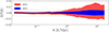 |
Fig. 1. Accuracy of the emulator for baryonic effects on the matter power spectrum. The y-axis is defined as ΔS(k) = Semu/Strue − 1, where S(k) = PBCM(k)/PGrO(k). The horizontal dashed lines show the 0.5% region. |
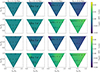 |
Fig. 2. Accuracy of the emulator for baryonic effects on the matter bispectrum R(k). The upper two rows show the lower and upper 68% percentiles of ΔR(k), and the two lower rows show the lower and upper 95% percentiles of ΔR(k). Each column is for a different k3 value, which is by construction larger than k2 and k1 but smaller than k1 + k2. The black circles show the actual location where we have measured B(k1, k2, k3). The background is coloured using a linear interpolation/extrapolation of the percentiles between the measured k-values. |
Remarkably, the overall accuracy of the emulator ΔR(k) is better than 2% for the 68% percentile. In the 95% percentile, the accuracy of isolated triangle configurations seems to be worse than 5%. We have checked that this error arises from residual noise in the measurements. Given that we made sure that our emulator does not overfit this noise, we expect its accuracy to be better than the quoted values in those regions. We stress that these values refer to the accuracy of the emulation process. The underlying physical model was found to reproduce hydrodynamical simulations at a level of 1–3% in Aricò et al. (2021b) down to scales of 5 h Mpc−1. In the next sections, we explore whether this accuracy is enough to provide an unbiased cosmological inference in a Euclid DR1 lensing analysis. For completeness, we show in Figs. C.1 and C.2 how S(k) and R(k) depend on BCM and cosmological parameters.
5. From spectra to weak lensing statistics
This section reviews the second- and third-order weak lensing statistics used to perform a forecast of a non-tomographic analysis of Euclid DR1. For a detailed review of gravitational lensing statistics, we refer to Bartelmann & Schneider (2001), Hoekstra & Jain (2008), Munshi et al. (2008), Bartelmann (2010), and Kilbinger (2015). In this work, we follow the description in Burger et al. (2023) and repeat only the essential details.
5.1. Limber projections of the power spectrum and bispectrum
The projected power- and bispectrum at wavenumber, ℓ, can be computed using the extended Limber approximation (Limber 1954; Kaiser & Jaffe 1997; Bernardeau et al. 1997; Schneider et al. 1998; LoVerde & Afshordi 2008), up to the maximum distance defined by source redshift distribution (Eq. (6)),
![Mathematical equation: $$ \begin{aligned} P_{\kappa \kappa } (\ell ;\Theta )&= \int _0^{\chi _\mathrm{max} } {\mathrm{d} } \chi \;\frac{g^2(\chi )}{a^2(\chi )}\, P\left[\frac{\ell +1/2}{\chi },z(\chi );\Theta \right], \end{aligned} $$](/articles/aa/full_html/2026/01/aa56061-25/aa56061-25-eq21.gif) (14)
(14)
![Mathematical equation: $$ \begin{aligned} B_{\kappa \kappa \kappa }(\ell _1,\ell _2,\ell _3;\Theta )&= \int _0^{\chi _\mathrm{max} }{\mathrm{d} } \chi \; \frac{g^3(\chi )}{a^3(\chi )\,\chi } \nonumber \\&\times B\left[\frac{\ell _1+1/2}{\chi },\frac{\ell _2+1/2}{\chi },\frac{\ell _3+1/2}{\chi },z(\chi );\Theta \right], \end{aligned} $$](/articles/aa/full_html/2026/01/aa56061-25/aa56061-25-eq22.gif) (15)
(15)
where Θ = (Θcos, ΘBCM) is the set of cosmological and BCM parameters. The 3-dimensional P(k, z; Θ) is defined as
 (16)
(16)
and PGrO(k, z; Θcos) is the matter power spectrum computed using Halofit (Takahashi et al. 2012) that depends only on cosmological parameters Θcos, and SBCM = PHydro/PGrO is the BCM described in Sects. 3 and 4 that depends on the BCM parameters ΘBCM. In principle, we can use any implementation of PGro, but we wanted to make use of k > 10 h Mpc−1 and a < 0.4, which the current baccoemu does not provide. In analogy, the 3-dimensional bispectrum B(k, z, Θ) is computed as
 (17)
(17)
where BGrO(k, z; Θcos) is the nonlinear matter bispectrum computed using BiHalofit (Takahashi et al. 2020), and RBCM = BHydro/BGrO is the BCM for the bispectrum.
Lastly, we are only considering closed triangles, ℓ3 = |ℓ1 + ℓ2|, and g(χ) denotes the lensing efficiency and is defined as
 (18)
(18)
with n(χ) = n(z) dz/dχ and n(z) being the redshift probability distribution given in Eq. (6).
5.2. Aperture mass statistics
The aperture mass ℳap at position ϑ with filter radius θap is defined through the convergence κ, as follows:
 (19)
(19)
where Uθap(ϑ′) is a compensated filter such that ∫ℝdϑ′ ϑ′ Uθap(ϑ′) = 0.
We define Uθap(ϑ) = θap−2u(ϑ/θap), denote by  the Fourier transform of u, and use the filter function introduced in Crittenden et al. (2002),
 (20)
(20)
5.3. Modelling aperture mass moments
While the expectation value of the aperture mass ⟨ℳap⟩(θap) vanishes by construction, the second-order (variance) of the aperture mass is nonzero and can be calculated as
 (21)
(21)
Equivalently, the third-order moment of the aperture statistics ⟨ℳap3⟩, can be computed from the convergence bispectrum via (Jarvis et al. 2004; Schneider et al. 2005)
 (22)
(22)
where ℓ3 = |ℓ1 + ℓ2|. In the two lower panels of Fig. C.7, we show how ⟨ℳap2⟩ and ⟨ℳap3⟩ react to changes in the baryonic parameters, while all other parameters are fixed to the fiducial parameters given in Tables 1 and 4. We divide the ⟨ℳapn⟩ predictions by GrO predictions, ⟨ℳapn⟩GrO, to highlight the baryonic effects. As expected, Mc has the largest impact on both ⟨ℳap2⟩ and ⟨ℳap3⟩. This baryonic parameter sets the characteristic halo mass for which half of the gas mass is ejected by feedback, thus regulating the quantity of gas retained in haloes. As expected, the galaxy parameter M1 and the inner gas slope scale θinn have a larger effect on small apertures, whereas the feedback scale η has a larger impact on larger apertures. We note that, comparatively, β has a significantly larger effect on ⟨ℳap3⟩ than on ⟨ℳap2⟩. Looking at the cosmological parameters, we find that the dependence on σ8 is negligible for ⟨ℳap3⟩, but we observe some effect in the second-order statistics. We note that the dependence on Ωm and Ωb can be better captured by their ratio, Ωb/Ωm, which comes from the fact that the impact of the baryon feedback, at fixed strength, depends to zeroth order on the relative amounts of baryons to the dark matter.
Fiducial baryon parameters.
5.4. Modelling convergence correlation functions
Since the ⟨ℳap2⟩ statistics smooth much of the small scales, we decided to add the information from the two-point correlation function ξκ itself, which is defined by
 (23)
(23)
where J0 is the zeroth Bessel function of the first kind. In the lower panel of Fig. C.7, we show how ξκ reacts to changes in the baryonic parameters. As for the ⟨ℳapn⟩ moments, we divide the ξκ predictions by GrO predictions, ξκGrO, to highlight the role of baryons. Similarly as for ⟨ℳap2⟩, we observe that the most important baryonic parameters are Mc and η.
5.5. Flamingofied data vector
In this section, we describe the process of ‘flamingofying’ a GrO reference model. A flamingofied reference model of ⟨ℳapn⟩ is built by scaling the prediction of a GrO model at the cosmology of the corresponding FLAMINGO simulation with the ratio of a hydrodynamic-GrO pair of FLAMINGO simulations
 (24)
(24)
Analogously, we flamingofy the ξκ in the following way
 (25)
(25)
In Figs. 3 and 4, we show in blue the ratio Hydro/GrO of the FLAMINGO measurements for ⟨ℳapn⟩ and ξκ for the L2p8_m9 scenario. Comparing these ratios to the estimated uncertainty in grey indicates which scales are affected by baryonic effects. Furthermore, we show the red dashed line as the best-fitting model to fit the flamingofied reference model if we fix the cosmology to D3A, where we performed a χ2 minimisation for each statistic separately to find the best-fitting parameters. Our BCM model can perfectly fit the flamingofied reference model. This is an encouraging result for the cosmological analysis in the next section.
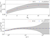 |
Fig. 3. Baryonic effects on ⟨ℳap2⟩ (upper panel) and on ξκ (lower panel), illustrated by ratios of measurements with baryonic physics to GrO measurements. We show with blue triangles the fiducial FLAMINGO measurements, and the grey shaded area represents the Euclid DR1 uncertainty. We overplot with a red dashed line the best-fitting BCM to the flamingofied data vector, found by employing our emulators with fixed cosmological parameters. |
 |
Fig. 4. Same as Fig. 3 but for the ⟨ℳap3⟩ statistics. The x-axis shows different combinations of θap, 1-θap, 2-θap, 3. |
We also show the effects of baryons from the FLAMINGO description L2p8_m9 in each panel. The ⟨ℳapn⟩ in the FLAMINGO and Takahashi simulations are measured by applying Eq. (19), using the Healpy smoothing option. We have decided to use aperture filter radii θap = {2′, 4′, 8′, 16′, 32′}, where the lower value θap = 2′ is constrained by the chosen pixel resolution  of the FLAMINGO/T17 convergence maps. The ξκ in the FLAMINGO and Takahashi simulations are measured with TreeCorr (Jarvis et al. 2004), from
  in 15 logarithmic bins, where the lower edge is determined again by the resolution of the chosen convergence maps.
6. Euclid forecasts
In this section, we perform a non-tomographic Euclid DR1 forecast, where we vary the matter density Ωm, the baryon density Ωb, the normalisation of the power spectrum σ8, and the five baryonic parameters described in Sect 2.1.2. The dependence of these parameters on ⟨ℳapn⟩ and the ξκ are already discussed in Sect. 5 and are shown in Fig. C.7. We have not yet mentioned that the computations of the integrals of these quantities are not efficient enough to perform several Markov Chain Monte Carlo (MCMC) analyses. Therefore, we decided to train another set of emulators on top of the three-dimensional power and bispectrum emulators, which predict the ⟨ℳapn⟩ and ξκ. We computed the ⟨ℳapn⟩ and the ξκ for 2200 points distributed in a Latin hypercube. We estimate the error of the emulation, by building a set of emulators iteratively leaving out from the training 200 of the 2200 points at a time. Since the power and bispectrum are noisy quantities themselves, their noise also propagates into the summary statistics. Furthermore, the integration to ⟨ℳap3⟩ sometimes fails for very squeezed configurations, because we had to limit the number of ℓ values where we compute Bκκκ for the sake of computational speed. Therefore, the emulator error accounts for emulator noise in the summary statistics but also for noise in the power and bispectrum estimations and their subsequent integration. We note that this procedure, however, does not account for possible systematic errors in the emulation or integration. The error of this emulator is less than a tenth of the uncertainty estimated with the Takahashi et al. (2017) simulations. Although this might be neglected, we decided to build an emulator covariance matrix for correctly estimating the posterior, using the 2200 Δm = memu − mtrue predictions and add it to the Takahashi et al. (2017) covariance matrix as
 (26)
(26)
Since the estimated covariance matrix C is a random variable itself, we follow Percival et al. (2022) to compute the Likelihood. Given a data vector d and covariance matrix C of rank nd measured from nr realizations, the posterior distribution of a model vector m(Θ) that depends on nΘ = 12 parameters is
 (27)
(27)
where
![Mathematical equation: $$ \begin{aligned} \chi ^2 = \left[\boldsymbol{m}(\Theta )-\boldsymbol{d}\right]^\mathrm{T} \mathsf C ^{-1} \left[\boldsymbol{m}(\Theta )-\boldsymbol{d}\right]. \end{aligned} $$](/articles/aa/full_html/2026/01/aa56061-25/aa56061-25-eq38.gif) (28)
(28)
The power-law index m is
 (29)
(29)
and B is defined as
 (30)
(30)
and nr = 570 is the number of realizations, nΘ = 8 the number of free parameters, and nd the rank of the covariance matrix. Although nr for Cemu is not clearly defined, we used the same correction for C as we used for CT17. Lastly, we used the nested sampler nautilus (Lange 2023) to perform the inference, employing 2000 live points. We validated the convergence of the posteriors by comparing them with a Hamiltonian Monte Carlo sampler and a standard Metropolis–Hastings algorithm.
To start our investigation of the impact of baryonic feedback, we show in Fig. 5 posteriors on the cosmological parameters S8, Ωm, and Ωb, which we obtain by analysing a synthetic Euclid DR1 data vector built from a combination ξκ, ⟨ℳap2⟩, and ⟨ℳap3⟩. The investigation here is built solely using Halofit, BiHalofit, and the BCM, which means we always know the true input of cosmological and BCM parameters. In the first case (black), we created a data vector using the BCM with the parameters given in Table 4 and analysed it with the GrO model, meaning we turned the BCM off in the modelling. This results in a 2.5σ shift in S8. Substantial scale cuts on small scales are required to avoid such a bias, which we show as the orange contours. In terms of scales these are θ > 8′ for ξκ, θap = 32′ for ⟨ℳap2⟩ and θap, 1 ∈ {16′, 32′} with θap, 2, 3 = 32′ for ⟨ℳap3⟩. However, this drastically reduces the precision on S8 by 8% and by almost 80% on Ωm compared to modelling all five BCM parameters shown as the red contours. We obtain even tighter constraints by fixing these five BCM parameters to their true values, as shown in the blue contours. Having perfect knowledge of baryonic effects results in cosmological constraints almost identical to the case where we used a GrO data vector and analysed it with a GrO model, displayed with purple contours. We will show later that we probably do not need to vary all five BCM parameters for the expected Euclid DR1 uncertainty.
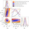 |
Fig. 5. Posteriors of the cosmological parameters S8, Ωm, and Ωb, analysing a synthetic Euclid DR1 joint data vector of second- and third-order weak lensing statistics. We consider several cases. First, a gravity-only (GrO) data vector was analysed with a GrO model (purple contours). We obtain the black contours when baryonic effects are included in the data vector but not in the model. In orange, we illustrate the constraints we get when all elements of the data vector are excluded where the baryonic data vector deviates by more than 0.4σ from the GrO data vector. Lastly, we show the results if the model includes baryonic feedback in red and blue, where we fixed the baryon parameters to the truth in the blue case and marginalised over all five parameters for the red. The grey dashed line indicates the underlying D3A cosmology. |
6.1. Validating the emulator on the FLAMINGO simulations
First, we use a flamingofied data vector estimated from eight light cones of the 2.8 Gpc box that uses the fiducial baryon description (see Sect. 5.5). This test aims to see if the combination of the three different statistics improves the constraining power and check if the BCM is flexible enough to fit the fiducial FLAMINGO simulation. The constraints on both cosmological and baryonic parameters are shown in Fig. 6. This is one of the main results of this paper and shows that our baryon model can describe the modifications due to baryons while resulting in unbiased cosmological results for all three statistics and their joint analysis. We note that ⟨ℳap2⟩ yields similar constraints as ξκ, since both result from integrating the power spectrum, so we decided to show only the combination. Next, we notice that ⟨ℳap3⟩ constrains the cosmological parameters slightly better than the second-order statistics, and furthermore helps breaking parameter degeneracies. Compared to Burger et al. (2024), where second-order statistics were relatively more constraining, we expect that this comes from the fact that we include smaller scales with θap = 2′, where higher-order statistics become more important. We do not show the ‘true’ FLAMINGO values for the BCM parameters. These can be measured in hydrodynamic simulations in principle; however, their measured values are redshift-dependent. Thus, interpreting our constraints is not straightforward since they are weighted in redshift according to our lensing kernel. We leave for future work a thorough test of the BCM parameter constraints, as a correct inference of baryonic physics is essential, for example, in cross-correlations and multi-probes analyses.
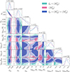 |
Fig. 6. Euclid DR1 forecast, where we used a flamingofied reference data vector (see Sect. 5.5) estimated from the fiducial baryon description of the FLAMINGO simulations with eight light cones of the 2.8 Gpc box. The stated constraints correspond to the joint analysis of second- and third-order statistics. The grey dashed line indicates the underlying D3A cosmology. |
In Fig. 7, we compare the constraining power of second-order and third-order statistics in the Ωm- plane. We highlight the different degeneracy axes of the second- and third-order statistics, which are broken when both are combined, in agreement with Semboloni et al. (2013). Therefore, combining second- and third-order statistics increases the constraining power by 22% for S8 and even 50% for Ωm compared to using second-order statistics alone. Lastly, we also show the case where we discard all the non-equal scale filter radii θap. Interestingly, these non-equal scale filter radii θap play an essential role in the precision and accuracy of cosmological parameters, since discarding them reduces the constraining power by around 16% for S8 and Ωm compared to using all filter combinations. Burger et al. (2023) found that these non-equal scale filter radii are less significant. We interpret this as non-equal scale filter radii being important to constrain the BCM parameters, which in turn helps to constrain cosmological parameters. Another explanation for the discrepancies with Burger et al. (2023) could also lie in the fact that we include the θap = 2′ filter and that we used a different tomographic setup.
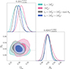 |
Fig. 7. Euclid DR1 forecast, where we used a flamingofied reference data vector (see Sect. 5.5) estimated from the fiducial baryon description of the FLAMINGO simulations with eight light cones of the 2.8 Gpc box. The stated constraints correspond to the joint analysis of second- and third-order statistics. The posteriors are the same as those used in Fig. 6, meaning we marginalised over all BCM parameters. The stated constraints correspond to the joint analysis of second- and third-order statistics (blue contours). The grey dashed line indicates the underlying D3A cosmology. |
Testing only one astrophysical scenario is insufficient to ensure a robust cosmological inference. Therefore, we use all baryon feedback descriptions described in Sect. 2.2. We build flamingofied data vectors as described in Sect. 5.5. We run an MCMC for each baryon feedback description once using only second-order statistics ξκ + ⟨ℳap2⟩ and once combining second- and third-order ξκ + ⟨ℳap2⟩+⟨ℳap3⟩, where we vary all baryon parameters. We present the result as the black symbols in Fig. 8, where the error bars represent the 1σ uncertainties estimated from the MCMC chains. The corresponding best-fitting parameters are shown as the stars, and we notice that the best-fitting parameters are much closer to the truth than the mean, which might indicate non-Gaussian parameter posteriors or significant projection effects. Remarkably, we get unbiased cosmological results for all FLAMINGO flavours and configurations for both the second-order alone and the second- and third-orders combined. This is the most important result of this paper, as it shows that our BCM model is flexible enough to get unbiased results for all FLAMINGO feedback variations. This also shows that the interpolation and extrapolation of our emulators for the BCM power spectrum and bispectrum are sufficient for the current setup. We expect the emulator accuracy requirements to be similar in a tomographic setup, such that our emulators are ready for a Euclid-like DR1 analysis. However, a tomographic analysis might require an explicit redshift dependence on the baryonic parameters. We highlight that the three-dimensional power spectrum and bispectrum emulators developed in this work would remain valid and could be used with parametrised redshift dependencies without creating new training sets or emulators.
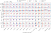 |
Fig. 8. Estimated weighted mean (triangles) and 68% credible intervals from the MCMC chains for all FLAMINGO models described in Sect. 2.2. Since the LS8 and Planck cosmology is different we plot ΔΩm = Ωmbest − Ωmtrue and in analogy ΔS8 and ΔΩb. The different colours show cases where parameters are fixed. The stars indicate the best-fitting parameters resulting from a minimisation process that returns the lowest χ2. The figure is for ξκ + ⟨ℳap2⟩+⟨ℳap3⟩. The corresponding figure for ξκ + ⟨ℳap2⟩ is shown in Fig. C.6. |
6.2. Assessing the importance of the BCM parameters
In this subsection, we exploit a wide range of feedback models of the FLAMINGO suite to assess the importance of each BCM parameter in a cosmological analysis. We aim to find the minimal BCM model required to deliver unbiased cosmological constraints in a Euclid DR1 lensing analysis. Fewer free parameters would help mitigate projection effects and allow for faster convergence of the posteriors. This analysis cannot be straightforwardly generalised to different hydrodynamical simulations and summary statistics. Nevertheless, this section provides us with valuable information about the most important BCM parameters that can capture the large variety of baryonic variations in FLAMINGO, even if care must be taken when fixing one or more baryonic parameters in data analyses.
To perform our test, we fix one or more BCM parameters to the weighted average of the best-fitting parameters over all FLAMINGO flavours and configurations, where the weights are estimated from the 1σ credible intervals of MCMC chains. We report those values in Table 5. Next, we run an MCMC for each scenario, and show the best-fitting values, mean and standard deviation of the marginalised posteriors in Fig. 8. Focusing first on ξκ + ⟨ℳap2⟩+⟨ℳap3⟩, we notice that the best-fitting values, especially for S8, are closer to the truth than the weighted mean of the MCMC, indicating strong projection effects. We find that fixing Mc is particularly bad in some cases, where an incorrect estimation of Mc results in a biased S8 inference. Next, we observe that fixing η leads to small biases for the strongest feedback descriptions (jet fgas–4σ and fgas–8σ). Fixing either M1 or β does result in unbiased results for all scenarios, which is not surprising given that M1 and β are unconstrained, as we can see in Fig. 6. Fixing η or θinn also results in small biases for the LS8 cosmology. Next, we test fixing all BCM parameters except Mc and η. We get unbiased results for all FLAMINGO flavours, except the Jet flavour shows 1σ shift for the Ωm parameter. When fixing all the BCM except Mc, the effect on the Jet feedback description is enhanced. We note that varying only one or two BCM parameters results in much better-constrained cosmological parameters. If the baryonic feedback inferred from future observations will be consistent with the FLAMINGO descriptions that were tested here, it is probably sufficient for current Stage-III and first data releases of Stage-IV surveys to vary only Mc and η, or even only Mc. Lastly, we notice that varying parameters such as M1 might not influence the estimation of cosmological parameters, but can play a vital role in constraining other BCM, such as Mc.
Weighted average of the BCM best-fitting parameters over all FLAMINGO simulations considered in this work.
Focusing now on the difference between ξκ + ⟨ℳap2⟩+⟨ℳap3⟩ and ξκ + ⟨ℳap2⟩, which we show in Fig. C.6, we see a huge difference in constraining power, particularly for Ωm and some of the BCM parameters such as Mc. We note here that for ξκ + ⟨ℳap2⟩ we use the best-fitting parameters obtained from ξκ + ⟨ℳap2⟩ itself, which are also listed in Table 5. Furthermore, we observe an enhancement in the scatter of the best-fitting parameters for ξκ + ⟨ℳap2⟩, which indicates stronger projection effects. The reason is that the ⟨ℳap3⟩ part of the data vector helps to constrain the BCM parameters, which in turn reduces the projection effects. Lastly, we notice the gain in fixing all BCM parameters except Mc is greater if we include ⟨ℳap3⟩ to the data vector. The reason is that ⟨ℳap3⟩ significantly helps to constrain the Mc parameter, which in turn helps to constrain cosmological parameters.
7. Conclusions
This paper presents novel emulators for modelling the baryonic effects on the matter bispectrum and power spectrum, developed using high-resolution cosmological simulations. These emulators are designed to accurately predict the impact of baryonic processes such as gas cooling, star formation, and feedback from star formation and AGN on the matter power spectrum and bispectrum across a wide range of scales, redshifts, and cosmological scenarios. The ability to model these effects is crucial for large-scale structure surveys, such as Euclid, which aims to extract cosmological information from the nonlinear regime of structure formation.
To construct the emulators, we exploit the high-resolution BACCON-body simulations, which were post-processed to explore different cosmological scenarios using a cosmology rescaling algorithm. Since direct hydrodynamical simulations are computationally expensive, we incorporated baryonic effects such as gas cooling, star formation, and AGN feedback using the baryonification framework. This approach modifies the matter distribution in gravity-only simulations, effectively mimicking the impact of baryonic processes while maintaining computational efficiency.
Using a GPU-accelerated estimator, we then measured the matter power spectrum P(k) and bispectrum B(k1, k2, k3) across a wide range of scales down to kmax ≲ 20 h Mpc−1, with shot noise contribution carefully subtracted. The resulting measurements formed the training set of our emulators.
We trained deep neural networks to emulate the baryon correction model of the power spectrum, S(k) = PHydro(k)/PGrO(k), and bispectrum R(k1, k2, k3) = BHydro(k1, k2, k3)/BGrO(k1, k2, k3), where ‘Hydro’ refers to hydrodynamical simulations and ‘GrO’ to Gravity-only simulations. The training dataset consisted of 1200 simulations, sampled using a Latin Hypercube across five baryonic and three cosmological parameters.
Our emulator is flexible enough to fit the state-of-the-art hydrodynamic FLAMINGO simulations and get unbiased cosmological results. It successfully captures the baryonic suppression of second- and third-order weak lensing statistics across various configurations and scales. This validation underscores the reliability of the emulator as a computationally efficient alternative to running full hydrodynamical simulations, which are prohibitively expensive for exploring the extensive parameter space required by surveys such as Euclid. We note that the expected accuracy of cosmology scaling+baryonification for the power spectrum is approximately 1% and 3% for the bispectrum, such that the emulator serves as an alternative to hydrodynamical simulations as long as the statistical uncertainty of the data dominates over the modelling error.
Using the emulator, we provided forecasts for the impact of baryonic effects on the matter power and bispectrum measured by Euclid. Our results highlight the importance of incorporating baryonic corrections when analysing future LSS data. Neglecting these effects could either lead to biased constraints on cosmological parameters of the order of 3σ in S8 or to a significant reduction of the constraining power by up to 80% for Ωm, if the scales affected by baryons are excluded. Both cases would be fatal for the high-precision measurements Euclid is aiming to deliver. By modelling these effects accurately, our emulator allows for more robust cosmological analyses and ensures that Euclid can achieve its scientific objectives.
We plan to assess the emulators’ accuracy against currently extrapolated scales in future work. This requires larger simulations and more resources to measure spectra from large grids. We also plan to employ our baryonification emulators to extend the forecast presented in this work to a mock Euclid tomographic analysis. Finally, it would be interesting to validate with hydrodynamical simulations not only the constraints on cosmological parameters, but also the inferred baryonic parameters.
Data availability
The emulators developed in this work are publicly available at https://baccoemu.readthedocs.io/en/latest/.
Acknowledgments
The Euclid Consortium acknowledges the European Space Agency and a number of agencies and institutes that have supported the development of Euclid, in particular the Agenzia Spaziale Italiana, the Austrian Forschungsförderungsgesellschaft funded through BMIMI, the Belgian Science Policy, the Canadian Euclid Consortium, the Deutsches Zentrum für Luft- und Raumfahrt, the DTU Space and the Niels Bohr Institute in Denmark, the French Centre National d’Etudes Spatiales, the Fundação para a Ciência e a Tecnologia, the Hungarian Academy of Sciences, the Ministerio de Ciencia, Innovación y Universidades, the National Aeronautics and Space Administration, the National Astronomical Observatory of Japan, the Netherlandse Onderzoekschool Voor Astronomie, the Norwegian Space Agency, the Research Council of Finland, the Romanian Space Agency, the State Secretariat for Education, Research, and Innovation (SERI) at the Swiss Space Office (SSO), and the United Kingdom Space Agency. A complete and detailed list is available on the Euclid web site (www.euclid-ec.org/consortium/community/). This work used the DiRAC@Durham facility managed by the Institute for Computational Cosmology on behalf of the STFC DiRAC HPC Facility (www.dirac.ac.uk). The equipment was funded by BEIS capital funding via STFC capital grants ST/K00042X/1, ST/P002293/1, ST/R002371/1 and ST/S002502/1, Durham University and STFC operations grant ST/R000832/1. DiRAC is part of the National e-Infrastructure. This research was enabled in part by support provided by Calcul Quebec (https://docs.alliancecan.ca/wiki/Narval/en) and Compute Ontario (https://docs.alliancecan.ca/wiki/Graham) and the Digital Research Alliance of Canada (https://www.alliancecan.ca/en). This research used resources from the National Energy Research Scientific Computing Center, supported by the Office of Science of the U.S. Department of Energy under Contract No. DE-AC02-05CH11231. PB acknowledge financial support from the Canadian Space Agency (Grant 23EXPROSS1), the Waterloo Centre for Astrophysics and the National Science and Engineering Research Council Discovery Grants program. LL is supported by the Austrian Science Fund (FWF) [ESP 357-N]. REA acknowledges sup- port from project PID2021-128338NB-I00 from the Spanish Ministry of Science and support from the European Research Executive Agency HORIZON-MSCA- 2021-SE-01 Research and Innovation programme under the Marie Skłodowska- Curie grant agreement number 101086388 (LACEGAL) MZ is supported by STFC. LP acknowledges support from the DLR grant 50QE2302. We acknowledge the use of the following software: NumPy (Harris et al. 2020), Numba (Lam et al. 2015), SciPy (Virtanen et al. 2020), JAX (Bradbury et al. 2021), TreeCorr (Jarvis et al. 2004), CosmoPower (Spurio Mancini et al. 2022), HEALPix (Górski et al. 2005).
References
- Amon, A., Gruen, D., Troxel, M. A., et al. 2022, Phys. Rev. D, 105, 023514 [NASA ADS] [CrossRef] [Google Scholar]
- Anbajagane, D., Pandey, S., & Chang, C. 2024, Open J. Astrophys., 7, 108 [Google Scholar]
- Angulo, R. E., & Pontzen, A. 2016, MNRAS, 462, L1 [NASA ADS] [CrossRef] [Google Scholar]
- Angulo, R. E., & White, S. D. M. 2010, MNRAS, 405, 143 [NASA ADS] [Google Scholar]
- Angulo, R. E., Springel, V., White, S. D. M., et al. 2012, MNRAS, 426, 2046 [NASA ADS] [CrossRef] [Google Scholar]
- Angulo, R. E., Zennaro, M., Contreras, S., et al. 2021, MNRAS, 507, 5869 [NASA ADS] [CrossRef] [Google Scholar]
- Aricò, G., Angulo, R. E., Hernández-Monteagudo, C., et al. 2020, MNRAS, 495, 4800 [Google Scholar]
- Aricò, G., Angulo, R. E., Contreras, S., et al. 2021a, MNRAS, 506, 4070 [CrossRef] [Google Scholar]
- Aricò, G., Angulo, R. E., Hernández-Monteagudo, C., Contreras, S., & Zennaro, M. 2021b, MNRAS, 503, 3596 [Google Scholar]
- Asgari, M., Tröster, T., Heymans, C., et al. 2020, A&A, 634, A127 [NASA ADS] [CrossRef] [EDP Sciences] [Google Scholar]
- Bartelmann, M. 2010, Class. Quant. Grav., 27, 233001 [CrossRef] [Google Scholar]
- Bartelmann, M., & Schneider, P. 2001, Phys. Rep., 340, 291 [Google Scholar]
- Behroozi, P. S., Wechsler, R. H., & Conroy, C. 2013, ApJ, 770, 57 [NASA ADS] [CrossRef] [Google Scholar]
- Bernardeau, F., van Waerbeke, L., & Mellier, Y. 1997, A&A, 322, 1 [NASA ADS] [Google Scholar]
- Bernardeau, F., van Waerbeke, L., & Mellier, Y. 2003, A&A, 397, 405 [NASA ADS] [CrossRef] [EDP Sciences] [Google Scholar]
- Booth, C. M., & Schaye, J. 2009, MNRAS, 398, 53 [Google Scholar]
- Borrow, J., Schaller, M., Bower, R. G., & Schaye, J. 2022, MNRAS, 511, 2367 [NASA ADS] [CrossRef] [Google Scholar]
- Bradbury, J., Frostig, R., Hawkins, P., et al. 2021, Astrophysics Source Code Library [record ascl:2111.002] [Google Scholar]
- Broxterman, J. C., Schaller, M., Schaye, J., et al. 2024, MNRAS, 529, 2309 [NASA ADS] [CrossRef] [Google Scholar]
- Burger, P. A., Friedrich, O., Harnois-Déraps, J., et al. 2023, A&A, 669, A69 [NASA ADS] [CrossRef] [EDP Sciences] [Google Scholar]
- Burger, P. A., Porth, L., Heydenreich, S., et al. 2024, A&A, 683, A103 [NASA ADS] [CrossRef] [EDP Sciences] [Google Scholar]
- Chaikin, E., Schaye, J., Schaller, M., et al. 2023, MNRAS, 523, 3709 [NASA ADS] [CrossRef] [Google Scholar]
- Chisari, N. E., Richardson, M. L. A., Devriendt, J., et al. 2018, MNRAS, 480, 3962 [Google Scholar]
- Colombi, S., Jaffe, A., Novikov, D., & Pichon, C. 2009, MNRAS, 393, 511 [NASA ADS] [CrossRef] [Google Scholar]
- Contreras, S., Angulo, R. E., Zennaro, M., Aricò, G., & Pellejero-Ibañez, M. 2020, MNRAS, 499, 4905 [Google Scholar]
- Crittenden, R. G., Natarajan, P., Pen, U.-L., & Theuns, T. 2002, ApJ, 568, 20 [NASA ADS] [CrossRef] [Google Scholar]
- Dalal, R., Li, X., Nicola, A., et al. 2023, Phys. Rev. D, 108, 123519 [CrossRef] [Google Scholar]
- DES Collaboration (Abbott, T. M. C., et al.) 2022, Phys. Rev. D, 105, 023520 [CrossRef] [Google Scholar]
- Elbers, W., Frenk, C. S., Jenkins, A., Li, B., & Pascoli, S. 2021, MNRAS, 507, 2614 [NASA ADS] [Google Scholar]
- Euclid Collaboration (Blanchard, A., et al.) 2020, A&A, 642, A191 [NASA ADS] [CrossRef] [EDP Sciences] [Google Scholar]
- Euclid Collaboration (Ajani, V., et al.) 2023, A&A, 675, A120 [NASA ADS] [CrossRef] [EDP Sciences] [Google Scholar]
- Euclid Collaboration (Mellier, Y., et al.) 2025, A&A, 697, A1 [Google Scholar]
- Foreman, S., Coulton, W., Villaescusa-Navarro, F., & Barreira, A. 2020, MNRAS, 498, 2887 [NASA ADS] [CrossRef] [Google Scholar]
- Giri, S. K., & Schneider, A. 2021, JCAP, 12, 046 [CrossRef] [Google Scholar]
- Gomes, R. C. H., Sugiyama, S., Jain, B., et al. 2025, Phys. Rev. D, 112, 123514 [Google Scholar]
- Górski, K. M., Hivon, E., Banday, A. J., et al. 2005, ApJ, 622, 759 [Google Scholar]
- Halder, A., & Barreira, A. 2022, MNRAS, 515, 4639 [NASA ADS] [CrossRef] [Google Scholar]
- Halder, A., Friedrich, O., Seitz, S., & Varga, T. N. 2021, MNRAS, 506, 2780 [CrossRef] [Google Scholar]
- Hand, N., Feng, Y., Beutler, F., et al. 2018, AJ, 156, 160 [Google Scholar]
- Harris, C. R., Millman, K. J., van der Walt, S. J., et al. 2020, Nature, 585, 357 [NASA ADS] [CrossRef] [Google Scholar]
- Heydenreich, S., Linke, L., Burger, P., & Schneider, P. 2023, A&A, 672, A44 [NASA ADS] [CrossRef] [EDP Sciences] [Google Scholar]
- Heymans, C., Tröster, T., Asgari, M., et al. 2021, A&A, 646, A140 [NASA ADS] [CrossRef] [EDP Sciences] [Google Scholar]
- Hinshaw, G., Larson, D., Komatsu, E., et al. 2013, ApJS, 208, 19 [Google Scholar]
- Hoekstra, H., & Jain, B. 2008, Ann. Rev. Nucl. Part. Sci., 58, 99 [NASA ADS] [CrossRef] [Google Scholar]
- Huško, F., Lacey, C. G., Schaye, J., Schaller, M., & Nobels, F. S. J. 2022, MNRAS, 516, 3750 [CrossRef] [Google Scholar]
- Jarvis, M., Bernstein, G., & Jain, B. 2004, MNRAS, 352, 338 [Google Scholar]
- Jenkins, A., Frenk, C. S., Pearce, F. R., et al. 1998, ApJ, 499, 20 [Google Scholar]
- Kaiser, N., & Jaffe, A. 1997, ApJ, 484, 545 [NASA ADS] [CrossRef] [Google Scholar]
- Kilbinger, M. 2015, Rep. Progr. Phys., 78, 086901 [Google Scholar]
- Kugel, R., Schaye, J., Schaller, M., et al. 2023, MNRAS, 526, 6103 [NASA ADS] [CrossRef] [Google Scholar]
- Lam, S. K., Pitrou, A., & Seibert, S. 2015, in Proc. Second Workshop on the LLVM Compiler Infrastructure in HPC, 1 [Google Scholar]
- Lange, J. U. 2023, MNRAS, 525, 3181 [NASA ADS] [CrossRef] [Google Scholar]
- Le Brun, A. M. C., McCarthy, I. G., Schaye, J., & Ponman, T. J. 2014, MNRAS, 441, 1270 [NASA ADS] [CrossRef] [Google Scholar]
- Limber, D. N. 1954, ApJ, 119, 655 [NASA ADS] [CrossRef] [Google Scholar]
- Linke, L. 2024, https://doi.org/10.5281/zenodo.14181881 [Google Scholar]
- LoVerde, M., & Afshordi, N. 2008, Phys. Rev. D, 78, 123506 [NASA ADS] [CrossRef] [Google Scholar]
- McCarthy, I. G., Bird, S., Schaye, J., et al. 2018, MNRAS, 476, 2999 [NASA ADS] [CrossRef] [Google Scholar]
- McCarthy, I. G., Salcido, J., Schaye, J., et al. 2023, MNRAS, 526, 5494 [NASA ADS] [CrossRef] [Google Scholar]
- Miyatake, H., Sugiyama, S., Takada, M., et al. 2023, Phys. Rev. D, 108, 123517 [NASA ADS] [CrossRef] [Google Scholar]
- Munshi, D., Valageas, P., van Waerbeke, L., & Heavens, A. 2008, Phys. Rep., 462, 67 [NASA ADS] [CrossRef] [Google Scholar]
- Nelson, D., Pillepich, A., Genel, S., et al. 2015, Astron. Comput., 13, 12 [Google Scholar]
- Oddo, A., Sefusatti, E., Porciani, C., Monaco, P., & Sánchez, A. G. 2020, JCAP, 03, 056 [CrossRef] [Google Scholar]
- Pakmor, R., Bieri, R., van de Voort, F., et al. 2024, MNRAS, 528, 2308 [NASA ADS] [CrossRef] [Google Scholar]
- Peebles, P. J. E. 1980, The Large-Scale Structure of the Universe (Princeton University Press) [Google Scholar]
- Percival, W. J., Friedrich, O., Sellentin, E., & Heavens, A. 2022, MNRAS, 510, 3207 [NASA ADS] [CrossRef] [Google Scholar]
- Planck Collaboration VI. 2020, A&A, 641, A6 [NASA ADS] [CrossRef] [EDP Sciences] [Google Scholar]
- Ploeckinger, S., & Schaye, J. 2020, MNRAS, 497, 4857 [CrossRef] [Google Scholar]
- Schaller, M., Borrow, J., Draper, P. W., et al. 2024, MNRAS, 530, 2378 [NASA ADS] [CrossRef] [Google Scholar]
- Schaller, M., Schaye, J., Kugel, R., Broxterman, J. C., & van Daalen, M. P. 2025, MNRAS, 539, 1337 [Google Scholar]
- Schaye, J., & Dalla Vecchia, C. 2008, MNRAS, 383, 1210 [Google Scholar]
- Schaye, J., Dalla Vecchia, C., Booth, C. M., et al. 2010, MNRAS, 402, 1536 [Google Scholar]
- Schaye, J., Crain, R. A., Bower, R. G., et al. 2015, MNRAS, 446, 521 [Google Scholar]
- Schaye, J., Kugel, R., Schaller, M., et al. 2023, MNRAS, 526, 4978 [NASA ADS] [CrossRef] [Google Scholar]
- Schneider, A., & Teyssier, R. 2015, JCAP, 12, 049 [Google Scholar]
- Schneider, P., van Waerbeke, L., Jain, B., & Kruse, G. 1998, MNRAS, 296, 873 [NASA ADS] [CrossRef] [Google Scholar]
- Schneider, P., Kilbinger, M., & Lombardi, M. 2005, A&A, 431, 9 [NASA ADS] [CrossRef] [EDP Sciences] [Google Scholar]
- Schneider, A., Teyssier, R., Potter, D., et al. 2016, JCAP, 04, 047 [NASA ADS] [CrossRef] [Google Scholar]
- Schneider, A., Teyssier, R., Stadel, J., et al. 2019, JCAP, 03, 020 [CrossRef] [Google Scholar]
- Scoccimarro, R. 2000, ApJ, 544, 597 [Google Scholar]
- Semboloni, E., Hoekstra, H., Schaye, J., van Daalen, M. P., & McCarthy, I. G. 2011, MNRAS, 417, 2020 [Google Scholar]
- Semboloni, E., Hoekstra, H., & Schaye, J. 2013, MNRAS, 434, 148 [CrossRef] [Google Scholar]
- Springel, V. 2005, MNRAS, 364, 1105 [Google Scholar]
- Spurio Mancini, A., Piras, D., Alsing, J., Joachimi, B., & Hobson, M. P. 2022, MNRAS, 511, 1771 [NASA ADS] [CrossRef] [Google Scholar]
- Takada, M., & Jain, B. 2003, MNRAS, 344, 857 [Google Scholar]
- Takahashi, R., Sato, M., Nishimichi, T., Taruya, A., & Oguri, M. 2012, ApJ, 761, 152 [Google Scholar]
- Takahashi, R., Hamana, T., Shirasaki, M., et al. 2017, ApJ, 850, 24 [Google Scholar]
- Takahashi, R., Nishimichi, T., Namikawa, T., et al. 2020, ApJ, 895, 113 [NASA ADS] [CrossRef] [Google Scholar]
- van Daalen, M. P., Schaye, J., Booth, C. M., & Dalla Vecchia, C. 2011, MNRAS, 415, 3649 [Google Scholar]
- Virtanen, P., Gommers, R., Oliphant, T. E., et al. 2020, Nat. Methods, 17, 261 [Google Scholar]
- Wiersma, R. P. C., Schaye, J., Theuns, T., Dalla Vecchia, C., & Tornatore, L. 2009, MNRAS, 399, 574 [NASA ADS] [CrossRef] [Google Scholar]
- Zennaro, M., Angulo, R. E., Aricò, G., Contreras, S., & Pellejero-Ibáñez, M. 2019, MNRAS, 489, 5938 [NASA ADS] [CrossRef] [Google Scholar]
- Zhou, A. J., Gatti, M., Anbajagane, D., et al. 2025, JCAP, 09, 073 [Google Scholar]
Appendix A: Accuracy of bispectrum measurement code
To validate our bispectrum measurement code, we compare it to the established code bskit (Scoccimarro 2000; Foreman et al. 2020), which uses nbodykit (Hand et al. 2018). It implements the same algorithm as BiG (Linke 2024) but uses no GPU acceleration. We show in Fig. A.1 the relative difference of the BiG and bskit estimates for the bispectrum of an example simulation with boxsize L = 512h−1Mpc and grid size N = 512. The difference is at the numerical precision level, with no deviation being larger than 2 × 10⁻⁴.
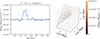 |
Fig. A.1. Relative difference of bispectrum estimate by our measurement code BiG and bskit for an example simulation. Left: For equilateral triangles, Right: for all triangle configurations |
Appendix B: Additional accuracy plots of the bispectrum correction model
This section shows two additional plots that illustrate the accuracy of BCM bispectrum emulator. While in Fig. B.1 we show the flattened and concatenated measurements from all three folding, we show in Fig. B.2 the same as a three-dimensional scatter plot.
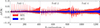 |
Fig. B.1. Accuracy of the emulator for baryonic effects on the matter bispectrum. The y-axis is defined as ΔR(k) = Remu/Rtrue − 1, where R(k) = BBCM(k)/BGrO(k). Here, we flattened and concatenated the three folding. The horizontal dashed lines show the 2% region. |
Appendix C: Parameter dependence
In this appendix, we explore further the dependences of two- and three-point statistics on both cosmological and baryonic parameters. We begin in the upper panel of Fig. C.1, with the dependence of the power spectrum ratio, S(k) = PHydro/PGrO, on baryonic feedback effects. In the lower panels of Figs. C.1 and C.2, we then show the dependence of bispectra ratio, R(k) = BHydro/BGrO for three different k configurations. Here we especially see that setting R(k1, k2, k3) = 1 if one ki < kmin might result in biased results.
In Figs. C.3 and C.4, we display the dependence of power spectrum and bispectrum on the BCM parameter θout and Minn. We apply the same baryonification, compatible with the FLAMINGO suite, to pairs of N-body simulations which vary one cosmological parameter at a time, in a wide range displayed in the legend. We note that, for simplicity, we use a simple linear interpolation and do not remove noisy measurements. However, this does not affect our conclusions. The dependence of θout and Minn is significantly smaller compared to other BCM parameters, such as M1 or β. Given their subdominant contribution, we decided to fix θout = 1 and Minn = 2.3 × 10¹³ h−1 M⊙.
Furthermore, we show in Fig. C.5 the dependence of S(k) and R(k) on cosmological parameters. To do so, we apply the baryonification with a fixed set of baryonic parameters to a set of N-body simulations, where one cosmological parameter at a time is varied. We find that, analogously to the results with the power spectrum obtained by Aricò et al. (2021a), Ωm and Ωb are the most significant, followed by σ8. The other parameters, including h, ns, Σmν, w0, wa, have a smaller impact than the nominal accuracy of the cosmological scaling, and thus we do not model them. Lastly, we show in Fig. C.6 the equivalent to Fig. 8 but for second-order statistics alone, and in Fig. C.7 the dependence of the three measured weak lensing statistics on the effects of baryonic feedback.
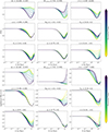 |
Fig. C.1. In this figure, we show the power spectrum’s dependence on baryonic feedback effects in the three upper rows. In the bottom three rows, we show the dependence of the bispectrum for k1 = k2 = k3. |
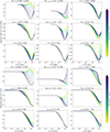 |
Fig. C.2. The same as the bottom three rows of Fig. C.1 but for two different settings of ki as indicated on the y-axis. |
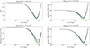 |
Fig. C.3. Dependence of the S(k) and R(k) on the BCM parameter θout. Yellow lines are smaller and blue lines are larger θout. |
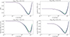 |
Fig. C.4. Dependence of the S(k) and R(k) on the BCM parameter Minn. Yellow lines are smaller and blue lines are larger Minn. |
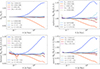 |
Fig. C.5. Dependence of the S(k) and R(k) on cosmological parameters. Here, we plot the ratio between each parameter’s lowest and largest values, as indicated in the legend. |
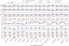 |
Fig. C.6. Same as Fig. 8 but second-order statistics alone. The triangles with error bars are estimated from the MCMC chains for all FLAMINGO models described in Sect. 2.2. Since the LS8 and Planck cosmology is different we plot ΔΩm = Ωmbest − Ωmtrue and in analogy ΔS8 and and ΔΩb. The different colours show cases where parameters are fixed. The stars indicate the best-fitting parameters resulting from a minimisation process that returns the lowest χ2. The corresponding figure for ξκ + ⟨ℳap2⟩+⟨ℳap3⟩ is shown in Fig. 8. |
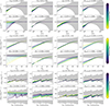 |
Fig. C.7. Dependence of the ⟨ℳapn⟩ and ξκ to changes of baryonic and cosmological parameters. We scaled the model vectors using the same model just for a GrO case, disentangling the effect of the baryons. The θap = {θap, 1, θap, 2, θap, 3} values for the lowest panel are increasing from left to right as in Fig. 4, increasing first θap, 3, then θap, 2 and lastly θap, 1. |
All Tables
Weighted average of the BCM best-fitting parameters over all FLAMINGO simulations considered in this work.
All Figures
|
Fig. 1. Accuracy of the emulator for baryonic effects on the matter power spectrum. The y-axis is defined as ΔS(k) = Semu/Strue − 1, where S(k) = PBCM(k)/PGrO(k). The horizontal dashed lines show the 0.5% region. |
| In the text | |
|
Fig. 2. Accuracy of the emulator for baryonic effects on the matter bispectrum R(k). The upper two rows show the lower and upper 68% percentiles of ΔR(k), and the two lower rows show the lower and upper 95% percentiles of ΔR(k). Each column is for a different k3 value, which is by construction larger than k2 and k1 but smaller than k1 + k2. The black circles show the actual location where we have measured B(k1, k2, k3). The background is coloured using a linear interpolation/extrapolation of the percentiles between the measured k-values. |
| In the text | |
|
Fig. 3. Baryonic effects on ⟨ℳap2⟩ (upper panel) and on ξκ (lower panel), illustrated by ratios of measurements with baryonic physics to GrO measurements. We show with blue triangles the fiducial FLAMINGO measurements, and the grey shaded area represents the Euclid DR1 uncertainty. We overplot with a red dashed line the best-fitting BCM to the flamingofied data vector, found by employing our emulators with fixed cosmological parameters. |
| In the text | |
|
Fig. 4. Same as Fig. 3 but for the ⟨ℳap3⟩ statistics. The x-axis shows different combinations of θap, 1-θap, 2-θap, 3. |
| In the text | |
|
Fig. 5. Posteriors of the cosmological parameters S8, Ωm, and Ωb, analysing a synthetic Euclid DR1 joint data vector of second- and third-order weak lensing statistics. We consider several cases. First, a gravity-only (GrO) data vector was analysed with a GrO model (purple contours). We obtain the black contours when baryonic effects are included in the data vector but not in the model. In orange, we illustrate the constraints we get when all elements of the data vector are excluded where the baryonic data vector deviates by more than 0.4σ from the GrO data vector. Lastly, we show the results if the model includes baryonic feedback in red and blue, where we fixed the baryon parameters to the truth in the blue case and marginalised over all five parameters for the red. The grey dashed line indicates the underlying D3A cosmology. |
| In the text | |
|
Fig. 6. Euclid DR1 forecast, where we used a flamingofied reference data vector (see Sect. 5.5) estimated from the fiducial baryon description of the FLAMINGO simulations with eight light cones of the 2.8 Gpc box. The stated constraints correspond to the joint analysis of second- and third-order statistics. The grey dashed line indicates the underlying D3A cosmology. |
| In the text | |
|
Fig. 7. Euclid DR1 forecast, where we used a flamingofied reference data vector (see Sect. 5.5) estimated from the fiducial baryon description of the FLAMINGO simulations with eight light cones of the 2.8 Gpc box. The stated constraints correspond to the joint analysis of second- and third-order statistics. The posteriors are the same as those used in Fig. 6, meaning we marginalised over all BCM parameters. The stated constraints correspond to the joint analysis of second- and third-order statistics (blue contours). The grey dashed line indicates the underlying D3A cosmology. |
| In the text | |
|
Fig. 8. Estimated weighted mean (triangles) and 68% credible intervals from the MCMC chains for all FLAMINGO models described in Sect. 2.2. Since the LS8 and Planck cosmology is different we plot ΔΩm = Ωmbest − Ωmtrue and in analogy ΔS8 and ΔΩb. The different colours show cases where parameters are fixed. The stars indicate the best-fitting parameters resulting from a minimisation process that returns the lowest χ2. The figure is for ξκ + ⟨ℳap2⟩+⟨ℳap3⟩. The corresponding figure for ξκ + ⟨ℳap2⟩ is shown in Fig. C.6. |
| In the text | |
|
Fig. A.1. Relative difference of bispectrum estimate by our measurement code BiG and bskit for an example simulation. Left: For equilateral triangles, Right: for all triangle configurations |
| In the text | |
|
Fig. B.1. Accuracy of the emulator for baryonic effects on the matter bispectrum. The y-axis is defined as ΔR(k) = Remu/Rtrue − 1, where R(k) = BBCM(k)/BGrO(k). Here, we flattened and concatenated the three folding. The horizontal dashed lines show the 2% region. |
| In the text | |
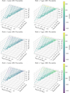 |
Fig. B.2. Similar to Fig. B.1, but now illustrated as a three dimensional scatter plot. |
| In the text | |
|
Fig. C.1. In this figure, we show the power spectrum’s dependence on baryonic feedback effects in the three upper rows. In the bottom three rows, we show the dependence of the bispectrum for k1 = k2 = k3. |
| In the text | |
|
Fig. C.2. The same as the bottom three rows of Fig. C.1 but for two different settings of ki as indicated on the y-axis. |
| In the text | |
|
Fig. C.3. Dependence of the S(k) and R(k) on the BCM parameter θout. Yellow lines are smaller and blue lines are larger θout. |
| In the text | |
|
Fig. C.4. Dependence of the S(k) and R(k) on the BCM parameter Minn. Yellow lines are smaller and blue lines are larger Minn. |
| In the text | |
|
Fig. C.5. Dependence of the S(k) and R(k) on cosmological parameters. Here, we plot the ratio between each parameter’s lowest and largest values, as indicated in the legend. |
| In the text | |
|
Fig. C.6. Same as Fig. 8 but second-order statistics alone. The triangles with error bars are estimated from the MCMC chains for all FLAMINGO models described in Sect. 2.2. Since the LS8 and Planck cosmology is different we plot ΔΩm = Ωmbest − Ωmtrue and in analogy ΔS8 and and ΔΩb. The different colours show cases where parameters are fixed. The stars indicate the best-fitting parameters resulting from a minimisation process that returns the lowest χ2. The corresponding figure for ξκ + ⟨ℳap2⟩+⟨ℳap3⟩ is shown in Fig. 8. |
| In the text | |
|
Fig. C.7. Dependence of the ⟨ℳapn⟩ and ξκ to changes of baryonic and cosmological parameters. We scaled the model vectors using the same model just for a GrO case, disentangling the effect of the baryons. The θap = {θap, 1, θap, 2, θap, 3} values for the lowest panel are increasing from left to right as in Fig. 4, increasing first θap, 3, then θap, 2 and lastly θap, 1. |
| In the text | |
Current usage metrics show cumulative count of Article Views (full-text article views including HTML views, PDF and ePub downloads, according to the available data) and Abstracts Views on Vision4Press platform.
Data correspond to usage on the plateform after 2015. The current usage metrics is available 48-96 hours after online publication and is updated daily on week days.
Initial download of the metrics may take a while.