| Issue |
A&A
Volume 705, January 2026
|
|
|---|---|---|
| Article Number | A176 | |
| Number of page(s) | 15 | |
| Section | Astrophysical processes | |
| DOI | https://doi.org/10.1051/0004-6361/202556100 | |
| Published online | 16 January 2026 | |
An XMM-Newton long look at the accretion disk plasma in the dipping neutron star LMXB 4U 1624–490
1
Anton Pannekoek Institute for Astronomy, University of Amsterdam Science Park 904 NL-1098 XH Amsterdam, The Netherlands
2
SRON Space Research Institute Netherlands Niels Bohrweg 4 NL-2333 CA Leiden, The Netherlands
3
ESO Karl-Schwarzschild-Strasse 2 D-85748 Garching bei München, Germany
★ Corresponding author: This email address is being protected from spambots. You need JavaScript enabled to view it.
Received:
25
June
2025
Accepted:
2
October
2025
Abstract
Context. Dipping neutron star low-mass X-ray binaries (NS LMXBs) are systems that exhibit periodic drops in their X-ray light curves. These are thought to be caused by material at the impact point of the gas stream onto the accretion disk, the bulge. Dipping systems are observed at high inclination and provide exceptional opportunities to address important open questions about accretion disks, such as the physical properties of the bulge, and the connection between disk atmospheres and disk winds.
Aims. We characterize the accretion disk plasmas in the 21-hour-period NS LMXB 4U 1624–490 and performed a detailed spectral analysis of the material in the impact region.
Methods. We used four XMM-Newton EPIC pn observations that specifically targeted dips and probed the dipping activity on different timescales (i.e., consecutive orbits and ∼6 months). We used a time- and flux-resolved spectroscopic analysis to probe the structural properties of the bulge moving along the line of sight and its homogeneity, respectively.
Results. During dipping, the primary spectrum is modulated by an ionized (log ξ ∼ 3.4) absorber with a varying column density and covering factor, and a colder absorber. This suggests that the bulge is a multiphase and clumpy absorbing medium. From size-scale arguments, we estimate the number of clumps in the bulge to be > 7 × 10³. A highly ionized disk atmosphere only becomes evident when different absorption phases are analyzed individually. We show that a physical picture of the bulge can be constructed, and we highlight that future research might reveal the dependence of its properties on the system parameters and determine whether the bulge might affect the dynamics of the accretion disk.
Key words: accretion, accretion disks / X-rays: binaries / X-rays: individuals: 4U 1624–490
© The Authors 2026
 Open Access article, published by EDP Sciences, under the terms of the Creative Commons Attribution License (https://creativecommons.org/licenses/by/4.0), which permits unrestricted use, distribution, and reproduction in any medium, provided the original work is properly cited.
This article is published in open access under the Subscribe to Open model. This email address is being protected from spambots. You need JavaScript enabled to view it. to support open access publication.
1. Introduction
Accretion of matter is a fundamental physical process that plays a role at various spatial scales in the Universe, from the formation of stars and planets to the evolution of binary star systems and galaxies. In low-mass X-ray binaries (LMXBs), the gas in the accretion disk is ionized by the strong X-ray emission from the region near the compact object. This leads to the formation of photoionized plasmas. These plasmas can be observed as static (e.g., disk atmospheres and coronae) or outflowing (e.g., disk winds) with a certain velocity (Begelman et al. 1983; Jimenez-Garate et al. 2002). These outflows carry away angular momentum and mass, with implications for the evolution of the accreting systems and their surrounding environment (e.g., Ponti et al. 2012; Justham & Schawinski 2012; Degenaar et al. 2014; Gallegos-Garcia et al. 2024).
The LMXBs that are observed at a high inclination are ideal laboratories for studying these accretion disk plasmas, which are detected through absorption lines from highly ionized elements in the X-ray spectra. Absorption from photoionized plasmas was first observed in the spectrum of the black hole LMXB GRO J1655–40 (Ueda et al. 1998). Since then, the powerful grating spectrographs on board of the X-ray Multi-Mirror Mission (XMM-Newton, den Herder et al. 2001) and the Chandra X-Ray Observatory (Chandra, Canizares et al. 2005), have significantly increased the number of detected absorbers and spectral features. To date, evidence for the presence of ionized absorbers has been found in a total of 33 LMXBs, 19 neutron star systems, and 14 black hole systems (Neilsen & Degenaar 2023). The properties of these spectral features yield information on the location and physical condition of the absorbing plasmas in the accretion disk environment (e.g., Xiang et al. 2009; Psaradaki et al. 2018; Trueba et al. 2020). Therefore, studies focused on ionized absorbers in high-inclination systems can help us to answer open questions related to accretion disk plasmas, such as understanding their geometry and location in the disk, or investigating how and if static and outflowing plasmas are connected with each other.
Evidence of high-inclination LMXBs are dipping and/or eclipsing phenomena (Frank et al. 1987). About two dozen dipping sources are known to date, and about half of them show eclipses (Avakyan et al. 2023). The dipping phenomena result from the interaction between the turbulent and dense stream of material from the companion star and the impact region of the accretion disk. The material that accumulates in the impact region periodically obscures the central X-ray source (White & Holt 1982; van Peet et al. 2009; Boirin et al. 2005; Díaz Trigo et al. 2006). These interactions can significantly increase the size of the accretion disk rim and generate a thick bulge (White & Mason 1985). Except for the debris left from the aftermath of the accretion stream impact that was reported for LMXB EXO 0748−676 by Psaradaki et al. (2018), the specifics of the structure and plasma properties of this impact bulge region of the accretion disk have not been extensively investigated so far.
The properties of the dips (e.g., duration, intensity, and substructures) vary significantly from one source to the next, and different models were proposed to explain the complex spectral changes observed between dipping and persistent (i.e., nondipping) spectra. Parmar et al. (1986) modeled the spectrum in terms of a persistent unabsorbed component with an associated absorbed component that was characterized by a varying degree of opacity. Church et al. (1997) explained the dipping with the partial and progressive covering of a point-like source emission by an extended absorber. Finally, Boirin et al. (2005) developed a third model that focused on ionized absorbers, were all observed spectral changes were modeled by variations in the properties of the ionized absorbers (e.g., column density and ionization). This model proved to be a viable interpretation for most of the known dipping sources (Díaz Trigo et al. 2006).
4U 1624–490, also known as the Big Dipper, is a bright – L(0.6 − 10 keV) ∼ 4.9 × 1037 erg s−1 (Xiang et al. 2009) – dipping neutron star LMXB and an excellent target for studying accretion disk and dipping plasmas. The orbital period of ∼21 h (Jones & Watson 1989) is the longest in dipping sources with regular dips. It causes a larger separation between the compact object and the companion star and a larger accretion disk radius (Smale et al. 2001) than in other dipping sources. In addition, the long dipping activity (∼3 h; Watson et al. 1985) makes the source ideal for the study of dips.
The source was first discovered by EXOSAT (Watson et al. 1985). The hydrogen column density in the line of sight of 4U 1624–490 is substantial (6 − 8 × 1022 cm−2), and the source was found to have a prominent scattering halo component (Angelini et al. 1997). Dust-scattering halos form when part of the source radiation is scattered by interstellar dust and is then directed back into the observer’s line of sight, with a certain delay. The response time of the scattering halo of 4U 1624–490 was estimated to be 1.6 ks (∼27 min; Xiang et al. 2007). The halo component was shown to be essential for modeling of the continuum, especially during dipping (Díaz Trigo et al. 2006).
The source lies at a distance of ∼15 kpc, which was calculated using the halo response time (Xiang et al. 2007). This is consistent with the value calculated by Christian & Swank (1997), who compared the hydrogen column densities derived from a spectral fitting to models of the exponential distribution of hydrogen in the Galaxy.
To date, the source has been studied using EXOSAT, XMM-Newton, and Chandra. The data from 1985 were first modeled with the complex continuum model (Church & Balucinska-Church 1995), and evidence of absorption of Fe XXV and Fe XXVI was then found in XMM-Newton data taken in 2001 (Parmar et al. 2002). These features were observed in persistent and dipping spectra, but were found to become shallower during the obscuration phase. This suggests that the absorber is less strongly ionized during dipping than in the persistent phase. The further analysis of the same dataset showed that all the spectral changes might be accounted for by a change in the properties of the ionized absorbers that during the dipping increased in column density and decreased in ionization (Díaz Trigo et al. 2006).
Chandra HETGS data taken in 2004 confirmed highly ionized iron and indicated two different plasmas in the accretion disk from which these lines originated: a hot corona, and a warm (i.e., less ionized) absorber located at the rim of the accretion disk (Xiang et al. 2009). Only an analysis of near dip events (Fig. 1 in Xiang et al. 2009) was included, however, and the dips were not analyzed.
We use unpublished XMM-Newton data and carry out the first detailed spectral analysis focused on the dipping behavior of the source, and a simultaneous analysis of dipping and persistent spectra. Specifically, we combined a time-resolved and flux-resolved analysis in order to characterize the accretion disk plasmas in 4U 1624–490 and understand the structure of the turbulent impact region of the accretion stream, the bulge.
2. Data analysis
The X-ray telescope on board the XMM-Newton space observatory (Jansen et al. 2001) is equipped with two X-ray instruments, the European Photon Imaging Camera (EPIC) and the Reflection Grating Spectrometer (RGS; den Herder et al. 2001). The EPIC has a total of three cameras with two different types of CCD, two MOS (Turner et al. 2001) and one pn (Strüder et al. 2001). The high-hydrogen column density in the line of sight of 4U 1624–490 causes strong absorption at lower energies, which means that no RGS data are available for the analysis.
Table 1 shows the log of the observations we used. All observations targeted the dipping phase of the source, and the corresponding light curves are shown in Fig. 1. This dataset allowed us to study the dipping phenomena on different timescales because Obs. 401 was taken ∼6 months after Obs. 301, while Obs. 401 to 601 belong to consecutive orbits. The observations were taken with the pn camera in timing mode, which is used to increase time resolution (up to 30 μs) and avoid pile-up in the data. With this observation mode, the data on the CCD are collapsed into a one-dimensional row along the y-axis. Spatial information is maintained only along the x-axis (RAWX), which indicates the pixels of the pn CCD chip. The data were retrieved from the XMM-Newton public archive, and all data products were extracted using the Science Analysis Software (SAS, v.21.0.0) and HEASOFT (v.6.32). We verified that the observations were not affected by background flares. To select a source and background region, we considered the distribution of photon counts over the CCD. For all observations, we defined the source region to be RAWX = [28−48] (Fig. 2).
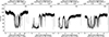 |
Fig. 1. Composite 0.3−10 keV light curves of the four EPIC pn observations with a binning in time of 5s. The light curves show persistent and dipping intervals. |
Observation log for the EPIC pn observations.
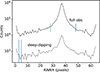 |
Fig. 2. Histogram of the total number of photons counts vs. RAWX for the original event file of the full observation (solid line) and for the event file from the deep-dipping time interval (dotted line). The defined source region RAWX = [28−48] and background region RAWX = [3−5] are indicated with vertical lines. The plot shows the background contamination by the source emission displayed by the difference in counts around the wings of the distributions. Data shown for Obs. 301. |
For timing-mode observations of bright sources, the edges of the CCD can still be significantly contaminated by the source emission and/or scattering halos1. For the background region, we initially selected RAWX = [3−5], but the background for all observations was highly contaminated with source emission. To minimize this effect, we selected the time interval that included the deepest of the dipping activity, which represents the period with the least radiation from the source, and therefore the least contaminated background, as shown in Fig. 2. Therefore, we selected the background region to be again RAWX = [3−5], but extracted from the deep-dipping interval event file (Fig. 2). We scaled this new background file to the correct exposure for each of the time intervals selected for the analysis (Sect. 3.1). This was done through the fakeit command in XSPEC v. 12.13.1 (Arnaud 1996). A simple absorbed power law was provided as input model to fakeit. This background extraction procedure was carried out for each observation individually (i.e., the background file was extracted from the deep dipping of each observation). Finally, we verified that the data were not affected by pile up using epatplot.
3. Spectral analysis and modeling
3.1. Light curves and time intervals
Dips are present in all observations, and a great variety of light-curve profiles are displayed (Fig. 1). Obs. 301 and 601 cover the start of the dipping activity, while the source was already dipping when Obs. 401 and 501 began. The bulk of the dipping and the post-dipping activity are sampled by all four observations. Using the ephemeris calculated by Smale et al. (2001), we phase-folded the data to investigate the recurrence and possible nature of the modulations. The 0.3−10 keV phase-folded light curves are shown in Fig. 3 with a time binning of 5s.
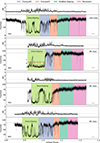 |
Fig. 3. Phase-folded light curves of all EPIC pn observations based on the ephemeris from Smale et al. (2001). Phase 0 is defined as the center of the dip. The uncertainty on the phase due to error propagation of the ephemeris is displayed as an error bar in the bottom right corner of each plot. All light curves are 0.3−10 keV and have a 5s time binning. In the top panel of each plot, the hardness ratios (5−10 keV/1.7−5 keV) for each observation are shown. The average persistent count rate is indicated as a dashed line in each light curve. The time intervals selected for the time-resolved analysis are shown for all observations: Clumps 1, clumps 2, shallow dipping, and persistent dipping (light blue, orange, dark green, and pink, respectively; see also Sect. 3.1). The duration of the deep-dipping interval is shown in all observations (light green). The intensity ranges for the flux-resolved analysis of the deep dipping in Obs. 401 are also indicated (a, b, and c); see Sect. 3.4. |
The quality of the datasets and the chosen time binning unveil types of modulations that seem to be recurrent. In all observations, it is possible to identify the bulk of the dipping coverage, followed by an irregular and gradual flux recovery as the bulge moves away from the line of sight. We classified the variety of modulations observed in the light curves as described below.
-
Deep dipping is the strongest obscuration due to dipping activity (Fig. 3). Throughout the observations, it displays a similar duration of ∼2 hours (around 10% of the orbital period). The obscuration shows a nonuniform coverage that allows the radiation to temporarily pass through. This results in an apparent W-shape in the light curve. The dipping activity occurs during the entire interval.
-
Clumps 1 are very short nearly fully absorbed intervals that recall sporadic clumps that pass through the line of sight (hence the name). During these intervals, the observed count rate drops to values that are very close to those of the deep dipping, but the observed modulation changes, namely its duration and shape. This is distinct from the deep dipping. The dipping activity is always at least > 1/2 of the interval duration.
-
Clumps 2. With these intervals, we sample the modulation where the flux recovery from the dipping is interspersed with a smaller sudden deep coverage that is shown by fast drops in the count rate. In this category, the dipping activity is ≤1/3 of the interval duration.
-
Shallow dipping are intervals in which we sample a gradual and constant flux recovery.
-
Persistent are intervals without modulation.
These selections are not merely based on a flux variation, as in previous studies (e.g., Díaz Trigo et al. 2006; Boirin et al. 2005), but are meant to indicate different time-varying structures that contribute to the obscuration. These types of modulations are identified in all observations, with only a few exceptions. For example, in Obs. 401 and 601, the gradual count-rate recovery during the shallow dipping is not as evident as in Obs. 301 and 501. The clumps 1 interval does not appear in Obs. 501. In Obs. 601, its seems as if the clumps 1 interval has doubled in duration (Fig. 3).
We used these intervals to perform a detailed time-resolved spectral analysis. We systematically investigated the spectral properties of the plasmas throughout the dipping phase and their evolution in time. The selected categories are also shown in Fig. 3. The deep dipping was excluded from the time-resolved analysis because it had various profiles and a level of contamination (i.e., different amounts of source radiation passing through the blocking medium) that precluded a systematic study throughout all observations. This is also shown by the hardness ratio (HR) diagrams (Fig. 3; for the HR we ignored data points below 1.7 keV as during the spectral fitting because of the high absorption). Spectral hardening was observed during dipping activity (Díaz Trigo et al. 2006; Boirin et al. 2005) and is clearly visible in the clumps 1 and clumps 2 intervals. During the deep-dipping intervals in all observations, the variations in the HR are quite complex and structured, however. This shows a combination of hardening and softening. To analyze the deep-dipping intervals, we therefore performed a flux-resolved analysis instead. We describe it in Sect. 3.4.
3.2. Baseline model
We performed the spectral analysis using SPEX version 3.08.01 (Kaastra et al. 1996). All data were optimally rebinned within SPEX obin. The uncertainties on the spectral fitting parameters were calculated with the error command and are reported as 1σ errors. This corresponds to a confidence level of 68%. We constructed a baseline model consisting of the accretion flow, the absorption components, and the scattering halo. The components of the continuum accretion flow are the disk (or neutron star boundary layer), the corona, and the fluorescent iron line from the disk reflection (see Fig. 4, components 1–3). These are described with a blackbody (bb), a power-law (pow), and a Gaussian (gaus) component, respectively.
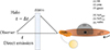 |
Fig. 4. Schematic of our spectral model. The sketch illustrates the direct source emission from a point in time t, and the halo-delayed source emission from the moment t − Δt. A legend for the model components (SPEX syntax) is also shown. |
The absorbing components that attenuate the accretion flow emission are the constant Galactic absorption and a time-varying absorption local to the system, caused by the movement of the bulge structure with the disk (see Fig. 4, components 4–6). Galactic absorption was modeled with a collisionally ionized absorber (hotgal). The time-varying local absorption has a cold and an ionized component (Díaz Trigo et al. 2006; Xiang et al. 2007, 2009), and we therefore used an additional cold component (hotloc) together with a photoionized absorber component (xabs).
To account for the expected scattering halo, we followed the model by Díaz Trigo et al. (2006). We first reduced the source emission (i.e., absorbed accretion flow emission) by a factor of e−τ(E) (etau model in SPEX), which corresponds to the scattering of photons out of the line of sight. The optical depth τ(E) was defined as  , where τ1 is the optical depth at 1 keV, and E−2 is the energy dependence for the dust-scattering cross section. Throughout the text, we refer to this first part of the model as “direct emission”. We then added a second part to our model in which the source emission was multiplied by a factor (1 − e−τ(E)), which accounts for the part of the halo photons that are scattered back into the line of sight (see Fig. 4). Similarly to the first part of the model, a hotgal and hotloc component were used for cold absorption from the ISM and local to the source, respectively. Limited by the data quality, no ionized absorption local to the source was included in the second part of the model. A sketch of our model is shown in Fig. 4, and our complete model in SPEX syntax is
etau*[hotgal*hotloc*xabs(bb+pow+gaus)]
+(1–etau)*[hotgal*hotloc*(bb+pow+gaus)]
Our aim was to investigate the time-variable absorbing components related to the bulge structure. Following the approach proposed by Boirin et al. (2005) and Díaz Trigo et al. (2006), we therefore kept the baseline model fixed and modeled all spectral changes during the dipping intervals by allowing the properties (i.e., column density and ionization) of the cold and ionized absorbing components in the accretion disk to vary. Specifically, all continuum parameters were coupled and the absorber properties were allowed to change throughout the time intervals. With this approach, we assumed that the accretion flow emission stays constant. Exceptions are reported in Appendix C. For each observation, we used the baseline model and fit all the spectra from the different time intervals simultaneously.
Further fitting details of the baseline model are as follows. First, the medium temperature was fixed to 10−6 keV to mimic a cold absorber for Galactic and local cold absorption. Second, the Galactic column density NH was fixed to 2.2 × 1022 cm−2 (HI4PI Collaboration 2016). Finally, for photoionized absorption, the column density NH and ionization level ξ were allowed to change. Xiang et al. (2009) reported an upper limit on the outflow velocity of the plasma (263 km/s). Because of the resolution of EPIC pn, we fixed the outflow velocity of the absorbers to zero.
Best-fit parameters and errors for the time-resolved spectral results. Obs. 601.
3.3. Time-resolved analysis. Simultaneous spectral fitting from clumps 1 through persistent
In this section, we report the spectral results of our time-resolved analysis, which was performed for all observations and included all time intervals defined in Sect. 3.1, except for the deep dipping. In the following, we use Obs. 601 to illustrate the main results of our time-resolved analysis and also discuss the general trends in the context of all the observations. Further details of the spectral results of Obs. 301, 401, and 501 are reported in Appendix A.
The spectral results of Obs. 601, including the model and residuals are shown in Fig. 5. Our model describes the spectra well, and the best-fit parameters are shown in Table 2. In the persistent interval, the continuum accretion flow emission is described by a power law with index Γ ∼ 1.9, a blackbody component with a temperature T of ∼1.5 keV, and a Gaussian emission feature centered at 6.5 keV. We fixed the full width at half maximum (FWHM) of the Gaussian feature to 0.23 keV, following Xiang et al. (2009). The spectra from the other intervals were coupled to these continuum parameters, and all spectral differences were modeled solely by changes in cold and ionized absorption. We list and discuss the results of the selected time intervals below.
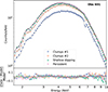 |
Fig. 5. Spectra from the selected time intervals of Obs. 601 with the same color-coding as in Fig. 3. The solid black lines represent the model for each spectrum, and the residuals are shown in the bottom panel. |
Clumps 1 and clumps 2 (i.e., progressively moving toward the outer edge of the bulge). Of the local time-varying absorption, the colder material (hotloc) has the highest NH value of ∼13 × 1022 cm−2 in the clumps 1 spectrum (i.e., closest to the deep dipping; Table 2). The column density then gradually starts to decrease from the clump#2 interval (i.e., as the bulge moves away from the line of sight). Ionized absorption (xabs) is detected in both intervals (Fig. 5, light blue and orange spectra, respectively). The absorbers have a similar ionization value log ξ ∼ 3.5, while the column density is higher by a factor ∼10 in clumps 1 than in clumps 2. This indicates a significant decrease in the amount of absorbing material going from the former to the latter interval.
In Fig. 6 we plot the properties (i.e., column density and ionization level) of the cold and ionized gas in clumps#1 and clumps#2 for all four observations. We note that the local cold absorption in clumps#1 and clumps#2 (Fig. 6, top panel) has column density values ( ) that are consistent through all observations.
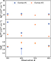 |
Fig. 6. Trends from the spectral results of the clump#1 and clump#2 intervals for all observations (301, 401, 501, and 01). No clumps#1 were identified for Obs. 501 (see Sect. 3.1). From top to bottom: Column density value of the local cold absorption ( |


In terms of ionized absorption (Fig. 6, middle panel), the column density value ( ) for clumps#1 varies slightly by up to a factor 3. For clumps#2, the results are consistent through Obs. 301, 401, and 601. The column density of the absorber is highest in Obs. 501, which might be explained by the additional slow and gradual attenuation of source emission on top of the sporadic clumps. This is displayed in the light curve (Fig. 3).
The ionization of the gas (Fig. 6, bottom panel) appears to always have a value log ξ ∼ 3.5, with some small variations between observations2.
Overall, the spectral results of clumps#1 and clumps#2 appear to be quite constant over time, which provides a picture of the evolution of the properties of the absorbing gas in the bulge over the timescales we sampled (i.e., 301 versus 601, ∼6 months, and 401 versus 601; consecutive orbits, i.e., 21 h). Our results show that the properties of the dipping plasmas do not seem to have changed over a timescale of months (Obs. 301 versus 601), although small changes are evident over consecutive orbits (401 versus 501 versus 601).
Shallow dipping and persistent. The local time-varying cold absorption (hotloc) follows a decreasing trend from clumps 1 to the persistent spectra. This trend is consistent throughout all observations. In the persistent interval, cold absorption local and Galactic always adds up to a column density value NH ∼ 10.7 × 1022 cm−2, which implies that a significant fraction is local to the source, as expected (Díaz Trigo et al. 2006; Xiang et al. 2007, 2009).
In the shallow-dipping and persistent intervals, the ionized absorber was not significantly detected (Fig. 5, green and pink spectra, respectively) when the spectra were simultaneously fit with the clumps 1 and clump#2 intervals. This was the case for all observations (Tables A.1, A.2, A.3 and 2), and it is supported by the HR diagram, which shows no changes between the two intervals (Fig. 3 top panels). Nonetheless, we performed a separate additional analysis of all the shallow-dipping and persistent intervals individually to further investigate the ionized absorbers (see Table B.1).
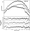 |
Fig. 7. Spectra from the selected intensity intervals for the deep dipping of Obs. 401. The spectra are labeled following the intervals shown in the second panel of Fig. 3. The solid black lines represent the model for each spectrum, and the residuals for each spectrum are shown in the bottom panels. |
Best-fit parameters and errors for the flux-resolved spectral results. Obs. 401.
3.4. Flux-resolved analysis. Deep-dipping spectrum results
We summarize the analysis and results of the deep dipping, that is, when the accretion emission was most heavily obscured. We also study the most impenetrable part of the bulge. As mentioned in Sect. 3.1, the deep-dipping intervals of the four observations showed that different amounts of source radiation passed through the blocking medium. A time-resolved analysis is hampered by this. Therefore, we opted for a different approach and performed a flux-resolved spectral analysis of one of the deep-dipping intervals. We selected the interval through which the least amount of source radiation passed, the deep-dipping interval of Obs. 401, and extracted spectra based on the dipping depth in the light curve. Specifically, a drop in the count rate of ∼80% (a), between ∼80% and ∼50% (b), and ≲50% (c) (Fig. 3). With the flux-cut analysis, we studied the parts of the bulge with maximum coverage such that almost all source emission was blocked (a) to parts through which the radiation passes sparsely (b) or almost completely (c). For these flux intervals, we describe their spectral results below.
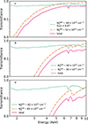 |
Fig. 8. Transmission plots (absorbed spectrum normalized by the continuum emission) for the direct emission of the flux-resolved spectra of the deep-dipping interval of Obs. 401 (a, b, and c). Each plot shows the transmission of the ionized absorber (xabs, dashed line), absorption from the total amount of cold material (dashed-dotted line), and the total transmission (solid line). All the absorption models were also convolved with the resolution of EPIC pn. The column density of the absorbers is indicated, together with the covering factor (fcov) values. If not indicated, the covering factor has a value of one. |
The spectral results of the three intensity intervals from the deep dipping of Obs. 401, including model and residuals, are shown in Fig. 7. Table 3 lists the corresponding best-fit parameters value. We used the same model and approach as in the time-resolved part of this work (i.e., we kept the continuum parameters coupled among the intervals and modeled any observed spectral changes with variations in the absorber properties).
Cold absorption appears to be highest in spectrum a with a value NH ∼ 82 × 1022 cm−2, which is almost a factor of 8 higher than in c and a factor of 2.5 higher than b. This intuitively suggests that the highest absorption from the blocking medium is sampled in a. Concerning the ionized absorption, we were able to fit one absorber in each of the three spectra. The column density is NH ∼ 82 × 1022 cm−2 in a, while it decreases to ∼60 × 1022 cm−2 and ∼48 × 1022 cm−2 in intervals b and c, respectively. We coupled log ξ for the three flux intervals, but set an upper limit to 3.45 (the value found in clumps 1, closest in time to the deep dipping: see Table A.2). This was done to avoid that unphysical values from the spectrum of interval a (with the lowest statistics) interfere with the fit because we found that the log ξ value pegged at the upper limit of any range given. We note, however, that in intervals b and c, the absorber is well constrained below the upper limit value when it is allowed to vary independently. The covering factor of the absorber is > 0.57 in a and b, and it is 0.87 for c.
These spectral changes in the column density and covering fraction values of the absorbing gas in the three intensity intervals of the deep dipping can be visualized with transmission plots. The transmission of each absorber was obtained by normalizing the absorbed spectrum by the continuum emission. In Fig. 8 we plot the transmission of all these gas phases (solid magenta line), the ionized gas (dashed light green line), and the cold intrinsic component (dashed-dotted orange line). The plots show that the reduction in column density of the ionized and the cold gas between spectrum b and c causes more radiation to pass through. This is also visible in the light curve, where interval c shows that a significant amount of the direct continuum is filtered through (Fig. 3).
3.5. Component of the scattering halo
We describe the complexities of the treatment of the halo component below. The halo model we used is described in Sect. 3.2. The halo column density varied throughout all intervals during the fit, as was done in Díaz Trigo et al. (2006), because our spectral analysis spanned intervals that exceed the halo-response time. Because the contribution of the scattering halo is strongest when the overall flux is low (i.e., deep dipping), however, the halo contribution is more difficult to constrain during intervals of still relatively high flux (i.e., clumps 1 through persistent). Some values were therefore forced to stay constant nonetheless.
Specifically, for each observation, the halo column density value was obtained from clumps 1 (i.e., the closest to the deep dipping), and it was then kept fixed for the other intervals (i.e., clumps 2, shallow dipping, and persistent) to avoid unphysical values. This was done because the time-resolved analysis (Sect. 3.3) did not include the deep-dipping intervals. For all observations, we found NH ∼ 10 × 1022 cm−2, which is also consistent with the value of cold absorption in the persistent direct part of the emission (Tables 5, A.1, A.2, and A.3). For the optical depth of the scattering halo, we allowed τ1 (defined in Sect. 3.2) to vary between 1.8 and 2.5 according to the values reported by Díaz Trigo et al. (2006) and Bałucińska-Church et al. (2000).
The halo component appears to be essential for modeling the flux-resolved spectra. As shown in Fig. 9, in the of three intensity intervals we sampled, the direct source emission (solid red line) and halo component (dotted blue line) contribute differently to the total flux. During the maximum coverage of the deep dipping (spectrum a), the direct part of the emission is highly attenuated by the high column density of the material that blocks the radiation. Most photons below 5 keV come from the scattered halo emission and cause the apparent bump at lower energies and the flattened shape. When the absorber column density decreases and some radiation can pass through the medium (spectrum b), this recovery of direct-source emission overpowers the halo contribution and causes the apparent flattening of the spectrum below 5 keV. At the moment of maximum flux recovery sampled during the deep dipping (spectrum c), the direct emission dominates the observed spectral shape so that it resembles the shapes shown in the time-resolved analysis.
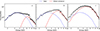 |
Fig. 9. Model components for the flux-resolved spectra of the deep-dipping interval of Obs. 401 (a, b, and c). We show that the direct and scattered emission (see Fig. 4) dominate for different flux levels. The direct part of the emission is shown in red (solid line), and the halo component is shown in blue (dotted line). The halo contribution in spectra b and a causes the double bumped/flattened shape. |
4. Discussion
We set out to investigate the properties of the dipping plasmas in the NS LMXB 4U 1624–490 by means of a time- and flux-resolved analysis of four EPIC pn XMM-Newton observations.
4.1. The nature of the dipping material
We combined the flux-resolved (deep-dipping intervals a, b, and c) and time-resolved (clumps#1 and clumps#2) results of Obs. 401 and attempt a description of the nature and structure of the material causing the dipping. These intervals had the same continuum parameters (see Tables 3 and A.2) and allowed us to compare changes in the absorber properties (i.e., column density and ionization parameter) relative to each interval.
The results of our flux-resolved analysis explain the deep-dipping modulations observed in the light curves and their corresponding spectral changes with varying column density of cold and ionized absorbers, and changes in covering factor of the ionized ones. The ionization parameter of the gas remains consistent throughout the flux-selected intervals of the deep-dipping (Table 3). These results suggest that the obscuring medium during the deep-dipping interval is characterized by a multiphase (i.e., composed of colder and ionized gas), nonuniform, and clumpy medium. This might imply that the intervals of maximum coverage (a) are caused by an accumulation of smaller clumps. The partial blocking of the radiation (b) or the full transmittance (c) is caused by this nonuniform nature of the medium.
Our time-resolved spectral analysis appears to be consistent with this line of reasoning. As the bulk of the bulge moves away from the line of sight, in the intervals of clumps#1 and clumps#2, we sample the remaining substructure of the dipping plasmas. More specifically, in clumps#1, the column density of ionized and cold absorbers is reduced by a factor of ∼8 compared to the deepest dipping activity (flux interval a). The ionization of the gas remains log ξ ∼ 3.4, which indicates that a single type of dipping plasma changes in the column density. This suggests that the modulation in clumps#1 might be the result of a smaller aggregation of clumps compared to the deep-dipping interval a. In clumps#2, the column densities are reduced even further, which is expected because the light curve only shows sporadic clumps that block the line of sight. In this time interval, log ξ ∼ 3.7, suggesting that the gas is more highly ionized than during clumps#1 and the deep-dipping flux-selected intervals. This is reasonable because a lower column density of the medium (i.e., fewer clumps) would allow more radiation to pass through and ionize the gas. Finally, when the dipping plasma moves completely out of the line of sight, no further clumps are eventually observed in the light curves (e.g., shallow-dipping and persistent intervals).
We showed that the results are consistent among the four observations. The picture of a multiphased and clumpy medium with a similar nature that changes in column density holds consistently for all our dipping datasets.
Finally, we produced some simple estimates of the physical sizes of the bulge and its clumps in relation to the system. The radius of the accretion disk was estimated to be ∼1.1 × 10⁶ km (by Church & Bałucińska-Church 2004, calculated from the Roche Lobe size of the neutron star). The deep-dipping interval lasts ∼2.1 hours (about 10% of the orbital period; Fig. 3). This results in a physical size of ∼6 × 10⁵ km along the circumference, assuming that the bulge region is located at the rim of the disk. When we assume that the bulge is an agglomeration of smaller clumps, we might interpret the modulations in clumps#2 as a unit scale for the clumps and perform a similar calculation. The light curves show that the modulation that resembles a single clump (Fig. 3, second panel, orange interval) occurs in a fraction of ∼5 × 10⁻⁴ of the orbital period, which corresponds to ∼38 s and a physical size of ∼940 km. This estimated value is comparable with the predicted value by Eq. (9) in Frank et al. (1987), which was obtained by assuming the neutron star mass to be 1 M⊙, the accretion stream half-width to be ∼109 cm, and the residual function f to be 6 (i.e., that 60% of the accretion rate remains in the residual stream).
We note that clumps that last shorter are also present, but they appear to be have a much lower column density and must therefore affect the obscuration due to the bulge less. The ratio of the two physical sizes (the bulge extension along the disk rim and the size of the single clump) gives ∼7 × 10³ as an estimate of the number of clumps that might make up the bulge. Our estimate is significantly lower than the predicted number of clumps at a given time according to Eq. (10) in Frank et al. (1987). This is expected because we only estimated the number of clumps in the bulge core region (i.e., deep dipping) and did not account for any of its outer layers or residual components (i.e., clumps#1 and clumps#2). Furthermore, our estimate likely represents a lower limit because we assumed that the entire obscuring structure lies at the edge of the disk, while some of it might likely extend to the inner regions of the disk (Frank et al. 1987).
4.2. An extended accretion disk atmosphere
Following our additional analysis (Appendix B), the persistent and shallow-dipping intervals show evidence for the possible presence of ionized gas with a column density NH ∼ 3 − 4 × 1022 cm−2 and NH ∼ 1 − 2 × 1022 cm−2 and an ionization log ξ ∼ 4.7 and log ξ ∼ 3.9, respectively (see Table B.1).
With regard to the persistent intervals, Xiang et al. (2009) detected an absorbing component with log ξ ∼ 4.3 in a Chandra observation in intervals close to and far from dipping (‘near dip’ and ‘far dip’ from Fig. 1 in Xiang et al. 2009). We found an ionized absorber consistent with the Chandra study during persistent intervals, but were unable to detect the ionized atmosphere during intervals of dipping or clumps, likely because the spectral resolution of our data is limited. In Sect. 4.1 we estimated the physical size of the unit clumps (i.e., modulations in clumps#2), and the accretion disk radius. Assuming our blackbody temperature is mostly representative of the disk, we estimated the disk scale height to be H ∼ 6 × 10⁶ km (assuming a neutron star mass of ∼1 M⊙). When we assume that the unit clumps are spherical, the size of the clumps is significantly smaller than the disk scale height. This implies the possibility of detecting two ionized absorbers, the atmosphere and the clumps.
For the shallow-dipping intervals, the fact that we are able to detect an ionized absorber regardless of whether the shallow modulation is evident from the light curves (Table B.1) might either indicate a type of modulation that is always present, but that we are not able to resolve, or some phase-dependent structure that is perhaps unrelated to any dipping activity.
In addition, it is insightful to compare our findings with the Chandra results, specifically, with the second absorber found in their far-dip intervals (Fig. 1 in Xiang et al. 2009). We note that some of these intervals agree in orbital phase with our clumps#1, clumps#2, and shallow dipping. The lower sensitivity of the Chandra light curves means that these modulations might not be resolved, and that they were consequently not included in the persistent analysis. Our results suggest that the second component found by Chandra (and also associated with the disk rim) might be the remaining substructure of the bulge, and it probably does not differ from the other absorber found in their near-dip intervals.
An ionized atmosphere with changing properties might also be suitable to explain the ionized gas in the shallow-dipping interval. Simultaneous different plasma states are to be expected (Díaz Trigo & Boirin 2016), and different ionization zones and density layers might therefore be present throughout the extended accretion disk atmosphere. The presence and nature of this absorber in the shallow-dipping remain unclear at this stage, but can be addressed in future work with data from higher-resolution spectra.
5. Summary and conclusions
We used a large XMM-Newton dataset that focused on the dips of 4U 1624–490 over different epochs to characterize the structure and nature of the gas at the impact point of the gas stream onto the accretion disk. We studied the details of the dipping activity systematically by classifying the variety of modulations in the light curves (see Fig. 3).
-
By combining a time-resolved and flux-resolved spectral analysis, we were able to determine different structures that contribute to the X-ray obscuration, and to obtain insight into the nature of the dipping plasmas.
-
The column density and covering factor of the absorber progressively decrease from the most to the least dense parts of the bulge, while the ionization remains constant. This indicates the presence of clumps. The analysis of the heaviest part of the dipping interval showed variations in the amount of radiation that passes through, which is proof of an inhomogeneous nature. The bulge therefore appears to be clumpy and nonuniform, and multiphase. It is composed of both cold and highly ionized material.
-
We made some simple estimates of the physical sizes of the bulge and its clumps. When the shortest clump modulation (clumps#2; Fig. 3) is taken as a unit scale, the deep-dipping modulation might be composed of at least ∼7 × 10³ of these clumps.
-
-
The additional analysis we carried out for the intervals where dipping modulation was not evident or absent led to an insightful analysis related to the accretion disk structure.
-
We consistently found a highly ionized atmosphere in all observations. The ionization of the gas agrees with the current literature value and previous studies. Although we were unable to resolve it, we estimated that with a higher spectral resolution, this component should also be detected during moments when the dipping is less prominent (e.g., clumps#1 and clumps#2). It currently remains unclear whether it would also be detected during the deepest dipping activity (i.e., deep-dipping).
-
The nature of the shallow-dipping modulation remains unconstrained.
-
-
With a systematic comparison of the spectral results throughout all observations, we were also able to gain insight into the evolution of these dipping plasmas over time.
-
The properties of the dipping plasmas of 4U 1624–490 appear not to change on the long timescale sampled by our data (∼6 months). They might be affected by possible turbulent mixing in the impact region on shorter timescales (in between consecutive orbits). Variability studies found that turbulence is not necessarily needed to explain the observed line width (Xiang et al. 2009), however. This might be further revisited with XRISM (Tashiro et al. 2020) data, which provide a higher resolution.
-
-
Finally, we note that the dust-scattering halo is essential in modeling the source spectrum during the most heavily obscured states (the lowest-count spectra, b and a in Fig. 7). This was also pointed out by Díaz Trigo et al. (2006). A full characterization in time of the halo was not possible with this XMM-Newton dataset.
To conclude, we highlighted that dipping light curves and their spectra are powerful tracers for changes in the column density and properties of the gas layers in the accretion disk environment of LMXBs. With the aim of further understanding what sets the bulge properties, future work might involve studying possible connections between the properties of the ionized gas in the disk and the binary system parameters (e.g., accretion rate, orbital period, and disk size). In addition, questions that remain open can be addressed with higher-resolution XRISM data.
XMM-Newton Calibration Technical Note, XMM-SOC-CAL-TN-0083.
Acknowledgments
This work was based on observations obtained with of XMM-Newton data, a European Space Agency (ESA) science mission with instruments and contributions directly funded by ESA Member States and the USA (NASA). The Space Research Organisation of the Netherlands is financially supported by NWO. The authors would like to thank O. Porth for insightful discussions.
References
- Angelini, L., Parmar, A., & White, N. 1997, ASP Conf. Ser., 121, 685 [NASA ADS] [Google Scholar]
- Arnaud, K. A. 1996, ASP Conf. Ser., 101, 17 [Google Scholar]
- Avakyan, A., Neumann, M., Zainab, A., et al. 2023, A&A, 675, A199 [NASA ADS] [CrossRef] [EDP Sciences] [Google Scholar]
- Bałucińska-Church, M., Humphrey, P. J., Church, M. J., & Parmar, A. N. 2000, A&A, 360, 583 [Google Scholar]
- Begelman, M. C., McKee, C. F., & Shields, G. A. 1983, ApJ, 271, 70 [CrossRef] [Google Scholar]
- Boirin, L., Méndez, M., Díaz Trigo, M., Parmar, A. N., & Kaastra, J. S. 2005, A&A, 436, 195 [NASA ADS] [CrossRef] [EDP Sciences] [Google Scholar]
- Canizares, C. R., Davis, J. E., Dewey, D., et al. 2005, PASP, 117, 1144 [NASA ADS] [CrossRef] [Google Scholar]
- Christian, D. J., & Swank, J. H. 1997, ApJS, 109, 177 [NASA ADS] [CrossRef] [Google Scholar]
- Church, M. J., & Balucinska-Church, M. 1995, A&A, 300, 441 [NASA ADS] [Google Scholar]
- Church, M. J., & Bałucińska-Church, M. 2004, MNRAS, 348, 955 [Google Scholar]
- Church, M. J., Dotani, T., Bałucińska-Church, M., et al. 1997, ApJ, 491, 388 [Google Scholar]
- Degenaar, N., Miller, J. M., Harrison, F. A., et al. 2014, ApJ, 796, L9 [Google Scholar]
- den Herder, J. W., Brinkman, A. C., Kahn, S. M., et al. 2001, A&A, 365, L7 [NASA ADS] [CrossRef] [EDP Sciences] [Google Scholar]
- Díaz Trigo, M., & Boirin, L. 2016, Astron. Nachr., 337, 368 [Google Scholar]
- Díaz Trigo, M., Parmar, A. N., Boirin, L., Méndez, M., & Kaastra, J. S. 2006, A&A, 445, 179 [NASA ADS] [CrossRef] [EDP Sciences] [Google Scholar]
- Frank, J., King, A. R., & Lasota, J. P. 1987, A&A, 178, 137 [NASA ADS] [Google Scholar]
- Gallegos-Garcia, M., Jacquemin-Ide, J., & Kalogera, V. 2024, ApJ, 973, 168 [NASA ADS] [CrossRef] [Google Scholar]
- Gnarini, A., Lynne Saade, M., Ursini, F., et al. 2024, A&A, 690, A230 [NASA ADS] [CrossRef] [EDP Sciences] [Google Scholar]
- HI4PI Collaboration (Ben Bekhti, N., et al.) 2016, A&A, 594, A116 [NASA ADS] [CrossRef] [EDP Sciences] [Google Scholar]
- Jansen, F., Lumb, D., Altieri, B., et al. 2001, A&A, 365, L1 [NASA ADS] [CrossRef] [EDP Sciences] [Google Scholar]
- Jimenez-Garate, M. A., Raymond, J. C., & Liedahl, D. A. 2002, ApJ, 581, 1297 [NASA ADS] [CrossRef] [Google Scholar]
- Jones, M. H., & Watson, M. G. 1989, ESA Spec. Publ., 1, 439 [NASA ADS] [Google Scholar]
- Justham, S., & Schawinski, K. 2012, MNRAS, 423, 1641 [NASA ADS] [CrossRef] [Google Scholar]
- Kaastra, J. S., Mewe, R., & Nieuwenhuijzen, H. 1996, UV and X-ray Spectroscopy of Astrophysical and Laboratory Plasmas, 411 [Google Scholar]
- Neilsen, J., & Degenaar, N. 2023, ArXiv e-prints [arXiv:2304.05412] [Google Scholar]
- Parmar, A. N., White, N. E., Giommi, P., & Gottwald, M. 1986, ApJ, 308, 199 [NASA ADS] [CrossRef] [Google Scholar]
- Parmar, A. N., Oosterbroek, T., Boirin, L., & Lumb, D. 2002, A&A, 386, 910 [NASA ADS] [CrossRef] [EDP Sciences] [Google Scholar]
- Ponti, G., Fender, R. P., Begelman, M. C., et al. 2012, MNRAS, 422, L11 [NASA ADS] [CrossRef] [Google Scholar]
- Psaradaki, I., Costantini, E., Mehdipour, M., & Díaz Trigo, M. 2018, A&A, 620, A129 [NASA ADS] [CrossRef] [EDP Sciences] [Google Scholar]
- Smale, A. P., Church, M. J., & Bałucińska-Church, M. 2001, ApJ, 550, 962 [NASA ADS] [CrossRef] [Google Scholar]
- Strüder, L., Briel, U., Dennerl, K., et al. 2001, A&A, 365, L18 [Google Scholar]
- Tashiro, M., Maejima, H., Toda, K., et al. 2020, SPIE Conf. Ser., 11444, 1144422 [Google Scholar]
- Trueba, N., Miller, J. M., Fabian, A. C., et al. 2020, ApJ, 899, L16 [Google Scholar]
- Turner, M. J. L., Abbey, A., Arnaud, M., et al. 2001, A&A, 365, L27 [CrossRef] [EDP Sciences] [Google Scholar]
- Ueda, Y., Inoue, H., Tanaka, Y., et al. 1998, ApJ, 492, 782 [NASA ADS] [CrossRef] [Google Scholar]
- van Peet, J. C. A., Costantini, E., Méndez, M., Paerels, F. B. S., & Cottam, J. 2009, A&A, 497, 805 [NASA ADS] [CrossRef] [EDP Sciences] [Google Scholar]
- Watson, M. G., Willingale, R., King, A. R., Grindlay, J. E., & Halpern, J. 1985, Space Sci. Rev., 40, 195 [NASA ADS] [CrossRef] [Google Scholar]
- White, N. E., & Holt, S. S. 1982, ApJ, 257, 318 [NASA ADS] [CrossRef] [Google Scholar]
- White, N. E., & Mason, K. O. 1985, Space Sci. Rev., 40, 167 [Google Scholar]
- Xiang, J., Lee, J. C., & Nowak, M. A. 2007, ApJ, 660, 1309 [Google Scholar]
- Xiang, J., Lee, J. C., Nowak, M. A., Wilms, J., & Schulz, N. S. 2009, ApJ, 701, 984 [NASA ADS] [CrossRef] [Google Scholar]
Appendix A: Spectral fitting results for Obs. 301, 401, and 501
Below we show the details of the spectral analysis of Obs. 301, 401, and 501, specifically their spectra and best fit spectral parameters.
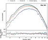 |
Fig. A.1. Spectra from the selected time intervals of Obs. 301 with the same color-coding as Fig. 3. Solid black lines represent the model for each spectrum, and residuals are shown in the bottom panel. |
Best-fit parameters and errors for the time-resolved spectral results: Obs. 301.
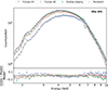 |
Fig. A.2. Spectra from the selected time intervals of Obs. 401 with the same color-coding as Fig. 3. Solid black lines represent the model for each spectrum, and residuals are shown in the bottom panel. |
Best-fit parameters and errors for the time-resolved spectral results: Obs. 401.
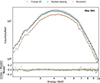 |
Fig. A.3. Spectra from the selected time intervals of Obs. 501 with the same color-coding as Fig. 3. Solid black lines represent the model for each spectrum, and residuals are shown in the bottom panel. |
Best-fit parameters and errors for the time-resolved spectral results: Obs. 501.
Appendix B: Additional analysis on persistent and shallow-dipping
Below we show the results of the additional analysis we carried out for persistent and shallow-dipping. For the persistent intervals, the aim was to investigate the presence of an ionized atmosphere in the disk. For the shallow-dipping, we wanted to investigate the properties of this modulation that seems to be the least consistent in all observations. Specifically, in Obs. 301 and 601 it appears as a gradual modulation of the continuum emission, while in Obs. 401 and 501 no evident modulation is present (Fig. 3).
Parameter values and errors for the additional analysis on persistent and shallow-dipping intervals of all four observations.
Appendix C: Note on continuum modeling
Here we describe some of the additional complexities of our baseline model and fitting.
As mentioned in Sect. 3.2, in our model we assume that the accretion flow emission stays constant throughout all intervals, however, this appears not to be the case for Obs. 301 and 401. In Obs. 301, the clumps 1 and clumps 2 spectra were fitted with a continuum independent from the persistent one (Table A.1). The changes in the best-fit values are a slight decrease in the black body normalization and an increase in the power law one (Table A.1). In Obs. 401, the same type of changes in continuum parameters are observed, the only difference being that the different continuum was needed for the shallow-dipping interval as well, in addition to clumps 1 and clumps 2 (Table A.2).
We notice that these changes in continuum parameters occur at different time intervals (i.e., likely being unrelated to any source “state” change, but rather linked to possible degeneracy in our model). Therefore we carefully tried to investigate these changes further.
Specifically, we first attempted to heavily rely on the continuum best fit values of the persistent interval from each observation, as we expect this to be where the continuum would physically dominate. Therefore, for both Obs. 301 and 401, we took the best fit values of each persistent interval, defined from these a range of ±15%, and fitted the other intervals by allowing their continuum parameters to vary within this range. This resulted in a worse fit with increased residuals (especially at energies > 8.5 keV and < 5 keV), and continuum parameters pegging at the lower/upper limit of the specified range. Finally, we also tried freeing the covering factor of the cold absorber, without any effect (i.e., covering factor remaining at a value of 1).
We believe that a possible explanation for these observed changes in continuum might be related to our current lack of understanding of the geometry of the corona for the source. Specifically, it might be the case that one of the two continuum components might be differently absorbed than the other one. For example, the emission from the disk and the region near the neutron star (black body component) might be covered completely by the bulge, but the corona might be more vertically extended (e.g., spreading layer geometry favored for the Comptonizing component in this source, see Gnarini et al. 2024). This implies that, during the different time intervals we sample, we might be seeing different amount of radiation from the corona being scattered (also given the high inclination of the system), which might result in different absorption for the two continuum components.
Finally, we note that the uncertainties in the modeling of the dust scattering halo (Sect. 3.5) for intervals where its contribution is not dominant (i.e., shallow-dipping and persistent) might also play a role in the changes in continuum. In addition, our current model does not account for scattered emission due to local cold material. Given the high column density values found (Sect. 3.3), we expect this component to make a contribution, especially during dipping intervals. The scattering due local material would be degenerate with the halo component (i.e., they will both contribute at lower energies), hence if there is something we are incorrectly accounting for about either one, this might have an effect on the best fit values of the continuum parameters as well (e.g., normalization of the power law component). However our conclusions about the global properties of the dipping medium should not be affected.
All Tables
Best-fit parameters and errors for the time-resolved spectral results. Obs. 601.
Best-fit parameters and errors for the flux-resolved spectral results. Obs. 401.
Best-fit parameters and errors for the time-resolved spectral results: Obs. 301.
Best-fit parameters and errors for the time-resolved spectral results: Obs. 401.
Best-fit parameters and errors for the time-resolved spectral results: Obs. 501.
Parameter values and errors for the additional analysis on persistent and shallow-dipping intervals of all four observations.
All Figures
|
Fig. 1. Composite 0.3−10 keV light curves of the four EPIC pn observations with a binning in time of 5s. The light curves show persistent and dipping intervals. |
| In the text | |
|
Fig. 2. Histogram of the total number of photons counts vs. RAWX for the original event file of the full observation (solid line) and for the event file from the deep-dipping time interval (dotted line). The defined source region RAWX = [28−48] and background region RAWX = [3−5] are indicated with vertical lines. The plot shows the background contamination by the source emission displayed by the difference in counts around the wings of the distributions. Data shown for Obs. 301. |
| In the text | |
|
Fig. 3. Phase-folded light curves of all EPIC pn observations based on the ephemeris from Smale et al. (2001). Phase 0 is defined as the center of the dip. The uncertainty on the phase due to error propagation of the ephemeris is displayed as an error bar in the bottom right corner of each plot. All light curves are 0.3−10 keV and have a 5s time binning. In the top panel of each plot, the hardness ratios (5−10 keV/1.7−5 keV) for each observation are shown. The average persistent count rate is indicated as a dashed line in each light curve. The time intervals selected for the time-resolved analysis are shown for all observations: Clumps 1, clumps 2, shallow dipping, and persistent dipping (light blue, orange, dark green, and pink, respectively; see also Sect. 3.1). The duration of the deep-dipping interval is shown in all observations (light green). The intensity ranges for the flux-resolved analysis of the deep dipping in Obs. 401 are also indicated (a, b, and c); see Sect. 3.4. |
| In the text | |
|
Fig. 4. Schematic of our spectral model. The sketch illustrates the direct source emission from a point in time t, and the halo-delayed source emission from the moment t − Δt. A legend for the model components (SPEX syntax) is also shown. |
| In the text | |
|
Fig. 5. Spectra from the selected time intervals of Obs. 601 with the same color-coding as in Fig. 3. The solid black lines represent the model for each spectrum, and the residuals are shown in the bottom panel. |
| In the text | |
|
Fig. 6. Trends from the spectral results of the clump#1 and clump#2 intervals for all observations (301, 401, 501, and 01). No clumps#1 were identified for Obs. 501 (see Sect. 3.1). From top to bottom: Column density value of the local cold absorption ( |
| In the text | |
|
Fig. 7. Spectra from the selected intensity intervals for the deep dipping of Obs. 401. The spectra are labeled following the intervals shown in the second panel of Fig. 3. The solid black lines represent the model for each spectrum, and the residuals for each spectrum are shown in the bottom panels. |
| In the text | |
|
Fig. 8. Transmission plots (absorbed spectrum normalized by the continuum emission) for the direct emission of the flux-resolved spectra of the deep-dipping interval of Obs. 401 (a, b, and c). Each plot shows the transmission of the ionized absorber (xabs, dashed line), absorption from the total amount of cold material (dashed-dotted line), and the total transmission (solid line). All the absorption models were also convolved with the resolution of EPIC pn. The column density of the absorbers is indicated, together with the covering factor (fcov) values. If not indicated, the covering factor has a value of one. |
| In the text | |
|
Fig. 9. Model components for the flux-resolved spectra of the deep-dipping interval of Obs. 401 (a, b, and c). We show that the direct and scattered emission (see Fig. 4) dominate for different flux levels. The direct part of the emission is shown in red (solid line), and the halo component is shown in blue (dotted line). The halo contribution in spectra b and a causes the double bumped/flattened shape. |
| In the text | |
|
Fig. A.1. Spectra from the selected time intervals of Obs. 301 with the same color-coding as Fig. 3. Solid black lines represent the model for each spectrum, and residuals are shown in the bottom panel. |
| In the text | |
|
Fig. A.2. Spectra from the selected time intervals of Obs. 401 with the same color-coding as Fig. 3. Solid black lines represent the model for each spectrum, and residuals are shown in the bottom panel. |
| In the text | |
|
Fig. A.3. Spectra from the selected time intervals of Obs. 501 with the same color-coding as Fig. 3. Solid black lines represent the model for each spectrum, and residuals are shown in the bottom panel. |
| In the text | |
Current usage metrics show cumulative count of Article Views (full-text article views including HTML views, PDF and ePub downloads, according to the available data) and Abstracts Views on Vision4Press platform.
Data correspond to usage on the plateform after 2015. The current usage metrics is available 48-96 hours after online publication and is updated daily on week days.
Initial download of the metrics may take a while.