| Issue |
A&A
Volume 705, January 2026
|
|
|---|---|---|
| Article Number | A93 | |
| Number of page(s) | 21 | |
| Section | Astronomical instrumentation | |
| DOI | https://doi.org/10.1051/0004-6361/202556210 | |
| Published online | 09 January 2026 | |
The CubeSpec space mission
II. Observational strategy validation
1
Institute of Astronomy, KU Leuven,
Celestijnenlaan 200D,
3001
Leuven,
Belgium
2
Leuven Gravity Institute, KU Leuven,
Celestijnenlaan 200D, box 2415,
3001
Leuven,
Belgium
3
ESTEC’ European Space Agency,
2200 AG
Noordwijk,
The Netherlands
4
School of Mathematical and Physical Sciences, Macquarie University,
Balaclava Road,
Sydney,
NSW
2109,
Australia
5
School of Mathematics, Statistics and Physics, Newcastle University,
Newcastle upon Tyne
NE1 7RU,
UK
★ Corresponding author: This email address is being protected from spambots. You need JavaScript enabled to view it.
Received:
1
July
2025
Accepted:
24
October
2025
Abstract
Context. Massive stars play a central role in astrophysics, yet their internal structure remains poorly constrained due to uncertainties regarding their core masses, internal rotation, and chemical mixing. Through pulsation mode identification, asteroseismology offers a unique window into stellar interiors. However, current spectroscopic ground-based observational campaigns suffer from diurnal and weather-induced gaps, and space missions historically assembled time series through photometry. A complementary strategy that delivers the necessary frequency resolution and high cadence is provided by spectroscopy, which is highly beneficial for unambiguous mode identification in β Cephei stars. CubeSpec is an ESA in-orbit demonstrator 12U CubeSat with a compact and high-resolution échelle spectrograph, dedicated to delivering space-based high-cadence high-resolution spectroscopy, which is used to identify mode geometries of β Cephei pulsators.
Aims. We investigated observational scenarios with various sampling pulsation cycles over the duration of the CubeSpec mission to ensure the retrievability of pulsation frequencies and unambiguously identify pulsation modes in massive stars, specifically from high-cadence high-resolution spectroscopic time series.
Methods. We simulated time series of line profile variations by combining atmosphere models with pulsation kernels. These synthetic time series include realistic instrumental responses, cadence variations, and noise characteristics. We assessed the retrievability of pulsation frequencies and mode geometries with two analysis techniques for different observational scenarios and various mode configurations, sampling cadence, mission time span, and data quality.
Results. Our simulations show that CubeSpec’s spectroscopic time series allow for reliable frequency extraction and mode identification across various pulsational and orbital scenarios, according to established science requirements of the mission. Especially, we identify mode amplitude and observational cadence as the key factors governing both the successful frequency retrieval and the critical conditions breaking it, thereby highlighting the need for modelling with a realistic cadence in the future.
Key words: asteroseismology / line: profiles / instrumentation: spectrographs / stars: early-type / stars: massive / stars: oscillations
© The Authors 2026
 Open Access article, published by EDP Sciences, under the terms of the Creative Commons Attribution License (https://creativecommons.org/licenses/by/4.0), which permits unrestricted use, distribution, and reproduction in any medium, provided the original work is properly cited.
This article is published in open access under the Subscribe to Open model. This email address is being protected from spambots. You need JavaScript enabled to view it. to support open access publication.
1 Introduction
Despite their importance, the evolution and the internal structure of massive stars both remain poorly constrained (Langer 2012). Large uncertainties remain regarding the physical processes at work beneath their stellar surfaces and evolutionary fundamental properties such as the (effective) mass of the convective cores and the effective length and form of mixing at the core boundaries and within radiative envelopes (Bowman 2020). The internal stratification of massive stars plays a key role in their evolution and lifetime, the type of end-of-life explosions they produce, and the nature of the compact objects left behind. It is therefore vital to constrain these physical processes given how they affect the astrophysical interpretation of gravitational waves (Abbott et al. 2016) and early-Universe observations (Wofford et al. 2012).
Asteroseismology provides a unique tool for probing the internal physics of stars by analysing their oscillation modes (Aerts et al. 2010). These pulsation modes are sensitive to internal conditions and can be detected through brightness variations thanks to photometric time series or spectral-line profile variations via spectroscopy. Among massive stars, β Cephei pulsators are particularly valuable targets for asteroseismic studies due to their well-defined pulsation frequencies and status as progenitors of core-collapse supernovae (Bowman 2020; Burssens et al. 2023). While a few of the brightest β Cephei stars have been extensively studied, unambiguous mode identification for many others remains a significant challenge.
Ground-based asteroseismology suffers from time gaps due to diurnal cycles and weather conditions, which often results in a complex spectral window and introduces aliasing, thereby complicating mode identification for asteroseismic modelling. Space-based photometry from missions such as Kepler/K2, CoRot, and TESS (Borucki et al. 2010; Auvergne et al. 2009; Ricker et al. 2015) has improved this situation significantly, leading to unambiguous identifications of many high-mass pulsators (Degroote et al. 2009; Blomme et al. 2011; Bowman et al. 2019a,b; Burssens et al. 2020). Yet, unambiguous mode identification has remained the main bottleneck in the detailed asteroseismic characterisation of massive stars (Bowman 2023). Spectroscopy offers a complementary path to mode identification by exploiting line profile variations caused by pulsation-induced velocity fields and temperature fluctuations. Techniques such as the moment method (MM; Briquet & Aerts 2003) and the Fourier parameter fit (FPF) method (Zima 2006) have proven successful in past ground-based studies. However, spectroscopic asteroseismology of massive stars has been limited to small samples due to sparse and interrupted time coverage (Aerts et al. 1995; Aerts & De Cat 2003; Aerts et al. 2003).
The CubeSpec mission (Raskin et al. 2018; Vandenbussche et al. 2021) is a forthcoming space-based high-resolution optical spectroscopic mission designed to overcome the limitations of sparse sampling common in ground-based datasets. CubeSpec is a European Space Agency (ESA) in-orbit demonstrator 12U CubeSat. It features a novel optical design, based on a compact telescope and échelle spectrograph, and delivers both high throughput and spectral resolving power (Raskin et al. 2018). CubeSpec will provide continuous, high-cadence spectroscopic monitoring of bright stars, enabling asteroseismic studies from space. This mission aims at delivering robust mode identification through high-resolution spectroscopy, opening the door to full asteroseismic modelling of β Cep stars, whose sample and science requirements for the demonstration mission are provided in Bowman et al. (2022). In preparation of CubeSpec’s expected launch in 2026, the observational strategy of the mission must be validated in order to ensure the feasibility of unambiguous mode identification. This was achieved using simulated data that replicate the expected instrumental setup and sampling, analysed with different techniques and under several mission conditions.
In this paper, we demonstrate the proof of concept of pulsation mode retrieval from mock observations that replicate the expected data quality of CubeSpec. In Sect. 2, we generate artificial time series of line profiles by combining a TLUSTY atmospheric model with FAMIAS-generated pulsation profiles, and we present and discuss the noise budget affecting our simulations. In Sect. 3, we define the various test cases, varying mode configurations, amplitudes, and in-orbit sampling scenarios to assess the frequency and pulsation mode retrievability of our synthetic data. Section 4 focuses on the how the time series are analysed with FAMIAS. The results are presented and discussed in Sect. 5, and we conclude in Sect. 6.
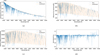 |
Fig. 1 (a) TLUSTY model atmosphere with Teff = 27 000 K, log g = 4.0, Vt = 2 km s−1, and Z = Z⊙ over the CubeSpec spectral range scaled to Vmag = 4. We show the astrophysical flux (blue) and corresponding continuum (orange). (b) Effective flux from Eq. (5) (blue) and corresponding continuum (orange). (c) Detector counts per pixel from Eq. (6) (blue) and corresponding continuum (orange). (d) Normalised spectrum. |
2 Spectral time series simulator
To simulate realistic observations made by CubeSpec, we developed a simulator that includes both the astrophysical simulation of the line profile variations (LPVs) integrated over the stellar surface and the instrument throughput and noise characteristics. We combined two principal open access tools. In Sect. 2.1, we present a TLUSTY stellar atmosphere model (Hubeny 1988). It contains metal line-blanketed, non-local thermodynamic equilibrium, plane-parallel, hydrostatic model atmospheres representative of the basic parameters appropriate to B-type stars. This static spectral structure is combined with pulsation profiles. We adopted the parameters of β Cep itself as a typical example of the class in order to design those pulsations. In Sect. 2.2, we describe how we used FAMIAS (Zima 2008) to generate the pulsation profiles. The individual processing of both tool inputs and how they are combined to design synthetic CubeSpec observations are discussed afterwards. In Sect. 2.3, we compute the noise budget resulting from the various contributors impacting the signal. Finally, in Sect. 2.4 we present target visibilities used for scheduling observations in of our time series.
2.1 CubeSpec 1D spectral simulator
We used the non-local thermodynamic equilibrium atmosphere code TLUSTY (Lanz & Hubeny 2007; Hubeny & Lanz 2017) to compute the astrophysical flux F(λ) of a prototypical Vmag = 4 B-type star (Fig. 1a). We adopted a model for Teff = 27 000 K, log g = 4.0, Vt = 2 km s−1, and Z = Z⊙ as our reference fiducial star as these parameters are close to those of β Cep itself (Catanzaro & Leone 2008). We include the instrumental characteristics of CubeSpec to estimate the number of photons reaching the detector. This was done by applying the optical response of the CubeSpec system to the spectral density flux of our fiducial Vmag = 4 β Cep star.
We re-binned the spectrum onto a wavelength grid defined by the geometric transformation from spectrograph slit to the pixel-sampled resolution element (slit image) on the spectrograph’s detector. This geometric transformation is in the form of an affine matrix that describes the translation, rotation, scale, and shear of the slit image for each wavelength and diffraction order. The transformation was retrieved from the Zemax optical design file of the spectrograph via a PyEchelle (formerly Echelle++; Stürmer et al. 2019) model. This provides the spectral coverage per pixel δ(λ). This transform varies as a function of wavelength along each order, as well as between orders. The spectral orders are available in Table A.1.
To express the flux in terms of photon counts, each flux element was divided by the photon energy at the corresponding wavelength. This photon-domain flux was then multiplied by the full instrument response, Rins(λ), which is composed of the optical system transmission, T(λ), and the detector quantum efficiency, QE(λ), to compute the effective flux measured by the instrument. We first defined the optical transmission, which describes the throughput of the optics:
 (1)
(1)
with Rmirror(λ) the mirror reflectivity, nmirror the number of mirror reflections, τD the efficiency of the grating, η2CD the transmission of the prism in double-pass, and BF(λ) the blaze function of the grating. The blaze function describes the relative diffraction efficiency across spectral orders, with a maximal efficiency at the centre (or blaze) of an order and a reduced efficiency at its edges. It is given by Schroeder (2000):
 (2)
(2)
where m is the spectral order number and λc its central wavelength (listed in Table A.1). T(λ) and BF(λ) are displayed in Figs. A.1a and A.1b, respectively. By multiplying the optical throughput by the detector’s quantum efficiency, we obtained the instrument response:
 (3)
(3)
We also defined the effective aperture (Aeff) as
 (4)
(4)
with A the aperture area of the primary mirror, Ob the obscuration due to the secondary mirror and Pjit the pointing jitter loss.
By combining previous equations, we obtained the effective photon flux received at the detector Feff(λ), shown in Fig. 1b, which relates to the astrophysical flux F(λ) as
 (5)
(5)
where Eph(λ) is the photon energy and RFGS is the flux loss for the fine guidance sensor. The parameter numerical values from the previous equations are provided in Table 1. We used the values of mirror reflectivity and quantum efficiency in the photometric bands (U, B, V, R, and I) to perform quadratic interpolations over the full wavelength range as displayed in Figs. A.1c and d. Also, we neglected here the field flattening element placed before the detector, and with a throughput superior to 98%, and consider a unitary detector gain. Finally, we computed the photon counts per pixel by integrating over each pixel’s wavelength coverage and exposure time (texp):
 (6)
(6)
The resulting signal S (λ) represents the number of photons detected per pixelised wavelength bin, and is shown in Fig. 1c. These steps are also applied to the TLUSTY continuum spectrum for future normalisation.
Numerical values of the instrumental parameters discussed in the main text, used for scaling the TLUSTY spectrum before convolution, noise, and stray light computation.
2.2 FAMIAS pulsation profiles
FAMIAS is a state-of-the-art software for asteroseismic analysis of photometric and spectroscopic time series data (Zima 2008). The software incorporates two main sets of tools. The first one focuses on searching for pulsation frequencies in the data by combining Fourier analysis with non-linear least-squares fitting algorithms. The other deals with pulsation mode identification from the detected frequencies. In addition, FAMIAS includes line profile synthesis to simulate time-dependent line profile variations imposed by stellar pulsation on the atmospheric spectrum of the pulsating star. Our simulations use user-defined stellar parameters, pulsation mode characteristics, broadening mechanisms, and time span. We made use of this module to generate time series of pulsation kernels in velocity space, to be convolved with the TLUSTY spectrum for simulating spectroscopic LPVs. Our simulations incorporate instrumental broadening by matching the intrinsic line width of pulsation profiles with CubeSpec’s average resolving power at the blaze (wintr = c/R = 5.45 km s−1), relying on FAMIAS assumption of a Gaussian intrinsic line profile. For rotational broadening, we worked with υe sin i = 100 km s−1 except in a test we conducted to investigate the lower rotational regime, for which we used υe sini = 10 km s−1. The time series are generated over a time span of 90 or 30 d, with a sampling of either 90 or 1 min, depending on the observational scenario (see Sect. 3.3).
We normalised the output of FAMIAS by the average equivalent width to ensure the conservation of the average equivalent width of spectral lines when later convolving with pulsation broadening profiles. Without it, artificial variations in the equivalent width could arise, misrepresenting the true effects of pulsations. Given that the equivalent width represents the total flux absorbed by a spectral line, it should remain on average constant in the absence of changes in the stellar fundamental properties. Since pulsations redistribute flux across the profile rather than altering the total absorbed flux, the equivalent width should remain unchanged on average. The synthetic CubeSpec’s spectra are then convolved with the times series of FAMIAS pulsation kernels, providing a time series of stellar spectra showing LPVs caused by pulsations.
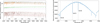 |
Fig. 2 Left: noise budget contributors: total (blue), shot (orange), stray light (green), readout (red), dark current (purple), and pixel gain variability (brown). Right: portion of the simulated, not convolved, spectrum after the addition of the noise. The focus is on spectral order 84, which contains the Si III triplet around λ4553, λ4567, and λ4574 lines and is used for asteroseismic diagnosis. |
2.3 Noise budget
The spectra obtained from convolutions account for a noiseless photon signal. During an observation, the stellar signal captured by the telescope and recorded by the detector is inherently impacted by statistical errors contributing to the noise budget of the measurement. To realistically assess this noise, we included these contributions in our simulations. These noise contributions are considered independent from one another. Therefore, the variance σ2(λ) of the measured 1D signal corresponds to the individual variances summed in quadrature (Bradt 2003):
 (7)
(7)
The first noise source, σS (λ) = S1/2(λ), is the shot noise of the detector signal. The stray light error contribution, σL(λ), accounts for the unwanted light fraction undergoing scattering or reflection within the instrument. The stray light variance is defined by its signal: σ2L(λ) = L(λ), which includes three components:
 (8)
(8)
which respectively express the scattering from the primary mirror M1, the reflection from the baffle, and the spectrograph internal component of stray light:
 (9a)
(9a)
 (9b)
(9b)
 (9c)
(9c)
where the γ factor in each equation respectively represents the number of photons scattered from M1, reflected by the baffle, and the fraction of local flux. We note that in our simulations we considered the stray light contribution from the star only and ignored stray light contributions (due to the Earth limb and the Moon). The number of pixels per spectral resolution element Npix/bin(λ) is obtained similarly to δλ(λ). The numerical values for the stray light parameters are given in Table 1. The remaining error contributions are associated with the readout of the detector, σRN, the shot noise on the dark current, σD, arising from the random thermal generation of electrons in the detector, and the inter-pixel relative gain variability, σG(λ). In the case of the readout and dark current noises, we accounted for the contribution of each of the n pixels spanning a resolution element on the detector in the cross-dispersion direction. By using the definition of each noise source, the variance of the measured 1D signal can be written as
 (10)
(10)
where RN is the read noise coefficient, D is the dark current rate and GV the relative inter-pixel gain variability. The numerical values for these parameters are provided in Table 1.
For each spectrum in our time series, we added a separate realisation of the noise of Eq. (6). We assessed the signal-tonoise ratio (S/N) of our data and obtain a peak S/N per pixel of 150, and a median S/N per pixel of approximately 125. These correspond to S/N per resolution element of 263 and 220, respectively, accounting for an average of 3.08 pixels per resolution element. The synthetic S/N spectrum for the current parameters Vmag = 4 and texp = 15 min is available in Fig. A.2. We show the various noise error contributors as well as a section of the spectrum after adding noise in Fig. 2, and an example of synthetic data in Fig. 3.
Our model features all the factors affecting the spectrum between the stellar emission and measurement on the detector. These include magnitude scaling, pulsations, noise distribution, and expresses the signal in terms of photons per pixel.
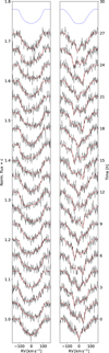 |
Fig. 3 Si III λ4574 line time series assuming an inclination of 60°, a projected rotational velocity (υe sin i) of 100 km s−1, a cadence of 90 min, and an exposure time (texp) of 15 min at Vmag = 4, resulting in a S/N of ≈ 140. Left panel: multimode configuration: a radial mode at 5.25 d−1 with an intrinsic velocity amplitude (υamp1) of 21 km s−1 and a sectoral l = m = 2 mode at 5.385 d−1 with υamp2 = 21 km s−1. Right panel: single mode configuration: a tesseral (l, m) = (8,6) mode at 5.25 d−1 and with υamp = 21 km s−1. The dashed red lines show the noiseless profiles, and the blue lines show the average profile of each series. |
2.4 Target visibilities
Sampling cadence and visibility constraints can significantly influence data quality and therefore analysis potential. A key aspect of the mission is the observational scheduling once the satellite is in orbit. Real observations will be affected by orbital constraints and evolving stellar visibility windows, inducing irregularities in the sampling. We simulated these effects in our time series under various scenarios to assess their impact on frequency retrievability.
To compute the target visibilities, we started by simulating the orbit in a commercial software. From there, we exported the direction vectors from the spacecraft to the Earth, the Sun, and the Moon, using a 1 min time step. We could then easily verify whether the angular distance between those objects and the optical axis pointing to any given target is compatible with the avoidance angles imposed by the spacecraft’s structure.
To avoid excessive stray light, avoidance angles of 90°, 20°, and 20° are imposed around the Sun, Earth, and Moon, respectively. A maximum angular distance of 45° is also imposed between the secondary spacecraft’s axis (Y) and the nadir, to prevent direct solar insulation on the radiators located on the -Y spacecraft panel (dissipating heat generated by the on-board electronics and the payload’s science detector). A sketch of the resulting constraints and results in visibility can be found in Fig. 4.
To have more flexible scenarios, we used the visibility windows computed for the high-priority target τ Lib in our simulations (see Bowman et al. 2022), as those combined the existence of two windows per orbit with the presence of visibility gaps imposed by the Moon. We further explore these two features in Sect. 3.4.
3 Observational scenarios
3.1 Pulsation model
To calibrate our synthetic data with a realistic representation of β Cephei pulsations, we modelled the pulsation behaviour of Alfirk (β Cep), the prototype of the β Cephei class. We combined a radial mode at f1 = 5.25 d−1 with a sectoral mode (l, m) = (2,2) at f2 = 5.385 d−1, and a 60° stellar inclination following the ground-based high-resolution spectroscopic study of Aerts et al. (1994).
3.2 Diagnostic lines
We performed the analysis with the Si III triplet visible in Fig. 2. The silicon triplet stands as key spectroscopic diagnostic due to its sensitivity to stellar pulsations, its strength, and the fact that it is temperature-broadening-dominated and, in slow rotators, not affected by blending (Mazumdar et al. 2006; Aerts & De Cat 2003; Bowman et al. 2022). We focused on the λ4567 and λ4574 lines because they are stronger and located at the blaze of the spectral order and, thus, benefit from a higher S/N. We note, however, that the λ4553 and He I lines are also good candidates (see e.g. Balona et al. 1999), despite the latter not matching the Gaussian shape approximation made in FAMIAS due to a Voigt profile caused by the combination of stark and rotation-dominated broadening mechanisms.
We define below a number of scenarios (SC1-SC11). These different scenarios test various mode configurations (Sect. 3.3), sampling effects (Sect. 3.4), and data quality (Sect. 3.5).
3.3 Mode configurations: Number of modes and amplitudes
To ensure realistic observational constraints and produce realistic observational campaigns, we began by validating frequency and mode retrievability with scenarios involving different configurations of pulsation modes and amplitudes. The simulation baseline for our time series implements a 60° inclination, υe sin i = 100 km s−1, a time span of 90 d, which is a pessimistic case of the shortest nominal mission duration, and a regular sampling with a 90 min cadence as an approximate orbital period.
SC1 RADIAL. We first included a single radial mode at 5.25 d−1 and with an intrinsic velocity amplitude of 21 km s−1.
SC2 TESSERAL. While space-based photometry favours the detection of low-angular-degree modes due to the geometric cancellation effect (Aerts et al. 2010), high-resolution spectroscopy allows higher-angular-degree pulsation modes to be detected since they contribute differently to LPVs. Therefore, we progressed to a more complex geometry by including a single tesseral mode with (l, m) = (8,6), with same frequency and amplitude as the previous radial mode, to represent a highangular degree modes and validate mode identification in such a scenario.
SC3 MULTI-EQ. We further simulated a multimode target by including the two pulsation modes described in Sect. 3.1. Difficulties in multimode identification may arise either from the presence of several modes or from a second mode with a lower amplitude. To disentangle these effects, we first examined simultaneous detection when both signals are equally strong. Here, the radial and sectoral mode (l, m) = (2, 2) are both injected with an intrinsic velocity amplitude of 21 km s−1.
SC4 MULTI-LOW. To complement the previous test, we kept the multimode configuration but reduced the amplitude of the sectoral mode to 3kms−1 to test sensitivity limits to detecting weaker pulsation signatures. The combination with the previous test allowed us to determine whether the challenge of multimode identification was intrinsic to multimode interaction or the detectability of low-amplitude signals.
SC5 SLOW-ROT. With the same configuration, we investigated the impact of rotational velocity on mode identification by reducing υe sin i to 10 km s−1.
SC6 AMP-THRESH. To explore detection thresholds, we systematically varied the intrinsic velocity amplitude in a single mode configuration and examine the resulting Fourier peak detection and significance for different mode geometries. This allows us to characterise the minimum detectable signal under CubeSpec’s expected conditions.
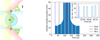 |
Fig. 4 Left: avoidance angles for CubeSpec. The grey shaded spacecraft is displayed at three positions along its orbit, assuming the optical axis is pointing in the anti-Sun direction. The green shades illustrate the regions of the sky accessible from each of those locations. The Moon is seen partly obstructing one of those regions. The zones of avoidance imposed by the Sun, the Earth, and CubeSpec’s radiator are shown in yellow, blue, and red, respectively. Right: simulated evolution of visibility window duration over 6 months of visibility of the star τ Lib, involving lunar interruptions. The vertical lines show the start (blue) of the observational campaign and the ends of 90 d (red) and 30 d (black) observational campaigns defined for the observing scenarios described in the main text (Sect. 3). The inset panel zooms into the start of visibility to highlight visibility windows. |
3.4 Sampling effects: Visibility, cadence, and the Moon
In all scenarios considered so far, we assumed time series to have a 90 min cadence, acquiring one observation per orbit at a fixed orbital phase. We now describe scenarios taking realistic orbits and visibilities into account.
For these scenarios, we considered the multimode configuration from SC4 MULTI-LOW and generate time series over 90d with a sampling of 1 min, using the strongest Si III line. Finally, we selected as observations the steps based on the constraints from the observational scenario and the actual visibility of the target. Here, we accounted for visibility gaps due to the Moon and excluded the corresponding periods from the time series, as a worst case scenario. Altogether, these conditions impact sampling uniformity, cause data loss and can introduce aliasing effects potentially affecting frequency retrievability.
SC7 RAND-VIS. In this scenario we randomised the time at which each observation is made within its orbit, while ensuring stellar visibility and maintaining data quality.
SC8 BOOST-CAD. We investigated the impact of sampling the pulsation cycles on frequency retrieval by increasing the observing cadence. To improve cadence, we accounted for the dynamics of the visibility windows, initially appearing as two separate segments per orbit then gradually merging into a single longer window. We defined the observability window as spanning the visibility window excluding its final 15 min, ensuring sufficient time for a full exposure. Observations were scheduled as follows: (1) for visibility windows shorter than 15 min, a single observation was made at the start; (2) for 15-30 min long, one observation was randomly scheduled within the observability window; (3) for windows longer than 30 min, two observations were scheduled randomly in the observability window, with at least a 15 min gap between exposures to accommodate integration time. This roughly doubled the cadence while preserving data quality.
Comparison of the different observational scenarios.
3.5 Data quality
In addition to sampling, data quality is an important factor influencing frequency retrievability. To investigate this, we explored various S/N conditions and/or more pessimistic mission scenarios in terms of campaign duration to determine the boundary limits for a successful retrieval of the frequency.
SC9 ADAPT-S/N. We scheduled one observation at the start of each visibility window and varied the exposure time according to their duration. For short windows, the exposure time was reduced to match the window duration, while we maintained the nominal exposure time for longer windows. The noise models were recalculated accordingly to the integration time.
SC10 SHORT-FULL. We first degraded the duration of the mission and simulated a shorter campaign of 30 d while maintaining the quality of the data and taking one random observation per orbit.
SC11 SHORT-HALF. Finally, we combined degraded data and degraded observational campaign lengths to explore CubeSpec’s robustness to more drastic mission conditions. In addition to a shorter campaign, we also reduced the S/N by half, still with one random observation per orbit.
This structured exploration, from which scenarios are gathered in Table 2, allows us to systematically evaluate CubeSpec’s observational performance under realistic constraints regarding the sampling, data quality, and observational campaign duration.
4 Analysis methodology
Both the frequency analysis and mode identification modules of FAMIAS support two distinct analysis methods: the MM and the FPF method. This section provides a concise description of both methods. For a complete description, we refer to Zima (2008).
4.1 Moment method
The MM computes the moments of a line profile at each time step of a time series. The j-th normalised moment < υj > of a line profile I(3, t) at time t is then defined by
 (11)
(11)
with v the Doppler velocity field component in the line of sight. Although each moment allows us to reconstruct information contained in the line profile, we only considered the first three moments (Briquet & Aerts 2003), which are respectively associated with the centroid, width, and skewness of the line profile.
A discrete Fourier transform of the moment time series is used to identify periodic signals by decomposing the data into their constituent frequency components. Peaks in the resulting Fourier spectrum correspond to frequencies present in the data, with higher amplitudes indicating stronger periodicities. Once the dominant frequency (i.e. the one with the highest amplitude) is detected and deemed significant, it is used to construct a nonlinear least-squares fit of the form
![Mathematical equation: < \varv ^{j} >(t) = Z + \sum_{i}A^{j}_{i}\sin[(2\pi(f_{i}t + \varphi^{j}_{i}))].](/articles/aa/full_html/2026/01/aa56210-25/aa56210-25-eq14.png) (12)
(12)
This represents a synthetic time series of moments. Here Z is the zero-point offset, Ai the amplitude, f the frequency, and φi the phase of the i-th frequency. The best-fitting model was then used for pre-whitening and the process was repeated until no frequencies above the significance criterion were left in the data. This significance criterion at a given frequency (f) was computed using the Fourier spectrum of the pre-whitened data at that frequency. The mean noise level was estimated from the pre-whitened data. A frequency peak is judged significant if its amplitude exceeds four times the noise level (see e.g. Bowman & Michielsen 2021).
Once all significant frequencies are extracted, the leastsquares fit is imported for mode identification process. This is done through a genetic algorithm exploring a user-defined parameter space spanning stellar (radius R*, mass M*, effective temperature Teff, surface gravity log g, metallicity [Fe/H], inclination i, projected equatorial rotational velocity υe sin i), pulsation mode (degree l, order m, intrinsic velocity amplitude υamp, phase φ), line profile (central wavelength λcen, equivalent width EW, ratio between the equivalent width variations of the local intrinsic Gaussian line profile and the local temperature variations d(EW)/d(Teff), intrinsic width σintr, velocity offset dZ), and optimisation (number of starting models, max number of iterations, max iterations without improvement, convergence speed, number of elite models) parameters.
4.2 Fourier parameter fit
The FPF method relies on the information from all pixels, or radial velocity bins, across the line profile (Zima 2006). It relies on high instrumental resolving power to sample the profile, and accounts for flux fluctuations at each pixel. A Fourier spectrum is now associated with each pixel, reflecting the frequency content of the time series at a particular location in the profile. The frequency analysis first investigates the average Fourier spectrum across the profile. The highest-amplitude frequency is checked for significance, which is estimated from the Fourier spectrum of the pixel where the detected frequency has the highest amplitude. If significant, the frequency is added to a least-squares fit, which is then used for pre-whitening the data. Here, the fit describes flux fluctuations across the line profile:
![Mathematical equation: I(\varv,t) = Z + \sum_{i}A_{i}\sin[(2\pi(f_{i}t + \varphi_{i}))],](/articles/aa/full_html/2026/01/aa56210-25/aa56210-25-eq15.png) (13)
(13)
where the fitted parameters related to the i-th frequency now correspond to pixel-by-pixel profiles: a zero-point profile Z around which the signal oscillates at frequency fi with amplitude Ai and phase φi profiles across the line. The frequency content is therefore mapped in the line profile. From its definition, the FPF also benefits from rotational broadening. Especially, it only delivers good and reliable results for υe sin i > 20 km s−1 (Zima 2008).
An intermediate stage specific to the FPF method, however, fits the observational zero-point profile first. This is done by fitting the pulsationally independent parameters: υe sin i, the equivalent width, the intrinsic width, and the Doppler velocity offset of the line. Afterwards, mode identification proceeds by fitting the amplitude and phase profiles by exploring the parameter space. For the phase φ of a pulsation mode, we used the value of the least-squares fit of the first moment φ<υ1> to set its variability range [φ<υ1>;φ<υ1> + 0.5] with a step of 0.5 (Zima 2008). Inclination is initially set to values in the range 5 to 90° with a step size of 5°.
Pulsation-independent parameter ranges [start:end] or values, obtained after iterating, to fit the zero-point profile with the FPF method before mode identification.
5 Results
In this section, we present the results from Fourier analysis and pulsation mode identifications based on the observational scenarios introduced in Sect. 3. Ahead of Fourier analysis, which is performed for the frequency range up to the Nyquist frequency, we converted the time series dispersion from wavelength to velocity space and extracted lines by excluding the continuum. The S/N was estimated by inverting the standard deviation of data points from the continuum. For Vmag = 4 and the exposure time of 15 min, the estimated S/N per pixel close to the Si III λλ4567 – 4574 lines is about 140-150.
5.1 Single mode configurations
SC1 RADIAL. Both MM and FPF methods retrieve the unique input frequency with high significance and leave no additional significant peak in the Fourier spectra. The values of the fitted pulsationally independent parameters are provided in Table 3 for each spectral line. We initially set the grid of pulsation parameters (l, m, υamp) to explore the respective ranges [0:3], [-3:3], and [15:30] km s−1, with steps of 1 km s−1. We repeated the identification process by adjusting the parameter ranges around local minima from the previous iteration until a solution is found. Such minima are visible from the χ2ed maps of the computed models. For each line, both methods yield consistent fits for pulsation parameters, except for inclination, due to the inherent insensitivity of radial modes to it. Resulting fits are displayed in Fig. 5 for the MM and Fig. 6 for the FPF; corresponding fit parameters are provided in Table 4. Notably, the λ4567 line displays a slightly more elevated χ2ed value from FPF due to line blending effects with a λ4569 neighbouring line (as visible on Fig. 2), visible in the right wing of its zero-point profile Z. Similar successful tests were done with Si III λ4554 and He I λ5876 lines. The corresponding results are given in Appendix B.
SC2 TESSERAL. The MM fails to detect any significant frequency, preventing the corresponding mode identification. In contrast, the FPF method successfully recovers the input frequency and achieves unambiguous mode identification for both lines as displayed in Fig. 7, including now accurate stellar inclination as provided in Table 4. Given that we could not access information about the moments, we set the phase range to [0:1] with a step of 0.01. We also adapted the initial mode geometric parameters to investigate higher complex numbers. Again, the blending affecting the λ4567 line results in mis-fitting the line right wing and increases χ2red value.
For both spherical harmonic pulsation-mode geometries, we recovered the input parameters for geometry and amplitude. This suggests the current data quality is sufficient for unambiguous mode identification even for modes with complex geometries, still with high-amplitude and regular sampling. This also provides an prior overview of each method’s sensitivity to line variability. We emphasise that moments are integrated quantities over the spectral line profile, meaning that they have higher sensitivity to global changes in the line, which is the case for a radial mode. On the other hand, the detection and identification of the tesseral mode confirms FPF’s superior sensitivity to localised features in the line profile.
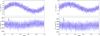 |
Fig. 5 Best fit for Si III λ4567 (left) and λ4574 (right) lines from mode identification with the MM for the SC1 RADIAL scenario with i = 60°, υe sin i = 100 km s−1, f = 5.25 d−1, and υamp = 21 km s−1 as inputs. The data are phase-folded according to the detected frequency. The observational data along with their error bars are shown in blue and the fit in red for the first (top) and second (bottom) moments of the time series. |
Best-fit parameters from single mode identifications.
5.2 Multimode configurations
SC3 MULTI-EQ. The frequency analysis requests an additional iteration to extract both frequencies. Both input frequencies are retrieved by each method. Despite equal-amplitude inputs, frequencies are retrieved with different Fourier amplitudes and detection order. The MM finds f1 prior to f2, while the FPF does the opposite. Subsequent mode identifications succeed by now fitting both modes, using the same parameter ranges as in scenario SC1 RADIAL, simultaneously. Parameters are consistent across lines and methods, however with an overestimation of inclination with the MM. The resulting fits for the Si III λ4567 line are displayed in Figs. 8a and b for the FPF method only. The corresponding parameters are provided in Table 5 for both methods and for both lines. Results for the Si III λ4574 line are given in Figs. B.4a and b.
The detection order between methods differs due to their differential sensitivity. The MM favours global changes while the FPF favours local ones. These results highlight the feasibility of unambiguous multimode identification. However, we note that fixing inclination to its input sometimes creates issues (in this case for the λ4567 line only) with the geometric parameters and overestimates velocity amplitudes.
SC4 MULTI-LOW. Despite the intrinsic amplitude disparity between the modes, the frequency analysis outcome for the Si III λ4567 line is similar to the previous case. This in contrast alters the significance of f2 for the λ4574 line with the FPF method. Still, we included it in mode identification to investigate potential impact that frequencies under the significance level could have on the process. We set υamp2 to the range [1:10] km s−1 with a step of 1 km s−1. All the multimode identifications were successful, despite the amplitude disparity and the inclusion of a frequency below the adopted significance threshold. The results from this configuration with the FPF method are displayed in Figs. 8a–c while the best-fitting parameters for both methods and both lines are given in the second half of Table 5. Results associated with Si III λ4574 line are given in Figs. B.4a–c.
A weaker amplitude complicates the mode identification due to an increased impact from the noise. This is indeed the case and visible in the observed amplitude and phase profiles of the sectoral modes in Figs. 8c and B.44c. Despite this, both frequencies are still identified for the λ4567 line while f2 is deemed as insignificant by the FPF for the λ4574 line. This likely results from the combination of noise affecting local variations and the line being weaker than the previous one. Our current threshold criteria rely on ground-based observations and may not suit space-based campaigns, for which lower thresholds might be more appropriate due to better observing conditions (see the discussion in Bowman & Michielsen 2021). This, along with the complementarity of both methods and previous studies of the prioritised targets (Bowman et al. 2022), justifies our choice to include f2 in mode identification. Its inclusion did not hinder mode identification, despite it being noisier and its lack of significance. Fixing inclination troubles the λ4567 modes geometry in some models, while the MM method can resolve or, in some cases, disturb other parameters.
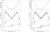 |
Fig. 6 Best fit for Si III λ4567 (left) and λ4574 (right) lines resulting from mode identification with the FPF method for a single radial mode configuration with i = 60°, υe sin i = 100 km s−1, f = 5.25 d−1, and υamp = 21 km s−1 as inputs. The FPF method fits a model (red line) to the observational (blue line) zero-point (top panel), amplitude (middle panel) and phase (bottom panel) profiles for each detected pulsation frequency mode. The statistical uncertainty range of the observations and the model are shown by the green and red shaded areas, respectively. |
5.3 Rotation
SC5 SLOW-ROT. Within a lower rotational regime of 10 km s−1, we lack a broadened spectral line from rotation. Broader lines benefit from the FPF method, which is confirmed by attempting to fit the lines. In addition to both input frequencies, spurious significant peaks are detected. Despite only including known input frequencies in the mode identification, we could not fit the zero-point profile of the lines. We thus fully relied on the MM, with which we succeeded in fitting both modes simultaneously and retrieved geometric parameters. The best-fit models correctly constrain inclination to its input value, slightly underestimate υe sin i, while slightly overestimating both velocity amplitudes.
Multimode identifications revealed to be successful in each case. Confronting results from the different multimode scenarios in terms of amplitude disparity reveals that a low amplitude mode is the culprit factor in challenging frequency retrieval and mode identification rather than having multiple interacting modes per se. Also, the inclusion of an input frequency below the adopted significant threshold did not impact mode identification. Within the mode identification process, we had to remain particularly careful about the inclination parameter. It plays an important role in the degeneracy of the computed solutions, and fixing it to its input can sometimes improve the geometric parameters while sometimes introduce disagreements among models, or cause best-fitting models to converge towards incorrect spherical harmonic geometries. For sufficiently fast-rotating stars, we summarise that the FPF method is more robust than the MM.
5.4 Intrinsic amplitude and significance threshold
SC6 AMP-THRESH. We find that a low amplitude is the main factor challenging mode identification. To support this conclusion, we investigated the impact of the intrinsic velocity amplitude of a mode on its frequency detectability and significance in. We monitored the S/N of the input frequency f1(S/Nf), computed as the amplitude of the Fourier peak divided by the mean noise of the pre-whitened signal around f1. The results from radial, sectoral and tesseral modes are gathered in Fig. 9, where each spherical harmonic geometry is investigated with both methods and for both Si III lines. The relative strength between the lines is reflected in the data with higher S /Nf values for the λ4567 line, which is the strongest and displays stronger effects from pulsations. In addition, the difference between methods is due to the global or local nature of the quantities being monitored, which explains the lower scale for the FPF method.
For the radial mode (top panels of Fig. 9), the peak S/Nf increases linearly with the intrinsic velocity amplitude of the mode. The key difference between the methods appears at low amplitudes: the FPF results fall below the significance threshold and lack structure, indicating a noise-dominated regime. In contrast, the MM remains sensitive to global changes in the line profile caused by the radial mode, allowing it to retain significance. The sectoral mode (middle panels of Fig. 9) shows a similar trend among methods. At low amplitudes, the FPF method is again noise-dominated and under the significance threshold but unlike the radial mode, the trend remains linear. It shows that the FPF method is more sensitive to local features in the line profile caused by higher-(l, m) geometries. We find a drastic difference between the methods for the tesseral mode (bottom panels of Fig. 9). The MM completely fails at detecting the input frequency peak in Fourier spectra as they are completely noise dominated. In contrast, the FPF method not only succeeds in detecting the peak, but does so above the significance threshold even at low intrinsic velocities. Due to the complex geometry of the mode, the features affecting the line profile are now too subtle to be detected by the moments, making now the FPF the only alternative to measure the frequencies and identify such mode geometries.
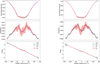 |
Fig. 7 Best fit for Si III λ4567 (left) and λ4574 (right) lines resulting from mode identification with the FPF method for a single tesserai (l, m) = (8,6) mode configuration with i = 60°, υe sin i = 100 km s−1, f = 5.25 d−1, and υamp = 21 km s−1 as inputs. The FPF method fits a model (red line) to the observational (blue line) zero-point (top panel), amplitude (middle panel), and phase (bottom panel) profiles for each detected pulsation frequency mode. The statistical uncertainty range of the observations and the model are shown by the green and red shaded areas, respectively. |
5.5 Orbital sampling scenarios
The results of the frequency analysis are gathered in Table 6 and organised per sampling scenario, previously described in Sect. 4.
5.5.1 Cadence and sampling
SC7 RAND-VIS. By introducing randomness in the single observation taken every orbit, both frequencies are detected. However, the FPF method detects f2 below the adopted significant threshold.
In addition to the low amplitude and the stronger noise contribution compared to the MM, the FPF now also faces irregularities in the sampling of the data. Such irregularity leads to a more complex spectral window, producing many alias components that redistribute power away from the central peak (Eyer & Bartholdi 1999). This reduces the prominence of the real frequency and effectively increases the background noise level, making mode identification more difficult. The relative impact of the noise is therefore even stronger, disadvantaging the significance of f2 compared to the case of the regular sampling (SC4).
We note, however, that irregular sampling has its advantages. Unlike strictly regular sampling, it avoids a strict Nyquist limit, making the maximum detectable frequency limited by exposure times rather than cadence. For β Cephei pulsators this distinction is, however, not critical, since their frequencies are typically below the expected Nyquist limit for CubeSpec’s cadence (see Burssens et al. 2020; Bowman et al. 2022 for catalogues).
SC8 BOOST-CAD. This scenario results in approximately having two observations per orbit, still randomly selected within target’s visibility. The increased sampling resolves the earlier significance issue of f2, which is now restored. To disentangle the impact of a higher cadence from the number of observations on the significance restoration, we repeated this test over a time span of 45 d, keeping the number of data points similar to SC7. In this setup, f2 also regains significance, albeit only marginally, confirming that the higher cadence is the dominant factor over the total number of observations.
From this baseline, we investigated which factor - the sampling of pulsations or the data quality - has a larger impact on the significant detection of frequencies. The improvement from the former already highlights the importance of a denser sampling of pulsation cycles for significant retrieval of frequencies. In summary, randomness in the data impacts the significance of the frequency while a denser sampling improves it.
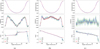 |
Fig. 8 Best fit for Si III λ4567 line mode identifications performed with the FPF method in multimode configuration with i = 60°, υe sin i = 100 km s−1, fi = 5.25 d−1, (l1, m1) = (0,0), υampl = 21 km s−1, f2 = 5.385 d−1, (l2, m2) = (2,2), and υamp2 = 21 or 3 km s−1 as inputs. The multimode model fits the zero-point (top), amplitude (middle), and phase (bottom) profiles for the radial (a), 21 km s−1 sectoral (b), and 3 km s−1 sectoral (c) modes. |
Best-fit parameters from multimode identifications.
5.5.2 Data quality
SC9 ADAPT-S/N. The observational series produces a mix of higher- and lower-S/N spectra. The latter contribute to the time series approximately twice as much as the former. Again, this increase in observations restores f2 significance lost in the baseline scenario SC7, involving a single random observation per orbit.
In addition to the results of the previous test (SC8), having more (albeit lower-quality) spectra in the observations supports the previous argument. That is, a greater importance from the sampling cadence than uniform high-quality exposures over the significant detection of frequencies. From these scenarios, we can conclude that an efficient sampling of the pulsations’ phases has more of an impact on successful significant frequency retrieval and must be prioritised over data quality in the scheduling of the mission.
SC10 SHORT-FULL. Again with a single observation randomly made per orbit, the time span of the mission is reduced to 30 d. Despite the sharp fall in the number of observations, the outcome is similar to the 90 d mission: f2 is under the significance level according to the FPF method.
SC11 SHORT-HALF. Degrading both the time span and the quality of the data breaks the objective of the mission. Under these conditions, neither the MM or FPF method successfully retrieves f2, and spurious peaks appear in the frequency spectra.
By first decreasing the duration of the mission, we were able to determine the relative importance of the total time span of the mission compared to the cadence of the sampling. Again, we find that the latter is the more important for frequency retrieval; the result is similar to that for the 90 d time span. Finally, we also establish that a short time span combined with degraded data defines a lower operational threshold where frequency retrieval becomes unreliable. Especially, this also sets a limit estimation on the requested data quality to recover frequencies, particularly for low intrinsic velocity amplitudes.
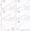 |
Fig. 9 Frequency peak S/Nf against its input intrinsic velocity amplitude for radial (top panels), sectoral (l, m) = (2,2) (middle panels), and tesserai (l, m) = (8,6) (bottom panels) modes. Both Si III λ4567 (blue) and λ4574 (red) lines are investigated with the MM (left) and FPF (right) methods. Symbols represent the measured data and the dashed lines the resulting fits. The horizontal dashed black line shows the frequency peak significance threshold used throughout the study. |
5.6 Impact of the Moon
All previous scenarios are repeated to account for a more realistic campaign by including lunar interruptions. As explained in Sect. 2.4, a Moon avoidance angle of 20° (see Fig. 4) is imposed to avoid excessive stray light. It results in forbidden visibility windows, or gaps, for some of the targets (e.g. this is the case for τ Lib while β Cep is not impacted). From the visibility schedule of τ Lib, the Moon causes interruptions of approximately 3 d every 30 d. It induces a data loss of approximately 10% of the initial dataset. The results of the analyses including lunar interruptions are also provided in Table 6. For the scenarios we tested, the inclusion of the Moon does not alter the analysis results.
Given the lack of impact caused by the Moon interruptions, this should not be an obstacle with regard to frequency retrieval and significant detection. We mention nevertheless that it slightly contributes to the average noise level in the Fourier data and therefore increases the significance criterion level.
By the time CubeSpec spectroscopy becomes available, most bright β Cephei targets will already have well-established frequency spectra from space-based (e.g. BRITE and TESS; Weiss et al. 2014) and/or ground-based photometry, and gathered in Bowman et al. 2022. This reduces the emphasis on peak significance, as even lower-amplitude detections can be identified as real from already known frequencies. Moreover, CubeSpec time series spectroscopy offers access to higher-degree modes that are nearly invisible in photometry, especially in stars with low inclination where geometric cancellation suppresses sectoral modes.
Results of the frequency analysis for the described observational scenarios.
6 Conclusions
In this work, we investigated the asteroseismic observational strategy for the upcoming CubeSpec space mission (Raskin et al. 2018; Bowman et al. 2022) through a series of simulations that replicate expected spectroscopic time series. Our LPV simulator, based on TLUSTY model atmospheres and FAMIAS pulsation profiles, realistically models β Cephei variability, incorporating both stellar and instrumental effects, including noise, cadence, and observational constraints.
From simulated time series, we demonstrate that the expected data quality of S/N ≈ 140 per pixel obtained with texp = 15 min for Vmag = 4 targets is sufficient to retrieve pulsation frequencies and identify pulsation mode spherical harmonic geometries, even in complex and/or multimode scenarios, using the Si III lines. Both the MM and the FPF method succeed in identifying radial and non-radial modes; the FPF method is particularly robust for higher-degree geometries and multimode configurations, even at low amplitudes. The MM, on the other hand, remains a reliable fallback for slow rotators, for which FPF becomes ineffective, i.e. when pulsational broadening dominates over rotational broadening (Aerts & De Cat 2003; Bowman et al. 2022). With proper parameter refinement, successful mode identification remains feasible. We stress the importance of carefully handling the inclination parameter in the identification process, as it heavily influences the degeneracy and stability of the derived solutions.
Irregular sampling cadence, resulting from realistic orbital visibility, can impact the detection significance of loweramplitude modes. However, such an issue can be mitigated by increasing the sampling rate, though potentially at the detriment of the S/N quality of additional spectra in the time series. Also, lunar obstructions are not considered as an obstacle for the observational campaign.
Our simulations allowed us to translate detection thresholds into guidelines for CubeSpec’s strategy, accounting for the fact that ensuring the overall goals of the mission on at least a few targets prevails over the observed targets quantity. To guarantee both frequency and unambiguous multimode identifications, we therefore recommend using the SC8 scenario. The SC8 strategy ensures the significant detection of multimode and/or higher-order frequencies and is the most robust of the tested scenarios. The number of targets feasible in such conditions within an orbit is estimated to be between 3 and 5, depending on the needed exposure time. This is sufficient to explore different physics regimes, such as by targeting a fast rotator, a slow rotator, and a β Cephei in a binary system.
However, we also demonstrate that, with SC10, a single month of data might be enough to guarantee the detectability of the frequencies in favourable conditions. The recommended strategy therefore leads to a hybrid plan of action: we suggest starting with SC8 for a month to leverage the higher cadence for frequency detection and mode identification. Depending on the outcome, one can then continue with the SC8 strategy, move to a single exposure per orbit (SC7), or move to new targets following the SC10 strategy. Given that some physical effects have not been included (e.g. high rotation and binarity), our simulations remain idealised. Real-time evaluation of the in-flight data quality might therefore affect these conclusions. Furthermore, additional instrumental effects might only become apparent once the mission is in flight, at which point the CubeSpec team will need to re-evaluate the final sampling strategy.
Acknowledgements
CubeSpec is an ESA GSTP mission, funded by the Belgian Science Policy BELSPO. The research leading to these results has received funding from the European Research Council (ERC) under the European Union’s Horizon 2020 and Horizon Europe research and innovation programme (grant agreement numbers 772225: MULTIPLES). This research is also supported by the Flemish Government under the long-term structural Methusalem funding program, project SOUL: Stellar evolution in full glory, grant METH/24/012 at KU Leuven. It is also supported by from the Research Foundation - Flanders (FWO) (grant agreement G0ABL24N) and from the KU Leuven Research Council through grant iBOF/21/084. DMB acknowledges UK Research and Innovation (UKRI) in the form of a Frontier Research grant under the UK government’s ERC Horizon Europe funding guarantee (SYMPHONY; PI: Bowman; grant number: EP/Y031059/1), and a Royal Society University Research Fellowship (PI: Bowman; grant number: URF\R1\231631).
References
- Abbott, B. P., Abbott, R., Abbott, T. D., et al. 2016, ApJ, 818, L22 [Google Scholar]
- Aerts, C., & De Cat, P. 2003, Space Sci. Rev., 105, 453 [CrossRef] [Google Scholar]
- Aerts, C., Mathias, P., Gillet, D., & Waelkens, C. 1994, A&A, 286, 109 [NASA ADS] [Google Scholar]
- Aerts, C., Van Hoolst, T., & Mathias, P. 1995, in International Astronomical Union Colloquium, 155 (Cambridge University Press), 56 [Google Scholar]
- Aerts, C., Lehmann, H., Briquet, M., et al. 2003, A&A, 399, 639 [NASA ADS] [CrossRef] [EDP Sciences] [Google Scholar]
- Aerts, C., Christensen-Dalsgaard, J., & Kurtz, D. W. 2010, Asteroseismology (New York: Springer-Verlag) [Google Scholar]
- Auvergne, M., Bodin, P., Boisnard, L., et al. 2009, A&A, 506, 411 [NASA ADS] [CrossRef] [EDP Sciences] [Google Scholar]
- Balona, L. A., Aerts, C., & Stefl, S. 1999, MNRAS, 305, 519 [NASA ADS] [CrossRef] [Google Scholar]
- Blomme, R., Mahy, L., Catala, C., et al. 2011, A&A, 533, A4 [NASA ADS] [CrossRef] [EDP Sciences] [Google Scholar]
- Borucki, W., Koch, D., Basri, G., et al. 2010, Science, 327, 977 [CrossRef] [PubMed] [Google Scholar]
- Bowman, D. M. 2020, Front. Astron. Space Sci., 7, 70 [Google Scholar]
- Bowman, D. M. 2023, Ap&SS, 368, 107 [NASA ADS] [CrossRef] [Google Scholar]
- Bowman, D. M., & Michielsen, M. 2021, A&A, 656, A158 [NASA ADS] [CrossRef] [EDP Sciences] [Google Scholar]
- Bowman, D. M., Aerts, C., Johnston, C., et al. 2019a, A&A, 621, A135 [NASA ADS] [CrossRef] [EDP Sciences] [Google Scholar]
- Bowman, D. M., Burssens, S., Pedersen, M. G., et al. 2019b, Nat. Astron., 3, 760 [Google Scholar]
- Bowman, D. M., Vandenbussche, B., Sana, H., et al. 2022, A&A, 658, A96 [NASA ADS] [CrossRef] [EDP Sciences] [Google Scholar]
- Bradt, H. 2003, Astronomy Methods: A Physical Approach to Astronomical Observations (Cambridge University Press) [Google Scholar]
- Briquet, M., & Aerts, C. 2003, A&A, 398, 687 [NASA ADS] [CrossRef] [EDP Sciences] [Google Scholar]
- Burssens, S., Simón-Díaz, S., Bowman, D. M., et al. 2020, A&A, 639, A81 [NASA ADS] [CrossRef] [EDP Sciences] [Google Scholar]
- Burssens, S., Bowman, D. M., Michielsen, M., et al. 2023, Nat. Astron., 7, 913 [NASA ADS] [CrossRef] [Google Scholar]
- Catanzaro, G., & Leone, F. 2008, MNRAS, 389, 1414 [NASA ADS] [CrossRef] [Google Scholar]
- Degroote, P., Aerts, C., Ollivier, M., et al. 2009, A&A, 506, 471 [NASA ADS] [CrossRef] [EDP Sciences] [Google Scholar]
- Eyer, L., & Bartholdi, P. 1999, A&AS, 135, 1 [NASA ADS] [CrossRef] [EDP Sciences] [Google Scholar]
- Hubeny, I. 1988, Comput. Phys. Commun., 52, 103 [Google Scholar]
- Hubeny, I., & Lanz, T. 2017, arXiv e-prints [arXiv:1706.01859] [Google Scholar]
- Langer, N. 2012, ARA&A, 50, 107 [CrossRef] [Google Scholar]
- Lanz, T., & Hubeny, I. 2007, ApJS, 169, 83 [CrossRef] [Google Scholar]
- Mazumdar, A., Briquet, M., Desmet, M., & Aerts, C. 2006, A&A, 459, 589 [NASA ADS] [CrossRef] [EDP Sciences] [Google Scholar]
- Raskin, G., Delabie, T., De Munter, W., et al. 2018, SPIE, 10698, 106985R [Google Scholar]
- Ricker, G. R., Winn, J. N., Vanderspek, R., et al. 2015, J. Astron. Telesc. Instrum. Syst., 1, 014003 [Google Scholar]
- Schroeder, D. J. 2000, in Astronomical Optics, 2nd edn., ed. D. J. Schroeder (San Diego: Academic Press), 321 [Google Scholar]
- Stürmer, J., Seifahrt, A., Robertson, Z., Schwab, C., & Bean, J. L. 2019, PASP, 131, 024502 [Google Scholar]
- Vandenbussche, B., Sana, H., Raskin, G., et al. 2021, in 43rd COSPAR Scientific Assembly, Held 28 January-4 February, 43, 1509 [Google Scholar]
- Weiss, W. W., Rucinski, S. M., Moffat, A. F. J., et al. 2014, PASP, 126, 573 [Google Scholar]
- Wofford, A., Leitherer, C., Walborn, N. R., et al. 2012, arXiv e-prints [arXiv:1209.3199] [Google Scholar]
- Zima, W. 2006, A&A, 455, 227 [NASA ADS] [CrossRef] [EDP Sciences] [Google Scholar]
- Zima, W. 2008, Commun. Asteroseismol., 155, 17 [Google Scholar]
Appendix A Spectral format
Spectral order numbers and the starting, central, and ending wavelengths.
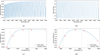 |
Fig. A.1 (a): Optical transmission, T(λ), obtained from Eq. 1. (b): Blaze function of the grating computed according to Eq. 2. (c): Mirror reflectivity for the (U, B, V, R, and I) bands (red dots) and complete quadratic interpolation (blue line). The CubeSpec range limits are indicated by the two dashed grey lines. (d): Quantum efficiency for the (U, B, V, R, and I) bands (red dots) and complete quadratic interpolation (blue line). The CubeSpec range limits are indicated by the two dashed grey lines. |
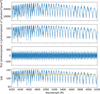 |
Fig. A.2 Noise and S/N distributions obtained with Vmag = 4 and texp = 15 min. Top panel: Variance (σ2) of the 1D simulated flux obtained by summing the different noise contributions in quadrature according to Eq. 7. Second panel: Standard deviation (σ) of the 1D simulated flux. Third panel: Noise spectrum obtained by setting its standard deviation as computed in the previous panel. Fourth panel: Synthetic S/N spectrum over the complete spectral range of CubeSPEC, obtained by dividing the 1D signal by its standard deviation. The horizontal orange line shows the median S/N. |
Appendix B Additional results
Appendix B.1 Si III λ4553 and He I λ5876 lines
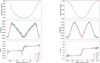 |
Fig. B.1 Best fit for Si III λ4553 (left) and He I λ5876 (right) lines resulting from mode identification with the FPF method for a single radial mode configuration with i = 60°, υe sin i = 100 km s−1, f = 5.25 d−1, and υamp = 21 kms−1 as inputs. The FPF method fits a model (red line) to the observational (blue line) zero-point (top panel), amplitude (middle panel), and phase (bottom panel) profiles for each detected pulsation frequency mode. The statistical uncertainty range of the observations and the model are shown by the red and green shaded areas, respectively. |
Best-fit parameters from radial mode identifications for Si III λ4553 and He I λ5876 lines.
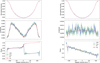 |
Fig. B.2 Best fit for Si III λ4553 line mode identifications performed with the FPF method in multimode configuration with i = 60°, υe sin i = 100 km s−1, f1 = 5.25 d−1, (11, m1) = (0,0), υamp1 = 21 km s−1, f2 = 5.385 d−1, (l2, m2) = (2,2), and υamp2 = 21kms−1 as inputs. The multimode model fits the zero-point (top panels), amplitude (middle panels), and phase (bottom panels) profiles for the radial (left) and sectoral (right) modes. |
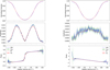 |
Fig. B.3 Best fit for He I λ5876 line mode identifications performed with the FPF method in multimode configuration with i = 60°, υe sin i = 100 km s−1, f1 = 5.25 d−1, (11, m1) = (0,0), υamp1 = 21 km s−1, f2 = 5.385 d−1, (12,m2) = (2,2), and υamp2 = 21kms−1 as inputs. The multimode model fits the zero-point (top panels), amplitude (middle panels), and phase (bottom panels) profiles for the radial (left) and sectoral (right) modes. |
Optimised parameters of the best fit resulting from multimode identification performed with the FPF method for each spectral line.
Appendix B.2 Si III λ4574 line multimode results
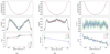 |
Fig. B.4 Best fit for Si III λ4574 line mode identifications performed with the FPF method in multimode configuration with i = 60°, υe sin i = 100 km s−1, f1 = 5.25 d−1, (11, m1) = (0,0), υamp1 = 21 km s−1, f2 = 5.385 d−1, (12,m2) = (2,2), and υamp2 = 21 or 3km s−1 as inputs. The multimode model fits the zero-point (top panels), amplitude (middle panels), and phase (bottom panels) profiles for the radial (a), 21 km s−1 sectoral (b), and 3 km s−1 sectoral (c) modes. |
All Tables
Numerical values of the instrumental parameters discussed in the main text, used for scaling the TLUSTY spectrum before convolution, noise, and stray light computation.
Pulsation-independent parameter ranges [start:end] or values, obtained after iterating, to fit the zero-point profile with the FPF method before mode identification.
Best-fit parameters from radial mode identifications for Si III λ4553 and He I λ5876 lines.
Optimised parameters of the best fit resulting from multimode identification performed with the FPF method for each spectral line.
All Figures
|
Fig. 1 (a) TLUSTY model atmosphere with Teff = 27 000 K, log g = 4.0, Vt = 2 km s−1, and Z = Z⊙ over the CubeSpec spectral range scaled to Vmag = 4. We show the astrophysical flux (blue) and corresponding continuum (orange). (b) Effective flux from Eq. (5) (blue) and corresponding continuum (orange). (c) Detector counts per pixel from Eq. (6) (blue) and corresponding continuum (orange). (d) Normalised spectrum. |
| In the text | |
|
Fig. 2 Left: noise budget contributors: total (blue), shot (orange), stray light (green), readout (red), dark current (purple), and pixel gain variability (brown). Right: portion of the simulated, not convolved, spectrum after the addition of the noise. The focus is on spectral order 84, which contains the Si III triplet around λ4553, λ4567, and λ4574 lines and is used for asteroseismic diagnosis. |
| In the text | |
|
Fig. 3 Si III λ4574 line time series assuming an inclination of 60°, a projected rotational velocity (υe sin i) of 100 km s−1, a cadence of 90 min, and an exposure time (texp) of 15 min at Vmag = 4, resulting in a S/N of ≈ 140. Left panel: multimode configuration: a radial mode at 5.25 d−1 with an intrinsic velocity amplitude (υamp1) of 21 km s−1 and a sectoral l = m = 2 mode at 5.385 d−1 with υamp2 = 21 km s−1. Right panel: single mode configuration: a tesseral (l, m) = (8,6) mode at 5.25 d−1 and with υamp = 21 km s−1. The dashed red lines show the noiseless profiles, and the blue lines show the average profile of each series. |
| In the text | |
|
Fig. 4 Left: avoidance angles for CubeSpec. The grey shaded spacecraft is displayed at three positions along its orbit, assuming the optical axis is pointing in the anti-Sun direction. The green shades illustrate the regions of the sky accessible from each of those locations. The Moon is seen partly obstructing one of those regions. The zones of avoidance imposed by the Sun, the Earth, and CubeSpec’s radiator are shown in yellow, blue, and red, respectively. Right: simulated evolution of visibility window duration over 6 months of visibility of the star τ Lib, involving lunar interruptions. The vertical lines show the start (blue) of the observational campaign and the ends of 90 d (red) and 30 d (black) observational campaigns defined for the observing scenarios described in the main text (Sect. 3). The inset panel zooms into the start of visibility to highlight visibility windows. |
| In the text | |
|
Fig. 5 Best fit for Si III λ4567 (left) and λ4574 (right) lines from mode identification with the MM for the SC1 RADIAL scenario with i = 60°, υe sin i = 100 km s−1, f = 5.25 d−1, and υamp = 21 km s−1 as inputs. The data are phase-folded according to the detected frequency. The observational data along with their error bars are shown in blue and the fit in red for the first (top) and second (bottom) moments of the time series. |
| In the text | |
|
Fig. 6 Best fit for Si III λ4567 (left) and λ4574 (right) lines resulting from mode identification with the FPF method for a single radial mode configuration with i = 60°, υe sin i = 100 km s−1, f = 5.25 d−1, and υamp = 21 km s−1 as inputs. The FPF method fits a model (red line) to the observational (blue line) zero-point (top panel), amplitude (middle panel) and phase (bottom panel) profiles for each detected pulsation frequency mode. The statistical uncertainty range of the observations and the model are shown by the green and red shaded areas, respectively. |
| In the text | |
|
Fig. 7 Best fit for Si III λ4567 (left) and λ4574 (right) lines resulting from mode identification with the FPF method for a single tesserai (l, m) = (8,6) mode configuration with i = 60°, υe sin i = 100 km s−1, f = 5.25 d−1, and υamp = 21 km s−1 as inputs. The FPF method fits a model (red line) to the observational (blue line) zero-point (top panel), amplitude (middle panel), and phase (bottom panel) profiles for each detected pulsation frequency mode. The statistical uncertainty range of the observations and the model are shown by the green and red shaded areas, respectively. |
| In the text | |
|
Fig. 8 Best fit for Si III λ4567 line mode identifications performed with the FPF method in multimode configuration with i = 60°, υe sin i = 100 km s−1, fi = 5.25 d−1, (l1, m1) = (0,0), υampl = 21 km s−1, f2 = 5.385 d−1, (l2, m2) = (2,2), and υamp2 = 21 or 3 km s−1 as inputs. The multimode model fits the zero-point (top), amplitude (middle), and phase (bottom) profiles for the radial (a), 21 km s−1 sectoral (b), and 3 km s−1 sectoral (c) modes. |
| In the text | |
|
Fig. 9 Frequency peak S/Nf against its input intrinsic velocity amplitude for radial (top panels), sectoral (l, m) = (2,2) (middle panels), and tesserai (l, m) = (8,6) (bottom panels) modes. Both Si III λ4567 (blue) and λ4574 (red) lines are investigated with the MM (left) and FPF (right) methods. Symbols represent the measured data and the dashed lines the resulting fits. The horizontal dashed black line shows the frequency peak significance threshold used throughout the study. |
| In the text | |
|
Fig. A.1 (a): Optical transmission, T(λ), obtained from Eq. 1. (b): Blaze function of the grating computed according to Eq. 2. (c): Mirror reflectivity for the (U, B, V, R, and I) bands (red dots) and complete quadratic interpolation (blue line). The CubeSpec range limits are indicated by the two dashed grey lines. (d): Quantum efficiency for the (U, B, V, R, and I) bands (red dots) and complete quadratic interpolation (blue line). The CubeSpec range limits are indicated by the two dashed grey lines. |
| In the text | |
|
Fig. A.2 Noise and S/N distributions obtained with Vmag = 4 and texp = 15 min. Top panel: Variance (σ2) of the 1D simulated flux obtained by summing the different noise contributions in quadrature according to Eq. 7. Second panel: Standard deviation (σ) of the 1D simulated flux. Third panel: Noise spectrum obtained by setting its standard deviation as computed in the previous panel. Fourth panel: Synthetic S/N spectrum over the complete spectral range of CubeSPEC, obtained by dividing the 1D signal by its standard deviation. The horizontal orange line shows the median S/N. |
| In the text | |
|
Fig. B.1 Best fit for Si III λ4553 (left) and He I λ5876 (right) lines resulting from mode identification with the FPF method for a single radial mode configuration with i = 60°, υe sin i = 100 km s−1, f = 5.25 d−1, and υamp = 21 kms−1 as inputs. The FPF method fits a model (red line) to the observational (blue line) zero-point (top panel), amplitude (middle panel), and phase (bottom panel) profiles for each detected pulsation frequency mode. The statistical uncertainty range of the observations and the model are shown by the red and green shaded areas, respectively. |
| In the text | |
|
Fig. B.2 Best fit for Si III λ4553 line mode identifications performed with the FPF method in multimode configuration with i = 60°, υe sin i = 100 km s−1, f1 = 5.25 d−1, (11, m1) = (0,0), υamp1 = 21 km s−1, f2 = 5.385 d−1, (l2, m2) = (2,2), and υamp2 = 21kms−1 as inputs. The multimode model fits the zero-point (top panels), amplitude (middle panels), and phase (bottom panels) profiles for the radial (left) and sectoral (right) modes. |
| In the text | |
|
Fig. B.3 Best fit for He I λ5876 line mode identifications performed with the FPF method in multimode configuration with i = 60°, υe sin i = 100 km s−1, f1 = 5.25 d−1, (11, m1) = (0,0), υamp1 = 21 km s−1, f2 = 5.385 d−1, (12,m2) = (2,2), and υamp2 = 21kms−1 as inputs. The multimode model fits the zero-point (top panels), amplitude (middle panels), and phase (bottom panels) profiles for the radial (left) and sectoral (right) modes. |
| In the text | |
|
Fig. B.4 Best fit for Si III λ4574 line mode identifications performed with the FPF method in multimode configuration with i = 60°, υe sin i = 100 km s−1, f1 = 5.25 d−1, (11, m1) = (0,0), υamp1 = 21 km s−1, f2 = 5.385 d−1, (12,m2) = (2,2), and υamp2 = 21 or 3km s−1 as inputs. The multimode model fits the zero-point (top panels), amplitude (middle panels), and phase (bottom panels) profiles for the radial (a), 21 km s−1 sectoral (b), and 3 km s−1 sectoral (c) modes. |
| In the text | |
Current usage metrics show cumulative count of Article Views (full-text article views including HTML views, PDF and ePub downloads, according to the available data) and Abstracts Views on Vision4Press platform.
Data correspond to usage on the plateform after 2015. The current usage metrics is available 48-96 hours after online publication and is updated daily on week days.
Initial download of the metrics may take a while.