| Issue |
A&A
Volume 705, January 2026
|
|
|---|---|---|
| Article Number | A76 | |
| Number of page(s) | 17 | |
| Section | Extragalactic astronomy | |
| DOI | https://doi.org/10.1051/0004-6361/202556376 | |
| Published online | 07 January 2026 | |
ZTF SN Ia DR2 follow-up: Exploring the origin of the Type Ia supernova host galaxy step through Si II velocities
1
School of Physics, Trinity College Dublin, College Green, Dublin 2, Ireland
2
Institute of Space Sciences (ICE-CSIC), Campus UAB, Carrer de Can Magrans, s/n, E-08193 Barcelona, Spain
3
Institut d’Estudis Espacials de Catalunya (IEEC), 08860 Castelldefels (Barcelona), Spain
4
Université Lyon, CNRS, IP2I Lyon/IN2P3, UMR 5822, F-69622 Villeurbanne, France
5
Department of Astronomy & Center for Galaxy Evolution Research, Yonsei University, Seoul, 03722
Republic of Korea
6
Oskar Klein Centre, Department of Astronomy, Stockholm University, SE-10691 Stockholm, Sweden
7
Instituto de Ciencias Exactas y Naturales (ICEN), Universidad Arturo Prat, Iquique, Chile
8
Department of Physics, Lancaster University, Lancaster, LA1 4YB
UK
9
The Oskar Klein Centre, Department of Physics, Stockholm University, SE-10691 Stockholm, Sweden
10
Institut für Physik, Humboldt-Universität zu Berlin, Newtonstr. 15, 12489 Berlin, Germany
11
Lawrence Berkeley National Laboratory, 1 Cyclotron Road MS 50B-4206, Berkeley, CA, 94720
USA
12
Department of Astronomy, University of California, Berkeley, 501 Campbell Hall, Berkeley, CA, 94720
USA
13
Caltech Optical Observatories, California Institute of Technology, Pasadena, CA, 91125
USA
14
Division of Physics, Mathematics and Astronomy, California Institute of Technology, Pasadena, CA, 91125
USA
15
IPAC, California Institute of Technology, 1200 E. California Blvd, Pasadena, CA, 91125
USA
16
Department of Physics and Astronomy, Northwestern University, 2145 Sheridan Road, Evanston, IL, 60208
USA
17
Center for Interdisciplinary Exploration and Research in Astrophysics (CIERA), 1800 Sherman Ave., Evanston, IL, 60201
USA
18
NSF-Simons AI Institute for the Sky (SkAI), 172 E. Chestnut St., Chicago, IL, 60611
USA
★ Corresponding author: This email address is being protected from spambots. You need JavaScript enabled to view it.
Received:
11
July
2025
Accepted:
26
October
2025
Abstract
The relation between Type Ia supernovae (SNe Ia) and the stellar masses of their host galaxy is well documented. In particular, Hubble residuals display a distinct luminosity shift based on host mass. This is known as the mass step. This effect is widely used as an additional correction factor in the standardisation of SN Ia luminosities. We investigate the Hubble residuals and the mass step of normal SNe Ia in the context of Si IIλ6355 velocities based on 277 normal SNe Ia that are near their peak in the second data release (DR2) of the Zwicky Transient Facility (ZTF). We divided the sample into high-velocity (HV) and normal-velocity (NV) SNe Ia, separated at 12,000 km s−1. This produced a sample of 70 HV and 207 NV objects. We then explored potential environment- and/or progenitor-related effects by investigating the Si IIλ6355 velocities with parameters such as the light-curve stretch x1, the colour c, and the host galaxy properties. Although we only find a marginal difference between the Hubble residuals of HV and NV SNe Ia, the NV mass step is 0.149 ± 0.024 mag (6.3σ). The HV mass step is smaller, 0.046 ± 0.041 mag (1.1σ), and is consistent with zero. The difference between the NV and HV mass steps is modest, at ∼2.2σ. Moreover, the clearest subtype difference appears for SNe in central regions (dDLR < 1), where NV SNe Ia show a large mass step, whereas HV SNe Ia are consistent with no step, yielding a difference of 3.1–3.6σ between NV and HV SNe Ia. We observe a host-colour step for both subtypes. NV SNe Ia show a step of 0.142 ± 0.024 mag (5.9σ), while HV SNe Ia show a step of 0.158 ± 0.042 mag (3.8σ), where the HV SNe Ia step appears to be larger, but the significance is lower because the sample size is smaller. Overall, the NV and HV colour steps are statistically consistent. HV SNe Ia also show modest (∼2.5–3σ) steps in certain subsets, such as those in outer regions (dDLR > 1), whereas NV SNe display stronger environmental trends. Our results indicate that NV SNe Ia appear to be more environmentally sensitive, particularly in central likely metal-rich and older regions, while HV SNe Ia show weaker and subset-dependent trends. This suggests that applying a universal mass-step correction might introduce biases, and that incorporating refined classifications and/or environment-dependent factors, such as the location within the host, might improve future cosmological analyses beyond the standard x1 and c cuts.
Key words: supernovae: general
© The Authors 2026
 Open Access article, published by EDP Sciences, under the terms of the Creative Commons Attribution License (https://creativecommons.org/licenses/by/4.0), which permits unrestricted use, distribution, and reproduction in any medium, provided the original work is properly cited.
This article is published in open access under the Subscribe to Open model. This email address is being protected from spambots. You need JavaScript enabled to view it. to support open access publication.
1. Introduction
Type Ia supernovae (SNe Ia) are proven to be reliable distance estimators and are used as standardisable candles to measure extragalactic distances (Phillips 1993; Hamuy et al. 1995; Riess et al. 1996). This property has made them crucial in cosmology and led to the discovery of the accelerating expansion of the Universe (Riess et al. 1998; Perlmutter et al. 1999) and the measurement of the Hubble constant H0 (Riess et al. 2009; Freedman et al. 2019; Riess et al. 2022; Galbany et al. 2023).
Supernovae Ia exhibit an observed scatter of about 0.4 mag in MB (Branch & Miller 1993). This dispersion can be significantly reduced to approximately 0.15 mag by applying empirical corrections based on the brighter-slower and brighter-bluer correlations, however (Phillips 1993; Riess et al. 1996; Tripp 1998). These corrections are based on light-curve properties, specifically, on the stretch x1 and the colour c, which are commonly determined using light-curve fitting methods such as the Spectral Adaptive Lightcurve Template 2 (SALT2; Guy et al. 2007, 2010), the Spectral Adaptive Lightcurve Template 2 (SALT3; Kenworthy et al. 2021; Taylor et al. 2023), the SuperNovae in object-oriented Python (Burns et al. 2011, 2014, SNooPy), and the Bayesian Supernova model (BayeSN; Mandel et al. 2022; Grayling et al. 2024). Despite the improved scatter, however, an unknown source of uncertainty still remains, even when observational errors or theoretical limitations are accounted for.
Supernovae Ia are widely accepted as the thermonuclear explosions of carbon–oxygen (C/O) white dwarfs (WDs) in binary systems (Hoyle & Fowler 1960; Nugent et al. 2011; Maoz et al. 2014). Their progenitors and underlying explosion mechanisms remain not fully understood, however (e.g. Maeda & Terada 2016; Jha et al. 2019; Ruiter & Seitenzahl 2025). Currently, there are two prevailing progenitor models for SNe Ia: the single-degenerate (SD) model (Whelan & Iben 1973; Nomoto et al. 1997), in which a C/O WD accretes material from a non-degenerate companion, such as a main-sequence star or an evolved red giant, and the double-degenerate (DD) model (Iben & Tutukov 1984; Webbink 1984), which involves the merger of two WDs. Multiple explosion mechanisms can also lead to a SN Ia in the DD model, such as the double-detonation scenario (Fink et al. 2007; Sim et al. 2010; Shen et al. 2018) and the violent merger scenario (Raskin et al. 2009; Pakmor et al. 2013; Sato et al. 2015; Roy et al. 2022).
SNe Ia are widely diverse in photometry and spectroscopy. This variation can affect their use in precision cosmology and makes it important to investigate different subtypes. In an effort to address this, Wang et al. (2009) introduced a classification system for normal cosmologically useful SNe Ia based solely on the velocity of the Si IIλ6355 absorption feature around peak brightness. In this scheme, SNe Ia with expansion velocities (vSi), above approximately 12,000 km s−1 are categorised as high-velocity (HV) SNe Ia, while those with lower velocities fall into the normal velocity (NV) group. This variation in velocity was also suggested to be independent of the evolution of the light curve, and it was suggested that the variation might result from differences in viewing angle (Maeda et al. 2010). Studies also suggested that HV SNe Ia exhibit distinct characteristics, including differences in light-curve evolution (Wang et al. 2008, 2009; Burgaz et al. 2021), a shorter time interval from explosion to peak brightness (Ganeshalingam et al. 2011), and intrinsically redder B–V colours (Pignata et al. 2008). Additionally, HV SNe Ia may follow different extinction laws (Wang et al. 2009; Foley & Kasen 2011). In contrast to previous studies that proposed that HV SNe Ia are mainly found in massive galaxies (Wang et al. 2013; Pan et al. 2015; Pan 2020; Dettman et al. 2021), Burgaz et al. (2025b) demonstrated in a volume-limited sample that HV SNe Ia do not necessarily favour high-mass galaxies, but are indeed also found in low-mass galaxies at a similar rate as NV SNe Ia. The authors further suggested that rather than representing a distinct population, HV SNe Ia might instead be part of a continuous distribution, with variations potentially arising from different explosion mechanisms or variations within a type of explosion mechanism.
A correlation between the mass of the host galaxies and the SN Ia light-curve residuals after standardisation, Hubble residuals (HR), is widely acknowledged, where SNe Ia in high-mass galaxies appear brighter on average than low-mass galaxies after standardisation, (Kelly et al. 2010; Sullivan et al. 2010; Childress et al. 2013; Ginolin et al. 2025b). Therefore, a so-called mass step correction is routinely incorporated in cosmological analyses (Lampeitl et al. 2010; Betoule et al. 2014; Scolnic et al. 2018; Brout et al. 2022; Rubin et al. 2025; DES Collaboration 2024; Popovic et al. 2024). Similar correlations are also seen between HRs and the local star formation rate (Rigault et al. 2013; Kim et al. 2018), the global specific star formation rate (Sullivan et al. 2006), the metallicity (D’Andrea et al. 2011; Childress et al. 2013; Pan et al. 2014; Moreno-Raya et al. 2018; Millán-Irigoyen et al. 2022), age (Neill et al. 2009; Rigault et al. 2020; Chung et al. 2023, 2025), and the birth environments of SN Ia progenitor stars (Kim et al. 2024). Their origin remains unclear, however (e.g. Hayden et al. 2013; Rose et al. 2019; Popovic et al. 2021, 2023).
A relation between Si IIλ6355 velocities and HRs has also been suggested, with Siebert et al. (2020) highlighting a possible trend at the 2.7σ level. They observed a difference of 0.091 ± 0.035 mag in HR when they split the sample into HV and LV at the median velocity (11,000 km s−1), indicating a potential trend. They also noted a Si IIλ6355 velocity difference of 980 ± 220 km s−1 between the positive and negative HRs. The similar study by Dettman et al. (2021), who used the Foundation SN sample, reported an insignificant difference of 160 ± 230 km s−1 between their positive and negative HRs, however, along with a difference of 0.015 ± 0.049 mag between the weighted averages of the HRs of their HV and NV samples (separated at 11,800 km s−1). Pan et al. (2024) recently reported a difference of 0.044 ± 0.023 mag at 1.9σ significance between the weighted averages of the HRs of their HV and NV samples (separated at 12,000 km s−1). An uncertainty about the presence and strength of these relations therefore remains.
Our objective is to investigate the Hubble residuals and the host galaxy mass step of NV and HV SNe Ia using the SN Ia data from the second data release (DR2; Rigault et al. 2025, see also Smith et al. in prep.) of the Zwicky Transient Facility (ZTF; Bellm et al. 2019; Graham et al. 2019; Masci et al. 2019; Dekany et al. 2020), which was collected during the first three years of the survey from 2018 to 2020. In Section 2 we present the data and the sample selection. Section 3 discusses the Hubble residuals and the mass step from the point of HV and NV SNe Ia by comparing the sample and applying a parameter analysis. The discussions and conclusions are presented in Section 4 and Section 5, respectively.
2. Data
In this section, we present the origin and selection criteria of our SN Ia and host galaxy sample. In Section 2.1 we detail the SN Ia data we used and the applied selection criteria, while Section 2.2 outlines the redshift sources we used. Section 2.3 presents the details for the host galaxy data.
2.1. SN Ia data
The ZTF SN Ia DR2 sample offers a comprehensive dataset consisting of 3628 spectroscopically confirmed SNe Ia. According to survey simulations, the ZTF DR2 sample is considered complete for non-peculiar SNe Ia up to a redshift of z≤ 0.06 (Amenouche et al. 2025), which includes 1584 SNe Ia. This completeness is further supported by the colour distribution (Ginolin et al. 2025a), which agrees well with the intrinsic properties of the SN Ia population.
Burgaz et al. (2025a) provided a detailed analysis of the spectral diversity of the volume-limited ZTF SN Ia DR2 sample at maximum light (−5 d ≤t0≤ 5 d). The sample includes 482 SNe Ia, and most optical spectra were obtained using the low-resolution integral field spectrograph, the SED machine (SEDm, Blagorodnova et al. 2018; Rigault et al. 2019; Kim et al. 2022), on the 60-inch telescope at Mount Palomar Observatory. For this study of the connection between the spectral velocities and Hubble residuals of the normal cosmologically useful SNe Ia, we restricted our sample to those in Burgaz et al. (2025a) and placed the further constraint that SNe Ia must also be classified as normal SNe Ia in Burgaz et al. (2025a). This excludes other subtypes such as 91T-like and 99aa-like (Filippenko et al. 1992b; Garavini et al. 2004), 86G-like (Phillips et al. 1987), 04gs-like (Burgaz et al. 2025a), 91bg-like SNe Ia (Filippenko et al. 1992a), 02cx-like SNe Ia (Li et al. 2003), SNe Ia-CSM (Benetti et al. 2006; Sharma et al. 2023), 03fg-like SNe Ia (Howell et al. 2006), and 02es-like (Ganeshalingam et al. 2012) SNe Ia. These peculiar objects in the ZTF sample are studied in detail and presented by Dimitriadis et al. (2025).
Some cosmological studies included 91T-like and 99aa-like SNe Ia, but these events might introduce a systematic bias (Scalzo et al. 2012; Yang et al. 2022; Chakraborty et al. 2024). Because the NV and HV classifications only apply to normal SNe Ia (Wang et al. 2009), we restricted our analysis to this subset. To examine the potential effect of including subtypes that are close to normal SNe Ia (e.g. brighter 99aa-like and the fainter 04gs-like SNe), we explore the sample selection effects in Appendix A, however.
Our analysis compares velocities to light-curve properties, including HRs and light-curve parameters (c and x1). The light curves in our sample were fitted as part of the ZTF SN Ia DR2 analysis with the SALT2 (Guy et al. 2007) light-curve fitter as retrained by Taylor et al. (2021) as SALT2-T21 from the sncosmo package1 (see Smith et al. in prep. for more detail). Ginolin et al. (2025a,b) presented a detailed analysis of the SN Ia standardisation process using the volume-limited ZTF SN Ia DR2 sample. They introduced linear and broken-α standardisations, with the latter allowing the stretch–luminosity coefficient alpha to take two different values for low and high stretch regimes, reflecting the observed non-linearity in the stretch-residual relation. We used HRs (corrected for x1 and c) with and without broken-α standardisation from Ginolin et al. (2025b) and applied their slightly stricter selection criteria to our sample, including a narrower cut on x1 (from ∈[−4, 4] in Burgaz et al. 2025a to ∈[−3, 3]), an additional SALT2 light-curve fit probability requirement (greater than 10−7, which was absent in Burgaz et al. 2025a), and a tighter constraint on the uncertainty in c of ≤0.1 compared to ≤0.35 in Burgaz et al. (2025a). One SN remains an outlier with an HR of −0.9 mag after all these cuts, and it was removed manually. This resulted in a final subset of 277 normal SNe Ia based on the selection criteria outlined in Table 1.
Summary of the cuts
2.2. Redshifts
The majority (∼65%; 180 out of 277 SNe Ia) of the redshifts for our sample come from the Dark Energy Spectroscopic Instrument (DESI) MOST Hosts programme (Soumagnac et al. 2024). The redshifts of 33 SNe (∼12%) were measured from the host galaxy lines in the SNe spectra. The redshifts of the remaining 65 SNe (∼23%) were determined by fitting their spectra using the Python wrapper pysnid2, which incorporates the supernova identification template-matching code (SNID; Blondin & Tonry 2007) with a typical precision of σz ≈ 10−3. For further details on the redshift determination for the ZTF SN Ia DR2 sample, we refer to Rigault et al. (2025). The accuracy of the template-matching redshifts of the ZTF SN Ia DR2 sample compared to galaxy spectroscopic redshifts is presented in Smith et al. (in prep.).
2.3. Host galaxy data
Smith et al. (in prep.) outlined the approach we used to identify the host galaxies of the ZTF SN Ia DR2 sample and explained how their properties were determined. All images from the Legacy Imaging Survey DR9 (Dey et al. 2019), the Sloan Digital Sky Survey (SDSS) DR17 (Abdurro’uf et al. 2022), and Pan-STARRS DR2 (PS1; Chambers et al. 2016) were acquired in a radius of 100 kpc, centred at the SN location. Kron fluxes and the directional light radius (dDLR; Sullivan et al. 2006; Smith et al. 2012; Gupta et al. 2016) value for each SN were then measured with the software package HostPhot3 (Müller-Bravo & Galbany 2022) by using the PS1 images, where a threshold of dDLR < 7 was used to identify a potential host galaxy. When more than one candidate lay within the chosen threshold, the galaxy with the lowest value of dDLR was assigned as the host. Smith et al. (in prep.) also measured host-galaxy colours from PS1 imaging by running HostPhot on riz coadditions to define an elliptical aperture that encloses the galaxy light, and then performing matched-aperture photometry in g,r,i,z,Y. The rest-frame colours (e.g. g−z) were then derived by SED-fitting the PS1 fluxes with a grid of PÉGASE.2 models (varying SFH and dust) and synthesising the corresponding rest-frame bands.
Smith et al. (in prep.) also estimated stellar masses using the method of Taylor et al. (2011) and the PÉGASE.2 model (Fioc & Rocca-Volmerange 1997). Although the two approaches produce similar results, especially for the high-mass galaxies, we only relied on the mass values obtained using PÉGASE.2.
3. Results
Our main aim was to analyse the Hubble residuals of HV and NV SNe Ia in the ZTF DR2 SN Ia sample. In Section 3.1 we present our analysis of this sample and examine its connection to x1, c, dDLR, host stellar mass, and global/local colour. In Section 3.2 we revisit the mass and colour step in SNe Ia from the HV and NV perspective. We present the effect of dDLR on mass and colour step in NV and HV SNe Ia in Section 3.3.
3.1. Hubble residuals as a function of Si II velocities
Previous studies of Si IIλ6355 velocities and SN Ia HRs obtained contradicting results on the significance of their relation (Siebert et al. 2020; Dettman et al. 2021; Pan et al. 2024). We used the HV and NV SNe Ia (separated at a velocity of 12,000 km s−1) from Burgaz et al. (2025a), consisting of 207 NV and 70 HV SNe Ia. In Fig. 1 we present the Hubble residuals with and without the broken-α standardisation (Ginolin et al. 2025b) as a function of Si IIλ6355 velocities.
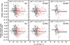 |
Fig. 1. Hubble residuals as a function of Si IIλ6355 velocity (vSi). Top Left: Hubble residuals for NV (black points) and HV (red points) including all redshift sources (see: Section 2.1 for the redshift sources). Top Middle: Same as on the left, but without the template-matched redshift sources. Top right: Same as on the left, but with the template-matched redshift sources alone. Bottom left: Hubble residuals with broken alpha from Ginolin et al. (2025b) for all redshift sources included in the sample. Bottom middle: Same as on the bottom left, but without the template-matched redshift sources. Bottom right: Same as on the bottom left, but with the template-matched redshift sources alone. In all panels, the horizontal black and red lines represent the weighted mean of the Hubble residuals in the NV and HV bins, respectively, where the shaded regions shows the 1σ uncertainty of the weighted means. The vertical dashed grey line represents the criterion (vSi = 12, 000 km s−1) that we used to separate the HV and NV SN Ia samples. The difference of the weighted averages of the HV and NV samples, along with the significances, are shown in each panel. |
We studied the effect of only including SNe Ia with host galaxy redshifts (middle panels) and also including SN template-matched redshift sources (left panels). We also show the sample with the template-matched redshift sources alone (right panel) to clearly show its effect on the combined sample. Given this, a redshift scatter of σz = 10−3 at the mean redshift (z = 0.05) of the 65 SNe Ia in our sample with SNID-based redshifts corresponds to a scatter of ∼285 km s−1 in velocity. This is comparable to or smaller than our Si II line-fit uncertainties. Typically, including SNe with template-matched redshifts alone increases the sample size in lower-mass hosts (Burgaz et al. 2025b).
We first compared the weighted-average Hubble residuals between HV and NV SNe Ia. For all redshift sources, we found a difference in the HR residuals of 0.053 ± 0.024 mag (2.2σ), and without the template-matched sources, the difference was 0.027 ± 0.026 mag (1σ; Fig. 1). The broken-α of Ginolin et al. (2025b) increased these differences to 0.089 ± 0.024 mag (3.7σ) and 0.058 ± 0.027 mag (2.1σ) for the same two samples, respectively. For completeness, we also show the subsample with template-matched redshifts alone. The differences are 0.138 ± 0.056 mag (2.5σ) without broken-α and 0.188 ± 0.057 mag (3.3σ) with broken-α standardisation.
Following Siebert et al. (2020), whose sample within four days of maximum light was divided at the median Si II λ6355 velocity (11,000 km s−1), we tested the differences in HR splitting at the median velocity (11,300 km s−1) for our sample (still defined within four days of maximum light). Using host-galaxy spectroscopic redshifts alone, as Siebert et al. (2020), we found a HR step between NV and HV of 0.052 ± 0.024 mag (2.2σ) without broken-α, and 0.076 ± 0.024 mag (3.1σ) with the broken-α standardisation. When we additionally included SNe with template-matched redshifts in our sample, the HR step increased slightly to 0.073 ± 0.021 mag (3.6σ) and 0.095 ± 0.021 mag (4.5σ). Hence, our separation at 12,000 km s−1 for the HV–NV division and the 11,300 km s−1 split adapted from the method of Siebert et al. (2020) yield HR step measurements that are statistically consistent within 1σ, regardless of the selected redshift source.
Similar to previous analyses, all studied cases showed negative weighted averages for the HV SNe Ia, while the weighted averages of the NV SNe Ia were always positive. SNe Ia with template-matched redshifts in both cases (with or without the broken-α standardisation) increased the significance of the velocity step. These are small significance differences, however, and only the velocity step using the broken-α is significant at 3.7σ (bottom left panel of Fig. 1). Lastly, quite similar to the results of Dettman et al. (2021), the difference of 240 ± 150 km s−1 in the mean Si IIλ6355 velocities between the positive and negative HR samples is insignificant.
3.1.1. Splits by SALT2 light-curve parameters
Our sample is considerably larger than previous samples, and we therefore split the HV and NV SNe Ia according to high-low x1, c, dDLR, host stellar mass, and global and local g–z colour and investigated possible mechanisms that drive the potential differences shown in Fig. 1. In the top left panel of Fig. 2, we firstly compare the HRs without a broken-α standardisation of the low x1 (x1 < 0, blue points) and high x1 (x1 > 0, red points) samples as a function of Si II velocity. The difference between the HRs of the samples when splitting at 12,000 km s−1 (Table 2) is not significant. No significant difference is seen when the broken-α HRs are used (third row, left panel of Fig. 2). We then examined the low- and high-x1 samples of HV and NV SNe Ia separately. Within the NV SNe Ia (comparison between blue and red points at low velocity), the difference is ∼4σ in weighted HR when split by x1. This trend is slightly weaker for HR with the broken alpha, but still above 3σ significance. No significant difference in HR is seen within the HV sample. This trend in the NV sample is likely due to a remaining correlation between HR and x1 that is also seen when the sample is not split by velocity (Ginolin et al. 2025b). It is likely not seen in the HV sample because the sample size is smaller than that of the NV sample.
Weighted averages and significances of the Hubble residuals for the HV and NV samples for different parameters.
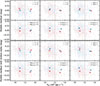 |
Fig. 2. Hubble residuals without (top two rows) and with (bottom two rows) the broken-α standardisation of HV and NV SNe Ia are shown as a function of Si IIλ6355 velocity (all redshift sources included), separated by low and high values of x1, c, dDLR, host galaxy mass, global colour, and local colour. In each plot, the weighted averages (corresponding to high and low values of the parameter) for HV and NV SNe Ia are shown as stars. The vertical dashed line represents the criterion (vSi = 12, 000 km s−1) we used to separate the HV and NV SN Ia samples. To highlight the relative offsets, the panels show a zoomed-in view of the Hubble residuals. The full-scale version is provided in Appendix A. |
The SALT2 c parameter shows no significant trend (all < 3σ) between the HV and NV samples with or without the broken-α standardisation, nor within the HV and NV samples separately for the HR without broken-α standardisation. A difference of 3.9σ arises between the weighted-average HR of the low c NV sample and the high c NV sample using the broken-α standardisation (Table 2).
3.1.2. Splits by host-galaxy parameters
Within the NV sample, the difference is 3.2σ in HR between the low- and high-dDLR subsets for the broken-α standardisation, while the HV sample shows no significant trend with either method. This behaviour is similar to the SALT2 c split, where a HR difference was present in the NV sample, but not in the HV sample. The combined HV and NV sample also showed no trend when split at dDLR = 1, consistent with previous studies (Galbany et al. 2012; Toy et al. 2025).
For the host-mass split (Fig. 2, bottom left panel), the low-mass NV and HV samples show differences in their weighted-average HRs, with significances of 3.1σ (with broken-α) and 3.8σ (without broken-α). The high-mass samples, on the other hand, show no significance for either standardisation models. Within the NV sample, the trend between low- and high-mass hosts is strong, with mass steps of 6.3σ (without broken-α) and 6.6σ (with broken-α). By contrast, the HV sample shows no significant difference for either standardisation.
Similar to host galaxy mass, global colour (Fig. 2, bottom middle panel) shows strong HR trends in the NV sample, with significances of 5.9σ (without broken-α) and 6.9σ (with broken-α). Unlike the mass, the HV sample also shows a trend at 3–4σ between the low- and high-colour subsets. No significant differences are found between HV and NV at either low or high colour. For local instead of global colour, the results are consistent with slightly higher significances (Table 2).
3.1.3. Summary of the parameter splits
As summarised in Table 2, for the HRs as a function of velocity, the differences within the NV subsample without broken-α standardisation are significant when we split the sample for x1, as well as for the host parameters of stellar mass, and local and global colours. All of the parameters (SN Ia and host galaxy light curves) we investigated are significantly different in HRs within the NV subsample when the broken-α formulation is considered. We considered the stellar mass, and the local and global colours have the most robust significant HR differences with the NV sample because they are seen without and with broken-α standardisation at > 5.9 σ.
For the non-broken-α and broken-α analyses, the significances in the HRs are not as significant for the HV subsample for the global and local galaxy colour (Table 2), and there is no significant difference for global mass. Since a significant difference in HRs is seen in the NV and HV samples (although it is lower for the HV sample) for the global and local colour, this suggests that the velocities measured at peak in SNe Ia do not drive this HRs difference. It would otherwise be seen in just one of the samples. The difference in HRs with the NV sample is very significant at > 6σ for the host stellar mass, however, but a no difference in HRs within the NV sample is seen, suggesting that the host stellar mass might be more closely linked to the SN velocity.
We chose to use a velocity of 12,000 km s−1 to split our sample, following Burgaz et al. (2025a). The exact velocity used for this split is somewhat arbitrary, however, with other studies employing values of 11,800 km s−1 or 12,000 km s−1. Different phase definitions and different sub-classification selections have also been used. In Appendix A we show the results from our sample when the velocity separation is taken as 11,800 km s−1 and present an analysis with transitional subclasses near the normal subtype, such as 99aa-like and 04gs-like SNe Ia included to investigate the sample selection effect. We finally investigate the phase-selection effect by applying a stricter phase cut (within 3 d of peak) on our sample in Appendix A. A lower velocity separation threshold from 12,000 km s−1 to 11,800 km s−1 slightly enhances the significance levels for normal SNe Ia alone. This increase in significance becomes negligible when 99aa-like and 04gs-like SNe are incorporated in the sample, however.
3.2. Host mass and colour steps
Ginolin et al. (2025b) demonstrated a larger HR mass step in stretch standardisation by introducing a broken-α model compared to a standard alpha model. This was complemented by Ginolin et al. (2025a), focusing on SN Ia colour and dust, to explore colour standardisation. We investigated the global host-mass step separately for HV and NV SNe Ia.
The left panels of Fig. 3 show that only the NV SNe Ia show a significant global mass step when the sample is split at log(M★/M⊙) = 10, while HV SNe Ia step amplitudes are much lower and are not statistically distinguished from zero (i.e. ≲2σ), both without and with a broken-α standardisation. For NV events, we measured steps of 0.149 ± 0.024 mag (6.3σ) without broken-α standardisation and steps of 0.161 ± 0.025 mag (6.6σ) with broken-α standardisation. In contrast, HV SNe Ia mass steps are 0.046 ± 0.041 mag (1.1σ) and 0.077 ± 0.042 mag (1.9σ) under the two standardisations, respectively. The difference between the NV and HV mass steps corresponds to 0.103 mag (2.2σ) without broken-α and 0.083 mag (1.7σ) with broken-α, respectively. A velocity separation of 11,800 km s−1 instead of 12,000 km s−1 yields slightly higher significances for the NV–HV mass-step difference, with values of 0.115 mag (2.6σ) without broken-α standardisation and 0.087 mag (1.9σ) with broken-α. The effect of the velocity cut choice is investigated further in Appendix A.
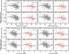 |
Fig. 3. Hubble residuals as a function of global and local host galaxy mass (top two rows). The top row of plots displays the Hubble residuals without the broken-α standardisation, and the bottom row shows the Hubble residuals with it. In each plot, black circles represent NV SNe Ia, and red circles represent HV SNe Ia. The horizontal black and red lines show the weighted averages of the Hubble residuals for the NV and HV samples, respectively, and the shaded regions represent the 1σ uncertainties of these averages. The vertical dashed lines at log(M★/M⊙) = 10 show the division between low- and high-mass samples based on global host galaxy mass in the left panels, and the dashed lines at log(M★/M⊙) = 8.9 show the division based on local host galaxy mass in the right panels. The difference in the weighted averages between the low- and high-mass samples, along with the corresponding significances, are shown in each panel. The Hubble residuals as a function of global and local g–z colours are shown in the bottom two rows. The vertical dashed line represents the criterion (g–z = 1) we used to separate the low- and high-colour environments. |
We also repeated the analysis using local instead of global host galaxy masses (right panels of Fig. 3). The NV SNe Ia again show a significant local mass step of 0.141 ± 0.024 mag (5.9σ) without broken-α standardisation and steps of 0.177 ± 0.025 mag (7.2σ) with broken-α. In contrast, HV SNe Ia again show a much smaller amplitudes with values of 0.064 ± 0.041 mag (1.6σ) and 0.089 ± 0.042 mag (2.1σ), respectively, and are not statistically distinguished from zero.
Considering the differences in sample sizes, we tested the robustness of the observed mass step by randomly selecting 70 NV SNe Ia (from the original 207) to match the number of HV SNe Ia. The random draws were weighted to reproduce the same low- and high-mass host proportions as in the HV sample. After 105 resamplings, only 0.1% of realisations yield a mass step with a significance equal to or smaller than that observed in the HV sample (1.1σ) without the broken-α standardisation, with a mean significance of 3.6σ. The same analysis with the broken-α standardisation gives a consistent result: 0.3% of realisations fall below the HV value (1.9σ), with a mean significance of 3.8σ. These tests indicate that the weaker HV mass step cannot be explained by the smaller sample size, which supports the conclusion that the mass-step amplitudes are significantly reduced (resulting in significances that are not statistically distinguished from zero) in HV SNe Ia.
We also investigated the dependence of SN Ia HRs on the global rest-frame g–z colour of their host galaxies. In Fig. 3 we show the HRs versus the host rest-frame g–z colour split at g–z = 1. The NV SNe Ia show a host-colour HR step of 0.142 ± 0.024 mag (5.9σ) and 0.168 ± 0.025 mag (6.8σ) without and with broken-α standardisation, respectively. In contrast to the host galaxy mass, the HV SNe Ia also show a significant step of 0.158 ± 0.042 mag (3.8σ) without broken-α, and 0.168 ± 0.043 mag (4σ) with broken-α. The NV and HV colour steps are statistically consistent.
We also repeated the analysis using the local rest-frame g–z colour instead of the global colour. For NV SNe Ia, the step size is similar, but the significance is slightly higher, with values of 0.147 ± 0.024 mag (6.2σ) without broken-α and 0.170 ± 0.025 mag (6.9σ) with broken-α. For HV SNe Ia, the size and significance of the step both decrease compared to the global colour, with values of 0.129 ± 0.041 mag (3.1σ) without broken-α and 0.137 ± 0.042 mag (3.3σ) with broken-α.
3.3. HRs for host mass/colour and dDLR
dDLR measures the SN to host offset in units of the directional host light radius along the SN direction, which means that dDLR < 1 selects events within roughly one light radius (inner disk/bulge), whereas dDLR > 1 selects events in the outer disk, outskirts, or low surface brightness features. The inner regions have a higher stellar-mass density and metallicity on average and a more homogeneously distributed dust component. The outer regions, on the other hand, have a lower average metallicity and highly clumpy distribution of dust on average, with patchy star-forming regions that can produce localised extinction. If SN Ia subpopulations track the progenitor metallicity, age, or dust geometry, a different Hubble-residual behaviour between the dDLR < 1 and dDLR > 1 regimes might arise.
Figure 4 shows the HRs (again without and with broken-α standarisation) as a function of global mass split into those with dDLR < 1 and those with dDLR > 1. For small dDLR, the NV sample shows a global mass step with a significance at 6.5σ and a step of 0.165 ± 0.025 mag without broken-α standardisation. No significant step is observed for dDLR > 1 for NV SNe Ia, nor for the HV SNe Ia sample at small or large dDLR. Toy et al. (2025) showed that the overall size of the stellar mass step (not split into NV and HV SNe Ia) depends on the galactocentric distance, where for dDLR < 1, a significance of 6.9σ with a mass step of 0.100 ± 0.014 mag was observed. No significant step was observed for dDLR > 1. Our result of a mass step for the NV of 0.165 ± 0.025 mag (6.5σ) is consistent with this, but we additionally find that the size of the step increases when only considering the NV events, suggesting that the mass step for dDLR < 1 might be specifically driven by NV SNe Ia.
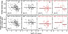 |
Fig. 4. Hubble residual plots without and with the broken alpha standardisation as a function of host galaxy mass for HV and NV SNe Ia split by dDLR. The black and red dots represent the NV and HV SNe Ia, respectively. The vertical dashed line represents the criterion (log(M★/M⊙) = 10 for the global mass samples). In each plot, the horizontal dashed lines represent the weighted mean of the Hubble residuals, and the shaded regions shows the 1σ uncertainty of the weighted means. The difference of the weighted averages between the low- and high-mass samples along with the significances are shown in the label. |
We repeated the analysis of the samples split by dDLR with respect to global colour of the host galaxies instead of mass and show this in Fig. 5. Following Kelsey et al. (2021, 2023), Toy et al. (2025) showed that the host galaxy rest-frame U–R colour split at 1 shows a significant step for the dDLR < 1 sample alone. Our findings agree with this, where we find a 5.1σ significance with 0.131 ± 0.026 step for NV SNe Ia for the dDLR < 1 sample in our host galaxy rest-frame g–z analysis. Interestingly, HV SNe Ia also show a weak trend for the dDLR < 1 subsample with a significance of 3.0σ for the colour, where no significant mass step was seen for this sample.
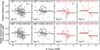 |
Fig. 5. Same as Fig. 4, but as a function of global colour (g–z) for HV and NV SNe Ia split by dDLR. The vertical dashed line represents the criterion (g–z = 1) we used to separate the global low- and high-colour samples. |
To further quantify the differences observed in the low- and high-dDLR samples, we performed KS tests that compared NV and HV SNe Ia within each sub-sample separately. For the low- dDLR sample, there is no strong evidence that the distributions of global and local galaxy mass, global and local rest-frame colour, or SALT2 x1 differ between NV and HV SNe Ia. In this low- dDLR subsample, the SALT2 c parameter differs between NV and HV SNe Ia, however, with a p-value of 0.0156. This indicates that HV SNe Ia tend to be redder than NV SNe Ia. Similarly, for the high-dDLR sample, there is no significant difference between NV and HV SNe Ia for global and local galaxy mass, global and local colour, or x1, but the SALT2 c parameter also shows a significant difference (p-value = 0.0176), which again suggests redder colours for HV SNe Ia. These results are consistent with previously reported trends for HV and NV SNe Ia in terms of the SALT2 c parameter (Wang et al. 2013; Burgaz et al. 2025a).
4. Discussion
We have investigated the relation between SN Ia HRs obtained from light-curve fits to the ZTF SN Ia sample and the intrinsic Si II 6355 velocities measured from SN Ia spectra around maximum light. We also investigated the connection between the extrinsic host galaxy mass or colour HR step and the intrinsic Si II velocities of the SNe Ia.
4.1. A mass step driven by the NV sample
A key result is that we identified strong mass steps of 0.141–0.177 mag at 6–7σ significance in the NV sample, depending on whether local or global masses or a standardisation without or with broken alpha are included. For the HV sample, the corresponding steps are smaller (0.046–0.089 mag) and of low significance. The difference between the global NV and HV mass steps is at a modest significance of ∼2.2σ without broken-α and ∼1.7σ with broken-α. While the global NV–HV difference is only marginally significant, the stronger NV trend compared to HV might indicate that the origin of the mass step might be at least partly connected to intrinsic SN Ia properties, such as the explosion velocity, as measured here.
Similar colour steps of 0.142–0.170 mag exist at 6–7σ significance for the NV sample. The HV sample also shows colour steps of 0.129–0.168 mag, with a lower significance (2.5–3.8σ) that might be due to the smaller sample size, but the NV and HV colour steps are statistically consistent. This might suggest that the mass step is driven by something more intrinsic to the SNe Ia than the colour step because it is seen only for NV SNe, and that the colour of the SN environment at the time of explosion is less directly related to the origin of the diversity of SN Ia velocities.
The colour step but not a mass step for the HV has a subtle reason and is driven by small numbers of SNe Ia moving from high mass to blue or red colour to low mass. This causes them to switch from one side of the step to the other. For reference, the NV counts are 28 (low-mass red), 75 (low-mass blue), 82 (high-mass red), and 22 (high-mass blue), while the corresponding HV counts are 8, 26, 34, and 2, respectively (Fig. 6). In three quadrants (low-mass red, low-mass blue, and high-mass red), the HV-to-NV ratio is consistently ∼1:3, but the high-mass blue bin only contains two HV events. Under the assumption of a uniform HV fraction, we would expect 7.4 ± 2.7 HV SNe Ia in this bin, corresponding to a difference of ∼2σ from the observed number of two SNe. This suggests that HV SNe Ia might be less common in high-mass blue galaxies. The statistical significance is only modest, however, and larger samples are required to confirm this effect. Therefore, it is difficult to determine the reason for the differences in the amplitudes and significances of the mass and colour steps.
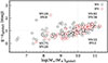 |
Fig. 6. Distribution of NV and HV SNe Ia across host galaxy mass and global colour. HV and NV SNe Ia are represented with red and black circles, respectively. The vertical dashed line at log(M★/M⊙) = 10 marks the division between low- and high-mass galaxies, and the horizontal dotted line at g–z = 1 marks the division between blue and red hosts. |
Given the size of the volume-limited ZTF DR2 sample and the inclusion of SNe Ia in host galaxies without spectroscopic redshifts, it contains more SNe Ia in low-mass host galaxies than previous samples. Burgaz et al. (2025b) ran a series of analyses on HV SNe Ia in low-mass galaxies and found that the occurrence rate was similar to that of NV SNe Ia. This was an update to previous results that suggested a higher occurrence in high-mass hosts that was likely due to sample biases. In this analysis, only one HV SNe Ia has a host galaxy mass, log(M★/M⊙), lower than 8, while there are 12 NV SNe Ia. To test how these SNe Ia in the lowest-mass hosts might affect our results, we removed the SNe Ia with log(M★/M⊙) < 8, which dropped the mass step to 0.136 ± 0.025 mag (5.5σ) for NV SNe Ia, but the step still remained significant. Since the significance change is around 0.7σ, a similar increase in HV SNe Ia, if they had the same number of objects in the log(M★/M⊙) < 8 area would still result in a significance lower than 2σ.
For the mass step when the ZTF SN Ia sample was split into HV and NV samples, the difference appears to be driven by a shift in the mean HR in low-mass galaxies towards a more positive value for NV SNe, with both the NV and HV SNe in high-mass galaxies having similar HRs, regardless of the use of the broken-α standardisation, or global or local stellar mass. For the HRs with respect to galaxy colour, the mean HR for NV SNe in blue and red galaxies is similar to that of NV SNe in low- and high-mass galaxies, respectively. For HV SNe, the appearance of a colour step, where no global mass step is seen, is driven by a shift towards more positive HRs in blue galaxies and towards more negative HRs in red galaxies. These HV shifts correspond to modest (∼2.5–3.8σ) detections, which are not drastically different in significance from NV results in certain bins. As discussed by Burgaz et al. (2025a), there is a small difference in the underlying SALT2 x1 and c distributions of the NV and HV samples, with the HV sample having marginally narrower light curves and redder colours on average. Wang et al. (2013) showed for a sample of SNe Ia from the galaxy-targeted Lick Observatory Supernova Search that HV SNe Ia preferentially resided in the inner regions of their host galaxies, as measured by the semi-major axis at the 25 mag arcsec2 isophote in the B band. This is not seen in this untargeted ZTF SN Ia sample, however, where the ratio is constant at ∼30% HV to NV up to a dDLR of ∼2 (Burgaz et al. 2025b). The dDLR corrects for the effect of inclination, which is not accounted for when using the semi-major axis, which along with the targeted versus untargeted nature of the survey likely explains the differences in the results.
4.2. Connection to the galactocentric distance of the host galaxy
We also compared SNe Ia with different peak velocities in the central regions of their hosts (dDLR < 1) and those in the outskirts (dDLR > 1). We confirmed the relation between mass step and dDLR of Toy et al. (2025), but we further showed that this relation is driven by the NV SNe Ia, with a strong and statistically significant mass step of 0.165 ± 0.025 mag (6.5σ) for the NV sample at small dDLR. In contrast, when NV SNe occur in galaxy outskirts (dDLR > 1), the mass step disappears entirely. A similar trend emerges for the global and local host rest-frame colour (g–z), where NV SNe show a 5σ colour step at dDLR < 1, but no significant step in the outskirts.
For HV SNe Ia, the central-region mass step is consistent with zero (−0.021 ± 0.027 mag). This yields a NV–HV contrast of 3.1–3.6σ, representing the most significant subtype difference we find. HV SNe exhibit non-zero steps of ∼0.18–0.21 mag in the outskirts, however, with a significance of 2.6–2.9σ. This suggests for HV SNe Ia that while the residuals of their luminosities are not affected by stellar mass, they might still retain some sensitivity to the local stellar population age, metallicity, or dust content, as traced by host colour (Ginolin et al. 2025b). The fact that a weak colour step exists in the inner and outer regions of the host galaxies of HV SNe (although it is less pronounced than for NV SN samples at small dDLR) suggests that HRs of HV SNe are subtly linked to their galaxy colours, but this is relatively independent of dDLR.
The properties of galaxies as a function of radial distance were investigated, and the identified trends depend on the galaxy type. For early-type/elliptical and late-type/spiral galaxies, the stellar metallicity was found to decrease slightly with increasing radial distance (González Delgado et al. 2015; Goddard et al. 2017). The dependence of the stellar ages on the radial distances is different in different galaxy types, however. Stars in the outer regions of early-type galaxies are likely the same or only marginally older than stars in the inner regions (Goddard et al. 2017). In late-type galaxies, the inner regions that are dominated by bulges are likely older than the outer regions. Dust gradients also exist within galaxies, with all galaxy types showing increased extinction due to dust towards their centres (González Delgado et al. 2015; Goddard et al. 2017), and several studies have proposed that dust might contribute significantly to the mass step (Brout & Scolnic 2021; Popovic et al. 2023). Toy et al. (2025) investigated the difference in the mass step they observed between inner and outer regions of their host galaxies, however, and found that varying total-to-selective extinction, RV was insufficient to explain it. Therefore, it remains an open question what drives these relations. That the galaxy steps sizes differ when the sample is split based on intrinsic velocity of the SN ejecta and the distance from the centre of the host galaxy suggests, however, that the origin must be at least somewhat intrinsic to the SN and dependent on the progenitor scenario or on the specifics of the explosion mechanism.
4.3. The connection between galaxy HR steps and intrinsic SN properties
Our findings imply that the widely reported HR steps with host galaxy mass and colour are not universal for all SNe Ia, but instead depend strongly on at least one intrinsic property of SNe Ia, their explosion velocities as measured at peak. Although the overall difference in the mass step between NV and HV SNe Ia is only marginal (∼2.2σ), the evidence of a subtype dependence is stronger for SNe that are located in the central regions of their hosts (dDLR < 1), where the contrast reaches 3.1–3.6σ. Moreover, the way in which the mass and colour steps vary with galactocentric distance differs between the two velocity subtypes. Hence, the subtype and location dependence raises the possibility that dust is not the sole driver of the mass and colour steps. Additional factors such as intrinsic SN Ia properties or local environments may play a role, and correlations between progenitor age, dust properties, and explosion velocity might also contribute.
The HV SNe appear to more uniform across a range of stellar masses and colours, but still show modest (∼2.5–3σ) steps in some bins, while the luminosities of the NV SNe show a dependence on both mass and colour. Previous studies such as Rigault et al. (2013) and Childress et al. (2013) suggested that the mass/colour step might be caused by differences in the luminosity of SNe Ia from young and old populations or two different progenitor channels that have different mean ages and luminosities. Wiseman et al. (2023) suggested, however, that it is likely that a luminosity step with progenitor age, as well as a total-to-selective dust extinction ratio, RV, that changes with galaxy age, drives the differences in HR residuals in different galaxy environments. Our results agree with Wiseman et al. (2023) and show indicationss of intrinsic differences between HV and NV SNe Ia. If this is the case, the contrast might be linked to the progenitor age together with dust effects, and it might include different dust laws for the two subtypes.
A completely intrinsic origin for the galaxy steps cannot be ruled out, however, because if, for example, there were subtle metallicity differences in the progenitor stars (due to different birth environments), then this might cause differences in the observed properties of the SNe Ia and hence the HRs. This has been suggested theoretically even within specific explosion scenarios, such as the double-detonations of sub-Chandrasekhar mass white dwarfs where differences in nucleosynthetic yields are seen when just the metallicity is varied (e.g., Shen et al. 2018; Leung & Nomoto 2020; Gronow et al. 2021). While these studies did not directly predict Hubble residuals, these luminosity shifts would appear as residual offsets after standardisation if present in real populations, as also suggested by observational trends between metallicity and HRs (e.g., Childress et al. 2013; Pan et al. 2014).
The way in which NV and HV SNe Ia respond differently to their environments might alternatively indicate that they come from different progenitor systems or explosion mechanisms. The strong correlation between HRs and local host properties for NV SNe, particularly in central, metal-rich, and older stellar populations, indicates a scenario in which NV SNe preferentially originate from older progenitor systems with a higher metallicity. This is consistent with a longer time until explosion for the progenitor scenario (e.g. double-degenerate systems or single-degenerate systems with longer delay times), where the progenitor white dwarf(s) evolve in environments shaped by metallicity and age (e.g., Liu et al. 2023). The relatively weak or completely absent environmental dependence for HV SNe, especially the lack of a mass step at any galactocentric radius, implies that their progenitor systems might be more uniform and/or possibly younger, however. This arises from a different or less environment-sensitive channel. This might reflect a preference for either a star-forming or an intermediate-age environment, or a lower metallicity.
For NV SNe, global host properties only predict SN luminosity residuals when the SN arises from the central galaxy region, supporting a local-environment origin of the mass and colour step. For HV SNe, environmental trends are weaker, but not always absent, and some subsets show non-zero steps at a modest significance, which might reflect intrinsic differences between NV and HV SNe Ia, such as variations in the progenitor channels or explosion physics.
These results highlight the importance of incorporating local environmental context and spectroscopic information in SNe Ia standardisation for precision cosmology.
5. Conclusions
Based on the spectroscopically classified SNe Ia from the volume-limited sample of ZTF DR2 at peak light, we analysed the NV and HV SNe Ia through their HRs and studied the effect of light-curve parameters and host galaxy separation on the estimated mass and colour steps. The main conclusions are listed below.
-
HV and NV SNe Ia show no significant differences in HRs in most cases. In the specific case of a broken-α standardisation and when all redshift sources are included, however, a significance of 3.7σ was found. Excluding template-matched redshifts reduces significance, suggesting that the selection of redshift sources and sample size affect the results.
-
Significant trends in HR were found within the NV SNe Ia sample when split by x1, c, host mass, dDLR, and local/global environment properties when using broken-α standardisation. The strongest trends reached up to 6.9σ for environmental colour. HV SNe Ia show weaker internal trends overall, but do exhibit modest signals (typically ∼2.5–3σ) in some subsets, including local/global colour and outer regions.
-
We found a highly significant (6.3σ) mass step in NV SNe Ia, while HV SNe Ia show no significant mass step. Quantitatively, the global NV and HV mass steps differ at a modest difference of ∼2.2σ (no broken-α) or ∼1.7σ (broken-α).
-
We observed a 0.142 ± 0.024 mag (5.9σ) colour step in NV SNe Ia and a 0.158 ± 0.042 mag (3.8σ) colour step in HV SNe Ia. Even though the HV SNe Ia colour step is larger, its significance appears to be modest, possibly due to the smaller sample size. The NV and HV colour steps are statistically consistent overall.
-
The mass step is present only for NV SNe Ia located near the centres of their host galaxies (dDLR). For NV SNe in the outskirts, the mass step disappears entirely. On the other hand, HV SNe Ia show no central-region mass step, but display larger steps (∼0.18–0.21 mag) at ∼2.6–2.9σ in the outer regions. The most significant subtype difference occurs for central events (dDLR < 1), where NV show a mass step, while HV are consistent with none, corresponding to a difference of 3.1–3.6σ between the two subtypes.
-
A KS test showed that HV and NV SNe Ia located near galaxy centres (dDLR < 1) differ in SALT2 colour (c), with HV SNe showing redder values. This supports the idea that HV SNe are either dustier or have intrinsically different colours, which is consistent with differences in progenitor systems or explosion mechanisms.
-
A similarly strong dependence on the host rest-frame global colour (g–z) is observed for NV SNe only when the SNe occur in the central regions of the galaxy are considered, suggesting that this might be driven by local stellar population properties, such as metallicity, age, or dust, and not by global host mass or colour. We therefore emphasize central environments as the likely drivers of the NV trend.
-
HV SNe Ia show a modest host galaxy colour step in the central and outer regions (3.0σ and 2.4σ, respectively), which suggests a possible sensitivity to the progenitor age or dust, but the sensitivity is not sufficiently strong to be used as a reliable correction. These results are statistically consistent with the NV colour steps.
The different response of NV and HV SNe Ia to the host galaxy environment suggests a strong connection between the intrinsic properties of the SN explosion (e.g. explosion energy) and the environments within which the SNe Ia were born or explode. Because the global NV–HV mass-step difference is at a modest ∼2.2σ, however, our interpretation primarily relies on the stronger central region result (3.1–3.6σ). We find a strong correlation between Hubble residuals and host properties for NV SNe, particularly in central likely metal-rich and older stellar populations. This suggests that while NV SNe Ia are environmentally sensitive, HV SNe Ia are not, possibly because they represent a more homogeneous population.
Our results imply that SNe Ia standardisation needs to account for the spectroscopic subtype and for the local environment. A uniform application of mass or colour steps may introduce systematic errors if these variables are not carefully considered. We recommend reporting the measured steps with their uncertainties for each subtype and galactocentric bin and adopting subtype- and location-aware corrections (e.g., dDLR-weighted) instead of a single universal step. The correlation between global host mass and SN luminosity residuals is strongest when the SN is located near the galaxy centre. This suggests that the host galaxy properties might not be equally informative at all galactocentric distances. This reinforces the value of spatially resolved environmental metrics in future cosmological surveys. In future SN Ia cosmology analyses that incorporate local photometry and/or spectroscopy and SN subtype, the scatter in precision cosmology might be significantly improved. In particular, spatially resolved spectroscopy to constrain environmental properties such as metallicity and stellar population age might help us clarify the role of the host environment, while the galactocentric distance might serve as a useful weighting factor in the SN standardisation to reduce residual scatter.
Acknowledgments
Based on observations obtained with the Samuel Oschin Telescope 48-inch and the 60-inch Telescope at the Palomar Observatory as part of the Zwicky Transient Facility project. ZTF is supported by the National Science Foundation under Grants No. AST-1440341 and AST-2034437 and a collaboration including current partners Caltech, IPAC, the Weizmann Institute of Science, the Oskar Klein Center at Stockholm University, the University of Maryland, Deutsches Elektronen-Synchrotron and Humboldt University, the TANGO Consortium of Taiwan, the University of Wisconsin at Milwaukee, Trinity College Dublin, Lawrence Livermore National Laboratories, IN2P3, University of Warwick, Ruhr University Bochum, Northwestern University and former partners the University of Washington, Los Alamos National Laboratories, and Lawrence Berkeley National Laboratories. Operations are conducted by COO, IPAC, and UW. SED Machine is based upon work supported by the National Science Foundation under Grant No. 1106171. U.B, K.M., and T.E.M.B. are funded by Horizon Europe ERC grant no. 101125877. JHT is supported by the H2020 European Research Council grant no. 758638. L.G. acknowledges financial support from AGAUR, CSIC, MCIN and AEI 10.13039/501100011033 under projects PID2023-151307NB-I00, PIE 20215AT016, CEX2020-001058-M, ILINK23001, COOPB2304, and 2021-SGR-01270. This project has received funding from the European Research Council (ERC) under the European Union’s Horizon 2020 research and innovation program (grant agreement n 759194 - USNAC). Y.-L.K. was supported by the Lee Wonchul Fellowship, funded through the BK21 Fostering Outstanding Universities for Research (FOUR) Program (grant No. 4120200513819) and the National Research Foundation of Korea to the Center for Galaxy Evolution Research (RS-2022-NR070872, RS-2022-NR070525). This research used resources of the National Energy Research Scientific Computing Center (NERSC), a Department of Energy User Facility using NERSC award HEP-ERCAP0033784. This work has been supported by the research project grant “Understanding the Dynamic Universe” funded by the Knut and Alice Wallenberg Foundation under Dnr KAW 2018.0067. AG acknowledges support from Vetenskapsrådet, the Swedish Research Council, project 2020-03444, as well as the Swedish National Space Agency, under Dnr 2023-00226. NR is supported by DoE award #DE-SC0025599. Zwicky Transient Facility access for NR was supported by Northwestern University and the Center for Interdisciplinary Exploration and Research in Astrophysics (CIERA)
References
- Abdurro’uf, Accetta, K., Aerts, C., et al. 2022, ApJS, 259, 35 [NASA ADS] [CrossRef] [Google Scholar]
- Amenouche, M., Rosnet, P., Smith, M., et al. 2025, A&A, 694, A3 [NASA ADS] [CrossRef] [EDP Sciences] [Google Scholar]
- Bellm, E. C., Kulkarni, S. R., Graham, M. J., et al. 2019, PASP, 131, 018002 [Google Scholar]
- Benetti, S., Cappellaro, E., Turatto, M., et al. 2006, ApJ, 653, L129 [NASA ADS] [CrossRef] [Google Scholar]
- Betoule, M., Kessler, R., Guy, J., et al. 2014, A&A, 568, A22 [NASA ADS] [CrossRef] [EDP Sciences] [Google Scholar]
- Blagorodnova, N., Neill, J. D., Walters, R., et al. 2018, PASP, 130, 035003 [Google Scholar]
- Blondin, S., & Tonry, J. L. 2007, ApJ, 666, 1024 [NASA ADS] [CrossRef] [Google Scholar]
- Branch, D., & Miller, D. L. 1993, ApJ, 405, L5 [Google Scholar]
- Brout, D., & Scolnic, D. 2021, ApJ, 909, 26 [NASA ADS] [CrossRef] [Google Scholar]
- Brout, D., Scolnic, D., Popovic, B., et al. 2022, ApJ, 938, 110 [NASA ADS] [CrossRef] [Google Scholar]
- Burgaz, U., Maeda, K., Kalomeni, B., et al. 2021, MNRAS, 502, 4112 [NASA ADS] [CrossRef] [Google Scholar]
- Burgaz, U., Maguire, K., Dimitriadis, G., et al. 2025a, A&A, 694, A9 [NASA ADS] [CrossRef] [EDP Sciences] [Google Scholar]
- Burgaz, U., Maguire, K., Dimitriadis, G., et al. 2025b, A&A, 694, A13 [NASA ADS] [CrossRef] [EDP Sciences] [Google Scholar]
- Burns, C. R., Stritzinger, M., Phillips, M. M., et al. 2011, AJ, 141, 19 [Google Scholar]
- Burns, C. R., Stritzinger, M., Phillips, M. M., et al. 2014, ApJ, 789, 32 [Google Scholar]
- Chakraborty, S., Sadler, B., Hoeflich, P., et al. 2024, ApJ, 969, 80 [NASA ADS] [CrossRef] [Google Scholar]
- Chambers, K. C., Magnier, E. A., Metcalfe, N., et al. 2016, arXiv e-prints [arXiv:1612.05560] [Google Scholar]
- Childress, M., Aldering, G., Antilogus, P., et al. 2013, ApJ, 770, 108 [Google Scholar]
- Chung, C., Yoon, S.-J., Park, S., et al. 2023, ApJ, 959, 94 [NASA ADS] [CrossRef] [Google Scholar]
- Chung, C., Park, S., Son, J., Cho, H., & Lee, Y.-W. 2025, MNRAS, 538, 3340 [Google Scholar]
- D’Andrea, C. B., Gupta, R. R., Sako, M., et al. 2011, ApJ, 743, 172 [Google Scholar]
- Dekany, R., Smith, R. M., Riddle, R., et al. 2020, PASP, 132, 038001 [NASA ADS] [CrossRef] [Google Scholar]
- DES Collaboration (Abbott, T. M. C., et al.) 2024, ApJ, 973, L14 [NASA ADS] [CrossRef] [Google Scholar]
- Dettman, K. G., Jha, S. W., Dai, M., et al. 2021, ApJ, 923, 267 [NASA ADS] [CrossRef] [Google Scholar]
- Dey, A., Schlegel, D. J., Lang, D., et al. 2019, AJ, 157, 168 [Google Scholar]
- Dimitriadis, G., Burgaz, U., Deckers, M., et al. 2025, A&A, 694, A10 [NASA ADS] [CrossRef] [EDP Sciences] [Google Scholar]
- Filippenko, A. V., Richmond, M. W., Branch, D., et al. 1992a, AJ, 104, 1543 [NASA ADS] [CrossRef] [Google Scholar]
- Filippenko, A. V., Richmond, M. W., Matheson, T., et al. 1992b, ApJ, 384, L15 [CrossRef] [Google Scholar]
- Fink, M., Hillebrandt, W., & Röpke, F. K. 2007, A&A, 476, 1133 [NASA ADS] [CrossRef] [EDP Sciences] [Google Scholar]
- Fioc, M., & Rocca-Volmerange, B. 1997, A&A, 326, 950 [NASA ADS] [Google Scholar]
- Foley, R. J., & Kasen, D. 2011, ApJ, 729, 55 [Google Scholar]
- Freedman, W. L., Madore, B. F., Hatt, D., et al. 2019, ApJ, 882, 34 [Google Scholar]
- Galbany, L., Miquel, R., Östman, L., et al. 2012, ApJ, 755, 125 [NASA ADS] [CrossRef] [Google Scholar]
- Galbany, L., de Jaeger, T., Riess, A. G., et al. 2023, A&A, 679, A95 [NASA ADS] [CrossRef] [EDP Sciences] [Google Scholar]
- Ganeshalingam, M., Li, W., & Filippenko, A. V. 2011, MNRAS, 416, 2607 [NASA ADS] [CrossRef] [Google Scholar]
- Ganeshalingam, M., Li, W., Filippenko, A. V., et al. 2012, ApJ, 751, 142 [NASA ADS] [CrossRef] [Google Scholar]
- Garavini, G., Folatelli, G., Goobar, A., et al. 2004, AJ, 128, 387 [NASA ADS] [CrossRef] [Google Scholar]
- Ginolin, M., Rigault, M., Copin, Y., et al. 2025a, A&A, 694, A4 [NASA ADS] [CrossRef] [EDP Sciences] [Google Scholar]
- Ginolin, M., Rigault, M., Smith, M., et al. 2025b, A&A, 695, A140 [NASA ADS] [CrossRef] [EDP Sciences] [Google Scholar]
- Goddard, D., Thomas, D., Maraston, C., et al. 2017, MNRAS, 466, 4731 [NASA ADS] [Google Scholar]
- González Delgado, R. M., García-Benito, R., Pérez, E., et al. 2015, A&A, 581, A103 [Google Scholar]
- Graham, M. J., Kulkarni, S. R., Bellm, E. C., et al. 2019, PASP, 131, 078001 [Google Scholar]
- Grayling, M., Thorp, S., Mandel, K. S., et al. 2024, MNRAS, 531, 953 [NASA ADS] [CrossRef] [Google Scholar]
- Gronow, S., Côté, B., Lach, F., et al. 2021, A&A, 656, A94 [NASA ADS] [CrossRef] [EDP Sciences] [Google Scholar]
- Gupta, R. R., Kuhlmann, S., Kovacs, E., et al. 2016, AJ, 152, 154 [NASA ADS] [CrossRef] [Google Scholar]
- Guy, J., Astier, P., Baumont, S., et al. 2007, A&A, 466, 11 [NASA ADS] [CrossRef] [EDP Sciences] [Google Scholar]
- Guy, J., Sullivan, M., Conley, A., et al. 2010, A&A, 523, A7 [NASA ADS] [CrossRef] [EDP Sciences] [Google Scholar]
- Hamuy, M., Phillips, M. M., Maza, J., et al. 1995, AJ, 109, 1 [NASA ADS] [CrossRef] [Google Scholar]
- Hayden, B. T., Gupta, R. R., Garnavich, P. M., et al. 2013, ApJ, 764, 191 [Google Scholar]
- Howell, D. A., Sullivan, M., Nugent, P. E., et al. 2006, Nature, 443, 308 [Google Scholar]
- Hoyle, F., & Fowler, W. A. 1960, ApJ, 132, 565 [NASA ADS] [CrossRef] [Google Scholar]
- Iben, I., Jr, & Tutukov, A. V. 1984, ApJS, 54, 335 [NASA ADS] [CrossRef] [Google Scholar]
- Jha, S. W., Maguire, K., & Sullivan, M. 2019, Nat. Astron., 3, 706 [NASA ADS] [CrossRef] [Google Scholar]
- Kelly, P. L., Hicken, M., Burke, D. L., Mandel, K. S., & Kirshner, R. P. 2010, ApJ, 715, 743 [Google Scholar]
- Kelsey, L., Sullivan, M., Smith, M., et al. 2021, MNRAS, 501, 4861 [NASA ADS] [CrossRef] [Google Scholar]
- Kelsey, L., Sullivan, M., Wiseman, P., et al. 2023, MNRAS, 519, 3046 [Google Scholar]
- Kenworthy, W. D., Jones, D. O., Dai, M., et al. 2021, ApJ, 923, 265 [NASA ADS] [CrossRef] [Google Scholar]
- Kim, Y.-L., Smith, M., Sullivan, M., & Lee, Y.-W. 2018, ApJ, 854, 24 [NASA ADS] [CrossRef] [Google Scholar]
- Kim, Y. L., Rigault, M., Neill, J. D., et al. 2022, PASP, 134, 024505 [NASA ADS] [CrossRef] [Google Scholar]
- Kim, Y.-L., Galbany, L., Hook, I., & Kang, Y. 2024, MNRAS, 529, 3806 [CrossRef] [Google Scholar]
- Lampeitl, H., Smith, M., Nichol, R. C., et al. 2010, ApJ, 722, 566 [Google Scholar]
- Leung, S.-C., & Nomoto, K. 2020, ApJ, 888, 80 [Google Scholar]
- Li, W., Filippenko, A. V., Chornock, R., et al. 2003, PASP, 115, 453 [Google Scholar]
- Liu, Z.-W., Röpke, F. K., & Han, Z. 2023, Res. Astron. Astrophys., 23, 082001 [CrossRef] [Google Scholar]
- Maeda, K., & Terada, Y. 2016, Int. J. Mod. Phys. D, 25, 1630024 [NASA ADS] [CrossRef] [Google Scholar]
- Maeda, K., Benetti, S., Stritzinger, M., et al. 2010, Nature, 466, 82 [NASA ADS] [CrossRef] [Google Scholar]
- Mandel, K. S., Thorp, S., Narayan, G., Friedman, A. S., & Avelino, A. 2022, MNRAS, 510, 3939 [NASA ADS] [CrossRef] [Google Scholar]
- Maoz, D., Mannucci, F., & Nelemans, G. 2014, ARA&A, 52, 107 [Google Scholar]
- Masci, F. J., Laher, R. R., Rusholme, B., et al. 2019, PASP, 131, 018003 [Google Scholar]
- Millán-Irigoyen, I., del Valle-Espinosa, M. G., Fernández-Aranda, R., et al. 2022, MNRAS, 517, 3312 [Google Scholar]
- Moreno-Raya, M. E., Galbany, L., López-Sánchez, Á. R., et al. 2018, MNRAS, 476, 307 [NASA ADS] [CrossRef] [Google Scholar]
- Müller-Bravo, T., & Galbany, L. 2022, J. Open Source Softw., 7, 4508 [CrossRef] [Google Scholar]
- Neill, J. D., Sullivan, M., Howell, D. A., et al. 2009, ApJ, 707, 1449 [Google Scholar]
- Nomoto, K., Iwamoto, K., & Kishimoto, N. 1997, Science, 276, 1378 [NASA ADS] [CrossRef] [Google Scholar]
- Nugent, P. E., Sullivan, M., Cenko, S. B., et al. 2011, Nature, 480, 344 [NASA ADS] [CrossRef] [Google Scholar]
- Pakmor, R., Kromer, M., Taubenberger, S., & Springel, V. 2013, ApJ, 770, L8 [Google Scholar]
- Pan, Y.-C. 2020, ApJ, 895, L5 [NASA ADS] [CrossRef] [Google Scholar]
- Pan, Y. C., Sullivan, M., Maguire, K., et al. 2014, MNRAS, 438, 1391 [NASA ADS] [CrossRef] [Google Scholar]
- Pan, Y. C., Sullivan, M., Maguire, K., et al. 2015, MNRAS, 446, 354 [NASA ADS] [CrossRef] [Google Scholar]
- Pan, Y. C., Jheng, Y. S., Jones, D. O., et al. 2024, MNRAS, 532, 1887 [Google Scholar]
- Perlmutter, S., Aldering, G., Goldhaber, G., et al. 1999, ApJ, 517, 565 [Google Scholar]
- Phillips, M. M. 1993, ApJ, 413, L105 [Google Scholar]
- Phillips, M. M., Phillips, A. C., Heathcote, S. R., et al. 1987, PASP, 99, 592 [NASA ADS] [CrossRef] [Google Scholar]
- Pignata, G., Benetti, S., Mazzali, P. A., et al. 2008, MNRAS, 388, 971 [NASA ADS] [CrossRef] [Google Scholar]
- Popovic, B., Brout, D., Kessler, R., Scolnic, D., & Lu, L. 2021, ApJ, 913, 49 [NASA ADS] [CrossRef] [Google Scholar]
- Popovic, B., Brout, D., Kessler, R., & Scolnic, D. 2023, ApJ, 945, 84 [NASA ADS] [CrossRef] [Google Scholar]
- Popovic, B., Scolnic, D., Vincenzi, M., et al. 2024, MNRAS, 529, 2100 [CrossRef] [Google Scholar]
- Raskin, C., Timmes, F. X., Scannapieco, E., Diehl, S., & Fryer, C. 2009, MNRAS, 399, L156 [NASA ADS] [CrossRef] [Google Scholar]
- Riess, A. G., Press, W. H., & Kirshner, R. P. 1996, ApJ, 473, 88 [Google Scholar]
- Riess, A. G., Filippenko, A. V., Challis, P., et al. 1998, AJ, 116, 1009 [Google Scholar]
- Riess, A. G., Macri, L., Casertano, S., et al. 2009, ApJ, 699, 539 [Google Scholar]
- Riess, A. G., Yuan, W., Macri, L. M., et al. 2022, ApJ, 934, L7 [NASA ADS] [CrossRef] [Google Scholar]
- Rigault, M., Copin, Y., Aldering, G., et al. 2013, A&A, 560, A66 [NASA ADS] [CrossRef] [EDP Sciences] [Google Scholar]
- Rigault, M., Neill, J. D., Blagorodnova, N., et al. 2019, A&A, 627, A115 [NASA ADS] [CrossRef] [EDP Sciences] [Google Scholar]
- Rigault, M., Brinnel, V., Aldering, G., et al. 2020, A&A, 644, A176 [NASA ADS] [CrossRef] [EDP Sciences] [Google Scholar]
- Rigault, M., Smith, M., Goobar, A., et al. 2025, A&A, 694, A1 [NASA ADS] [CrossRef] [EDP Sciences] [Google Scholar]
- Rose, B. M., Garnavich, P. M., & Berg, M. A. 2019, ApJ, 874, 32 [Google Scholar]
- Roy, N. C., Tiwari, V., Bobrick, A., et al. 2022, ApJ, 932, L24 [NASA ADS] [CrossRef] [Google Scholar]
- Rubin, D., Aldering, G., Betoule, M., et al. 2025, ApJ, 986, 231 [Google Scholar]
- Ruiter, A. J., & Seitenzahl, I. R. 2025, A&ARv, 33, 1 [Google Scholar]
- Sato, Y., Nakasato, N., Tanikawa, A., et al. 2015, ApJ, 807, 105 [NASA ADS] [CrossRef] [Google Scholar]
- Scalzo, R., Aldering, G., Antilogus, P., et al. 2012, ApJ, 757, 12 [NASA ADS] [CrossRef] [Google Scholar]
- Scolnic, D. M., Jones, D. O., Rest, A., et al. 2018, ApJ, 859, 101 [NASA ADS] [CrossRef] [Google Scholar]
- Sharma, Y., Sollerman, J., Fremling, C., et al. 2023, ApJ, 948, 52 [NASA ADS] [CrossRef] [Google Scholar]
- Shen, K. J., Kasen, D., Miles, B. J., & Townsley, D. M. 2018, ApJ, 854, 52 [Google Scholar]
- Siebert, M. R., Foley, R. J., Jones, D. O., & Davis, K. W. 2020, MNRAS, 493, 5713 [Google Scholar]
- Sim, S. A., Röpke, F. K., Hillebrandt, W., et al. 2010, ApJ, 714, L52 [Google Scholar]
- Smith, M., Nichol, R. C., Dilday, B., et al. 2012, ApJ, 755, 61 [Google Scholar]
- Soumagnac, M. T., Nugent, P., Knop, R. A., et al. 2024, ApJS, 275, 22 [NASA ADS] [CrossRef] [Google Scholar]
- Sullivan, M., Le Borgne, D., Pritchet, C. J., et al. 2006, ApJ, 648, 868 [NASA ADS] [CrossRef] [Google Scholar]
- Sullivan, M., Conley, A., Howell, D. A., et al. 2010, MNRAS, 406, 782 [NASA ADS] [Google Scholar]
- Taylor, E. N., Hopkins, A. M., Baldry, I. K., et al. 2011, MNRAS, 418, 1587 [Google Scholar]
- Taylor, G., Lidman, C., Tucker, B. E., et al. 2021, MNRAS, 504, 4111 [NASA ADS] [CrossRef] [Google Scholar]
- Taylor, G., Jones, D. O., Popovic, B., et al. 2023, MNRAS, 520, 5209 [NASA ADS] [CrossRef] [Google Scholar]
- Toy, M., Wiseman, P., Sullivan, M., et al. 2025, MNRAS, 538, 181 [Google Scholar]
- Tripp, R. 1998, A&A, 331, 815 [NASA ADS] [Google Scholar]
- Wang, X., Li, W., Filippenko, A. V., et al. 2008, ApJ, 675, 626 [NASA ADS] [CrossRef] [Google Scholar]
- Wang, X., Filippenko, A. V., Ganeshalingam, M., et al. 2009, ApJ, 699, L139 [NASA ADS] [CrossRef] [Google Scholar]
- Wang, X., Wang, L., Filippenko, A. V., Zhang, T., & Zhao, X. 2013, Science, 340, 170 [NASA ADS] [CrossRef] [Google Scholar]
- Webbink, R. F. 1984, ApJ, 277, 355 [NASA ADS] [CrossRef] [Google Scholar]
- Whelan, J., & Iben, I., Jr. 1973, ApJ, 186, 1007 [Google Scholar]
- Wiseman, P., Sullivan, M., Smith, M., & Popovic, B. 2023, MNRAS, 520, 6214 [CrossRef] [Google Scholar]
- Yang, J., Wang, L., Suntzeff, N., et al. 2022, ApJ, 938, 83 [NASA ADS] [CrossRef] [Google Scholar]
Appendix A: Sample selection effect
To assess the potential effects of a selection bias, we do a series of analysis in this work. We first explore the sample selection effect coming from the chosen velocity separation value for the NV and HV SNe Ia. While in this work we mainly adapted 12,000 km s−1, in literature there are different selections such as 11,000 km s−1 in Siebert et al. (2020) and 11,800 km s−1 in Dettman et al. (2021). Hence, we also adapted 11,800 km s−1 as threshold and did the same analysis.
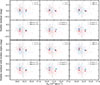 |
Fig. A.1. Same as Figure Fig. 2, but showing the full distribution of Hubble residuals without (top two rows) and with (bottom two rows) the broken-α standardisation of HV and NV SNe Ia. |
Secondly, in past studies, 99a-like and all 04gs-like SN Ia were probably included in normal SN Ia samples. Hence, in order to check the effect of removing these sub-types, we made the analysis by including 13 04gs-like SN Ia, where 9 would be NV and 4 would be HV and 34 99aa-like SN Ia, where 28 would be NV and 6 would HV, following same classification system as normals.
Lastly, we check the effect of selected phase threshold. In this work the peak sample is defined as within 5 days since maximum light, however, we also provide a more strict definition of the peak sample as within 3 days.
In Fig. A.2, we show the significances of the weighted average Hubble residual differences as a function of velocity (similar to Fig. 1), including all the selection effects considered. Regardless of the case there seems to be a none to weak relation, where the significance between the NV and HV SNe Ia seems to be mostly below 3σ level. Changing the velocity separation threshold from 12,000 km s−1 to 11,800 km s−1 slightly increasing the significances that include only normal SNe Ia. This effect seems to diminish once the 99aa-like and 04gs-like SNe are included in the samples. In general, inclusion of 99aa-like and 04gs-like SNe does not seem to be effecting anything significantly. We also clearly see that in all cases inclusion of template matched SNe to that sample increases the significances. Exclusion of those SNe would introduce a bias towards the high-mass galaxies since in most cases the SN without a redshift source is low-luminosity, hence a low-mass galaxy. That is why in all the analysis done in this work before and from this point includes all redshift sources. Lastly, using the broken-α standardisation from Ginolin et al. (2025b) increases the observed significances.
In Fig. A.3 and Fig. A.4, we explore the sample selection effect on the mass and colour steps, respectively (similar to Fig. 3). We notice hanging the velocity separation threshold from 12,000 km s−1 to 11,800 km s−1 seems to irrelevant in almost all cases, while using the broken-α standardisation seems to increase the significance slightly. Using 11,800 km s−1 also gives out a slightly higher significance difference between the mass steps of HV and NV SNe Ia (possibly due to increased sample size of HV SNe Ia), at 2.6σ, where 12,000 km s−1 separation were giving 2.2σ. Lastly, using a smaller phase yields lower significances in all analysis, however we observe that inclusion of 99aa-like and 04gs-like SNe have no effect to the observed significances.
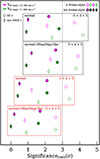 |
Fig. A.2. Significances of the weighted average Hubble residual differences as a function of velocity, following the same general analysis as Fig. 1. The circles represent samples that include all redshift sources, while the diamonds represent samples excluding template-matched redshift sources. Filled symbols indicate Hubble residuals standardised without the broken-α correction, and unfilled symbols show results with the broken-α correction. Magenta and green colours correspond to velocity splits at 12,000 km s−1 and 11,800 km s−1, respectively. The dashed vertical line marks the significance threshold. The black boxes show the results for samples in which the peak phase is within 5 days and the red boxes show the results in which the peak phase is within 3 days. The sub-types included in each analysis are noted within the boxes. |
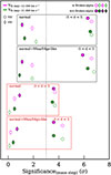 |
Fig. A.3. Significances of the weighted average Hubble residual differences as a function of mass following the same general analysis as Fig. 3. The circles represent the NV SNe Ia and the diamonds represent the HV SNe Ia. Filled symbols indicate Hubble residuals standardised without the broken-α correction, and unfilled symbols show results with the broken-α correction. Magenta and green colours correspond to velocity splits at 12,000 km s−1 and 11,800 km s−1, respectively. The dashed vertical line marks the significance threshold. The black boxes show the results for samples in which the peak phase is within 5 days and the red boxes show the results in which the peak phase is within 3 days. The sub-types included in each analysis are noted within the boxes. |
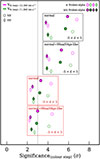 |
Fig. A.4. Significances of the weighted average Hubble residual differences as a function of global colour (g − z), following the same general analysis as Fig. 3. The circles represent the NV SNe Ia and the diamonds represent the HV SNe Ia. Filled symbols indicate Hubble residuals standardised without the broken-α correction, and unfilled symbols show results with the broken-α correction. Magenta and green colours correspond to velocity splits at 12,000 km s−1 and 11,800 km s−1, respectively. The dashed vertical line marks the significance threshold. The black boxes show the results for samples in which the peak phase is within 5 days and the red boxes show the results in which the peak phase is within 3 days. The sub-types included in each analysis are noted within the boxes. |
All Tables
Weighted averages and significances of the Hubble residuals for the HV and NV samples for different parameters.
All Figures
|
Fig. 1. Hubble residuals as a function of Si IIλ6355 velocity (vSi). Top Left: Hubble residuals for NV (black points) and HV (red points) including all redshift sources (see: Section 2.1 for the redshift sources). Top Middle: Same as on the left, but without the template-matched redshift sources. Top right: Same as on the left, but with the template-matched redshift sources alone. Bottom left: Hubble residuals with broken alpha from Ginolin et al. (2025b) for all redshift sources included in the sample. Bottom middle: Same as on the bottom left, but without the template-matched redshift sources. Bottom right: Same as on the bottom left, but with the template-matched redshift sources alone. In all panels, the horizontal black and red lines represent the weighted mean of the Hubble residuals in the NV and HV bins, respectively, where the shaded regions shows the 1σ uncertainty of the weighted means. The vertical dashed grey line represents the criterion (vSi = 12, 000 km s−1) that we used to separate the HV and NV SN Ia samples. The difference of the weighted averages of the HV and NV samples, along with the significances, are shown in each panel. |
| In the text | |
|
Fig. 2. Hubble residuals without (top two rows) and with (bottom two rows) the broken-α standardisation of HV and NV SNe Ia are shown as a function of Si IIλ6355 velocity (all redshift sources included), separated by low and high values of x1, c, dDLR, host galaxy mass, global colour, and local colour. In each plot, the weighted averages (corresponding to high and low values of the parameter) for HV and NV SNe Ia are shown as stars. The vertical dashed line represents the criterion (vSi = 12, 000 km s−1) we used to separate the HV and NV SN Ia samples. To highlight the relative offsets, the panels show a zoomed-in view of the Hubble residuals. The full-scale version is provided in Appendix A. |
| In the text | |
|
Fig. 3. Hubble residuals as a function of global and local host galaxy mass (top two rows). The top row of plots displays the Hubble residuals without the broken-α standardisation, and the bottom row shows the Hubble residuals with it. In each plot, black circles represent NV SNe Ia, and red circles represent HV SNe Ia. The horizontal black and red lines show the weighted averages of the Hubble residuals for the NV and HV samples, respectively, and the shaded regions represent the 1σ uncertainties of these averages. The vertical dashed lines at log(M★/M⊙) = 10 show the division between low- and high-mass samples based on global host galaxy mass in the left panels, and the dashed lines at log(M★/M⊙) = 8.9 show the division based on local host galaxy mass in the right panels. The difference in the weighted averages between the low- and high-mass samples, along with the corresponding significances, are shown in each panel. The Hubble residuals as a function of global and local g–z colours are shown in the bottom two rows. The vertical dashed line represents the criterion (g–z = 1) we used to separate the low- and high-colour environments. |
| In the text | |
|
Fig. 4. Hubble residual plots without and with the broken alpha standardisation as a function of host galaxy mass for HV and NV SNe Ia split by dDLR. The black and red dots represent the NV and HV SNe Ia, respectively. The vertical dashed line represents the criterion (log(M★/M⊙) = 10 for the global mass samples). In each plot, the horizontal dashed lines represent the weighted mean of the Hubble residuals, and the shaded regions shows the 1σ uncertainty of the weighted means. The difference of the weighted averages between the low- and high-mass samples along with the significances are shown in the label. |
| In the text | |
|
Fig. 5. Same as Fig. 4, but as a function of global colour (g–z) for HV and NV SNe Ia split by dDLR. The vertical dashed line represents the criterion (g–z = 1) we used to separate the global low- and high-colour samples. |
| In the text | |
|
Fig. 6. Distribution of NV and HV SNe Ia across host galaxy mass and global colour. HV and NV SNe Ia are represented with red and black circles, respectively. The vertical dashed line at log(M★/M⊙) = 10 marks the division between low- and high-mass galaxies, and the horizontal dotted line at g–z = 1 marks the division between blue and red hosts. |
| In the text | |
|
Fig. A.1. Same as Figure Fig. 2, but showing the full distribution of Hubble residuals without (top two rows) and with (bottom two rows) the broken-α standardisation of HV and NV SNe Ia. |
| In the text | |
|
Fig. A.2. Significances of the weighted average Hubble residual differences as a function of velocity, following the same general analysis as Fig. 1. The circles represent samples that include all redshift sources, while the diamonds represent samples excluding template-matched redshift sources. Filled symbols indicate Hubble residuals standardised without the broken-α correction, and unfilled symbols show results with the broken-α correction. Magenta and green colours correspond to velocity splits at 12,000 km s−1 and 11,800 km s−1, respectively. The dashed vertical line marks the significance threshold. The black boxes show the results for samples in which the peak phase is within 5 days and the red boxes show the results in which the peak phase is within 3 days. The sub-types included in each analysis are noted within the boxes. |
| In the text | |
|
Fig. A.3. Significances of the weighted average Hubble residual differences as a function of mass following the same general analysis as Fig. 3. The circles represent the NV SNe Ia and the diamonds represent the HV SNe Ia. Filled symbols indicate Hubble residuals standardised without the broken-α correction, and unfilled symbols show results with the broken-α correction. Magenta and green colours correspond to velocity splits at 12,000 km s−1 and 11,800 km s−1, respectively. The dashed vertical line marks the significance threshold. The black boxes show the results for samples in which the peak phase is within 5 days and the red boxes show the results in which the peak phase is within 3 days. The sub-types included in each analysis are noted within the boxes. |
| In the text | |
|
Fig. A.4. Significances of the weighted average Hubble residual differences as a function of global colour (g − z), following the same general analysis as Fig. 3. The circles represent the NV SNe Ia and the diamonds represent the HV SNe Ia. Filled symbols indicate Hubble residuals standardised without the broken-α correction, and unfilled symbols show results with the broken-α correction. Magenta and green colours correspond to velocity splits at 12,000 km s−1 and 11,800 km s−1, respectively. The dashed vertical line marks the significance threshold. The black boxes show the results for samples in which the peak phase is within 5 days and the red boxes show the results in which the peak phase is within 3 days. The sub-types included in each analysis are noted within the boxes. |
| In the text | |
Current usage metrics show cumulative count of Article Views (full-text article views including HTML views, PDF and ePub downloads, according to the available data) and Abstracts Views on Vision4Press platform.
Data correspond to usage on the plateform after 2015. The current usage metrics is available 48-96 hours after online publication and is updated daily on week days.
Initial download of the metrics may take a while.