| Issue |
A&A
Volume 705, January 2026
|
|
|---|---|---|
| Article Number | A35 | |
| Number of page(s) | 16 | |
| Section | The Sun and the Heliosphere | |
| DOI | https://doi.org/10.1051/0004-6361/202556465 | |
| Published online | 07 January 2026 | |
Insights into penumbral formation from high-resolution photospheric and chromospheric observations
1
Astronomical Institute of the University of Bern, Sidlerstrasse 5, 3012 Bern, Switzerland
2
Institute for Solar Physics, Dept. of Astronomy, Stockholm University, AlbaNova University Centre, 106 91 Stockholm, Sweden
3
Institute of Theoretical Astrophysics, University of Oslo, PO Box 1029 Blindern, N-0315 Oslo, Norway
4
Rosseland Centre for Solar Physics, University of Oslo, PO Box 1029 Blindern, N-0315 Oslo, Norway
★ Corresponding author: This email address is being protected from spambots. You need JavaScript enabled to view it.
Received:
17
July
2025
Accepted:
31
October
2025
Abstract
Context. Penumbra formation occurs within hours and remains not fully understood. Two competing theories suggest either a top-down mechanism, whereby the chromospheric magnetic field becomes more horizontal, or a bottom-up process involving flux emergence near the sunspot umbra.
Aims. We investigate penumbra formation and test both hypotheses by inferring and analyzing the full magnetic field from the photosphere to the chromosphere above a forming sunspot.
Methods. We applied Milne-Eddington, weak field approximation, and the multiatom non-local thermodynamic equilibrium inversion code STiC to obtain the model atmosphere that reproduces the Stokes profiles of Fe I 6302 Å and Ca II 8542 Å observed at the Swedish Solar Telescope, complementing the analysis with images taken in Hβ.
Results. A penumbra formed only in the southern sector of a sunspot in AR 13010 on May 15, 2022. We find that a preexisting, strong (> 500 G) and nearly horizontal magnetic field in the chromosphere is a key prerequisite. Penumbral filaments grew southward where localized flux emergence was observed, accompanied by strong redshifts (2–3 km s−1) throughout the atmospheric layers. These redshifts likely represent field-aligned horizontal flows, possibly combining the onset of the Evershed flow and a siphon-like flow driven by field-aligned pressure gradients.
Conclusions. Our findings indicate that penumbra formation results from both top-down and bottom-up processes. While strong horizontal chromospheric magnetic fields are a necessary boundary condition, flux emergence initiates filament growth. The fallen flux tube model is ruled out, based on clear bottom-up signatures, though it remains unclear why the chromospheric and photospheric fields become more horizontal concurrently. Extended spectropolarimetric data are needed to get a deeper insight.
Key words: Sun: chromosphere / Sun: magnetic fields / Sun: photosphere / sunspots
© The Authors 2026
 Open Access article, published by EDP Sciences, under the terms of the Creative Commons Attribution License (https://creativecommons.org/licenses/by/4.0), which permits unrestricted use, distribution, and reproduction in any medium, provided the original work is properly cited.
This article is published in open access under the Subscribe to Open model. This email address is being protected from spambots. You need JavaScript enabled to view it. to support open access publication.
1. Introduction
Sunspots form when twisted magnetic field lines emerge from below the solar surface and become visible as scattered dark spots, called pores. The convective motion and further emerging flux let the pores grow and coalesce, creating a more concentrated “spot” of magnetic flux (Zwaan 1985; Schlichenmaier et al. 2010b). The concentrated magnetic flux suppresses convection, which allows the plasma in the spot to cool more than the surrounding granulation, making the spot appear dark compared to the rest of the Sun. A spot of concentrated magnetic flux is only considered a sunspot when it starts to form a penumbra.
One identifying property of the penumbra is the formation of a radial outflow, called the Evershed flow (Evershed 1909), which follows the magnetic field in the penumbra (Bellot Rubio et al. 2003). The average inclination of the magnetic field of a penumbra in the photosphere increases from approximately 40° at the umbra–penumbra boundary to about 70° at the outer edge of the penumbra. Despite our understanding of the formation of the umbra part of the sunspot (dark central region), the formation of the penumbra is still elusive. In particular, the question of when and how penumbra formation starts is still debated. Specialized 3D magnetohydrodynamic simulations are unable to produce a penumbra without introducing an additional top boundary condition, making the magnetic field above the sunspot more inclined (Rempel et al. 2009; Rempel 2011, 2012). Rempel (2011) discussed how the boundary conditions of the simulation generally produce a less inclined magnetic field above the sunspot than expected.
A similar behavior was found in Rempel et al. (2009), in which a pair of sunspots with opposite polarity was simulated. The penumbra only formed in the direction of the opposite polarity, which had an automatically larger inclination compared to the other directions. This has independently been observed in observations by Rezaei et al. (2012), where they found that only under high magnetic field inclination ( ≥ 60° ) did penumbra formation start, and no associated flux emergence was observed.
Flux emergence near the umbra is another proposed mechanism for the start of penumbra formation (e.g., Lites et al. 1998; Leka & Skumanich 1998; Louis et al. 2013; Lim et al. 2013; Li et al. 2018). This theory is supported by observations of emerging flux that is co-spatial and co-aligned with developing penumbral filaments. However, other studies have found that the earliest forming penumbral sectors are not associated with locations of significant flux emergence (Rezaei et al. 2012; Murabito et al. 2018; Schlichenmaier et al. 2010a,b). Lindner et al. (2023) observed a partially formed penumbra in NOAA AR 12776. Magnetogram data showed a correlation between the penumbra size and the magnetic flux. They observed an average magnetic field inclination of 68° in the chromosphere on the side where the penumbra formed. No difference was found between the magnetic field inclination in the photosphere on the side where a penumbra formed, compared to the no-penumbra side. They concluded that a high magnetic field inclination in the chromosphere is a necessary boundary condition to initiate penumbra formation and that emerging magnetic flux drives the formation. Studies of the chromospheric magnetic field leading to the onset of penumbra formation are rare (e.g., Murabito et al. 2016; Lindner et al. 2023).
Several studies have reported observations of a penumbra-like structure in the chromosphere hours before a penumbra becomes visible in the photosphere (Shimizu et al. 2012; Romano et al. 2013, 2014; Murabito et al. 2016). Unfortunately, none of these studies included chromospheric polarimetric measurements, and the magnetic field in these structures could not be quantitatively analyzed. None of these studies observed flux emergence to be associated with the formation of the penumbra. It has also been observed that rapid changes in the magnetic field, for instance through solar flares (Wang et al. 2004) or gradual changes through fragmentation by light bridges, can make the penumbra disappear in the disrupted area (Romano et al. 2020). After the original magnetic field configuration was restored, the penumbra reformed. To this day, it is an open question whether penumbra formation is a top-down process, a bottom-up process, or a combination of the two. In this work, we analyze the formation of a penumbra on the southern side of a collection of pores to investigate whether the top-down or the flux-emergence model is more likely for penumbra formation.
2. Observations and data preparation
We collected spectro-polarimetric observations of Fe I 6302 Å and Ca II 8542 Å with the CRISP instrument, and complementary data with CHROMIS in Ca II K and Hβ at the Swedish 1-m Solar Telescope (SST) on La Palma, Spain (Scharmer et al. 2003; Scharmer 2006; Scharmer et al. 2025).
The observations were taken on May 16, 2022. Forty scans were recorded from 08:28-08:49 UTC and twelve scans from 12:16-12:23 UTC, all at a cadence of 28.3 s. We selected 31 scans with good seeing conditions for analysis from the first observation and 2 scans from the second observation. The collection of pores was observed in NOAA AR13010, located at −32.0° east and −14.56° south at 08:28 UT, with a heliocentric angle of μ = 0.826. The evolution of AR13010 around the observation times with SST is presented in Fig. 1, using observations from the Helioseismic Magnetic Imager (HMI, Scherrer et al. 2012) on board the Solar Dynamics Observatory (SDO, Pesnell et al. 2012). The white square shows the field of view (FOV) of CRISP. We observed the same AR on May 15 and 17 also, but were unable to use these data due to poor seeing and because the FOV did not cover the southern part of the spot where the penumbra formed first. Figure 2 shows the evolution of the sunspot observed with HMI on May 16, comparing the continuum image and the inverted and Lambert Cylindrical Equal-Area (CEA) transformed magnetic field (series: hmi.sharp_cea_720s). The vertical magnetic field (henceforth HMI magnetogram) reveals where flux emergence might have triggered penumbra formation. However, at the resolution of HMI, we did not detect any flux emergence in the close vicinity of where the penumbra formed. This becomes more important later when we analyze our high-resolution observations recorded with SST. The spectral range and sampling configuration for all the spectral lines we observed are listed in the Table 1. The Fe I 6302 Å was recorded with 13 wavelength points. The two outermost wavelength points were recorded with a separation of 0.08 Å. The other points are equispaced according to Table 1. The Ca II 8542 Å line was recorded at 16 non-equidistant wavelength points. The wavelength spacing followed a symmetrical grid around the line core. In the blue wing, the outermost wavelength point was recorded with a difference of Δλ = 0.4 Å to the next point. Two subsequent wavelength points were recorded with Δλ = 0.2 Å and all others until the line core with Δλ = 0.1 Å. The outermost point in the red wing had a spacing of Δλ = 0.8 Å to sample lower solar layers. The observations were reduced with SSTRED (de la Cruz Rodríguez et al. 2015; Löfdahl et al. 2021), which uses a multiobject multiframe blind deconvolution image restoration technique (Löfdahl 2002; Van Noort et al. 2005). Figure 3 shows the intensity images from the first and last observation, respectively. The southern sector has a much clearer canopy structure, forming a super-penumbra, while the canopy appears more chaotic and twisted in the northern part.
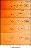 |
Fig. 1. Overview of the evolution of NOAA active region AR13010 from May 15 – 17 with HMI. In the bottom left of each image is the timestamp of the HMI observation. The white square indicates the full FOV of CRISP. The black boxes on the right indicate the times at which we took SST observations. |
Parameters for each spectral line window.
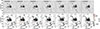 |
Fig. 2. Detailed evolution of the sunspot. The upper panel displays the continuum intensity image for reference, and the lower panel shows the vertical magnetic field in the local reference frame. To cover the most important times of the penumbra formation, we display one HMI frame each hour between 08:00 and 12:00, and additionally one frame at 05:00, roughly three hours before the SST observations, and one frame at 14:00, roughly two hours after our last observation. The small black box indicates FOV selection, which we inverted with STiC. |
3. Methods
3.1. Inversion of Fe I 6302 Å using the Milne-Eddington approximation
To calculate the magnetic field in the photosphere from Fe I 6302 Å, we used the Milne Eddington (ME) inversion code PyMilne1 (de la Cruz Rodríguez 2019). The ME model assumes a linear source function and height-independent values for each magnetic field component and the line-of-sight (LOS) velocity. While PyMilne includes options for spatial and temporal regularization (de la Cruz Rodríguez & Leenaarts 2024), we did not apply them in this study. The Fe I 6302 Å line generally forms in local thermodynamic equilibrium (LTE), and can be approximated by the ME model. For instance, the MERLIN code, developed for the Hinode/SOT Spectro-Polarimeter, employs an ME approach to invert the Fe I 6301 Å and 6302 Å line pair (e.g., Lites et al. 2013). The Milne-Eddington model provides a good first approximation for both the photospheric magnetic field and the LOS velocity.
3.2. Determination of the chromospheric magnetic field using a spatially regularized weak field approximation
The Ca II 8542 Å line’s formation is complex, with its wings originating in the photosphere and its core in the chromosphere. Its atmospheric parameters and source function vary significantly with height, violating the fundamental assumptions of the ME model. We therefore used the weak field approximation (WFA) to obtain an initial estimate of the chromospheric magnetic field (Landi Degl’Innocenti & Landi Degl’Innocenti 1973; Jefferies et al. 1989). More details are given in Appendix B.
3.3. Inversion with STiC of selected field of view
The results of the ME and WFA gave us a general picture of the forming sunspot and guided our selection of a smaller FOV to jointly invert the Fe I 6302 Å and Ca II 8542 Å lines with STiC. We obtained a 3D depth-stratified model of the solar atmosphere. Each pixel is modeled as a 1D plane-parallel atmosphere along the line of sight (LOS). STiC utilizes the spectral synthesis code RH (Uitenbroek 2001), which can simultaneously solve for the atomic population levels of several atomic species, including partial redistribution effects. The RH version included in STiC has been modified to include the contribution of non-LTE hydrogen ionization in the calculation of the electron density (see the appendix of Leenaarts et al. 2007). The depth stratification of pressure and density is computed under the assumption of hydrostatic equilibrium. The physical parameters of the model are returned as a function of the optical depth scale at 5000 Å (log τc). For each physical parameter, a number of nodes are placed at specific depths, which are then iteratively adjusted by STiC to match the synthetic spectral shapes with the observed spectral shapes. Between node locations, the model is interpolated to a common log τc grid for all physical parameters. Since we did not invert the Ca II K line, we could run STiC in complete redistribution mode, which substantially reduced computation time (Uitenbroek 1989; Sukhorukov & Leenaarts 2017).
For the inversion, we interpolated the observations to an equally spaced wavelength grid and normalized to the quiet Sun continuum brightness, given by the FTS solar atlas, accounting for the center to solar limb variation (Allen 1973). The intensity calibration was refined as a post-processing step to ensure full consistency between both lines before the inversion. We recalibrated the Fe I 6302 Å directly by fitting an average profile of a quiet Sun patch in the observation to the FTS atlas. The data preparation was performed using additional Python methods provided together with STiC, and adjusted by the authors to the present use case. The initial model for STiC was prepared on an equally spaced log τc grid from 2.0 to −6.8, with a spacing of 0.12. For the initial physical parameters, we used a rough quiet Sun temperature profile, and used the results from the ME and WFA as bottom and top boundary conditions for the magnetic field, and interpolated in between.
For the LOS velocity (vlos), we used the ME vlos map, and for the microturbulence, we used a constant value of 1 km s−1. We inverted the data, performing three cycles, where the first cycle was run with a maximum of five iterations, only changing the thermodynamic model parameters, and in the other two cycles, a maximum of three iterations, changing all parameters to fit the observation. We noticed that using more iterations quickly runs into overfitting, and that only a few nodes were necessary to capture the physics of the atmosphere. The optimal node configurations were determined through a systematic parameter search, and after successfully inverting the observation from 12:16 UT, we inverted the rest of the observations using the same procedure.
The final node configurations used per cycle are listed in Table 2. In the last cycle, we set the middle node for all parameters except temperature and azimuth at log τc = −2.5, to capture the transition point between the regimes the Fe I 6302 Å and the Ca II 8542 Å are sensitive to. The final inversion results were verified through computation of the goodness of fit χ2 criterion with which the inversion of STiC is driven (de la Cruz Rodríguez et al. 2019), and through the identification of well-known physical features in sunspots and penumbra. For instance, in videos of the LOS velocity in the chromosphere, we could observe penumbral waves, the temperature maps follow the intensity maps of the continuum and the chromospheric temperature maps have the same structures as found in the intensity maps of the core wavelengths of, for instance, Ca II 8542 Å.
Node configurations for inversion with STiC.
To reduce computation time, we only inverted every second pixel in the first cycle. STiC did not converge to a solution in all pixels in the first cycle. For the further cycles, we therefore interpolated the solutions between pixels that successfully converged. To determine which pixels converged, we computed the goodness of fit χ2 for each pixel as follows. First, we standardized the spectral profiles using the average observed profile and the standard deviation at each wavelength, to obtain the signal-to-noise ratio (S/N) at each wavelength. Then we computed the sum of the squared distances between the synthetic and observed profiles, divided by the number of wavelength positions to compute the reduced χ2 goodness of fit for each Stokes component. To determine which profiles were badly inverted by STiC we used the following minimum criteria for χ2: For Fe I 6302 Å Stokes Iχ2 > 1.1, Stokes Q & Uχ2 > 3.6, and Stokes Vχ2 > 2.3. The criteria were systematically chosen by comparing the pixels flagged in result maps of different thresholds. We selected the thresholds that best matched incoherencies in the result maps. Pixels with a Q, U, V < 5 ⋅ 10−3 were ignored to omit flagging inverted pixels with no or very low polarization (< 0.5%). For comparison, the noise level for CRISP polarization detection is ∼2 ⋅ 10−3 (Ortiz et al. 2010); thus, we chose a conservative threshold.
With the pixels that reached any of the minimum χ2 thresholds, we trained a k-nearest neighbor (KNN) regressor from the Python library scikit-learn2 (Pedregosa et al. 2011) and inferred all the “failed” and skipped pixels through inference. The Stokes components were combined into a single vector, and the KNN was trained to infer one physical parameter at a time (for instance, temperature). The KNN regressor has a natural smoothing effect on the data, as using, for instance, k = 5 to train the regressor results in the solution being the average of the five closest pixels with respect to spectral shape. We observed that the five closest neighbors to the pixel in question always coincided with the spatially closest pixels. Therefore, the KNN regressor naturally takes the domain around the inferred pixel into account, making it a strong tool to also estimate the physical parameters well for pixels with a low S/N. For low-S/N patches, the solution found with STiC remained very close to the KNN-inferred solution. We additionally smoothed maps with a Gaussian kernel smoother wherever we observed such a behavior.
3.4. Formation heights of Fe I 6302 Å and Ca II 8542 Å
We verified the formation heights of both spectral lines by computing the response functions for the magnetic field components, temperature, and LOS velocity with STiC. Response functions are defined as the partial derivative of the computed Stokes parameter by any physical parameter of interest, and are a function of wavelength and height or optical depth (del Toro Iniesta & Ruiz Cobo 2016). The core of the Fe I 6302 Å line forms between log τc = 0 and log τc = −2, covering the photosphere down to the visible surface of the Sun. The core of the Ca II 8542 Å line forms between log τc = −4 and log τc = −5, well in the chromosphere, and the wings down to log τc = −2. From this, we infer that our results from the ME inversions are representative of the photosphere at around log τc = −1 (in agreement with previous studies by Orozco Suárez et al. 2010; Borrero et al. 2014), and the WFA results for the chromosphere at around log τc = −4.
3.5. Disambiguation and transformation to the local reference frame
The magnetic field vector was transformed from the instrument’s LOS reference frame to a local reference frame (LRF) on the solar surface following the method of Gary & Hagyard (1990). To disambiguate the azimuth map in the STiC FOV, we used a potential field extrapolation from Wheatland et al. (2000) applied to the LOS magnetic field and extended the azimuth map to [0° ,360° ]. We flipped the azimuth direction by 180° at each position where the difference to the potential field extrapolation exceeded 90°. The methods for the potential field extrapolation were extracted and adjusted from the ISPy library3 (Díaz Baso et al. 2021). Since we implemented the LRF transformation ourselves, we tested it with a test vector field. The LOS velocities cannot be transformed to the LRF; however, we corrected them, such that the average velocity in the quiet Sun is almost zero.
4. Results
4.1. Photospheric magnetic field and LOS velocity with Milne Eddington
The results of the ME inversion for the photospheric Fe I 6302 Å line are shown in Fig. 4. From left to right, we show the LOS magnetic field B||, inclination θ, azimuth ϕB, and LOS velocity vLOS, at two different times. The top panel was observed at 08:28 UT, and the bottom panel at 12:21 UT, around four hours apart. The contours of the umbra and penumbra boundaries were drawn by marking the area greater than a specific intensity value in the Ca II 8542 Å wing. In the upper panel, a partial penumbra is already present in the left southern sector of the spot. In the lower panel, this part of the penumbra has diminished, while in the rest of the southern sector, a penumbra has formed. The magnetic field inclination is much larger (∼150°) in the northern sector, indicating almost vertical magnetic field lines, compared to the southern sector (∼90° −120°). In the southern sector where the penumbra forms, the LOS inclination ranges from 75° to 125°, indicating a magnetic field that is oriented more perpendicularly to the LOS. The LOS velocity maps show the presence of most likely the onset of an Evershed outflow, where the penumbra formed. Since the observation is located at ∼ − 32° E and ∼ − 14.5° S, the Evershed flow should be redshifted in the southern sector of the penumbra, which matches the vLOS map. The strong redshift at ∼2 km s−1 follows the contour of the penumbra filaments. Except for the magnetic field inclination, we did not notice any substantial differences between the northern and southern sectors of the forming sunspot. We did not disambiguate the azimuth map or transform the ME results to the LRF. This will be performed for the more sophisticated STiC inversions, together with an analysis of the flux emergence in Sect. 4.3.
4.2. Chromospheric magnetic field obtained with the weak field approximation
In this section, we analyze the chromospheric magnetic field with the WFA applied to the Ca II 8542 Å line and compare it with the values derived by inversions in Sect. 4.3. Figure 5 shows the LOS (B||) and perpendicular (B⊥) components of the chromospheric magnetic field at the same two timestamps presented in Fig. 4. Immediately apparent is that the chromospheric magnetic field is much smoother than in the photosphere, and the perpendicular magnetic field does not change much over the time the penumbral filaments grow.
At 12:21 UT, the perpendicular magnetic field became weaker around the left part of the penumbral filaments, which were already present during the first observation. The main difference between the northern and southern sectors is the difference in the perpendicular magnetic field strength. In the northern sector of the sunspot, the Stokes Q and U signals are very weak, resulting in a low measured B⊥ and indicating the absence of a significant, coherent transverse field. This lack of a strong horizontal magnetic canopy may be a key reason why a penumbra never formed there. In the southern sector, clear magnetic field structures at 600–1000 G are visible, extending even further than the red contour, which indicates the extent of the forming penumbra. Comparing the two observations, we note that the overall structure of this canopy remains largely unchanged over the four-hour period. However, in the later observation at 12:21 UT, the perpendicular magnetic field has weakened in the western part of the southern sector. This location corresponds to the area where the initial penumbral segment, seen at 08:28 UT, later diminished in the photosphere.
4.3. Full non-LTE depth stratified results for the physics of the photosphere and chromosphere
The results from the inversions with STiC give us a 3D picture of the solar atmosphere and allow us to investigate better how the photosphere and the chromosphere are connected. Sections 4.1 and 4.2 show that a strong horizontal canopy magnetic field in the chromosphere seems to make the difference between where a penumbra formed and where it did not. Because we are unable to invert the entire observation due to computational limitations, we limited our STiC inversions to the representative area marked with a block box in Fig. 3. Since the observation was taken at an angle θ ∼ 34.3° and μ = 0.826 to the disc center, opposite polarities appearing in the forming penumbra patch can come from projection effects, when the magnetic field horizontally follows the solar surface. Therefore, we transformed all our results for the magnetic field with STiC to a LRF. To avoid ambiguity, we will use the following standard terminology throughout this section: Bz refers to the vertical component of the magnetic field (perpendicular to the solar surface). Bh refers to the horizontal component of the magnetic field (parallel to the solar surface), calculated as  . These LRF components are distinct from the LOS components (B|| and B⊥) discussed in previous sections.
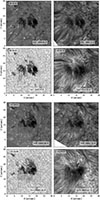 |
Fig. 3. Overview image of the observation at 08:28 (upper set of panels) and 12:19 (lower set of panels). In each set of panels, the upper left panel shows the Hβ far wing image, the upper right panel the Hβ core forming in the chromosphere, the lower left panel shows the continuum image in Fe I 6302 Å and the lower right the line core of Ca II 8542 Å, also forming in the chromosphere. The black box indicates where we selected a subframe to invert the data with STiC. |
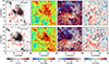 |
Fig. 4. Milne-Eddington result maps showing the LOS magnetic field strength, B||, inclination, θ, azimuth, ϕB, and LOS velocity, vLOS, for the observation taken at 08:28 UT (upper panel) and 12:21 UT (bottom panel) for the 6302 Å line. The black contours indicate the extent of the umbra in the forming sunspot, while the red contours show the extent of the penumbra, which has formed by 12:21 UT in the southern sector. |
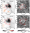 |
Fig. 5. Chromospheric magnetic field inferred from the Ca II 8542 Å under the WFA. The panels show the LOS magnetic field strength (left) and the perpendicular magnetic field strength (right). The contours are identical to Fig. 4. |
In the center part of the FOV inverted with STiC, we noticed substantial flux emergence, which was still present at 12:21 UT, as can be seen in the upper panel of Fig. 6. The transformation to the LRF shows that most of the positive vertical magnetic field vanishes; thus, the large distribution of positive magnetic field flux in the upper panel primarily stems from projection effects. This is further supported by the fact that we did not observe any strong vertical magnetic field in the penumbra, in contrast to the umbra in the HMI observations (see Fig. 2).
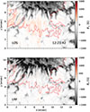 |
Fig. 6. Comparison between the vertical magnetic field in the LOS frame (upper panel) and the local reference frame (lower panel). The red and black contours indicate the size of the penumbra and umbra, respectively. The positive magnetic flux is only visible in the LOS frame, which may indicate projection effects. |
The full results obtained with STiC for log τc = 0.0 and log τc = −4.4 as representative heights of the photosphere and the chromosphere, respectively, are presented in the appendix (Fig. A.1 and Fig. A.2), and the most relevant parameters are shown in Fig. 7. To show the evolution of the features, we selected six representative timestamps, which are used in all the following figures that show temporal evolutions. In the left part of the forming penumbra presented in Fig. A.1, in rows 1–5, the magnetic field inclination is roughly horizontal to the solar surface and increases to ∼150° closer to the spot, indicating that the magnetic field lines dip down and into the umbra. In this part, strong redshifts in vLOS show the established Evershed flow in the partially formed penumbral filaments. In row 6, the inclination is mixed with streaks of highly inclined magnetic field, and the vLOS redshifts appear weaker. This agrees well with the lower horizontal magnetic field strength found in Fig. 5 in the same area. In the center of the FOV, a structure of negative magnetic field (up to −1000 G) is present. Following the part within the vertical dashed lines, the negative magnetic field streak moved southward and disappeared by 12:21 UT. Based on HMI magnetograms, it was already present before our SST observations and originated as expelled magnetic flux from the main pore, which later formed the penumbra. From 0″ to 1 5 in the same Fig. A.1, there is a small pore with a positive magnetic field, which appears around 06:48 UT and is present until 11:48 UT in the HMI magnetograms. Both the negative magnetic field streak and the pore with the positive magnetic field are pushed outside of the inverted STiC-FOV with the growth of the penumbra and strongly resemble moving magnetic features (MMFs Harvey & Harvey 1973; Sainz Dalda et al. 2012). Other pores with positive polarity also appear north of the spot and disappear again, but no stable penumbra forms. The magnetic field inclination along the vertical dashed lines in Fig. A.1 shows a growing area of close-to-horizontal magnetic field in rows 1 to 5, with high inclination closer to the umbra and low inclination further away from the umbra. Co-spatial with the changing magnetic field configuration, penumbral filaments start forming. In row 6, the magnetic field inclination is horizontal in a wide area around the vertical dashed lines, and redshifts in the vLOS maps in that area indicate an established Evershed flow. The evolution of the magnetic and velocity structure within the vertical dashed lines in Fig. A.1 will be analyzed in Sect. 4.4.
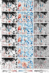 |
Fig. 7. STiC inversion result maps (vertical magnetic field, Bz, LOS velocity, vLOS, and Fe I wing intensity) of the region of interest marked in Fig. 3. Dark red contours indicate where the vertical magnetic field exceeds 20 G, to better follow the evolution of the positive magnetic flux patch. Arrows are drawn to indicate the flow pattern of the emerging flux. Gray and black contours indicate the size of the penumbra and umbra, respectively. Within the area marked by the vertical dashed lines, the vertical structure of the atmosphere is analyzed in more detail. |
Figure 7 provides a detailed view of the small-scale magnetic activity, co-spatial and co-temporal with the forming penumbral filaments. Along the vertical dashed lines, a small patch of positive magnetic field at y = 5″ becomes visible. Its extent is marked through dark red contours in Fig. 7, which indicate where the vertical magnetic field exceeds 20 G (Bz > 20 G). Row 1 shows that at the location of the arrows, two small positive magnetic field patches are streaming southward, roughly moving in the direction indicated by the arrows. In row 2, a more positive magnetic field becomes visible and coalesces to one single patch (row 3). The positive magnetic field patch streams southward with an average velocity of ≈0.12 − 0.15″ per minute, which corresponds to ≈1.4 − 1.8 km s−1. The growing penumbra follows the position of the positive magnetic field patch until about 08:40 (row 4). During the time between rows 4 and 5, the forming penumbra filament is disturbed by a convective cell rising and pushing in between the positive magnetic flux patch and the lower end of the penumbral filaments. Three hours later, in the same position as well as left and right of it, a full penumbra has formed, as is visible in row 6 of the intensity plot (rightmost column).
Co-spatially with the positive magnetic field patch, we observed strong redshifts in the LOS velocity, reaching and even exceeding 2 km s−1. We tracked the position of the maximum velocity within the patch, and in Fig. 8 we present the LOS velocity and magnetic field in time. The velocity gradually increases with the formation of the positive magnetic flux patch, and then starts decreasing rapidly around scan number 20 (taken at 08:44 UT). The vertical magnetic field strength also gradually increases until scan number 14 (08:40 UT), and then gradually decreases again until scan number 20. After scan number 20, both values only slightly increase again, but we did not see any further influence on the formation of the penumbra until 08:49 UT, the end of the first observation recording. In Fig. 8, only the last two scans are from the observation starting at 12:16 UT, where the penumbra had already formed. The presence of strong, persistent redshifts in the vLOS maps is a key finding. They reach over 2 km s−1, and are precisely co-spatial with the emerging positive polarity (Bz > 0) patch. The co-location of an emerging magnetic feature with strong redshifts, rather than the expected blueshifts, will be addressed in the discussion.
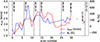 |
Fig. 8. Temporal evolution of the vertical velocity (red) and vertical magnetic field strength (blue) at the location of maximum velocity as seen in the velocity maps of Fig. 6. The vertical dashed lines indicate the timestamps for which we present the results. |
4.4. Vertical structure of the solar atmosphere along the patch of emerging flux
To investigate the connection between the photosphere and the chromosphere, we made vertical cuts along the vertical dashed lines in Figures A.1, A.2, and 7. The vertical structure of the magnetic field component Bz, and the magnetic field inclination θ are presented in Fig. 9, and the LOS velocity vLOS and horizontal magnetic field strength Bh are presented in Fig. 10.
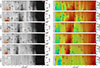 |
Fig. 9. Structure of the vertical magnetic field strength (left) and inclination (right) with height. The arrows indicate the direction of the magnetic field. The black contours in the left panel indicate the vertical magnetic field strength, while in the right panel, they display magnetic field inclination. The arrows indicate the direction of the magnetic field. In panels two to four, the emerging flux is visible as a positive patch of magnetic flux. |
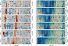 |
Fig. 10. Same as Fig. 9, but for the LOS velocity vLOS, and the horizontal magnetic field strength, Bh. In the left panel, the black contours show the vertical magnetic field strength, Bz, which is also depicted in the left panel of Fig. 9. The black contours in the right panel indicate the horizontal magnetic field strength, while the red contours indicate the vertical magnetic field strength. |
In some vertical columns (e.g., around the 7″ mark in the top panel of Fig. 9), the arrows suddenly point away from the sunspot. In these pixels STiC converged to an erroneous solution, which can also be seen in the azimuth maps of Figures A.1, and A.2. Through the change to the LRF, the azimuth, inclination, and magnetic field strength influence each other, which leads to the propagation of errors in the azimuth to the other magnetic field components. We therefore exclude these isolated columns from our physical interpretation.
In row 1 of the left column of Fig. 9, the positive magnetic field patch is not yet visible. Rows 2 to 4 show how the positive magnetic field patch’s strength increases to > 100 G, but does not noticeably affect the chromosphere. In row 5, the positive flux decreases. The magnetic field gradually becomes more horizontal throughout the atmosphere between x = 4.5″ and 6″ in panels 1 to 4. The position coincides with the location of the emerging positive flux and exceeds its height, which is also reflected in the change of magnetic field inclination. The strength of the horizontal magnetic field in the forming penumbra (Fig. 10) is always greater than 500 G in locations where the magnetic field becomes more horizontal. The change in the horizontal magnetic field follows the dynamics of the emerging flux closely throughout the height range. The apparent redshifts increase from the position of the emerging flux upward until 08:39 UT, after which they extend throughout the height range of our results. After 08:44 (scan number 20), the redshifts decrease in strength with the decrease in magnetic field strength, which can also be seen in Fig. 8. In panel 6, the redshifts cover the entire length from x = 3″ to 7″ where the magnetic field is horizontal. This is consistent with the redshifts showing an established Evershed flow.
4.5. Flow velocities and Evershed flow
If the flow velocity is assumed to be along the magnetic field lines, given the observed field geometry, this results in a flow velocity parallel to the solar surface. Using the latitude angle of approximately lat = −14.5° and dividing the measured velocity by the sine of the latitude angle vLOS/sin(lat), we can estimate the velocity along the solar surface. Between 08:33 and 08:40 (panels two to four in Fig. 7), the LOS velocity reaches 2–3 km s−1. Thus, the flow speed reaches ≃8 − 12 km s−1, which would exceed supersonic speeds in the photosphere. The maximum velocities in the chromosphere remained below 2 km s−1 and likely follow the more inclined magnetic field toward the surface, and are at the limit of sonic speeds. At the end point of the redshifts, where the maximum velocity is reached, the flows probably turn downward toward the solar surface, likely due to the declining magnetic field strength supporting the flow. This would also explain the higher velocities at the tip of the emerging flux patch.
5. Discussion
5.1. Magnetic field structure and the impact on penumbra formation
Figure 3 shows that a chromospheric canopy in the shape of a super-penumbra is present where the penumbra is forming lower in the photosphere from the beginning of our observations. Rezaei et al. (2012), Lindner et al. (2023) suggest that a high magnetic field inclination above 60° in the chromosphere is crucial for a penumbra to form. Shimizu et al. (2012) observed a dark ring in the chromosphere surrounding the spot, hours before a penumbra became visible in the photosphere. We did not observe such a ring, but due to our comparably short observation time, we can neither confirm nor deny the presence of precursor features in the chromosphere before penumbra formation. We can confirm, though, that a strong enough magnetic field with an inclination between 90° and 135° (following the magnetic field lines into the spot) was present in the chromosphere. This corresponds to an inclination in the chromosphere > 45° close to the spot. Fig. 9 shows that the photospheric inclination gradually changes from 135° to below 120° degrees (co-spatially to a patch of emerging positive magnetic flux), agreeing with the criterion found by Rezaei et al. (2012) of a minimum inclination of > 60° for penumbra formation to set in.
We interpret the positive magnetic field patch as emerging flux based on the following observations: an increase in strength from the photosphere upwards toward the chromosphere, an outward movement from the umbra, and a change in magnetic field inclination that begins in the photosphere, exactly where the positive magnetic flux appears first. These findings strongly point to a bottom-up process, rather than a top-down mechanism, driving the changes in magnetic field topology. The small size of the emerging flux patch indicates that the flux emerges together with the convective motion around it, masking its associated blueshifts.
The negative magnetic field streak identified in Fig. 7 and Fig. A.1 along the vertical dashed lines at y = 3″ and y = 5″ and the positive magnetic field pore at y = 0″ and y = 1.5″ can be interpreted as MMFs. They are present before the start of our SST observations and move outside of the STiC-FOV. Even though MMFs are usually associated with the moat flow outside sunspot penumbrae, MMFs have been observed around naked4 sunspots and pores (Zuccarello et al. 2009; Sainz Dalda et al. 2012; Li et al. 2015; Kaithakkal et al. 2017). However, since they are present before the small positive flux patch’s emergence, a connection to the growing penumbral filaments is unclear.
The positive magnetic flux patch appears with the growing penumbral filaments, which first appear as elongated granules. The tips of the growing penumbral filaments merge, likely intensifying the magnetic field strength and the observed strong redshifts. Such emerging magnetic features with similar spatial extent were previously reported by Lim et al. (2011) but in an already formed penumbra and by García-Rivas et al. (2024) and Zhao et al. (2024) in direct relation to the formation of penumbral filaments. The latter study observed similar redshifts at the outer tip of the emerging magnetic feature of the elongated granules. The connection of small-scale emerging flux to MMFs described above cannot be answered based on the present results alone and needs to be addressed in future observational studies.
Our observations lead to a more nuanced view than a simple top-down or bottom-up dichotomy. While we confirm that a preexisting, inclined chromospheric magnetic canopy is a necessary boundary condition, consistent with previous work (e.g., Rezaei et al. 2012; Lindner et al. 2023), the actual trigger for the formation of new penumbral filaments in our case is unequivocally a bottom-up process. We observe that the small-scale flux emergence locally modifies the magnetic field at all heights, initiating the development of horizontal penumbral structures. This finding contrasts with studies that suggest the primary changes occur first in the chromosphere (Murabito et al. 2018), but aligns with observations showing simultaneous changes in both layers (Romano et al. 2014). The crucial new element from our high-resolution data is that this simultaneous change is initiated by the emergence of magnetic flux features. The emergence of magnetic features at this scale may have been missed in other previous studies due to the lower spatial resolution and polarimetric sensitivity compared to the CRISP instrument. For instance, we did not observe the emergence of the positive magnetic flux patch in HMI data (see Fig. 2). Our results support the bottom-up flux emergence picture (Lim et al. 2013; Guglielmino et al. 2014; Chen et al. 2017) more than the fallen flux tube model (Wentzel 1992) (similar picture described by Murabito et al. (2016)).
5.2. Disturbance of the growth of the penumbra
The decrease in strength and area of positive magnetic flux emerging from the photosphere can be explained by some small-scale reconnection likely happening when the flux protrudes into the canopy magnetic field. This was also observed through small brightenings in Hβ at the location of the flux emergence. Shortly after a formed penumbral filament disappeared, an elongated granule appeared. It is unclear if the granule protruded into the forming penumbral filament or if the reconnection triggered through the flux emergence disturbed the forming penumbral filaments in that location. We compared the disruption with the temperature structure to see if the hot granule might have risen into the forming penumbral filaments, but we did not find any signs of such a mechanism. Remarkably, the orientation of the magnetic field remains unaffected after the disturbance of the forming penumbra. Therefore, we speculate that the magnetic field orientation in the photosphere and chromosphere facilitated a fast regrowth of the penumbral filaments, which later resulted in the full penumbra seen in the last observation from 12:16 UT.
5.3. Apparent redshifts co-spatial with the flux emergence and onset of Evershed flow
To understand the interplay between changes in magnetic field inclination, flux emergence, and flow patterns, it is crucial to transform the magnetic field vector into the LRF, as demonstrated in Fig. 6. The photospheric magnetic field inclination decreases at the same time as the positive magnetic field patch emerges. The chromospheric magnetic field inclination then gradually changes to a more horizontal configuration with the rise of the magnetic flux (see Fig. 9). Field-aligned horizontal outflows, visible as redshifts reaching up to 3 km s−1, start immediately with the emergence of the positive magnetic flux, and increase where the flux starts concentrating.
Very similar patterns of redshifts identified as downflows, reaching up to 20 km s−1, were found at the outer edge of a penumbra by van Noort et al. (2013). Despite the similarity, they observed much stronger magnetic fields (up to 7 kG) in these spots, characterized by a highly vertical magnetic field at the position of maximum downflow velocity. They explained these magnetic fields as the advection of umbral magnetic field to the penumbral edge, blocked by an external magnetic field patch. Similarly, Esteban Pozuelo et al. (2016) found supersonic downflows (4 − 8 km s−1) at the penumbral edge, but associated with lower magnetic field strengths (1 − 3 kG) at the location of bright pixels. Contrary to van Noort et al. (2013) and Esteban Pozuelo et al. (2016), we identified the positive flux at the edge of the forming filament as emerging flux. Our reasoning is twofold: we did not observe any signs of positive magnetic flux coming from chromospheric magnetic field lines dipping down into the photosphere. Second, van Noort et al. (2013) and Esteban Pozuelo et al. (2016) observed excess heating at the edge of the filaments, explained as shocks forming from the downward-flowing material. We did not observe any excess heating, and therefore conclude that a different mechanism must be at play.
Field-aligned flows would move horizontally from the umbra southward in the direction of the growing penumbra. Their strength at the location of the emerging flux would reach 8–12 km s−1, which is supersonic in the photosphere. Such speeds are not uncommon in the photosphere (del Toro Iniesta et al. 2001; Esteban Pozuelo et al. 2016; van Noort et al. 2013) or the chromosphere (Maltby 1975; Georgakilas et al. 2003; Sowmya et al. 2022). Even though it is unclear how horizontal the flows remain closer to the positive magnetic flux, the magnetic field inclination indicates that the field lines stay fairly horizontal throughout the entire range above the positive emerging flux.
The Evershed flow follows the magnetic field radially outward, turning downward at the outer edge of the penumbra Bellot Rubio et al. (2003), and is driven by magneto-convection (Scharmer et al. 2008; Rempel 2011). The observed flow speeds in the photosphere can possibly be explained as the onset of the Evershed flow complemented by transient supersonic components. Magneto-convection acts on the plasma below the penumbral filaments through the almost horizontal magnetic field, but the high flow speeds we observe are also present throughout the vertical extent of the emerging flux. They increase with magnetic field strength and are limited to the region above the positive magnetic flux. Additionally, we observe an almost complete disappearance of the flows with the diminishment of the positive magnetic flux patch, even though the horizontal magnetic field configuration does not change substantially. Therefore, we conclude that the observed flow characteristics suggest a mechanism beyond solely magneto-convection.
An additional effect could be that the high concentration of positive magnetic flux at the footpoint of the rising flux induces a transient siphon-like flow. The increased magnetic flux density at the footpoint of the emerging flux would lead to a lower gas pressure as the magnetic and gas pressure balance with the gas pressure outside of the flux tube, creating a funnel or siphon-like flow (Montesinos & Thomas 1997; Borrero et al. 2005). While these models often assume discrete flux tube geometries for the penumbra, our observations suggest that only field-aligned pressure gradients, acting in addition to magneto-convection, are necessary to drive such vigorous flows. This mechanism offers a potential explanation for a transient event at the onset of penumbral formation, distinct from the stable Evershed flow.
A decrease in magnetic flux would lead to a decrease in magnetic pressure, which, in turn, increases the gas pressure at the footpoint and slows down the flow. What then remains is a flow weakly driven by magneto-convection. For instance, in the last observation starting at 12:16 UT, the horizontal outflow in the penumbra clearly represents the formation of the Evershed flow via magneto-convection, occurring in the absence of any remaining positive magnetic flux. This suggests that at the initiation of a forming penumbral filament, a transient, siphon-like, pressure-gradient-driven flow forms, which later stabilizes as magneto-convection takes over and establishes the persistent Evershed flow. Unfortunately, we cannot present further conclusive support for this two-stage scenario due to the limited observing time range and the restricted number of analyzed events.
We therefore propose a two-stage process for the development of outflows in a new penumbral filament:
-
Stage 1 (Initiation): A transient, supersonic, siphon-like flow is triggered by the pressure imbalance created by emerging magnetic flux.
-
Stage 2 (Stabilization): As the emerging flux disperses and the magnetic field configuration stabilizes, this pressure-driven flow subsides, and the classic, slower, magneto-convectively driven Evershed flow becomes the dominant, stable outflow mechanism.
This scenario connects the bottom-up trigger (flux emergence) to the establishment of the defining feature of a penumbra (the Evershed flow). Other authors (e.g., Kleint & Sainz Dalda 2013; Beck et al. 2014; Choudhary & Beck 2018) have found various types of flows, including inverse Evershed flows in the chromosphere. We did not observe an inverse Evershed flow in the FOV inverted with STiC, at any height. Furthermore, it is unclear how the penumbral filaments connect to outside our FOV, or how unobserved magnetic features may influence penumbra formation.
Inverting the full FOV with STiC, together with Ca II K with its higher formation height range than Ca II 8542 Å, might reveal more connections and flows relevant for penumbra formation. However, current computational resources limit such an analysis. As was mentioned in the discussion, the chromospheric canopy forms a super-penumbra-like structure in Hβ, pointing south-east, but not very strongly. Part of these super penumbral filaments likely connect with the positive magnetic field features visible in the ME results in Fig. 4, at (x, y)∼(5, 5)″, some of them reach outside of the FOV, and for part of them it is unclear where they connect. We plan to investigate the role of the super-penumbral structure more thoroughly with future observations.
6. Summary and conclusions
We have presented a multilayer spectropolarimetric analysis of a forming sunspot, revealing two key conditions for the initiation of penumbra formation. Firstly, a strong (> 500 G) and inclined (> 60°) magnetic field in the chromosphere, and secondly, flux emergence at the position where the penumbra starts growing. The exact mechanism transporting the flux upward into the photosphere remains unknown.
Despite several studies, which have found penumbra formation and growth of individual penumbral filaments independent of flux emergence (e.g., Rezaei et al. 2012; Schlichenmaier et al. 2010a,b; Romano et al. 2014; Murabito et al. 2016, 2018), we argue that the resolution of previous observations may have been too low, or not sensitive enough to the subtle changes in magnetic field at the penumbra formation site. Projection effects may also have affected previous studies, and point out that it is advisable not to use only the LOS reference frame. We did not observe any precursor activity in the chromosphere, contrary to Shimizu et al. (e.g., 2012), but the present observing time window may have been too short to make any conclusive statement on chromospheric precursors.
Our results suggest that the evolution of penumbra formation is governed by a dynamic interplay of flux emerging close to the umbra boundary and horizontal flow development. But it is unclear which of these mainly drives the formation of penumbral filaments, or potentially disturbs it. Even after the diminishment of the positive magnetic flux and the disruption of the forming penumbral filament, the horizontal magnetic field configuration remained unchanged, which suggests a fast regrowth of the penumbral filaments. Our observations did not cover the time until the penumbra in the southern sector was completely formed, and we do not know if any additional process may have contributed to the continued penumbra formation.
The formation of a horizontal magnetic field configuration is temporally aligned with the onset of strong apparent redshifts, which could be explained by the onset of a horizontal Evershed flow. However, the driving mechanism, particularly during the flux emergence phase, remains uncertain. The observed velocity structure and the disappearance of flows despite a steady horizontal magnetic field imply that multiple mechanisms, including siphon-like flows, might precede or complement magneto-convective processes in initiating the Evershed flow.
In summary, this work demonstrates that penumbra formation is neither a simple top-down nor a bottom-up process, but a tightly coupled interplay between the two. A large-scale inclined canopy sets the stage, but the dynamic performance is driven by the emergence of new magnetic flux from below. Finally, to fully understand the coupling between chromospheric canopy structures, flux emergence, and the complex dynamics leading to the complete formation of a sunspot, more observations with polarimetric lines in both the photosphere and the lower to upper chromosphere are required.
Naked sunspots are pores with a penumbra at some point in their lifetime.
Acknowledgments
The observation campaign was supported by the SOLARNET project with nine observing days at the Swedish Solar Telescope. It is operated by the Institute for Solar Physics of Stockholm University in the Spanish Observatorio del Roque de los Muchachos of the Instituto de Astrofísica de Canarias. This work was supported by an SNSF PRIMA grant and a SERI-funded ERC Consolidator grant, gratefully acknowledged by LK. JdlCR gratefully acknowledges funding from the European Union through the European Research Council (ERC) under the Horizon 2020 research and innovation program (MAGHEAT – 101088184). This research is supported by the Research Council of Norway, project number 325491, and through its Centers of Excellence scheme, project number 262622. The Institute for Solar Physics is supported by a grant for research infrastructures of national importance from the Swedish Research Council (registration number 2021-00169). We thank Sergio Javier González Manrique and Carlos Quintero Noda for teaching JZ the use of the SIR, and helping with the early efforts of this paper, Oleksii Andriienko at Stockholm University for reducing the data and helping with the data transfer, and Juan Sebastian Castellanos Duran for the fruitful discussions at SPW11. Calculations were performed on UBELIX, the HPC cluster at the University of Bern, and JZ would like to highly thank the co-authors and the space weather group for solving all related problems.
References
- Allen, C. W. 1973, Astrophysical Quantities (London: Athlone Press) [Google Scholar]
- Beck, C., Choudhary, D. P., & Rezaei, R. 2014, ApJ, 788, 183 [NASA ADS] [CrossRef] [Google Scholar]
- Bellot Rubio, L. R., Balthasar, H., Collados, M., & Schlichenmaier, R. 2003, A&A, 403, L47 [NASA ADS] [CrossRef] [EDP Sciences] [Google Scholar]
- Borrero, J. M., Lagg, A., Solanki, S. K., & Collados, M. 2005, A&A, 436, 333 [NASA ADS] [CrossRef] [EDP Sciences] [Google Scholar]
- Borrero, J. M., Lites, B. W., Lagg, A., Rezaei, R., & Rempel, M. 2014, A&A, 572, A54 [NASA ADS] [CrossRef] [EDP Sciences] [Google Scholar]
- Centeno, R. 2018, ApJ, 866, 89 [Google Scholar]
- Chen, F., Rempel, M., & Fan, Y. 2017, ApJ, 846, 149 [Google Scholar]
- Choudhary, D. P., & Beck, C. 2018, ApJ, 859, 139 [NASA ADS] [CrossRef] [Google Scholar]
- de la Cruz Rodríguez, J. 2019, A&A, 631, A153 [NASA ADS] [CrossRef] [EDP Sciences] [Google Scholar]
- de la Cruz Rodríguez, J., & Leenaarts, J. 2024, A&A, 685, A85 [NASA ADS] [CrossRef] [EDP Sciences] [Google Scholar]
- de la Cruz Rodríguez, J., Rouppe van der Voort, L., Socas-Navarro, H., & van Noort, M. 2013, A&A, 556, A115 [NASA ADS] [CrossRef] [EDP Sciences] [Google Scholar]
- de la Cruz Rodríguez, J., Löfdahl, M. G., Sütterlin, P., & Hillberg, T. 2015, & Rouppe van der Voort. L., A&A, 573, A40 [NASA ADS] [CrossRef] [EDP Sciences] [Google Scholar]
- de la Cruz Rodríguez, J., Leenaarts, J., Danilovic, S., & Uitenbroek, H. 2019, A&A, 623, A74 [Google Scholar]
- del Toro Iniesta, J. C., & Ruiz Cobo, B. 2016, Liv. Rev. Sol. Phys., 13 [Google Scholar]
- del Toro Iniesta, J. C., Bellot Rubio, L. R., & Collados, M. 2001, ApJ, 549, L139 [CrossRef] [Google Scholar]
- Díaz Baso, C. J., Vissers, G., Calvo, F., et al. 2021, ISP-SST/ISPy: ISPy release v0.2.0 [Google Scholar]
- Díaz Baso, C. J., Asensio Ramos, A., de la Cruz Rodríguez, J., da Silva Santos, J. M., & Rouppe van der Voort, L. 2025, A&A, 693, A170 [NASA ADS] [CrossRef] [EDP Sciences] [Google Scholar]
- Esteban Pozuelo, S., Bellot Rubio, L. R., & de la Cruz Rodríguez, J. 2016, ApJ, 832, 170 [CrossRef] [Google Scholar]
- Evershed, J. 1909, MNRAS, 69, 454 [Google Scholar]
- García-Rivas, M., Jurčák, J., Bello González, N., et al. 2024, A&A, 686, A112 [NASA ADS] [CrossRef] [EDP Sciences] [Google Scholar]
- Gary, G. A., & Hagyard, M. J. 1990, Sol. Phys., 126, 21 [Google Scholar]
- Georgakilas, A. A., Christopoulou, E. B., Skodras, A., & Koutchmy, S. 2003, A&A, 403, 1123 [NASA ADS] [CrossRef] [EDP Sciences] [Google Scholar]
- Guglielmino, S. L., Zuccarello, F., & Romano, P. 2014, ApJ, 786, L22 [NASA ADS] [CrossRef] [Google Scholar]
- Harvey, K., & Harvey, J. 1973, Sol. Phys., 28, 61 [Google Scholar]
- Jefferies, J., Lites, B. W., & Skumanich, A. 1989, ApJ, 343, 920 [Google Scholar]
- Kaithakkal, A. J., Riethmüller, T. L., Solanki, S. K., et al. 2017, ApJS, 229, 13 [Google Scholar]
- Karniadakis, G. E., Kevrekidis, I. G., Lu, L., et al. 2021, Nat. Rev. Phys., 3, 422 [Google Scholar]
- Kleint, L. 2017, ApJ, 834, 26 [Google Scholar]
- Kleint, L., & Sainz Dalda, A. 2013, ApJ, 770, 74 [Google Scholar]
- Kuridze, D., Mathioudakis, M., Morgan, H., et al. 2019, ApJ, 874, 126 [Google Scholar]
- Landi Degl’Innocenti, E., & Landi Degl’Innocenti, M. 1973, Sol. Phys., 31, 299 [CrossRef] [Google Scholar]
- Leenaarts, J., Carlsson, M., Hansteen, V., & Rutten, R. J. 2007, A&A, 473, 625 [NASA ADS] [CrossRef] [EDP Sciences] [Google Scholar]
- Leka, K. D., & Skumanich, A. 1998, ApJ, 507, 454 [NASA ADS] [CrossRef] [Google Scholar]
- Li, X., Yang, Z., & Zhang, H. 2015, ApJ, 807, 160 [Google Scholar]
- Li, Q., Yan, X., Wang, J., et al. 2018, ApJ, 857, 21 [NASA ADS] [CrossRef] [Google Scholar]
- Lim, E.-K., Yurchyshyn, V., Abramenko, V., et al. 2011, ApJ, 740, 82 [NASA ADS] [CrossRef] [Google Scholar]
- Lim, E.-K., Yurchyshyn, V., Goode, P., & Cho, K.-S. 2013, ApJ, 769, L18 [NASA ADS] [CrossRef] [Google Scholar]
- Lindner, P., Kuckein, C., González Manrique, S. J., et al. 2023, A&A, 673, A64 [NASA ADS] [CrossRef] [EDP Sciences] [Google Scholar]
- Lites, B. W., Skumanich, A., & Martinez Pillet, V. 1998, A&A, 333, 1053 [NASA ADS] [Google Scholar]
- Lites, B. W., Akin, D. L., Card, G., et al. 2013, Sol. Phys., 283, 579 [NASA ADS] [CrossRef] [Google Scholar]
- Löfdahl, M. G. 2002, in Image Reconstruction from Incomplete Data, eds. P. J. Bones, M. A. Fiddy, & R. P. Millane, SPIE Conf. Ser., 4792, 146 [CrossRef] [Google Scholar]
- Löfdahl, M. G., Hillberg, T., de la Cruz Rodríguez, J., et al. 2021, A&A, 653, A68 [Google Scholar]
- Louis, R. E., Mathew, S. K., Puschmann, K. G., Beck, C., & Balthasar, H. 2013, A&A, 552, L7 [NASA ADS] [CrossRef] [EDP Sciences] [Google Scholar]
- Maltby, P. 1975, Sol. Phys., 43, 91 [NASA ADS] [CrossRef] [Google Scholar]
- Montesinos, B., & Thomas, J. H. 1997, Nature, 390, 485 [NASA ADS] [CrossRef] [Google Scholar]
- Morosin, R., de la Cruz Rodríguez, J., Vissers, G. J. M., & Yadav, R. 2020, A&A, 642, A210 [NASA ADS] [CrossRef] [EDP Sciences] [Google Scholar]
- Murabito, M., Romano, P., Guglielmino, S. L., Zuccarello, F., & Solanki, S. K. 2016, ApJ, 825, 75 [NASA ADS] [CrossRef] [Google Scholar]
- Murabito, M., Zuccarello, F., Guglielmino, S. L., & Romano, P. 2018, ApJ, 855, 58 [NASA ADS] [CrossRef] [Google Scholar]
- Orozco Suárez, D., Bellot Rubio, L. R., Vögler, A., & Del Toro Iniesta, J. C. 2010, A&A, 518, A2 [Google Scholar]
- Ortiz, A., & Rouppe van der Voort, L. H. M. 2010, in Magnetic Coupling between the Interior and Atmosphere of the Sun, eds. S. S. Hasan, & R. J. Rutten, Astrophys. Space Sci. Proc., 19, 150 [Google Scholar]
- Pedregosa, F., Varoquaux, G., Gramfort, A., et al. 2011, J. Mach. Learn. Res., 12, 2825 [Google Scholar]
- Pesnell, W. D., Thompson, B. J., & Chamberlin, P. C. 2012, Sol. Phys., 275, 3 [Google Scholar]
- Raissi, M., Perdikaris, P., & Karniadakis, G. E. 2019, J. Comput. Phys., 378, 686 [NASA ADS] [CrossRef] [Google Scholar]
- Rempel, M. 2011, ApJ, 729, 5 [Google Scholar]
- Rempel, M. 2012, ApJ, 750, 62 [Google Scholar]
- Rempel, M., Schüssler, M., Cameron, R. H., & Knölker, M. 2009, Science, 325, 171 [CrossRef] [Google Scholar]
- Rezaei, R., Bello González, N., & Schlichenmaier, R. 2012, A&A, 537, A19 [NASA ADS] [CrossRef] [EDP Sciences] [Google Scholar]
- Romano, P., Frasca, D., Guglielmino, S. L., et al. 2013, ApJ, 771, L3 [NASA ADS] [CrossRef] [Google Scholar]
- Romano, P., Zuccarello, F. P., Guglielmino, S. L., & Zuccarello, F. 2014, ApJ, 794, 118 [NASA ADS] [CrossRef] [Google Scholar]
- Romano, P., Murabito, M., Guglielmino, S. L., Zuccarello, F., & Falco, M. 2020, ApJ, 899, 129 [NASA ADS] [CrossRef] [Google Scholar]
- Sainz Dalda, A., Vargas Domínguez, S., & Tarbell, T. D. 2012, ApJ, 746, L13 [NASA ADS] [CrossRef] [Google Scholar]
- Scharmer, G. B. 2006, A&A, 447, 1111 [NASA ADS] [CrossRef] [EDP Sciences] [Google Scholar]
- Scharmer, G. B., Bjelksjo, K., Korhonen, T. K., Lindberg, B., & Petterson, B. 2003, in Innovative Telescopes and Instrumentation for Solar Astrophysics, eds. S. L. Keil, & S. V. Avakyan, SPIE Conf. Ser., 4853, 341 [NASA ADS] [CrossRef] [Google Scholar]
- Scharmer, G. B., Nordlund, Å., & Heinemann, T. 2008, ApJ, 677, L149 [NASA ADS] [CrossRef] [Google Scholar]
- Scharmer, G. B., de la Cruz Rodríguez, J., Leenaarts, J., et al. 2025, A&A, in press, https://doi.org/10.1051/0004-6361/202555819 [Google Scholar]
- Scherrer, P. H., Schou, J., Bush, R. I., et al. 2012, Sol. Phys., 275, 207 [Google Scholar]
- Schlichenmaier, R., Bello González, N., Rezaei, R., & Waldmann, T. A. 2010a, Astron. Nachr., 331, 563 [NASA ADS] [CrossRef] [Google Scholar]
- Schlichenmaier, R., Rezaei, R., Bello González, N., & Waldmann, T. A. 2010b, A&A, 512, L1 [NASA ADS] [CrossRef] [EDP Sciences] [Google Scholar]
- Shimizu, T., Ichimoto, K., & Suematsu, Y. 2012, ApJ, 747, L18 [NASA ADS] [CrossRef] [Google Scholar]
- Sowmya, K., Lagg, A., Solanki, S. K., & Castellanos Durán, J. S. 2022, A&A, 661, A122 [NASA ADS] [CrossRef] [EDP Sciences] [Google Scholar]
- Sukhorukov, A. V., & Leenaarts, J. 2017, A&A, 597, A46 [NASA ADS] [CrossRef] [EDP Sciences] [Google Scholar]
- Uitenbroek, H. 1989, A&A, 213, 360 [NASA ADS] [Google Scholar]
- Uitenbroek, H. 2001, ApJ, 557, 389 [Google Scholar]
- Van Noort, M., Rouppe Van Der Voort, L., & Löfdahl, M. G. 2005, Sol. Phys., 228, 191 [NASA ADS] [CrossRef] [Google Scholar]
- van Noort, M., Lagg, A., Tiwari, S. K., & Solanki, S. K. 2013, A&A, 557, A24 [NASA ADS] [CrossRef] [EDP Sciences] [Google Scholar]
- Wang, H., Liu, C., Qiu, J., et al. 2004, ApJ, 601, L195 [Google Scholar]
- Wentzel, D. G. 1992, ApJ, 388, 211 [NASA ADS] [CrossRef] [Google Scholar]
- Wheatland, M. S., Sturrock, P. A., & Roumeliotis, G. 2000, ApJ, 540, 1150 [Google Scholar]
- Zhao, J., Yu, F., Zhu, X., et al. 2024, ApJ, 973, 33 [Google Scholar]
- Zuccarello, F., Romano, P., Guglielmino, S. L., et al. 2009, A&A, 500, L5 [NASA ADS] [CrossRef] [EDP Sciences] [Google Scholar]
- Zwaan, C. 1985, Sol. Phys., 100, 397 [Google Scholar]
Appendix A: STiC results not presented in the main text
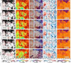 |
Fig. A.1. Inverted maps from STiC at log τc = 0.0, representative of the photosphere. From left to right: Vertical magnetic field strength, inclination, azimuth, LOS velocity, vLOS component, and temperature. The black contours indicate the size of the umbra, and the red contours mark the extent of the penumbra. The vertical dashed lines indicate where we made vertical cuts to analyze the vertical structure of the solar atmosphere. The magnetic field results are transformed to LRF. |
Appendix B: Details on the weak field approximation method applied in this study
The WFA allows for a first-order approximation of the magnetic field from the shape of Stokes I and any of the polarized Stokes components Q, U, or V. It returns a single value for the height range the given spectral line is sensitive to. Since the magnetic field is only approximated with a single parameter for each component, the investigated formation height range must fulfill the following criteria. The magnetic field should not change with depth, and it must be sufficiently weak, such that Zeeman splitting is well below the Doppler broadening of the spectral line,
 (B.1)
(B.1)
geff is the effective Landé factor of the spectral line, T the temperature and vmic the microturbulent velocity. M is the atomic mass of the species in question, k the Boltzmann constant, e0 and me the electron charge and mass, respectively, c the speed of light, and λ0 the center wavelength of the spectral line in question. The broad core of the chromospheric Ca II 8542 Å line fulfills these requirements for a large range of magnetic fields, making the WFA a widely used method for such diagnostics (see, e.g., de la Cruz Rodríguez et al. 2013; Kleint 2017; Centeno 2018; Kuridze et al. 2019). We used the neural field implementation of Díaz Baso et al. (2025) to compute the WFA. To prevent averaging over a larger depth than where the line core forms, we used a mask and excluded the wavelength points in the wings of the Ca II 8542 Å spectral line. This procedure prevents the strong signal from the photospheric wings from contaminating the chromospheric magnetic field estimate.
The main advantage of the implementation by Díaz Baso et al. (2025) is the spatial and temporal regularization scheme. Their approach allows one to train a function, fθ
 (B.2)
(B.2)
in the form of a neural network with trainable parameters θ at location x, y and time t to return the magnetic field components. The network is trained using the following loss function
![Mathematical equation: $$ \begin{aligned} \mathcal{L} _V=\sum _{x, y} \sum _\lambda \left[\left(-C_V B_{\parallel }(x, y \mid \theta ) \frac{d I_{x, y}^{\mathrm{obs} }}{d \lambda }\right)-V_{x, y}^{\mathrm{obs} }\right]^2, \end{aligned} $$](/articles/aa/full_html/2026/01/aa56465-25/aa56465-25-eq5.gif) (B.3)
(B.3)
and analogous loss functions for the Q, and U components are used to infer the perpendicular components of the magnetic field. B∥(x, y ∣ θ) refers to the solution from the neural field model, and the model is trained through gradient descent. This approach is generally called a physics-informed neural network (PINN) (Raissi et al. 2019; Karniadakis et al. 2021), and solves the inversion problem at the same time as the neural network is trained. Since the network takes the location of the pixel in question as input, it can only be used for the present observation. The network parameters converge after few iterations, and automatically regularize between pixels to some extent. To enhance the regularization in B⊥ and ϕ, they added an explicit regularization scheme to the loss function of the linear Stokes components, using a potential field extrapolation from the solution of B∥. The additional loss term is an ℒ2-norm between the BQ, U, and the potential field components Bpot, Q, U. This is different from the regularization scheme used, for instance, in Morosin et al. (2020), where they use an explicit regularization scheme between neighboring pixels. Comparing the two methods, we did not notice any substantial differences in the results.
All Tables
All Figures
|
Fig. 1. Overview of the evolution of NOAA active region AR13010 from May 15 – 17 with HMI. In the bottom left of each image is the timestamp of the HMI observation. The white square indicates the full FOV of CRISP. The black boxes on the right indicate the times at which we took SST observations. |
| In the text | |
|
Fig. 2. Detailed evolution of the sunspot. The upper panel displays the continuum intensity image for reference, and the lower panel shows the vertical magnetic field in the local reference frame. To cover the most important times of the penumbra formation, we display one HMI frame each hour between 08:00 and 12:00, and additionally one frame at 05:00, roughly three hours before the SST observations, and one frame at 14:00, roughly two hours after our last observation. The small black box indicates FOV selection, which we inverted with STiC. |
| In the text | |
|
Fig. 3. Overview image of the observation at 08:28 (upper set of panels) and 12:19 (lower set of panels). In each set of panels, the upper left panel shows the Hβ far wing image, the upper right panel the Hβ core forming in the chromosphere, the lower left panel shows the continuum image in Fe I 6302 Å and the lower right the line core of Ca II 8542 Å, also forming in the chromosphere. The black box indicates where we selected a subframe to invert the data with STiC. |
| In the text | |
|
Fig. 4. Milne-Eddington result maps showing the LOS magnetic field strength, B||, inclination, θ, azimuth, ϕB, and LOS velocity, vLOS, for the observation taken at 08:28 UT (upper panel) and 12:21 UT (bottom panel) for the 6302 Å line. The black contours indicate the extent of the umbra in the forming sunspot, while the red contours show the extent of the penumbra, which has formed by 12:21 UT in the southern sector. |
| In the text | |
|
Fig. 5. Chromospheric magnetic field inferred from the Ca II 8542 Å under the WFA. The panels show the LOS magnetic field strength (left) and the perpendicular magnetic field strength (right). The contours are identical to Fig. 4. |
| In the text | |
|
Fig. 6. Comparison between the vertical magnetic field in the LOS frame (upper panel) and the local reference frame (lower panel). The red and black contours indicate the size of the penumbra and umbra, respectively. The positive magnetic flux is only visible in the LOS frame, which may indicate projection effects. |
| In the text | |
|
Fig. 7. STiC inversion result maps (vertical magnetic field, Bz, LOS velocity, vLOS, and Fe I wing intensity) of the region of interest marked in Fig. 3. Dark red contours indicate where the vertical magnetic field exceeds 20 G, to better follow the evolution of the positive magnetic flux patch. Arrows are drawn to indicate the flow pattern of the emerging flux. Gray and black contours indicate the size of the penumbra and umbra, respectively. Within the area marked by the vertical dashed lines, the vertical structure of the atmosphere is analyzed in more detail. |
| In the text | |
|
Fig. 8. Temporal evolution of the vertical velocity (red) and vertical magnetic field strength (blue) at the location of maximum velocity as seen in the velocity maps of Fig. 6. The vertical dashed lines indicate the timestamps for which we present the results. |
| In the text | |
|
Fig. 9. Structure of the vertical magnetic field strength (left) and inclination (right) with height. The arrows indicate the direction of the magnetic field. The black contours in the left panel indicate the vertical magnetic field strength, while in the right panel, they display magnetic field inclination. The arrows indicate the direction of the magnetic field. In panels two to four, the emerging flux is visible as a positive patch of magnetic flux. |
| In the text | |
|
Fig. 10. Same as Fig. 9, but for the LOS velocity vLOS, and the horizontal magnetic field strength, Bh. In the left panel, the black contours show the vertical magnetic field strength, Bz, which is also depicted in the left panel of Fig. 9. The black contours in the right panel indicate the horizontal magnetic field strength, while the red contours indicate the vertical magnetic field strength. |
| In the text | |
|
Fig. A.1. Inverted maps from STiC at log τc = 0.0, representative of the photosphere. From left to right: Vertical magnetic field strength, inclination, azimuth, LOS velocity, vLOS component, and temperature. The black contours indicate the size of the umbra, and the red contours mark the extent of the penumbra. The vertical dashed lines indicate where we made vertical cuts to analyze the vertical structure of the solar atmosphere. The magnetic field results are transformed to LRF. |
| In the text | |
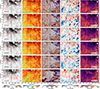 |
Fig. A.2. Same as Fig. A.1, but for log τc = −4.4, representative of the chromosphere. |
| In the text | |
Current usage metrics show cumulative count of Article Views (full-text article views including HTML views, PDF and ePub downloads, according to the available data) and Abstracts Views on Vision4Press platform.
Data correspond to usage on the plateform after 2015. The current usage metrics is available 48-96 hours after online publication and is updated daily on week days.
Initial download of the metrics may take a while.