| Issue |
A&A
Volume 705, January 2026
|
|
|---|---|---|
| Article Number | A179 | |
| Number of page(s) | 17 | |
| Section | Stellar structure and evolution | |
| DOI | https://doi.org/10.1051/0004-6361/202556543 | |
| Published online | 20 January 2026 | |
Convection signatures in early-time gravitational waves from core-collapse supernovae
1
Departament d’Astronomia i Astrofísica, Universitat de València, Dr. Moliner 50 46100 Burjassot, Spain
2
Observatori Astronòmic, Universitat de València 46980 Paterna, Spain
★ Corresponding authors: This email address is being protected from spambots. You need JavaScript enabled to view it.
; This email address is being protected from spambots. You need JavaScript enabled to view it.
; This email address is being protected from spambots. You need JavaScript enabled to view it.
Received:
22
July
2025
Accepted:
16
November
2025
Abstract
Context. Gravitational wave emitted from core collapse supernova explosions are critical observables for extracting information about the dynamics and properties of both the progenitor and the post-bounce evolution of the system. They are prime targets for current interferometric searches and represent a key milestone for the capabilities of next-generation interferometers.
Aims. This study aims to characterise how the gravitational waveform associated with prompt stellar convection depends on the rotational rate and magnetic field topology of the progenitor star.
Methods. We carried out a series of axisymmetric simulations of a 16.5 M⊙ red supergiant with five configurations of initial magnetic fields and varying degrees of initial rotation. We analysed the contribution of early-time convection and the proto-neutron star core to the waveform using ensemble empirical mode decomposition, alongside spectral and Fourier analyses, to facilitate the comparison and interpretation of the results.
Results. Our simulations show that the first six intrinsic mode functions dominate the early post-bounce gravitational wave signal, with variations due to rotation and magnetic fields influencing the signal strength. Strong magnetic fields decelerate core rotation, affecting mode excitation. Regardless of the initial rotation, convection consistently drives a low-frequency mode that lasts throughout the evolution.
Conclusions. We conclude that prompt convection can produce gravitational wave amplitudes comparable to or exceeding those of core bounce, with a persistent low-frequency component detectable in next-generation detectors.
Key words: convection / gravitational waves / magnetohydrodynamics (MHD)
© The Authors 2026
 Open Access article, published by EDP Sciences, under the terms of the Creative Commons Attribution License (https://creativecommons.org/licenses/by/4.0), which permits unrestricted use, distribution, and reproduction in any medium, provided the original work is properly cited.
This article is published in open access under the Subscribe to Open model. This email address is being protected from spambots. You need JavaScript enabled to view it. to support open access publication.
1. Introduction
Core collapse supernova (CCSNe) mark the terminal evolutionary stage of massive stars (MZAMS ≳ 8 M⊙). Throughout their lives, these stars undergo nuclear fusion, creating heavier elements up to the iron group. This process results in an onion-like structure, with an iron core at the centre, primarily supported by the pressure of relativistic degenerate electrons. When the core accumulates enough mass to exceed the Chandrasekhar limit, it begins to collapse (see e.g. Colgate & White 1966; Bethe 1990; Mezzacappa 2005; Kotake et al. 2006; Janka et al. 2007; Janka 2012; Burrows 2013; Melson et al. 2015; Lentz et al. 2015; Janka et al. 2016; Müller 2016, 2020; Burrows & Vartanyan 2021; Yamada et al. 2024). The density then rapidly increases, surpassing nuclear levels, setting the stage for the formation of a proto-neutron star (PNS). At this point, the collapse abruptly stops, causing the external layers, which are falling supersonically towards the stellar centre, to bounce and form a shock wave that propagates outwards into the infalling matter. Photodissociation of iron-group nuclei causes the shock to lose part of its energy, causing it to stall at ∼150 km. Various mechanisms have been proposed to explain the shock revival. The neutrino mechanism (Wilson 1982; Bethe & Wilson 1985), whereby 5 − 10% of the total outgoing neutrino luminosity from the PNS is deposited in the region behind the shock, is sufficient to revive the shock and drive the explosion in most cases. On the other hand, a small fraction of CCSNe can explode magneto-rotationally. In this latter case, fast rotation and strong magnetic fields enhance the energy deposition behind the shocked region, contributing to the creation of bipolar jets that drive an extremely energetic explosion (Bisnovatyi-Kogan et al. 1976; Mueller & Hillebrandt 1979; Symbalisty 1984; Akiyama et al. 2003; Kotake et al. 2004; Moiseenko et al. 2006; Obergaulinger et al. 2006; Burrows et al. 2007; Dessart et al. 2007; Winteler et al. 2012; Sawai & Yamada 2016; Mösta et al. 2014; Obergaulinger & Aloy 2017; Bugli et al. 2020).
Regardless of being the main driver of the explosion, neutrino emission and absorption in the post-shock region drive convection (Colgate et al. 1993; Herant et al. 1994; Fryer & Young 2007), which is suspected to create infalling funnels over the PNS and excite its oscillation modes (Vartanyan et al. 2023). Convection within the PNS also seeds these oscillations (Andresen et al. 2017; Mezzacappa et al. 2020, 2023; Murphy et al. 2025). Even though these explosion mechanisms have been extensively corroborated via theory and both 2-dimensional (2D) and 3-dimensional (3D) simulations (Mösta et al. 2014; Obergaulinger et al. 2014; Matsumoto et al. 2022; Vartanyan & Burrows 2023; Wang & Burrows 2024; Matsumoto et al. 2024), the direct detection of the multi-messenger CCSN signature in electromagnetic, neutrino, and gravitational radiation would mark a significant advancement in our understanding of these events (Kotake et al. 2012).
The current generation detectors such as Advanced LIGO (LIGO Scientific Collaboration 2015), Advanced Virgo (Acernese et al. 2014), and KAGRA (Akutsu et al. 2019) may detect the gravitational wave (GWs) emitted by a galactic explosion, and even more so with the next-generation ones such as the Einstein Telescope (ET) (Maggiore et al. 2020) and Cosmic Explorer (CE) (Reitze et al. 2019). GW detection offer a robust means of constraining the nuclear equation of state (EOS) (Malik et al. 2018; Raaijmakers et al. 2020), as has been demonstrated by the detection of the first binary neutron star (BNS) merger event, GW170817 (Abbott et al. 2017b). Beyond this GW also carry valuable information about the internal matter evolution during CCSN (Kuroda et al. 2016; Richers et al. 2017; Eggenberger Andersen et al. 2021; Murphy et al. 2024), making them one of the most valuable tools for studying the dynamics of the inner properties of these events.
Because of the stochasticity of their generation, GW signals from CCSNe pose significant challenges for analysis. Many processes contribute to their emission, from the oscillations caused by prompt convection in the early post-bounce phase, with frequencies of a few hundred Hertz (Marek et al. 2009; Murphy et al. 2009; Yakunin et al. 2010; Müller et al. 2013; Yakunin et al. 2015; Pan et al. 2018), to the f- and g-mode ramp-up signals whose frequencies rise to ∼1 kHz, driven by surface gravity modes of the PNS (Torres-Forné et al. 2018, 2019a; Bugli et al. 2023), and finally to ∼100 Hz features associated with the stationary accretion shock instability (SASI) (Blondin et al. 2003; Blondin & Mezzacappa 2007; Cerdá-Durán et al. 2013; Kuroda et al. 2016; Andresen et al. 2017; Mezzacappa et al. 2020, 2023). These processes are physically separated and provide complementary information: prompt convection is transient and stochastic, whereas later SASI or PNS-mode signals are coherent, quasi-periodic phenomena reflecting the longer-term hydrodynamic and structural evolution of the supernova core.
In this context, efforts to characterise GWs from CCSNe date back to the early 1980s (Mueller 1982; Zwerger & Mueller 1997), and have revealed a wide diversity of waveforms (see e.g. Dimmelmeier et al. 2002; Nakamura et al. 2016; Mezzacappa et al. 2023; Powell et al. 2023). Finally, Abdikamalov et al. (2014) and Richers et al. (2017) demonstrated that the GW bounce signal is primarily determined by the ratio of the rotational kinetic energy to gravitational energy (T/|W|) of the core at bounce.
In this study, we aim to characterise the GW signal associated with prompt convection in the early post-bounce phase as a function of the magneto-rotational properties of the collapsing core, as well as the influence of longer-term convective instabilities on GWs emission. Specifically, we explore how variations in rotational velocity and magnetic field strength affect the frequency, amplitude, and morphology of the resulting GW signal. Through systematic variation of these parameters in our simulations, we aim to identify correlations between physical core conditions and the emitted GW features.
This paper is organised as follows. Section 2 outlines our numerical set-up and presents the progenitor model and nuclear EOS used to perform the CCSN simulations. Section 3 describes the parameters used for the simulations and summarises the analysis methods employed in this work. In Section 4, we describe and present the main findings of our study. Section 5 discusses how the detectability varies with different rotation rates and magnetic field configurations. Finally, in Section 6 we draw our conclusions.
2. Model and numerical set-up
The axisymmetric simulations presented in this work were performed with the Aenus-ALCAR code (Obergaulinger 2008; Just et al. 2015, 2018), which solves the equations of special-relativistic magnetohydrodynamic (SRMHD) coupled with a multi-group neutrino transport two-moments scheme. To treat densities exceeding 8 ⋅ 107 g/cm3, we employed the SFHo EOS (Steiner et al. 2013) for dense nuclear matter. This EOS is broadly consistent with current astrophysical constraints, including those derived from NICER observations (Miller et al. 2019, 2021; Riley et al. 2019, 2021) and GW events (Abbott et al. 2017b, 2020a). Moreover, it accounts for neutrons, protons, electrons, positrons, and photons, as well as light nuclei (such as deuterium, tritium, and helium) and heavy nuclei in nuclear statistical equilibrium (NSE).
The effects of neutrinos during the simulation are treated in the two-moment framework closed by the maximum-entropy Eddington factor (Cernohorsky & Bludman 1994), with the inclusion of gravity in the neutrino transport equation following the 𝒪(v/c + ) formulation presented in Endeve et al. (2012). Neutrino-matter interactions consist of nucleonic absorption, emission, and scattering with corrections due to weak magnetism and recoil; nuclear absorption, emission, and scattering; inelastic scattering off electrons; pair processes (electron–positron annihilation), and nucleonic bremsstrahlung.
All the CCSN simulations presented in this work follow the evolution of the red supergiant stellar model s16.5. This model results from the spherically symmetric evolution of a progenitor star with MZAMS = 16.5 M⊙ (Sukhbold & Woosley 2014), solar metallicity, no rotation, and no magnetic fields. At the pre-collapse phase, the star retains only 14 M⊙, and the compactness of the core at 2.5 M⊙1 is 0.16.
Since the considered model is non-rotating, we superimposed an ad hoc rotation profile on the pre-collapse star (Eriguchi & Mueller 1985):
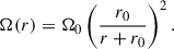 (1)
(1)
The radius r0 marks the location at which rigid (r < r0) transitions into differential rotation (r > r0). We set r0 = 1000 km in all models. Ω0 is the maximum initial rotation rate, and r is the spherical radius.
In a similar fashion, we added magnetic fields by initially introducing toroidal, Btor, and poloidal, Bpol, components at the pre-collapse phase of the supernova. We then define a field geometry with the vector potential A characterised by a typical distance R0 = 2 ⋅ 108 cm, (Suwa et al. 2007):
 (2)
(2)
All the models were simulated using spherical grids consisting of nθ = 128 zones in the θ direction, covering the whole polar domain θ ∈ [0, π] rad with a resolution of 1.4°. In the radial direction, we employ a logarithmically stretched grid with nr = 480 zones that extend from the centre of the domain to 1010 cm. This logarithmic stretching ensures an equal aspect ratio (i.e. Δr = rΔθ) of the cells down to a uniform resolution of 4 ⋅ 104 cm in the centre of the computational domain. In the energy domain, we used a logarithmically spaced grid with nϵ = 12 energy bins ranging from ϵmin = 0 MeV to ϵmax = 440 MeV.
Two models were also run at higher resolution (nr = 480, nθ = 256). Their results remain consistent with the standard-resolution runs, differing by less than ∼26% in the quantitative values of Section 4.3.
3. Simulations overview and analysis methods
3.1. Simulations overview
We performed 29 CCSN simulations starting from the red supergiant progenitor, s16.5 (see Section 2). In our models, we process the GW emission at run-time, producing outputs of the GW-strain and associated variables every 0.01 ms. We add rotation and magnetic field profiles using Equations (1) and (2), respectively. The range of central, pre-collapse rotation rate, Ω0, is [0, 2.4] rad ⋅ s−1, while the toroidal and poloidal components of the magnetic field span [0, 5] ⋅ 1011 G and [0, 1] ⋅ 1012 G. The values of the rotational rate and magnetic field strength are within the range usually encountered for models of massive stars in rapid rotation (e.g. Woosley & Heger 2006; Griffiths et al. 2022). Models in Table 1 are named following the format sA.B-C, where A.B denotes the value of Ω0 in rad ⋅ s−1, and C can be equal to 0, 1, 2, 3, or 4, reflecting increasing initial magnetic field strength (C = 0 denotes models without magnetic field).
List of models.
We output data every 1 ms, recording key physical quantities to analyse the link between the dynamics and the GW signal. For a refined analysis, models s0.0-1, s1.0-1, and s2.0-1 were rerun from 10 ms before bounce to at least 100 ms after, with an output cadence of 0.1 ms.
3.2. Analysis method
In this section we describe the methodology to identify contributions to the GW signal from different locations in our models (Section 3.2.1), the mathematical tool employed for the analysis of the GW signal, based upon ensemble empirical mode decomposition (EEMD) (Section 3.2.2), and the criterion employed to identify convective zones (Section 3.2.3).
3.2.1. Identification of the GW emission regions
The use of the approximate quadrupole formula (see Appendix A) allows us to identify contributions to the full GW signal by restricting the integral to subdomains inside the core. In the literature, similar decompositions have been employed, but these have mainly focused on subdividing the PNS interior itself (Andresen et al. 2017; Mezzacappa et al. 2023; Murphy et al. 2025). In contrast, here we compute the partial signals coming from three regions: (i) the PNS core (inside the PNS), (ii) the convective ‘sonic envelope’ (outside the PNS), and (iii) the outer region.
The actual definitions of these three regions follow. We define the PNS core as the region within the PNS where the entropy per baryon is smaller than 4 kB/bry. This value is commonly used in the literature to diagnose the explosion properties of pre-collapse stellar models (e.g. Ertl et al. 2016). The sonic envelope is the region in sonic contact with the centre (where |vr|< cs) excluding the PNS core. Moreover, to account for convective effects associated with rotationally driven matter transport, we extend the outer boundary of the sonic envelope by 20 km. Finally, the outer region is defined as the domain beyond the convective shell. The definitions of the above division are motivated by the characteristic frequencies of the resulting GWs emitted from each region as well as by the fundamentally different matter regimes in them (see also Section 4.1). Hereafter we will refer to the GWs emitted from the PNS core as ‘core strain’, from the sonic envelope as ‘sonic envelope strain’, and from the stellar region outside the sonic envelope as ‘outer strain’.
3.2.2. Ensemble empirical mode decomposition method
The empirical mode decomposition (EMD) is a method of decomposing a complex signal into a finite set of intrinsic mode function (IMFs), which represent simple oscillatory modes, as proposed by Huang et al. (1998a, 1999). Considering a signal, s(t), the first step of the algorithm involves identifying all the local maxima and minima within the signal. Using these points, an upper (lower) envelope is constructed by interpolating between the maxima (minima).
Once the envelopes have been calculated, their average is computed and then subtracted from the original signal. The result serves as a candidate for the intrinsic mode function (IMF). For a component to qualify as an IMF, it must satisfy two conditions: the number of extrema and zero crossings must either be equal or differ by at most one, and the mean value of the envelope defined by the local maxima and minima must be zero at any point (Flandrin et al. 2004).
The process, called ‘sifting’, is iterated by treating the IMF candidate as a new signal. The sifting continues until the IMF candidate changes negligibly between successive iterations or other stopping criteria are met, such as a predefined number of sifting iterations or a sufficiently low energy level in the residual signal.
After an IMF is extracted, it is subtracted from the original signal to obtain the residual. The residual then becomes the new signal, and the entire process is repeated to extract the subsequent IMFs. The algorithm stops when the residual is reduced to a monotonic function or one with no more extrema.
The EMD process results in the decomposition of the original signal as
 (3)
(3)
where ci(t) are the IMFs (k + 1 in the previous equation) and r(t) is the residual.
One of the major shortcomings of this method is mode mixing. To address this, Wu et al. (2009) proposed the EEMD. The algorithm is modified by adding white Gaussian noise to the original signal before calculating the IMFs and repeating this process n times. Finally, each ensemble is averaged to get the final IMFs. Thus two additional parameters are introduced: the ratio of the standard deviation of the Gaussian white noise to that of the original signal, σeemd, and the number of ensemble trials, n. By doing so, mode mixing is eliminated (or significantly reduced for a finite n), while the added white noise is averaged out through the ensemble mean.
The procedure we employed to decompose the GW signal into IMFs is as follows:
-
Filter the signal to remove all frequencies above 3000 Hz.
-
Perform standard EMD to obtain the IMFs and a residual.
-
Remove the residual from the filtered signal.
-
Perform EEMD, limiting the number of IMFs to 10, with σ0 = 1 and n = 2 × 10⁶.
To calculate the EMD and EEMD, we used the PyEMD package (Laszuk 2017) and the akima interpolation method (Akima 1970) to find the extrema.
Additionally, it is also possible to extract the instantaneous frequency (IF) of a single IMF, a sum of them, or the entire signal. The procedure, described in Huang et al. (1998b), consists of applying the Hilbert transform to the signal (or IMF). This allows for the construction of a composite signal whose real and imaginary components are the original signal and the Hilbert transform, respectively. Finally, by representing this complex signal in polar form, it is possible to determine its instantaneous phase, Φ(t), and to define the IF as
 (4)
(4)
3.2.3. Identification of convective regions
To locate convective zones in our models, we used the sign of the squared Brunt-Väisälä frequency, N2 (Obergaulinger et al. 2009; Gossan et al. 2020),
 (5)
(5)
where cs2 is the speed of sound, Φ the gravitational potential, and P the gas pressure. We evaluated N2 for each angle, θ, separately and identified convective zones by N2 < 0.
Additionally, we estimated the modulus of the convective velocity as
 (6)
(6)
where ⟨vi⟩Ω is the angular average of the velocity component i = r, θ, defined as
 (7)
(7)
Finally, from Equation (6) it is possible to derive the associated convection frequency as
 (8)
(8)
4. Results
To quantify the degree of rotation, we employed the sum of the rotational kinetic energies of the PNS core and sonic envelope divided by their gravitational energy, i.e. to the ratio T/|W| at core bounce. Specifically, in the following sections we identify models with T/|W|≤0.004 as slowly rotating, with 0.004 ≤ T/|W|≤0.010 as intermediately rotating2, with 0.010 ≤ T/|W|≤0.022 as fast-rotating, and finally T/|W|≥0.022 as very fast-rotating. The results of our simulations are summarised in Table D.1.
4.1. Qualitative overview
We first present a qualitative overview of the GW emission during the first 100 ms of post-bounce evolution, focusing on core bounce, PNS core vibrations, and convection. This analysis covers three representative pre-collapse rotation profiles: non-rotating (s0.0-1), intermediate (s1.0-1), and fast-rotating (s2.0-1). Unless otherwise noted, discussion of mode frequencies and spatial distributions refers to the last row of Figure 1, while the total, PNS core, sonic envelope, and outer strains are shown in the first, second, third, and fourth rows, respectively. In brackets we indicate the label of features in the last row of Figure 1 that can be associated with specific modes or other phenomena in the GW strain.
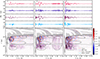 |
Fig. 1. Evolution of GW amplitude for models s0.0-1 (A), s1.0-1 (B), and s2.0-1 (C). Panels from top to bottom show the time evolution of the GW amplitude for the whole simulation domain, PNS core, sonic envelope, and outer layers. Finally, the bottom row shows the space-time evolution of 𝒟h(t, r). Dashed, solid, and dotted lines represent the PNS core, sonic envelope, and PNS average radius, respectively. Grey shades mark regions where N2 < 0, i.e. approximately, regions where convection takes place. Numbered ellipses identify GW modes in each region (see text). |
4.1.1. Core bounce
The PNS forms and abruptly halts the infalling matter, inducing vibrations in the core. At this stage, only the rotating models are sufficiently aspherical to produce significant GW emission. The emission cannot be neatly attributed to a single post-shock region. Instead, it originates from matter between r ≳ 12 km and the rapidly expanding, centrifugally deformed PNS surface, which, during this brief phase, coincides with the shock wave (1). This spatially extended emission produces the well-known pattern of an initial rise, a sharp minimum, and a subsequent maximum, lasting in total less than ≈5 ms, followed by lower-amplitude oscillations of similar period, as seen in the total waveform (best seen in the upper row of Figure 1C, corresponding to the model with the largest rotational rate).
4.1.2. PNS core vibrations
After bounce, the GW signal contains two identifiable components: one from oscillations of the PNS core and another from convection in the sonic envelope. These regions are not fully decoupled; they interact via hydrodynamic waves and convective penetration across their interface–often termed overshoot (outwards) or undershoot (inwards). In this section we introduce the contribution from PNS-core vibrations and discuss convection in Section 4.1.3.
As was noted in the previous section, all models exhibit prompt post-bounce core vibrations. Their aspherical components excite a high-frequency GW signal (f ≳ 500 Hz) that originates near the centre and propagates outwards (2, 3). These vibrations propagate with different frequencies before crossing the PNS core. High-frequency oscillations (f ≳ 1000 Hz) originate near the centre and propagate to r ∼ 10 km (2) before merging into lower-frequency components (f ∼ 750 Hz, 3), which then continue until they cross the PNS core. Upon crossing, these modes lose most of their energy and decrease their intensity, propagation velocity, and frequency (f ≤ 400 Hz, 4).
In the non-rotating model, the post-bounce configuration is nearly spherical, emitting GWs with negligible amplitude. Asymmetries are seeded by small deformations of the shock advected down to the core (5). After about 7 ms, non-spherical oscillation modes develop, and GW emission at f ≳ 500 Hz sets in. The oscillations, and corresponding GW signals, are stronger between t ≈ 15 ms and t ≈ 30 ms, but continue with generally lower amplitude for another ≈40 ms. In contrast, the PNS cores in rotating models are aspherical already when they form (see region (1) in Figures 1B,C). Their anisotropic oscillations emit ringdown modes immediately after bounce.
The intermediate-rotation model maintains noticeable oscillations throughout the entire 100 ms interval displayed in Figure 1B, though with reduced intensity near 50 ms and 100 ms. After an initial stabilisation, rotation re-excites the core around 60 ms post-bounce. The resulting oscillations propagate outwards at the sound speed (cs ∼ 4–9 ⋅ 109 cm s−1). They experience slight damping when entering the small convectively unstable region outside the core (shaded around r ≈ 20 km), but reappear clearly farther out as vertical stripes spanning both core and sonic envelope. This re-excitation occurs when the epicyclic frequency (or one of its overtones) of fluid layers around the core matches a specific mode, leading to resonance (see Cusinato et al. 2025). In this case, a mode near 750 Hz is excited (6).
The fast-rotation model does not show renewed activity after t ∼ 40 ms. The absence of re-excitation can be explained by rotational suppression of core deformations, consistent with earlier studies (Dimmelmeier et al. 2008; Shibata & Sekiguchi 2005).
In all cases, the core strain retains a high characteristic frequency. Its amplitude decreases in all models except the intermediate-rotation case, where resonance amplifies it (Cusinato et al. 2025), consistent with the findings of Westernacher-Schneider et al. (2019).
4.1.3. Convection
Following bounce, negative entropy and Ye gradients develop in the sonic envelope, triggering prompt convection in both non-rotating (Bruenn & Mezzacappa 1994) and rotating models. This phase lasts until about 25 ms, during which the convective region spans most of the sonic envelope and extends below the PNS core boundary. The instability criterion, N2 < 0, shown in Figure 1 only approximates this behaviour: convection begins where the squared Brunt–Väisälä frequency becomes negative (the shaded region), but quickly overshoots inwards, nearly reaching the core.
The resulting strong, chaotic fluid motions last up to ∼40 ms and produce positive and negative  with large amplitude in the sonic envelope (7). Eventually, the radial extent of the convective layer shrinks. Typical frequencies are f ≲ 500 Hz. As prompt convection subsides, activity retreats to the outer edge of the sonic envelope, producing weak advection modes that propagate inwards (8).
During this phase, the sonic-envelope strain dominates the overall emission, with a pronounced peak around 10 − 20 ms followed by weaker activity. Its intensity is comparable in fast- and slow-rotating models, but enhanced in the intermediate case.
Throughout the evolution, the outer-region strain remains comparatively weak, reflecting mainly the overshooting motions of prompt convection above the sonic envelope and centrifugal effects on infalling matter. Slower equatorial infall (relative to the axis) produces a quadrupole mass moment and thus weak emission. This effect grows with rotation rate.
4.2. GW ensemble empirical mode decomposition
After removing the residuals (see point (iii) of Section 3.2.2), we decomposed our filtered waveforms into 10 IMFs as is described in Section 3.2.2. We used the matching score, M, as a metric to determine which of the IMFs contribute to the overall waveform (Suvorova et al. 2019):
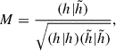 (9)
(9)
where h is the original signal with the EMD residual removed,  is the signal obtained by summing a certain number of IMFs, and (a|b) denotes the inner product.
By analysing the matching score, we notice that the first two and the last two IMFs contribute negligibly to the strain. The former are associated with high-frequency numerical noise, while the latter are too weak to be significant components of the original signal. Hereafter, we identify the first significant IMF (sIMF) as the third one produced by the process (see Figure 2 for the signal decomposition into sIMFs). Moreover, the matching coefficient exceeds 0.95 in every case. Therefore, we conclude that the overall GW strain is consistently approximated by the first six sIMFs.
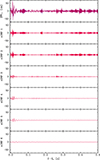 |
Fig. 2. Time evolution of the total GW strain and the six sIMFs for model s1.2-1. The dashed blue line on the first panel represents the full strain extracted on the whole simulation domain, and the solid red line the strain as a sum of the sIMFs. |
In the case of jet formation, the outflow of ejected matter causes the GW signal to drift to positive values (see e.g. the case of models s1.0-4 and s1.8-4 in Figure D.1). This drift translates into a non-periodic signal enclosed in the residual of the EMD. For this reason, we remove the residual from the waveform to obtain a signal that oscillates around zero.
Following the qualitative observations made in Section 4.1, and particularly the observation on the characteristic frequencies of the strain in each of the analysis regions, we find that the core strain is well approximated by sIMFs 1, 2, and 3, while the convective part of the strain corresponds to sIMFs 4, 5, and 6. Using the matching coefficient to probe the alignment between this prescription and the strain extracted from the hydrodynamic quantities, we find that it is above 0.6. This lower matching score is likely a result of the fact that modes are not strictly confined to the regions where they originate; rather, they can propagate into or influence neighbouring regions (e.g. fast modes generated in the PNS core and propagating through the sonic envelope). From now on, we refer to the sum of the first three sIMFs as PNS core strain, hcore, and to the sum of the last three after the bounce time (which we conventionally take as 5 ms) as convection strain, hconv.
4.3. Bounce and convection signals
For the models with magnetic field configuration 1 (sA.B-1 in Table 1), the loudest signal of the early post-bounce waveform (t ≲ 100 ms) is, depending on the rotation rate, either the bounce signal or the strong peak due to convection that appears within the following 20 ms. We compute the difference between the highest and lowest points in the bounce signal (t ≤ 5 ms), Δhb, and the post-bounce signal (5 ms ≤ t ≤ 100 ms), Δhpb.
Figure 3A shows these differences as a function of T/|W|, at core bounce. As is described in Abdikamalov et al. (2014) and Richers et al. (2017), the bounce signal, at the rotation rates we are considering, depends linearly on T/|W|, and the slope obtained from a linear regression of our models agrees within 5% with the prediction of Richers et al. (2017) for the SFHo EOS and corresponding T/|W| values. On the contrary, Δhpb fluctuates between 70 cm and 200 cm as T/|W| increases, with its lowest and highest values occurring when T/|W| is 0.003 and 0.007, respectively. Additionally, we observe that for slow and intermediate rotational rates, the magnitude of the post-bounce signal varies more significantly and also dominates over the magnitude of the bounce signal. In contrast, for fast rotation regimes, the magnitude of the post-bounce signal remains relatively unchanged across different values of T/|W|.
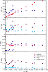 |
Fig. 3. Panels A and B show the difference between the highest and lowest points of the GW signal, Δh, against the rotational kinetic energy to gravitational energy ratio for bounce and post-bounce signals, and for PNS core (Δhcore) and convection (Δhconv) signals, respectively, for models with magnetic field configuration 1. Panels C and D display the frequencies of the previous intensity peaks in relation to the same quantity on the x axis for the same pool of models as in the previous two panels. |
As is observed in Section 4.1, the post-bounce signal comprises different modes oscillating at various frequencies. Therefore, the oscillations in magnitude can be attributed to their constructive or destructive interference. To better understand this, in Figure 3B we separately study the intensity of the signals arising from the convection, Δhconv, and PNS core, Δhcore, as sums of their corresponding sIMFs (see Section 4.2). For the entirety of our sample, the convection signal reaches the maximum strain width around 15–20 ms (Figure 3B), which indicates that prompt post-bounce convection causes the strongest GW signal in the convective strain. After the bounce, gradients in entropy and lepton fraction form due to the weakening shock and core deleptonisation, driving the build-up of convective bubbles surrounding the PNS core (see Figure 4A). Convective motions cause the GW amplitude to grow but also tend to flatten the entropy and electron fraction gradients. When this happens, the GWs amplitude growth stops. Before convection ceases, it reaches its maximum strength, marked by the peak in Δhconv and its associated GW signal. Moreover, we see that the convection strain range width, Δhconv, is maximum for very slowly rotating progenitors and for a specific value of T/|W| = 0.007, while it drops to around 40 cm for all other configurations (Figure 3B).
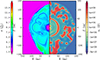 |
Fig. 4. Panel A: Snapshot of the entropy at 15 ms after bounce, showing the convective bubbles surrounding the PNS core. Panel B: Snapshot of the radial velocity at 65.7 ms, showing the propagation (here at 50 km) of a wave generated by oscillations of the PNS core and propagating outwards. Both snapshots are for model s1.0-1. |
In most cases, the maximum of the strain range width of the PNS core GW, Δhcore, and that of the convective strain are nearly coincident (Figure 3B, for T/|W|≈0.007). This is another manifestation of the resonance between the epicyclic frequency and the core normal oscillation modes found in Cusinato et al. (2025). While Δhcore is mild at low rotation rates, it peaks at intermediate ones, and then stabilises at around 90 cm in the faster rotating models, when it also becomes the part of the waveform with the larger amplitude. Notably, the strain range width of the core and convective strain resonates (Cusinato et al. 2025) at the same rotation rate (at around T/|W|≈0.007; Figure 3B).
In Figures 3C and 3D, we display the dominant frequency for the bounce (fb), post-bounce (fpb), PNS core (fcore), and convective (fconv, peak) signals as a function of T/|W| at bounce (see Appendix B). The peak frequency for the bounce signal shows little variation with increasing rotation (Figure 3C) as discussed by Richers et al. (2017). However, fb stabilises in our models at ∼500 Hz, whereas in their case this plateau is at ∼700 Hz. This discrepancy can be attributed to the different treatment of gravity or to the difference in the employed progenitor model. On the other hand, fpb behaves differently in three different regimes. In slowly rotating models, convection dominates the GW signal over the PNS ringdown oscillations and PNS core vibrations. Hence, the dominant frequency is that of convection, i.e. 150–200 Hz. In intermediately rotating models, rotation causes the excitation of fast oscillating modes that in most cases dominate the GW signal over convection, though some cases are convection-dominated. In models with fast and very fast rotation, the bounce is violent enough to produce strong intensity ringdown oscillations, with a frequency similar to that of the bounce signal.
Similarly to the intensity peaks, we also separately analyse the peak frequency of the convection and PNS core signals. The convection signal peak frequency settles at ∼150 Hz regardless of the model’s pre-collapse rotation (Figure 3D), indicating that prompt convection is not significantly affected by it. On the contrary, the PNS core peak frequency shows a non-monotonic dependence on the rotation rate, varying from 250 Hz to 900 Hz for most of the considered models.
Slowly rotating models with T/|W|∼0 and intermediate rotating models show the highest frequency peaks, but for two different reasons. The former show high-frequency modes excited by the strong convection formed post-bounce, while the latter’s modes are excited in resonance with the rotation (see the peak of both Δhconv and Δhconv at around T/|W|≈0.07 in Figure 1B). On the other hand, fast and very fast-rotating models exhibit only the ringdown oscillations from the bounce signal, with a decreasing trend fcore as rotation increases.
4.4. Time evolution
We considered the overall evolution of the waveform for models with the standard magnetic fields configuration (labelled as 1), for which rotation has a major dynamic impact. Particularly, with faster rotation, the PNS deforms, flattening at the poles and bulging at the equator due to centrifugal force. Rotation also effectively suppressing the PNS core vibrations by dampening external excitations of PNS vibrations (Pajkos et al. 2019).
Figure 5 shows the GW time evolution and corresponding spectrograms for three models (s0.4-1, s0.9-1, and s2.4-1), each representative of a different rotational range. Regardless of the initial rotation, the GWs emission is highly active from bounce until approximately 25 ms post-bounce across a broad frequency spectrum. As described in Section 4.1, this phase is characterised by strong prompt convection, emitting both low-frequency (f ≲ 500 Hz) and high-frequency (f ≳ 500 Hz) GWs. A notable feature in the high-frequency category is a mode at 750 Hz, which intensifies with increasing rotation rate (see Figure 5, bottom panels). In slow, fast, and very fast-rotating models, high-frequency modes weaken and disappear after ∼50 ms. The GW emission then enters a quieter phase, characterised by a smaller amplitude and a steady increase in the frequency.
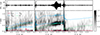 |
Fig. 5. GW amplitude (top row) and corresponding spectrograms for models s0.4-1 (panel A, representative of the class of slowly rotating models), s0.9-1 (B, prototype of intermediately rotating cases) and s2.4-1 (C, representative of the class of fast-rotating models), calculated with a time window of 10 ms. The red line corresponds to the convection frequency (Equation (8)) at the sonic envelope surface, the blue lines show the epicyclic frequency (solid) and its first overtone (dotted) in the π/4 direction at the PNS core surface, while the green line is the fundamental quadrupolar mode frequency (2f) computed with the quasi-universal relation in Torres-Forné et al. (2019b). |
The behaviour of the intermediately rotating case is exceptional. The frequency of the mode excited due to rotation starts to ramp up as well (see bottom panel of Figure 5B). Additionally, in all rotational regimes, mode mixing renders the fundamental 2f mode (Torres-Forné et al. 2019b; Rodriguez et al. 2023, green lines) and the convection modes indistinguishable in the spectrograms. Nevertheless, a cautionary note is in order here. Since the frequency of the fundamental 2f mode has been obtained from universal relations computed for non-rotating CCSN simulations, and their applicability to fast-rotating cases is not direct, the actual evolution of the 2f may be somewhat different from that presented in this paper.
At timescales longer than ≈25 ms, the low-frequency GW signal is no longer associated with prompt convection. Instead, it originates from longer-lived convective activity in the post-shock region, which we characterise through the Brunt–Väisälä frequency (Equation (5)). For clarity, we will refer to this later signal as ‘convection’, while the early-time contribution will be explicitly denoted as ‘prompt convection’. It is also worth noting that, on similar timescales, additional non-convective contributions such as SASI may also produce low-frequency GW emission (see e.g. Kuroda et al. 2016; Andresen et al. 2017; Mezzacappa et al. 2023).
For slowly and intermediately rotating models, the broadband interval of frequencies associated with the 2f mode gradually separate from the convection mode between 0.1–0.2 s, reaching frequencies between 700–1000 Hz at 0.5 s post-bounce (bottom panels of Figures 5A and 5B). On the contrary, in fast- and very fast-rotating models, the separation between convection and normal modes is delayed in the spectrogram (see Figure 5C), beginning around t ≥ 0.2 − 0.3 s post-bounce, and even then the distinction remains less pronounced than in slower rotations (bottom panel of Figure 5C). This delay can be attributed to strong centrifugal forces, which, in very fast-rotating axisymmetric models, slow down the PNS contraction and oscillations. Afterwards, the frequency broadens, spanning lower ranges (0–700 Hz) but with reduced intensity. It should be noted that the universal relations predicting the 2f mode frequency were derived from non-rotating configurations (Torres-Forné et al. 2019b). Therefore, some discrepancies between the predicted and observed 2f-mode frequencies may arise in the most rapidly rotating configurations.
After the crossing with the 2f mode, convection modes maintain a steady frequency at ∼100 Hz. In slow and intermediate rotation cases, these modes tend to strengthen beyond ∼0.3 s, while in fast and very fast rotations they diminish over time.
In intermediately rotating models, rotation resonates with specific PNS modes, exciting them (Cusinato et al. 2025). To characterise the frequency of fluid element oscillations in the cylindrical radial direction within our rotating PNS, we use the epicyclic oscillation frequency:
 (10)
(10)
where n is the overtone number and κ is the epicyclic frequency, defined as
 (11)
(11)
with R being the cylindrical radius. Specifically, we employed the average of the local maxima of this quantity in a conical region spanning [15° , 85° ] inside of the PNS core.
In the intermediately rotating models, a mode at 750 Hz, excited during bounce, resonates with the fundamental epicyclic frequency (solid blue line in the lower panel of Figure 5B), producing multiple GW bursts of varying amplitudes, of which the most noticeable appears at 0.30–0.45 s (see also e.g. the first two rows of Figure 1B at 0.06–0.09 s). These bursts result from a resonance between PNS core oscillations and the rotational frequency (see Figure 4B). When the fundamental epicyclic frequency crosses the 2f mode, it resonates with it, leading to an increase in GW amplitude to values comparable to Δhpb around ∼0.3 s that lasts until the end of the simulation (top panel of Figure 5B). Additionally, soon after this time, the first overtone of the epicyclic frequency excites a mode at 1500 Hz. The energy carried by GWs decreases as rotation increases. However, in intermediate rotation models, the resonance between the PNS modes and rotation breaks this trend and leads to a higher energy emission (see e.g. EGW, 300 and EGW columns in Table D.1). In all models, the dominant mode remains the fundamental 2f mode regardless of the initial rotation.
Using Equation (9), we compare the 2f-mode characteristic frequency obtained with the universal relations in Torres-Forné et al. (2019b) with the IF from the sum of the first three sIMFs. Our models consistently yield a matching score above 0.91, confirming that the rotation rates considered here do not induce significant deviations.
Finally, Figure 6 compares the IF derived from the convection strain and fconv, calculated as the mean value of Equation (8) within a region extending from 15° to 165° in colatitude and radially form 30 km above to 30 km below the sonic envelope boundary for model s0.4-1. This angular range avoids axis-related interference, while the radial bounds have been chosen to capture the full effect of convection. Using Equation (9) for both frequencies yields a matching score above 0.7 for all models, except for slow and intermediate rotating strongly magnetised rotating models (s0.6-4 and s1.0-4) which have a score of 0.45 and 0.5, respectively.
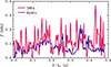 |
Fig. 6. Evolution of the frequency of the convection strain expressed as the IF of the sum of the last three sIMFs (blue line) and as the frequency associated with the convective velocity for model s0.4-1. |
4.5. Effect of magnetic fields
For three of the four regimes that we identified – slow rotation, intermediate rotation, and fast rotation – in addition to the standard pre-collapse magnetic field configuration (labelled as 1), we ran four more models with different initial magnetic field configurations. The additional configurations are non-magnetised (0), or possess ten (2), a hundred (3), and a thousand times (4) the initial field strength.
4.5.1. Bounce and convection signals.
The magnetic field configuration, particularly at higher strengths, significantly affects the evolution of T/|W|. Figure 7 shows the time evolution of T/|W| during the first 100 ms for the four configurations of model s1.0. While T/|W| peaks at bounce time in all cases, configurations 0 through 3 exhibit similar peak values. In contrast, the peak value of configuration 4 shows fluctuations as the rotation varies. It decreases in models with slow and intermediate rotations but increases in the fast-rotating model compared to their respective reference configurations (see T/|W| column in Table D.1).
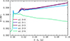 |
Fig. 7. Evolution of the first 100 ms of the total rotational kinetic energy of PNS core and sonic envelope divided by the total gravitational energy for the four magnetic field configurations of model s1.0. |
The post-bounce evolution follows a consistent trend across rotation rates: T/|W| for configurations 0 to 3 increases rapidly until approximately ∼15 ms. Afterwards, the rate of increase slows, with configuration 3 experiencing the slowest growth. On the contrary, configuration 4 behaves differently due to magnetic braking, which decelerates the core thus lowering T/|W|.
The bounce strain range width and frequency are not significantly affected by the strength of the magnetic fields (see Δhb in Table D.1), as magnetic braking does not have sufficient time to influence core rotation. However, the magnetic field affects how the post-bounce, core, and convection range widths depend on the rotation rate. In the slow and fast-rotating models, most values of Δhpb, Δhcore, and Δhconv, along with their associated frequencies for all magnetic field configurations, remain close to the reference values (see Table D.1). However, configurations 0 and 3 for model s0.6 show a stronger strain range width. This discrepancy arises from a higher degree of asymmetry in the location of the convective bubbles forming during the prompt convection phase (e.g. similar to the ones shown in Figure 4B). For the intermediate rotation model, the range strain widths and frequencies span a broader range of values depending on the magnetic field strength. This occurs because the system is in a resonant regime, where small changes due to the magnetic fields changing the dynamics can either enhance or weaken the resonance.
4.5.2. Time evolution.
We find that in non-magnetised models (configuration 0), the waveform evolution resembles that of models with the standard configuration, regardless of the initial rotation rate, suggesting that the magnetic fields of the standard configuration are too weak to significantly alter the dynamics.
In the following, we focus on models in which stronger fields cause major differences from the cases discussed above in Section 4.4. Figure 8 compares the time evolution and corresponding spectrograms of GWs for magnetic field configuration 4 in models s0.6, s1.0, and s1.8. The spectrograms were computed by removing the residual from the original signal, so that the convection signature is not masked by the low-frequency memory signal associated with the jet structure.
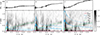 |
Fig. 8. Same as Figure 5 but for models s0.6-4, s1.0-4, and s1.8-4. The residual was removed to prevent the low-frequency memory signal from masking the convection signal. |
In the stronger magnetised models (configurations 2, 3, and 4), rotation amplifies the magnetic field along the symmetry axis, leading to jet formation. These polar jets begin forming at around 200 km from the centre, with their formation timescale largely determined by the strength of the initial magnetic field components. Moreover, mildly relativistic matter moving within the jets causes a slow shift of the GW signal to positive values (top panels of Figure 8). This memory effect becomes particularly significant when the jets are well developed, extending to approximately ∼800 km from the star’s centre, and widens progressively as the jets propagate outwards. Additionally, stronger initial magnetic fields and faster rotation rates result in a greater deviation of the GW signal from zero.
For the intermediate-rotation case, magnetic braking in configurations 0 through 3 is sufficient to significantly slow down the core, allowing for the same resonance with the epicyclic frequency or one of its overtones observed before. However, the strong magnetic fields in configuration 4 cause substantial magnetic braking, slowing down the core. Therefore, the epicyclic frequency no longer coincides with the PNS core vibrations responsible for high-frequency bursts of GWs in the post-bounce phase, resulting in the disappearance of these vibrations after ∼50 ms (top panel of Figure 8B).
On the contrary, for the strongly rotating model s1.8, the magnetic braking due to the strong fields in configuration 4 slows the PNS core sufficiently for the epicyclic frequency and its first overtone to cross the 2f mode frequency at ≃200 ms and ≃420 ms after bounce, respectively (Figure 8C). These mode crossings imprint moderate-amplitude oscillations, which are much smaller than in model s0.9-1.
By significantly slowing down the PNS core, the magnetic field configuration 4 reduces the energy emitted as GWs by the intermediate-rotation model during the post-bounce phase compared to the cases with weaker fields. Among the fast-rotating models, the one with the strongest field emits the most energy (column EGW, 300 in Table D.1).
Additionally, in the bottom panels of Figure 8, we plot fconv as approximated by Equation (8). For the intermediate and slow rotating models with magnetic field configuration 4, we observe that the frequency of the convective strain tends to be lower compared to their less magnetised counterparts. We attribute this behaviour to strong magnetic fields hindering convection.
We conclude this section by checking whether the usefulness of the IF as a tool for identifying the convective dynamics is affected by the presence of magnetic fields. We find support for this assumption in the form of a matching score between the last three sIMFs and the fconv derived from the hydrodynamic variables, calculated using Equation (9), above 0.6 for all models except for s1.0-0 and s0.6-4, where the match is reduced to 0.4 and 0.5, respectively.
5. Discussion
5.1. Prospects of detection
By comparing panels A, B, and C of Figure 9, which show a slow (A), an intermediate (B) and a fast-rotating progenitor (C), we notice that a strong (broad-band and strongly time-localised) signal comes from the early post-bounce convection and ringdown in the slow and intermediate rotators, while in the fast rotator, the most prominent signal comes from the bounce. Due to the PNS ringdown oscillations, the combination of frequencies of these two signals is very similar, posing a challenge in determining the precollapse rotation of the progenitor in the event of a GW detection from a CCSN. Moreover, we observe that models with higher GW energy emitted during the bounce or post-bounce phase (see Table D.1 and Appendix C for the details of the analysis) can be observed at higher distances.
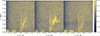 |
Fig. 9. Time-frequency diagrams of the GW strain at 10 kpc injected into Gaussian noise for models s0.2-1 (panel A), s0.9-1 (panel B) and s1.8-1 (panel C), as seen by the LIGO Livingston interferometer for an event occurring at RA 16.99 h, Dec −35.59° and arrival time 1393213818 s. |
The inference of  is more challenging than the bounce signal due to the large variety of modes that play a role in the waveform and the much weaker signal produced. With an emitted energy of ≲1045 erg (see EGW, pb in Table D.1), the signal emitted by very fast-rotating CCSNe after the post-bounce peak is too weak to be detected even in events happening as close as 1 kpc. The possibility of detections reported in models such as s2.0-1 and s2.4-1, at higher distances, is likely a false positive of the Gaussian noise.
Progenitors with slow and fast initial rotation can be well reconstructed, at least for the best scenario, until 30 kpc. Finally, most of the intermediate rotating models, even if they generally emit more energetic GWs, due to the presence of resonant modes, can only be partially recovered. This is because, especially in the early post-bounce phase, the higher frequencies excited by resonance can interfere with the mode tracking, leading to an incomplete recovery.
If, instead of the current generation detectors, we used third-generation interferometers such as the ET and CE, located at the current Virgo and LIGO sites, respectively, with their theoretical sensitivity (Hild et al. 2011; Abbott et al. 2017a), the results would improve significantly: the bounce signal of all models can be recovered with at least one detector for the best scenario. While  remains hard to infer for very fast-rotating progenitors, detection for all other configurations improves, allowing for a good match until 70 kpc. Moreover, the better sensitivity allows for a better resolution of the modes even in resonating cases, leading to a good inference of
  for these models.
5.2. Limitations of this study
This study has several limitations, which could impact the generalizability and applicability of the results. The first one arises from considering only 2D CCSN simulations, which produce only one GW strain polarisation, h+. This restriction limits our ability to fully characterise the GW signals, as real astrophysical events occur in three dimensions (3D) and typically generate two independent GW polarisations. Therefore, the findings derived from these 2D simulations might not accurately represent the complexities and nuances of actual CCSN events. Additionally, it is already well known that axisymmetric simulations tend to overestimate the amplitude of the waveform.
Moreover, our study only considered a single red supergiant progenitor model. This model was evolved through the main sequence without rotation and had a standard compactness at the pre-collapse stage. Limiting the study to one progenitor model restricts the scope of our conclusions, as different progenitor characteristics, such as initial mass, metallicity, and compactness, can significantly influence the dynamics of the collapse and the resulting GW signals. By not incorporating a broader range of progenitor models, we may overlook the potential variability and diversity in GW signals that could arise from different stellar evolution pathways.
Adding a magneto-rotational profile to a non-rotating progenitor is not necessarily physically consistent. There is a clear interplay between rotation and magnetic fields, which directly impacts the stellar structure. However, the lack of sufficiently detailed grids of pre-supernova models covering both realistic core rotation rates and magnetic field strengths limits our ability to use fully self-consistent progenitors. Parametrising rotation and magnetic fields as in Equations (1)and (2) enables us to systematically explore how each of these physical ingredients influences the gravitational wave signal. More realistic stellar progenitors – including rotation and magnetic fields in a self-consistent way – would likely introduce more complex dependencies in the GW signal, which are beyond the scope of this study.
6. Conclusion
We have presented 29 axisymmetric CCSNe simulations based on a single red supergiant progenitor star, systematically exploring a range of magnetic field configurations and rotation profiles. Our goal was to investigate the connection between GWs and hydrodynamic convection during the early post-bounce times.
Our analysis reveals that the GW signal can be effectively approximated using the first six sIMFs derived from EEMD on the raw GW strain. Specifically, the first three sIMFs reflect the contribution from the PNS core, as well as the 2f mode, while the last three are associated with the sonic envelope and its surrounding convective activity. The large matching scores obtained in both cases reinforce the reliability of EEMD as a tool for extracting physically meaningful information from GW data related to the source dynamics.
For slowly and intermediately rotating models, we observed that the bounce signal is not consistently the dominant component of the waveform. Instead, the post-bounce signal, typically resulting from the interference between PNS ringdown oscillations and prompt convection, becomes more prominent. In progenitor models with pre-collapse rotation rates near 1 rad ⋅ s−1, both convection and PNS core vibrations are strongly excited, resulting in the loudest post-bounce signals seen in our simulations.
Furthermore, we confirm the results anticipated in Cusinato et al. (2025) that rotation leads to an enhancement of the post-bounce signal over longer timescales, caused by the resonant excitation of mode frequencies near the PNS core boundary. This resonance boosts the GWs energy emission, with an observed strain amplification of approximately one order of magnitude.
Across all explored configurations of rotation and magnetic fields, we consistently found that convection produces a low-frequency mode persisting throughout the evolution. This mode is closely correlated with the frequency of convective velocity at the outer radius of the sonic envelope. We point out that the identification of this mode can be performed employing suitable sIMFs resulting from an EEMD of the GW data.
Our work further highlights the impact of strong magnetic fields. In addition to inducing jet formation and causing a GW memory offset, strong magnetic fields also decelerate core rotation. This deceleration either suppresses the resonance-induced modes in intermediately rotating models or triggers similar resonances in initially fast-rotating models as they spin down.
Acknowledgments
We acknowledge support from grant PID2021-127495NB-I00 funded by MCIN/AEI/10.13039/501100011033 and the European Union, as well as from the Astrophysics and High Energy Physics programme of the Generalitat Valenciana (ASFAE/2022/026), funded by MCIN and the European Union NextGenerationEU (PRTR-C17.I1), and from the Prometeo excellence programme grant CIPROM/2022/13 funded by the Generalitat Valenciana. MC acknowledges the support through the Generalitat Valenciana via the grant CIDEGENT/2019/031. MO was supported by the Ramón y Cajal programme of the Agencia Estatal de Investigación (RYC2018-024938-I). We are grateful to Tristan Bruel for providing the PNSinf pipeline. The computations have been performed on servers Lluisvives and Tirant-4 (grant AECT-2025-2-0002) of the Servei d’Informàtica de la Universitat de València and on the Red Española de Supercomputación (RES) on MareNostrum (grants AECT-2025-1-0012 and AECT-2025-2-0006).
References
- Abbott, B. P., Abbott, R., Abbott, T. D., et al. 2017a, Class. Quant. Grav., 34, 044001 [NASA ADS] [CrossRef] [Google Scholar]
- Abbott, B. P., Abbott, R., Abbott, T. D., et al. 2017b, Phys. Rev. Lett., 119, 161101 [Google Scholar]
- Abbott, B. P., Abbott, R., Abbott, T. D., et al. 2020a, ApJ, 892, L3 [NASA ADS] [CrossRef] [Google Scholar]
- Abbott, B. P., Abbott, R., Abbott, T. D., et al. 2020b, Liv. Rev. Relat., 23, 3 [NASA ADS] [Google Scholar]
- Abdikamalov, E., Gossan, S., DeMaio, A. M., & Ott, C. D. 2014, Phys. Rev. D, 90, 044001 [Google Scholar]
- Acernese, F., Agathos, M., Agatsuma, K., et al. 2014, Class. Quant. Grav., 32, 024001 [Google Scholar]
- Akima, H. 1970, J. ACM, 17, 589 [Google Scholar]
- Akiyama, S., Wheeler, J. C., Meier, D. L., & Lichtenstadt, I. 2003, ApJ, 584, 954 [NASA ADS] [CrossRef] [Google Scholar]
- Akutsu, T., Ando, M., Arai, K., et al. 2019, Nat. Astron., 3, 35 [NASA ADS] [CrossRef] [Google Scholar]
- Andresen, H., Müller, B., Müller, E., & Janka, H. T. 2017, MNRAS, 468, 2032 [NASA ADS] [CrossRef] [Google Scholar]
- Bethe, H. A. 1990, Rev. Mod. Phys., 62, 801 [CrossRef] [Google Scholar]
- Bethe, H. A., & Wilson, J. R. 1985, ApJ, 295, 14 [CrossRef] [Google Scholar]
- Bisnovatyi-Kogan, G. S., Popov, I. P., & Samokhin, A. A. 1976, Ap&SS, 41, 287 [NASA ADS] [CrossRef] [Google Scholar]
- Blondin, J. M., & Mezzacappa, A. 2007, Nature, 445, 58 [CrossRef] [PubMed] [Google Scholar]
- Blondin, J. M., Mezzacappa, A., & DeMarino, C. 2003, ApJ, 584, 971 [NASA ADS] [CrossRef] [Google Scholar]
- Bruel, T., Bizouard, M.-A., Obergaulinger, M., et al. 2023, Phys. Rev. D, 107, 083029 [Google Scholar]
- Bruenn, S. W., & Mezzacappa, A. 1994, ApJ, 433, L45 [Google Scholar]
- Bugli, M., Guilet, J., Obergaulinger, M., Cerdá-Durán, P., & Aloy, M. A. 2020, MNRAS, 492, 58 [NASA ADS] [CrossRef] [Google Scholar]
- Bugli, M., Guilet, J., Foglizzo, T., & Obergaulinger, M. 2023, MNRAS, 520, 5622 [NASA ADS] [CrossRef] [Google Scholar]
- Burrows, A. 2013, Rev. Mod. Phys., 85, 245 [Google Scholar]
- Burrows, A., & Vartanyan, D. 2021, Nature, 589, 29 [CrossRef] [PubMed] [Google Scholar]
- Burrows, A., Dessart, L., Livne, E., Ott, C. D., & Murphy, J. 2007, ApJ, 664, 416 [NASA ADS] [CrossRef] [Google Scholar]
- Cerdá-Durán, P., DeBrye, N., Aloy, M. A., Font, J. A., & Obergaulinger, M. 2013, ApJ, 779, L18 [CrossRef] [Google Scholar]
- Cernohorsky, J., & Bludman, S. A. 1994, ApJ, 433, 250 [Google Scholar]
- Colgate, S. A., & White, R. H. 1966, ApJ, 143, 626 [NASA ADS] [CrossRef] [Google Scholar]
- Colgate, S. A., Herant, M., & Benz, W. 1993, Phys. Rep., 227, 157 [Google Scholar]
- Cusinato, M., Obergaulinger, M., Ángel Aloy, M., & Font, J. A. 2025, arXiv e-prints [arXiv:2504.03825] [Google Scholar]
- Dessart, L., Burrows, A., Livne, E., & Ott, C. D. 2007, ApJ, 669, 585 [Google Scholar]
- Dimmelmeier, H., Font, J. A., & Müller, E. 2002, A&A, 393, 523 [CrossRef] [EDP Sciences] [Google Scholar]
- Dimmelmeier, H., Ott, C. D., Marek, A., & Janka, H. T. 2008, Phys. Rev. D, 78, 064056 [Google Scholar]
- Eggenberger Andersen, O., Zha, S., da Silva Schneider, A., et al. 2021, ApJ, 923, 201 [NASA ADS] [CrossRef] [Google Scholar]
- Endeve, E., Cardall, C. Y., & Mezzacappa, A. 2012, arXiv e-prints [arXiv:1212.4064] [Google Scholar]
- Eriguchi, Y., & Mueller, E. 1985, A&A, 146, 260 [NASA ADS] [Google Scholar]
- Ertl, T., Janka, H. T., Woosley, S. E., Sukhbold, T., & Ugliano, M. 2016, ApJ, 818, 124 [NASA ADS] [CrossRef] [Google Scholar]
- Flandrin, P., Rilling, G., & Goncalves, P. 2004, IEEE Signal Process Lett., 11, 112 [Google Scholar]
- Fryer, C. L., & Young, P. A. 2007, ApJ, 659, 1438 [Google Scholar]
- Gossan, S. E., Fuller, J., & Roberts, L. F. 2020, MNRAS, 491, 5376 [Google Scholar]
- Griffiths, A., Eggenberger, P., Meynet, G., Moyano, F., & Aloy, M.-Á. 2022, A&A, 665, A147 [NASA ADS] [CrossRef] [EDP Sciences] [Google Scholar]
- Herant, M., Benz, W., Hix, W. R., Fryer, C. L., & Colgate, S. A. 1994, ApJ, 435, 339 [NASA ADS] [CrossRef] [Google Scholar]
- Hild, S., Abernathy, M., Acernese, F., et al. 2011, Class. Quant. Grav., 28, 094013 [Google Scholar]
- Huang, N. E., Shen, Z., Long, S. R., et al. 1998a, Proc. R. Soc. Lond. Ser. A, 454, 903 [Google Scholar]
- Huang, W., Shen, Z., Huang, N. E., & Fung, Y. C. 1998b, Proc. Natl. Acad. Sci., 95, 4816 [Google Scholar]
- Huang, N. E., Shen, Z., & Long, S. R. 1999, Ann. Rev. Fluid Mech., 31, 417 [Google Scholar]
- Janka, H.-T. 2012, Ann. Rev. Nucl. Part. Sci., 62, 407 [Google Scholar]
- Janka, H. T., Langanke, K., Marek, A., Martínez-Pinedo, G., & Müller, B. 2007, Phys. Rep., 442, 38 [NASA ADS] [CrossRef] [Google Scholar]
- Janka, H.-T., Melson, T., & Summa, A. 2016, Ann. Rev. Nucl. Part. Sci., 66, 341 [Google Scholar]
- Just, O., Obergaulinger, M., & Janka, H. T. 2015, MNRAS, 453, 3386 [Google Scholar]
- Just, O., Bollig, R., Janka, H. T., et al. 2018, MNRAS, 481, 4786 [NASA ADS] [CrossRef] [Google Scholar]
- Kotake, K., Sawai, H., Yamada, S., & Sato, K. 2004, ApJ, 608, 391 [Google Scholar]
- Kotake, K., Sato, K., & Takahashi, K. 2006, Rep. Progr. Phys., 69, 971 [Google Scholar]
- Kotake, K., Takiwaki, T., Suwa, Y., et al. 2012, Adv. Astron., 2012, 428757 [CrossRef] [Google Scholar]
- Kuroda, T., Kotake, K., & Takiwaki, T. 2016, ApJ, 829, L14 [NASA ADS] [CrossRef] [Google Scholar]
- Laszuk, D. 2017, Python implementation of Empirical Mode Decomposition algorithm, https://github.com/laszukdawid/PyEMD [Google Scholar]
- Lentz, E. J., Bruenn, S. W., Hix, W. R., et al. 2015, ApJ, 807, L31 [NASA ADS] [CrossRef] [Google Scholar]
- LIGO Scientific Collaboration (Aasi, J., et al.) 2015, Class. Quant. Grav., 32, 074001 [Google Scholar]
- Maggiore, M., Van Den Broeck, C., Bartolo, N., et al. 2020, JCAP, 2020, 050 [CrossRef] [Google Scholar]
- Malik, T., Alam, N., Fortin, M., et al. 2018, Phys. Rev. C, 98, 035804 [Google Scholar]
- Marek, A., Janka, H. T., & Müller, E. 2009, A&A, 496, 475 [NASA ADS] [CrossRef] [EDP Sciences] [Google Scholar]
- Matsumoto, J., Asahina, Y., Takiwaki, T., Kotake, K., & Takahashi, H. R. 2022, MNRAS, 516, 1752 [NASA ADS] [CrossRef] [Google Scholar]
- Matsumoto, J., Takiwaki, T., & Kotake, K. 2024, MNRAS, 528, L96 [Google Scholar]
- Melson, T., Janka, H.-T., & Marek, A. 2015, ApJ, 801, L24 [NASA ADS] [CrossRef] [Google Scholar]
- Mezzacappa, A. 2005, ASP Conf. Ser., 342, 175 [Google Scholar]
- Mezzacappa, A., Marronetti, P., Landfield, R. E., et al. 2020, Phys. Rev. D, 102, 023027 [NASA ADS] [CrossRef] [Google Scholar]
- Mezzacappa, A., Marronetti, P., Landfield, R. E., et al. 2023, Phys. Rev. D, 107, 043008 [NASA ADS] [CrossRef] [Google Scholar]
- Miller, M. C., Lamb, F. K., Dittmann, A. J., et al. 2019, ApJ, 887, L24 [Google Scholar]
- Miller, M. C., Lamb, F. K., Dittmann, A. J., et al. 2021, ApJ, 918, L28 [NASA ADS] [CrossRef] [Google Scholar]
- Moiseenko, S. G., Bisnovatyi-Kogan, G. S., & Ardeljan, N. V. 2006, MNRAS, 370, 501 [NASA ADS] [CrossRef] [Google Scholar]
- Mösta, P., Richers, S., Ott, C. D., et al. 2014, ApJ, 785, L29 [CrossRef] [Google Scholar]
- Mueller, E. 1982, A&A, 114, 53 [NASA ADS] [Google Scholar]
- Mueller, E., & Hillebrandt, W. 1979, A&A, 80, 147 [Google Scholar]
- Müller, B. 2016, PASA, 33, e048 [Google Scholar]
- Müller, B. 2020, Liv. Rev. Comput. Astrophys., 6, 3 [Google Scholar]
- Müller, B., Janka, H.-T., & Marek, A. 2013, ApJ, 766, 43 [CrossRef] [Google Scholar]
- Murphy, J. W., Ott, C. D., & Burrows, A. 2009, ApJ, 707, 1173 [NASA ADS] [CrossRef] [Google Scholar]
- Murphy, R. D., Casallas-Lagos, A., Mezzacappa, A., et al. 2024, Phys. Rev. D, 110, 083006 [Google Scholar]
- Murphy, R. D., Mezzacappa, A., Lentz, E. J., & Marronetti, P. 2025, arXiv e-prints [arXiv:2503.06406] [Google Scholar]
- Nakamura, K., Horiuchi, S., Tanaka, M., et al. 2016, MNRAS, 461, 3296 [NASA ADS] [CrossRef] [Google Scholar]
- Obergaulinger, M. 2008, Ph.D. Thesis, Max-Planck-Institute for Astrophysics, Garching [Google Scholar]
- Obergaulinger, M., & Aloy, M. A. 2017, MNRAS, 469, L43 [Google Scholar]
- Obergaulinger, M., Aloy, M. A., & Müller, E. 2006, A&A, 450, 1107 [NASA ADS] [CrossRef] [EDP Sciences] [Google Scholar]
- Obergaulinger, M., Cerdá-Durán, P., Müller, E., & Aloy, M. A. 2009, A&A, 498, 241 [NASA ADS] [CrossRef] [EDP Sciences] [Google Scholar]
- Obergaulinger, M., Janka, H. T., & Aloy, M. A. 2014, MNRAS, 445, 3169 [CrossRef] [Google Scholar]
- O’Connor, E., & Ott, C. D. 2011, ApJ, 730, 70 [Google Scholar]
- Pajkos, M. A., Couch, S. M., Pan, K.-C., & O’Connor, E. P. 2019, ApJ, 878, 13 [Google Scholar]
- Pan, K.-C., Liebendörfer, M., Couch, S. M., & Thielemann, F.-K. 2018, ApJ, 857, 13 [NASA ADS] [CrossRef] [Google Scholar]
- Powell, J., Müller, B., Aguilera-Dena, D. R., & Langer, N. 2023, MNRAS, 522, 6070 [NASA ADS] [CrossRef] [Google Scholar]
- Raaijmakers, G., Greif, S. K., Riley, T. E., et al. 2020, ApJ, 893, L21 [NASA ADS] [CrossRef] [Google Scholar]
- Reitze, D., Adhikari, R. X., Ballmer, S., et al. 2019, BAAS, 51, 35 [NASA ADS] [Google Scholar]
- Richers, S., Ott, C. D., Abdikamalov, E., O’Connor, E., & Sullivan, C. 2017, Phys. Rev. D, 95, 063019 [Google Scholar]
- Riley, T. E., Watts, A. L., Bogdanov, S., et al. 2019, ApJ, 887, L21 [Google Scholar]
- Riley, T. E., Watts, A. L., Ray, P. S., et al. 2021, ApJ, 918, L27 [CrossRef] [Google Scholar]
- Rodriguez, M. C., Ranea-Sandoval, I. F., Chirenti, C., & Radice, D. 2023, MNRAS, 523, 2236 [NASA ADS] [CrossRef] [Google Scholar]
- Sawai, H., & Yamada, S. 2016, ApJ, 817, 153 [Google Scholar]
- Shibata, M., & Sekiguchi, Y.-I. 2005, Phys. Rev. D, 71, 024014 [Google Scholar]
- Steiner, A. W., Lattimer, J. M., & Brown, E. F. 2013, ApJ, 765, L5 [Google Scholar]
- Sukhbold, T., & Woosley, S. E. 2014, ApJ, 783, 10 [NASA ADS] [CrossRef] [Google Scholar]
- Suvorova, S., Powell, J., & Melatos, A. 2019, Phys. Rev. D, 99, 123012 [Google Scholar]
- Suwa, Y., Takiwaki, T., Kotake, K., & Sato, K. 2007, PASJ, 59, 771 [Google Scholar]
- Symbalisty, E. M. D. 1984, ApJ, 285, 729 [Google Scholar]
- Torres-Forné, A., Cerdá-Durán, P., Passamonti, A., & Font, J. A. 2018, MNRAS, 474, 5272 [CrossRef] [Google Scholar]
- Torres-Forné, A., Cerdá-Durán, P., Passamonti, A., Obergaulinger, M., & Font, J. A. 2019a, MNRAS, 482, 3967 [CrossRef] [Google Scholar]
- Torres-Forné, A., Cerdá-Durán, P., Obergaulinger, M., Müller, B., & Font, J. A. 2019b, Phys. Rev. Lett., 123, 051102 [CrossRef] [Google Scholar]
- Vartanyan, D., & Burrows, A. 2023, MNRAS, 526, 5900 [Google Scholar]
- Vartanyan, D., Burrows, A., Wang, T., Coleman, M. S. B., & White, C. J. 2023, Phys. Rev. D, 107, 103015 [NASA ADS] [CrossRef] [Google Scholar]
- Wang, T., & Burrows, A. 2024, ApJ, 962, 71 [NASA ADS] [CrossRef] [Google Scholar]
- Westernacher-Schneider, J. R., O’Connor, E., O’Sullivan, E., et al. 2019, Phys. Rev. D, 100, 123009 [NASA ADS] [CrossRef] [Google Scholar]
- Wilson, J. R. 1982, in Numerical Astrophysics, eds. J. M. Centrella, J. M. LeBlanc, & R. L. Bowers (Boston: Jones and Bartlett), 422 [Google Scholar]
- Winteler, C., Käppeli, R., Perego, A., et al. 2012, ApJ, 750, L22 [Google Scholar]
- Woosley, S. E., & Heger, A. 2006, ApJ, 637, 914 [CrossRef] [Google Scholar]
- Wu, M.-L. C., Schubert, S. D., Suarez, M. J., & Huang, N. E. 2009, J. Clim., 22, 2216 [Google Scholar]
- Yakunin, K. N., Marronetti, P., Mezzacappa, A., et al. 2010, Class. Quant. Grav., 27, 194005 [NASA ADS] [CrossRef] [Google Scholar]
- Yakunin, K. N., Mezzacappa, A., Marronetti, P., et al. 2015, Phys. Rev. D, 92, 084040 [Google Scholar]
- Yamada, S., Nagakura, H., Akaho, R., et al. 2024, Proc. Jpn. Acad., Ser. B, 100, 190 [Google Scholar]
- Zha, S. 2024, Phys. Rev. D, 110, 083034 [Google Scholar]
- Zwerger, T., & Mueller, E. 1997, A&A, 320, 209 [Google Scholar]
Defined following O’Connor & Ott (2011): 
Model IR of Cusinato et al. (2025) belongs to this class.
Appendix A: Notes on GW extraction
The GWs in axisymmetry are derived following the formalism in Appendix C of Obergaulinger et al. (2006). Particularly, we make use of their Equation (C.4) to calculate  in a region enclosed by two radii r1 and r2 as
![Mathematical equation: $$ \begin{aligned} \begin{split} N^{E2}_{20}\big |_{r_1}^{r_2} = \frac{G}{c^4}\frac{32\pi ^{3/2}}{\sqrt{15}}\int ^1_{-1} d z\int ^{r_2}_{r_1}&\frac{ d r^3}{3}\rho r \times \\&\left[v_r\left(3z^2-1\right)-3v_\theta z\sqrt{1-z^2}\right], \end{split} \end{aligned} $$](/articles/aa/full_html/2026/01/aa56543-25/aa56543-25-eq19.gif) (A.1)
(A.1)
where G is the gravitational constant, c the speed of light, ρ the density, vr the radial velocity, vθ the polar velocity, r the radius, and z = cos θ.
Finally, the dimensionless strain h is derived as
 (A.2)
(A.2)
where 𝒟 is the distance to the detector and Θ is the angle between the symmetry axis of the model and the line of sight towards the detector, which we assume to be sin2Θ = 1.
In post-processing, we compute the GW strain calculating  from hydrodynamic quantities across the entire domain for each timestep, using Equation (A.1) and successively obtaining the gravitational wave strain using Equation (A.2).
When computing the partial contributions to the GW signal from the three subdomains defined in Section 3.2.1, the surface terms at the subdomain boundaries are non-negligible. To account for these, we include the additional surface terms that arise from partial integration, following Equation (5) of Zha (2024):
 (A.3)
(A.3)
and successively use Equation (A.2) to compute the gravitational wave strain.
Appendix B: Frequency peaks of the GW strain
We estimate the frequency of the peak GW strain by taking its Fourier transform. The signal oscillates about zero, and the peak (as any other extremum of the signal) falls between two zero-crossings of the signal. As a time interval for the analysis of the frequency, we use the time across two zero-crossings before and two after the peak. Figure B.1 shows the time windows resulting from the application of the previous algorithm (maked with rectangles) over the GW signal, along with the signal itself (red) and the normalised Fourier transforms of the strain in two insets; the lower one corresponds to analysis of the frequency around the location of Δhb, and the upper one to the equivalent analysis around the location of Δhpb. We denote with fb and fpb the frequencies of the spectral peak in each of the two time windows.
For the estimation of the dominant frequency associated with GW strain of the PNS core, hcore, and of the convection, hconv, we take the Fourier transform of the corresponding strains and compute their maximum. These frequencies are denoted by fcore and fconv, peak, respectively.
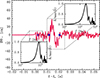 |
Fig. B.1. GW evolution during the first 55 ms for model s0.6-1. The blue cross marks the end of the bounce peak, and the blue circles locate the beginning and end of post-bounce oscillation. Insets show the normalised Fourier transform of the strain, |

Appendix C: Detectability of computed events
Due to their complex nature, GWs from CCSNe encode a significant amount of information. However, because of their weak intensity, a relatively nearby galactic event is necessary to capture most of this information. To infer the detectability of GWs, we employ the pipeline pnsInf (Bruel et al. 2023), which is designed to infer the properties of a PNS from its waveform. We assess the detectability of two main quantities: (i) the time of bounce and (ii) the ratio  of the PNS. Since the sky coverage of the detectors changes throughout the day due to Earth’s rotation, we quantify how favourable the arrival time of an event is. We use the equivalent antenna pattern weighted by the nominal reach of each detector:
 (C.1)
(C.1)
where F+k and F×k are the detector response functions, Ω is the position of the source in the sky (relative to an Earth-fixed coordinate system), t0 is the GPS time of arrival (at the centre of the Earth), and wk represents the nominal reach of each detector.
Considering that most stars are located in the bulk of the Milky Way, we account for the sky coordinates and times of arrival for the best (worst) case scenario in the bulk direction (here taken as an ellipse centred at the galaxy centre of semi-minor and major axes of 15° and 20°, respectively) where Feq is maximum (minimum). From now on, we refer to the ‘best case’ as the event with sky coordinates RA 16.99 h and Dec −35.59° and time of arrival 1393213818 s, and the ‘worst case’ as the one with RA 17.48 h, Dec −13.99° at 1393238418 s.
Prior to using the pipeline, we pad our waveforms with zeros before the bounce time and after the end of the simulation to avoid any boundary effects when calculating the time-frequency maps. Assuming a certain distance of the source from the detector network, we injected the waveforms into random Gaussian noise, which was different for every source and distance, and therefore modified the signal-to-noise of each event.
For the recovery of the time of bounce, we calculate the time-frequency maps for each detector in the network with a time window of 10 ms. We then search for the brightest column of pixels in each detector in the frequency band 100–1100 Hz, which are the typical frequencies present during the bounce. We consider the process successful if the recovered time lies within a 15 ms window of the actual time of bounce.
To infer  using the pipeline, we inverted the relation found in Torres-Forné et al. (2019a). We track the frequency of the likelihood calculated from the spectrograms computed with a 20 ms time window, starting from 25 ms after the bounce signal to avoid any signal arising from the bounce itself or strong prompt convection and PNS core ringdown oscillations happening in the few milliseconds after the bounce. Finally, we compare it with the real ratio derived from the simulation.
Detectability of the bounce signal for the full network of current generation detectors.
Percentage of the  ratio inferred with a network consisting of current generation Livingston and Hanford interferometers.
For both analyses, we employ a source distance ranging from 1 kpc to 200 kpc. While the bounce recovery is performed using the full interferometer network (LIGO, Virgo, and KAGRA), the mass-radius ratio inference uses just the two LIGO interferometers since they have the highest reach. The interferometer sensitivity is set to be the theoretical one for the O5 run (Abbott et al. 2020b).
In Tables C.1 and C.2, we show the detection results obtained from the LHVK network for inferring the bounce time and the  ratio, respectively. The bounce time can be well recovered until 30 kpc by at least one detector for almost every case and both scenarios. Additionally, in fast-rotating models or models in which resonance plays an important role, detection can be pushed up to 70 kpc for one detector, and for a subset of these latter ones to 100 kpc. However, as shown in Section 4.3, slow rotators do not present a strong bounce signal. Nonetheless, we can recover a bounce time very close to the actual one.
Appendix D: General properties of our simulations
 |
Fig. D.1. GW amplitude evolution of the 29 models presented in this work. The red and blue portions of the amplitude correspond to the bounce and prompt convection signal, respectively. |
In this section, we collect data related to our simulation sample. Table D.1 lists the quantitative results from our analysis and Figure D.1 shows the waveforms of the models presented in this study.
Quantitative results.
All Tables
Detectability of the bounce signal for the full network of current generation detectors.
Percentage of the ratio inferred with a network consisting of current generation Livingston and Hanford interferometers.
All Figures
|
Fig. 1. Evolution of GW amplitude for models s0.0-1 (A), s1.0-1 (B), and s2.0-1 (C). Panels from top to bottom show the time evolution of the GW amplitude for the whole simulation domain, PNS core, sonic envelope, and outer layers. Finally, the bottom row shows the space-time evolution of 𝒟h(t, r). Dashed, solid, and dotted lines represent the PNS core, sonic envelope, and PNS average radius, respectively. Grey shades mark regions where N2 < 0, i.e. approximately, regions where convection takes place. Numbered ellipses identify GW modes in each region (see text). |
| In the text | |
|
Fig. 2. Time evolution of the total GW strain and the six sIMFs for model s1.2-1. The dashed blue line on the first panel represents the full strain extracted on the whole simulation domain, and the solid red line the strain as a sum of the sIMFs. |
| In the text | |
|
Fig. 3. Panels A and B show the difference between the highest and lowest points of the GW signal, Δh, against the rotational kinetic energy to gravitational energy ratio for bounce and post-bounce signals, and for PNS core (Δhcore) and convection (Δhconv) signals, respectively, for models with magnetic field configuration 1. Panels C and D display the frequencies of the previous intensity peaks in relation to the same quantity on the x axis for the same pool of models as in the previous two panels. |
| In the text | |
|
Fig. 4. Panel A: Snapshot of the entropy at 15 ms after bounce, showing the convective bubbles surrounding the PNS core. Panel B: Snapshot of the radial velocity at 65.7 ms, showing the propagation (here at 50 km) of a wave generated by oscillations of the PNS core and propagating outwards. Both snapshots are for model s1.0-1. |
| In the text | |
|
Fig. 5. GW amplitude (top row) and corresponding spectrograms for models s0.4-1 (panel A, representative of the class of slowly rotating models), s0.9-1 (B, prototype of intermediately rotating cases) and s2.4-1 (C, representative of the class of fast-rotating models), calculated with a time window of 10 ms. The red line corresponds to the convection frequency (Equation (8)) at the sonic envelope surface, the blue lines show the epicyclic frequency (solid) and its first overtone (dotted) in the π/4 direction at the PNS core surface, while the green line is the fundamental quadrupolar mode frequency (2f) computed with the quasi-universal relation in Torres-Forné et al. (2019b). |
| In the text | |
|
Fig. 6. Evolution of the frequency of the convection strain expressed as the IF of the sum of the last three sIMFs (blue line) and as the frequency associated with the convective velocity for model s0.4-1. |
| In the text | |
|
Fig. 7. Evolution of the first 100 ms of the total rotational kinetic energy of PNS core and sonic envelope divided by the total gravitational energy for the four magnetic field configurations of model s1.0. |
| In the text | |
|
Fig. 8. Same as Figure 5 but for models s0.6-4, s1.0-4, and s1.8-4. The residual was removed to prevent the low-frequency memory signal from masking the convection signal. |
| In the text | |
|
Fig. 9. Time-frequency diagrams of the GW strain at 10 kpc injected into Gaussian noise for models s0.2-1 (panel A), s0.9-1 (panel B) and s1.8-1 (panel C), as seen by the LIGO Livingston interferometer for an event occurring at RA 16.99 h, Dec −35.59° and arrival time 1393213818 s. |
| In the text | |
|
Fig. B.1. GW evolution during the first 55 ms for model s0.6-1. The blue cross marks the end of the bounce peak, and the blue circles locate the beginning and end of post-bounce oscillation. Insets show the normalised Fourier transform of the strain, |
| In the text | |
|
Fig. D.1. GW amplitude evolution of the 29 models presented in this work. The red and blue portions of the amplitude correspond to the bounce and prompt convection signal, respectively. |
| In the text | |
Current usage metrics show cumulative count of Article Views (full-text article views including HTML views, PDF and ePub downloads, according to the available data) and Abstracts Views on Vision4Press platform.
Data correspond to usage on the plateform after 2015. The current usage metrics is available 48-96 hours after online publication and is updated daily on week days.
Initial download of the metrics may take a while.