| Issue |
A&A
Volume 705, January 2026
|
|
|---|---|---|
| Article Number | A2 | |
| Number of page(s) | 14 | |
| Section | Galactic structure, stellar clusters and populations | |
| DOI | https://doi.org/10.1051/0004-6361/202556545 | |
| Published online | 23 December 2025 | |
Tracing ωCentauri’s origins: Spatial and chemical signatures of its formation history
1
Istituto Nazionale di Astrofisica – Osservatorio Astronomico di Padova,
Vicolo dell’Osservatorio 5,
Padova
35122,
Italy
2
Dipartimento di Fisica e Astronomia “Galileo Galilei”, Univ. di Padova,
Vicolo dell’Osservatorio 3,
Padova
35122,
Italy
3
Dipartimento di Tecnica e Gestione dei Sistemi Industriali, Università degli Studi di Padova,
Stradella S. Nicola 3,
36100
Vicenza,
Italy
4
South-Western Institute for Astronomy Research, Yunnan University,
Kunming
650500,
PR
China
★ Corresponding author: This email address is being protected from spambots. You need JavaScript enabled to view it.
Received:
22
July
2025
Accepted:
20
September
2025
Abstract
ωCentauri (ωCen), with its unmatched chemical complexity, is the most enigmatic Galactic globular cluster (GC). We combine photometric and spectroscopic catalogs to identify distinct stellar populations within ωCen, investigate their spatial distribution and chemical properties, and uncover new insights into the cluster’s formation history. Our population tagging identified the iron-poor stars commonly found in most GCs: the first population (1P), with halo-like chemical composition, and the second population (2P), enriched in elements produced by proton-capture processes. Similarly, we divided the iron-rich stars (the anomalous stars) into two groups, AI and AII, which exhibit light-element abundance distributions similar to 1P and 2P stars, respectively. The wide radial extension of our dataset (five times the half-light radius) allowed us, for the first time, to directly and unambiguously compare the fractions of these populations at different radii. We find that the 2P and AII stars are more centrally concentrated than the 1P and AI stars. The remarkable similarities between the 1P-2P and AI-AII radial distributions strongly suggest that these two groups of stars originated through similar mechanisms. Our chemical analysis indicates that the 1P and AI stars (the lower stream) developed their inhomogeneities through self-enrichment from core-collapse supernovae (and possibly ejecta from other massive stars), as supported by their increasing α-element abundances with [Fe/H]. These populations contributed proton-capture-processed material to the intracluster medium, from which the chemically extreme 2P and AII stars (the upper stream) formed. Additional polluters, such as intermediate-mass asymptotic giant branch stars and Type Ia supernovae, likely played a role in shaping the AII population. Finally, we propose that 2P and AII stars with intermediate light-element abundances (the middle stream) formed via dilution between the pure ejecta that created the upper stream and the lower-stream material.
Key words: stars: abundances / stars: chemically peculiar / stars: Population II
© The Authors 2025
 Open Access article, published by EDP Sciences, under the terms of the Creative Commons Attribution License (https://creativecommons.org/licenses/by/4.0), which permits unrestricted use, distribution, and reproduction in any medium, provided the original work is properly cited.
This article is published in open access under the Subscribe to Open model. This email address is being protected from spambots. You need JavaScript enabled to view it. to support open access publication.
1 Introduction
Decades of research have revealed that most massive old Galactic globular clusters (GCs) exhibit star-to-star chemical inhomogeneities, particularly in light elements, leading to well-known C–N, O–Na, and Mg–Al abundance anticorrelations (e.g., Marino et al. 2008; Carretta et al. 2009; Mészáros et al. 2020). These patterns arise because, in addition to stars with halo-like chemical compositions, referred to as first-population (1P) stars, GCs host second-population (2P) stars enriched in He, N, Na, and Al, and depleted in C, O, and Mg (see reviews by Bastian & Lardo 2018; Gratton et al. 2019; Milone & Marino 2022).
The picture is complicated by the presence of further stellar populations in one-fifth of the studied Galactic GCs (typically referred to as “anomalous” in contrast to the “canonical” 1P and 2P stars), which are enriched in total C+N+O, [Fe/H], and/or s-process elements. These constitute the so-called Type II GCs, whereas Type I clusters lack such stars (e.g., Marino et al. 2009; Yong et al. 2015; Milone et al. 2017; Dondoglio et al. 2023). While different scenarios have been proposed to explain the chemical profiles of these objects, such as prolonged star formation (e.g., D’Antona et al. 2016) and the merging of different GCs (e.g., Bekki & Tsujimoto 2016; Mastrobuono-Battisti et al. 2019; Calamida et al. 2020), their origin remains uncertain.
Among the already exceptional Type II GCs, ωCentauri (ωCen) stands out as the most complex and peculiar case. Numerous studies have revealed its extraordinary chemical diversity, including a broad [Fe/H] spread exceeding 1 dex with distinct peaks in its distribution (e.g., Norris & Da Costa 1995; Johnson & Pilachowski 2010; Nitschai et al. 2024), and multiple well-separated C–N, O–Na, and Mg–Al anticorrelations at different metallicities (e.g., Marino et al. 2011; Mészáros et al. 2021; Alvarez Garay et al. 2022). The amplitude of light-element variations in ωCen is among the largest observed in any GC, likely linked to its high mass, as such variations correlate with cluster mass (Milone et al. 2018; Mészáros et al. 2020; Dondoglio et al. 2025). Beyond iron and light elements, ωCen also shows strong s-process and total C+N+O enhancement, both of which increase with [Fe/H] and exceed the levels observed in any other Type II GC (Norris & Da Costa 1995; Smith et al. 2000; Johnson & Pilachowski 2010; Marino et al. 2011, 2012; Mészáros et al. 2021; Mason et al. 2025).
The remarkable chemical complexity of ωCen indicates the presence of numerous distinct populations. Photometric studies have revealed an increasing number of stellar sequences as the observational quality has improved. Early studies by Lee et al. (1999) and Bedin et al. (2004) identified split sequences in color-magnitude diagrams (CMDs) along the main sequence (MS), subgiant branch (SGB), and red giant branch (RGB). Bellini et al. (2017) used UV and optical Hubble Space Telescope (HST) data to detect at least 15 distinct populations in the MS. A major breakthrough came with the introduction of the chromosome map (ChM) – a pseudo-two-color diagram constructed from the F275W, F336W, F438W, and F814W HST filters (Milone et al. 2015) – which enabled unprecedented population tagging. Using the ChM, Milone et al. (2017) identified 1P, 2P, and anomalous RGB stars in the central 2 arcmin of ωCen. More recently, Häberle et al. (2024) extended this capability to ~5 arcmin, expanding the radial coverage for ChM-based population tagging.
Radially extended population tagging is instrumental in deriving spatial distributions, an essential aspect of GC studies, as the observed population gradients (e.g., Milone et al. 2012b; Lee 2017; Leitinger et al. 2023) are closely tied to both formation mechanisms and dynamical evolution (Mastrobuono-Battisti & Perets 2016; Dalessandro et al. 2019; Vesperini et al. 2021). Previous studies traced the radial distribution of multiple distinct MSs (Sollima et al. 2007; Bellini et al. 2009; Scalco et al. 2024) to ~20 arcmin from the center, revealing that these populations are not fully mixed, with some more centrally concentrated than others. However, in a system as complex as ωCen, CMD-based MS separation does not allow an unambiguous assignment of these sequences to 1P, 2P, or anomalous populations, limiting comparison with spatial distributions in other GCs.
The origin of ωCen’s complex structure has long been debated. A widely accepted scenario suggests that ωCen is the remnant nucleus of a more massive stellar system-likely a dwarf galaxy – whose outer regions were stripped during accretion by the Milky Way, as first modeled by Bekki & Freeman (2003). Supporting this view, Pagnini et al. (2025) pointed out that other GCs show chemical similarities with ωCen, implying a common origin within the same progenitor galaxy. The idea of ωCen being a nuclear star cluster of this progenitor galaxy has been frequently considered, with the cluster resulting from a mixture of in situ star formation and infall of other GCs (Neumayer et al. 2020). In contrast, other studies suggested that the chemical complexity derived from self-enrichment due to a prolonged star formation, without invoking merger events (e.g., Pancino et al. 2007; Johnson & Pilachowski 2010).
Despite this, the detailed origin of its intricate light- and heavy-element abundance patterns remains uncertain. Alvarez Garay et al. (2024) identify a discontinuity in the Mg–Al trend, suggesting multiple formation channels for light-element inhomogeneities at different metallicities. Mason et al. (2025) propose that different groups of stars evolved separately in a GC-like environment and later merged to assemble ωCen. In contrast, Marino et al. (2012) presented a scenario rooted in the self-enrichment framework previously proposed for all GCs (e.g., Prantzos & Charbonnel 2006), but extended to account for the complexity of this particular system. In this scenario, 1P-like stars formed first, followed by rapid starbursts that created heavy-element inhomogeneities, leading to the formation of subsequent generations with light-element variations via self-pollution. Another ongoing debate, closely tied to its formation history, concerns the age spread of ωCen. Several studies based on CMD analyses of the SGB have suggested a total age range (from the youngest to the oldest population) up to ~2 Gyr (e.g., Lee et al. 1999; Villanova et al. 2014; Clontz et al. 2024). However, Tailo et al. (2016), using multiband HST data and stellar models, conclude that all stars likely formed within a much shorter period, not exceeding 0.5 Gyr. A key source of uncertainty in age determinations is the C+N+O variation, which can mimic age differences by producing similar SGB splits. Accurately constraining the total C+N+O content is therefore essential to resolving the age spread controversy.
In this work, we consistently identify 1P, 2P, and anomalous stars in ωCen from its center out to ~30 arcmin (approximately five times the half-light radius) for the first time, using multiple photometric and spectroscopic datasets to investigate their spatial distribution and chemical composition. Section 2 describes the datasets used in this study. In Section 3, we apply these data to identify the same populations across different datasets over a wide radial range. Section 4 examines the radial distribution of the identified populations. Section 5 explores the chemical composition of the different stellar components, while Section 6 presents our reconstruction of the formation sequence that shaped the cluster. Finally, our main results and conclusions are summarized in Section 7.
2 Dataset
We combined photometric and spectroscopic datasets of ωCen to identify distinct stellar populations along the RGB across a wide range of radial distances from the cluster center.
We utilized three photometric catalogs in our analysis. First, we used the dataset and ChM published by Milone et al. (2017), constructed from UV and optical HST photometry in the F275W, F336W, F438W, and F814W filters, which cover the innermost ~2 arcmin of the cluster. Second, we used the HST catalog by Häberle et al. (2024), which includes multi-epoch HST and optical photometry in bands suitable for constructing a ChM. This catalog combines decades of observations across different fields of view, extending up to ~5 arcmin from the center. The photometry was corrected for differential reddening following the procedure described by Milone et al. (2012a). Third, we incorporated Gaia photometry (Gaia Collaboration 2023) to assess membership for stars located beyond the 5 arcmin radius not included in the previous two HST-based catalogs. We selected ωCen members based on high-quality Gaia photometry1, proper motions, and parallaxes consistent with GC stars, following the approach of Cordoni et al. (2018) and Jang et al. (2022).
Our primary spectroscopic dataset is drawn from the Apache Point Observatory Galactic Evolution Experiment (APOGEE) Data Release 17 (DR17; Abdurro’uf et al. 2022), from which we selected only bright stars with signal-to-noise ratios >70 and excluded sources flagged with ASCAPFLAG = STAR_BAD2. For a comprehensive overview of our selection criteria, we refer the reader to Dondoglio et al. (2025). We considered the following abundance ratios from APOGEE: [C/Fe], [N/Fe], [O/Fe], [Mg/Fe], [Al/Fe], [Si/Fe], [Ca/Fe], [Fe/H], and [Ce/Fe]. Additionally, we included two other datasets, using measurements of [Na/Fe], [Ba/Fe], and [La/Fe] from Marino et al. (2011) and A(Li) abundances from Mucciarelli et al. (2018). Across all spectroscopic datasets, we retained only stars that, according to photometric catalogs and radial velocities, are consistent with ωCen membership. This filtering also allowed us to exclude [C/Fe] and [N/Fe] measurements in stars brighter than the RGB bump, which are affected by extra mixing processes after the first dredge-up. These processes lead to carbon depletion and nitrogen enhancement depending on luminosity (e.g., Charbonnel et al. 1998; Shetrone et al. 2019; Lee 2023), potentially biasing our interpretation of chemical differences among cluster populations. Although lithium is similarly affected, we did not apply this additional selection to A(Li), as the dataset from Mucciarelli et al. (2018) already includes only stars located below the RGB bump. The spectroscopic dataset allowed us to derive abundances for ωCen stars out to about 30 arcmin from the cluster center.
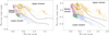 |
Fig. 1 Chromosome maps (ChMs) of the innermost two arcmin of ωCen published by (Milone et al. 2017) (left panel) and of the 2–5 arcmin region constructed from the HST catalog of Häberle et al. (2024) (right panel). The 1P, 2P, AI, and AII stars are shown in green, violet, blue, and orange, respectively. The two dot-dashed black lines separate the lower, middle, and upper streams in each panel. Black crosses mark stars that are present in our spectroscopic dataset presented in Section 2. |
3 Population tagging
In this section, we identify the different populations analyzed in this work, using multiple photometric and spectroscopic diagrams to identify them from the innermost area up to about 30 arcmin from the cluster center. Section 3.1 presents the ChMs constructed from HST photometry, while Section 3.2 describes how we tagged these populations using APOGEE spectroscopic data.
3.1 Populations in the chromosome map
The morphology of ωCen is more complex than that of any other GC. This is illustrated by the ΔCF275W,F336W,F438W versus ΔF275W,F814W ChM of RGB stars in the innermost ~2 arcmin published by Milone et al. (2017) and shown in the left panel of Figure 1. In this map, multiple populations form several distinct blobs of stars, as well as gaps and extended sequences. Consequently, classifying ωCen populations is challenging, and several classification models have been proposed over the years. Milone and collaborators divide the stars in the ChM into canonical stars, which form the 1P and 2P patterns typical of all GCs, and anomalous stars, which are characterized by iron, s-process, and C+N+O enhancements and are present in Type II GCs. Following the prescription of Milone et al. (2017), canonical stars form the bluest sequence on this diagram, with 1P stars forming a distinct clump around ΔF275W,F336W,F438W ~ 0 in the ChM, shown in green in Figure 1. The remaining sequence of stars, which span a ΔCF275W,F336W,F438W range between ~0.1 and 0.4, consists of 2P stars (in violet).
We then divided the anomalous stars into two subgroups using a similar approach: one population describes a sequence with low ΔCF275W,F336W,F438W (AI, blue), and the second includes all remaining anomalous stars (AII, orange). The position on the ChM suggests that AI does not exhibit nitrogen enhancement (primarily traced by the ChM y-axis), indicating that these stars did not form from material enriched by proton-capture (p-capture) processes. In contrast, the ChM position of AII stars suggests that they display signs of 2P-like chemical compositions, as also suggested by spectroscopy (e.g., Johnson & Pilachowski 2010; Marino et al. 2011; Alvarez Garay et al. 2024).
The right panel of Figure 1 shows the same population tagging on ΔCF275W,F336W,F435W versus ΔF275W,F814W ChM, obtained by applying the procedure of Milone et al. (2017, see their Appendix A) to RGB stars in the recent ωCen catalog published by Häberle et al. (2024). This catalog covers larger distances from the cluster center, allowing us to trace 1P, 2P, AI, and AII populations out to 5 arcmin. In both ChMs, black crosses mark the stars included in the spectroscopic dataset described in Section 2.
Another popular classification adopted in this work divides ωCen stars into three groups based on their position along the ChM y-axis: the lower, upper, and middle streams (Marino et al. 2019a; Clontz et al. 2024). The lower stream comprises all stars with no evidence of p-capture pollution, coinciding with 1P+AI, while the upper stream is composed of the most chemically extreme 2P and AII stars, characterized by the largest light-element inhomogeneities and the largest ChM y-axis coordinates. Finally, the middle stream consists of all 2P and AII stars located at intermediate ChM positions. The dot-dashed black lines in both panels of Figure 1 divide the three streams following the classification introduced by Marino et al. (2019a). Table 1 provides a summary of the different classification criteria and how they relate to each other.
Different classifications of ωCen populations (see text for details).
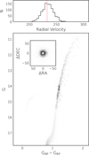 |
Fig. 2 Color–magnitude and radial-velocity diagrams of G vs. GBP-GRP from Gaia photometry. Gray points represent ωCen members with high-quality photometry, while black dots indicate the RGB stars with available APOGEE abundances, who reach up to ~30 arcmin radius. The inset shows the ΔDEC vs. ΔRA position respect to the cluster center (in arcmin) of the stars shown in the CMD. The top panel displays the radial velocity histogram of the selected sample of stars. |
3.2 APOGEE data in the outer regions
Beyond five arcmin, no ChMs are available to identify 1P, 2P, AI, and AII RGB stars. To overcome this limitation, we used an alternative approach that combined spectroscopic abundances from the APOGEE survey with Gaia photometry.
The first step consisted of assessing a sample of ωCen RGB stars located beyond a radius of five arcmin. To this end, we used the Gaia G versus GBP-GRP CMD of ωCen members (selected as described in Section 2), shown in Figure 2 for distances between five and 60 arcmin from the cluster center, as indicated in the inset panel. The stars marked with black dots represent RGB stars with available APOGEE abundances3. The top panel shows a histogram of the radial velocity values for our sample, which is distributed around the average radial velocity (pink line) reported by Baumgardt & Hilker (2018).
Our second step was to identify the counterparts of the 1P, 2P, AI, and AII populations. To achieve this, we used the [Al/Fe] versus [Fe/H] diagram of APOGEE abundances for all RGB stars from the center out to 30 arcmin, shown in panel a of Figure 3. This plot resembles the ChM in several respects, showing a continuous distribution of stars at [Fe/H]<−1.6 dex, populated by canonical stars, and two separated elongated sequences at higher iron content, corresponding to the upper and lower streams. The middle stream, with intermediate [Al/Fe], is almost absent at larger [Fe/H], consistent with what is observed in the ChM at larger ΔF275W,F814W. Panel b1 shows a zoomed-in view of the most metal-poor area, dominated by the canonical populations. Here, we colored all stars in the APOGEE catalog within five arcmin with available ChM population tagging. Unsurprisingly, the distinct blob at low [Al/Fe] (approximately −0.3 dex) is mostly populated by 1P stars and forms a separated peak in the [Al/Fe] kernel-density distribution portrayed in panel b2 (black line). We consider the stars with [Al/Fe] within the two horizontal dot-dashed green lines and [Fe/H] below than the brown vertical line in panel b1 as 1P stars. The vertical lines indicate the 90th percentile of the [Fe/H] distribution of stars within the Al peak. Guided by stars with known classification, we consider stars with [Al/Fe] between −0.05 and 1.10 dex and [FeH] below the brown-line level as 2P stars, since 2P stars are not iron-enriched compared to 1P stars. Panel b2 displays the [Al/Fe] kernel density distribution of 2P stars (violet line), revealing a distinct peak above [Al/Fe]~0.8 dex. We interpret this peak as the canonical part of the upper stream, i.e., the counterpart to the high-ΔCF275W,F336W,F438W 2P stars, which form a separate blob in the ChM. Panel c provides a zoom on the anomalous stars, showing that the elongated sequence below [Al/Fe] ~ 0.1 dex is populated by AI stars, while AII stars dominate the area above that level on the red side of the brown line, as expected from the ChM distribution.
Panel d presents the final result of our tagging, with stars in the [Al/Fe] versus [Fe/H] diagram beyond five arcmin colored according to their assigned population. As in Figure 1, the two dash-dotted black lines separate the lower, middle, and upper streams. Although the definition of the lower stream is straight-forward, as is the combination of 1P and AI stars, the separation of the middle and upper streams is not obvious along the entire diagram. We separated these visually based on the fact that the 2P stars above ~0.8 dex are likely to belong to the upper stream and that the middle stream tends to disappear at larger [Fe/H]. These observations, combined with spectroscopic evidence that the largest Al enhancements are expected among upper stream stars at each [Fe/H] (e.g., Marino et al. 2019a; Mason et al. 2025), ensured that our separation was generally reliable even in the [Al/Fe] versus [Fe/H] plane.
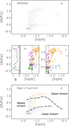 |
Fig. 3 Panel a: diagram of APOGEE [Al/Fe] vs. [Fe/H] for RGB stars in ωCen. Panel b1: zoom-in on the iron-poor end. Stars with ChM tagging are colored according to their assigned population, while the vertical dot-dashed line marks the 90th percentile of the 1P-star [Fe/H] distribution. Panel b2: normalized kernel-density distribution of [Al/Fe] for all stars (black) and for 2P stars (violet). The two dot-dashed horizontal green lines indicate the [Al/Fe] range of 1P stars. Panel c: same as panel b1 but zoomed on higher [Fe/H]. Panel d: [Al/Fe] vs. [Fe/H] For APOGEE stars located beyond 5 arcmin, colored according to the population tagging described in Section 3.2. The black lines mark the boundaries between the three streams, as reported in the plot. |
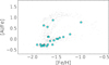 |
Fig. 4 [Al/Fe] vs. [Fe/H] diagram, as in Figure 3, with probable binaries highlighted by cyan diamonds. |
3.2.1 Binary stars
We also used the information present in the APOGEE dataset to identify candidate binary stars in our sample. To do this, we followed the approach outlined in the APOGEE documentation4 based on the VSCATTER quantity, which indicates the scatter of the radial velocity measured for each star in cases of multiple measurements. We identified stars as likely binaries using VSCATTER >1 kms−1, indicating a scatter much larger than observational errors, as recommended in the documentation.
Our sample contains 23 binaries that also have population tagging performed in Figure 3, all with three to thirteen radial velocity measurements. These are shown in Figure 4 as cyan diamonds in the [Al/Fe] versus [Fe/H] diagram. Of these, nine are 1P, three are 2P, eight are AI, and three are AII binaries. Most stars (about 70%) belong to the 1P and AI populations in this radial range (~5.9–21.6 arcmin). Notably, considering only the stars in the outer half of the sample (outside 14 arcmin), the incidence of 1P+AI binaries increases to about 90%.
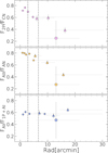 |
Fig. 5 Fraction of 2P stars relative to the total amount of canonical stars (top), AII stars relative to the bulk of anomalous (middle), and AI stars relative to the entire lower stream (bottom) plotted against the radial distance from the center of ωCen. Circles indicate fractions derived from the combined dataset, while triangles denote the APOGEE dataset only (see text for details). Diamonds represent fractions from binaries stars only. Gray lines show the radial intervals relative to each measurement, while the dot-dashed black lines mark the core and half-mass radii. |
3.2.2 Extended 1P sequence
A visual inspection of the [Al/Fe] versus [Fe/H] diagram in Figure 3 reveals that the 1P stars appear to be distributed over a more extended [Fe/H] range than the 2P stars. This is not unexpected, as small iron spread among 1P stars has been observed in an increasing number of GCs in recent years (e.g. Marino et al. 2019b; Legnardi et al. 2022; Marino et al. 2023; Dondoglio et al. 2025). We inferred the width of the iron spread among 1P stars following the procedure used by Dondoglio et al. (2025). Briefly, we calculated the difference between the 90th and 10th percentiles of the 1P [Fe/H] values and subtracted in quadrature the corresponding quantity measured from a simulated Gaussian distribution with sigma equal to the typical [Fe/H] observational error provided by the APOGEE dataset.
We find that the 1P width is 0.138±0.008, which is significantly larger than the 2P iron width (0.085±0.003). Moreover, we note that our measurement from direct spectroscopic information is in 1-σ agreement with the spread predicted by Legnardi et al. (2022) from the ChM distribution of 1P stars (0.148±0.011).
4 Spatial distribution
The population tagging described in Section 3 enabled an unprecedented analysis of the spatial distribution of RGB stars from different populations within ω Cen across a wide radial range.
In the upper panel of Figure 5, we present the radial distribution of the 2P star fraction with respect to the total number of canonical stars. Radial bins with equal numbers of stars are considered, first for the entire dataset (dots) and then for the outermost dataset only (triangles), as presented in Section 3.2, to increase the resolution in the less dense outer regions. The two vertical dot-dashed lines represent the core and half-mass radii from Baumgardt & Hilker (2018). The fraction of 2P stars decreases with distance from the center, nearly halving between the innermost and outermost regions (comparing values at the center and at 20 arcmin), indicating that 2P stars are more centrally concentrated than 1P stars. The diamond indicates the fraction of 2P binary stars, which is smaller than the one observed for the non-binary stars in the same radial interval, reaching around 0.25.
The central panel displays similar calculations but for the AII population compared with the bulk of anomalous. The AII stars are more centrally concentrated than the AI, mirroring the pattern seen between 2P and 1P stars. Moreover, the radial distributions of 2P and AII (and, consequently, of 1P and AI) stars span similar ranges, with values decreasing from approximately 0.75 in the innermost 3 arcmin to 0.40 beyond 10 arcmin. A further similarity is seen in the AII binary fraction, which is smaller than the AII non-binary fraction over a similar radial range.
The lower panel shows the fraction of AI stars relative to the total number of 1P and AI stars (i.e., the bulk of the lower stream). This ratio remains relatively constant (~0.6) over the 30 arcmin range, with no obvious differences from the binary fraction.
We tested the statistical significance of the observed radial trends using a Kolmogorov-Smirnov test to obtain a p-value, which measures the likelihood that the observed distributions result from random statistical fluctuations rather than intrinsic variations. The distributions in the upper and middle panels of Figure 5 have p-values below 0.01, supporting the hypothesis that the observed radial variations are physical. In contrast, the fraction of AI stars relative to 1P stars has a p-value of 0.60, strongly suggesting that the flat distribution is intrinsic. Overall, the p-value test confirms the trends visually inspected in this section.
This is the most comprehensive and unequivocal identification of 1P and 2P stars over such a wide radial range in ωCen, providing a robust confirmation of previous results on 2P star segregation (e.g., Sollima et al. 2007; Bellini et al. 2009; Johnson & Pilachowski 2010; Scalco et al. 2024). The higher fraction of 1P binaries supports this idea: since 2P stars formed in a more centrally concentrated environment, their disruption rate is higher than that of the more diffused 1P stars (e.g., Vesperini et al. 2011; Hypki et al. 2022), leading to a smaller number of 2P binaries, as also observed in other GCs (e.g., D’Orazi et al. 2010; Lucatello et al. 2015; Dalessandro et al. 2018; Bortolan et al. 2025). Interestingly, AI and AII stars exhibit both radial distributions and binary incidence similar to those of 1P and 2P stars, respectively. This strongly suggests that the 2P and AII populations formed through similar mechanisms after the 1P and AI stars had already developed.
5 Exploring the chemical composition of ωCen
Our finding in Section 4 that the 1P and AI populations, and the 2P and AII populations, have similar spatial distributions suggests that these two pairs of populations share a common formation origin. To further explore this idea, this section explores the chemical composition of the different populations identified in ωCen, with a particular focus on the three streams. Section 5.1 compares the chemical composition of the lower and upper streams, while Section 5.2 focuses on the middle stream.
5.1 Comparing the lower and upper streams
In Figure 6, we examine the distributions of light-element abundances as a function of [Fe/H] for stars in the lower and upper streams. The considered abundances – A(Li), [C/Fe], [N/Fe], [O/Fe], [Na/Fe], [Mg/Fe], [Al/Fe], and [Si/Fe] – are all known to differ between the two streams (e.g., Johnson & Pilachowski 2010; Marino et al. 2011; Mucciarelli et al. 2018; Marino et al. 2019a; Alvarez Garay et al. 2024; Mason et al. 2025). Stars are color-coded according to their association with the 1P, 2P, AI, and AII populations. Upper stream stars, on average, exhibit lower abundances of Li, C, O, and Mg, and higher abundances of N, Na, and Al. These differences are broadly consistent with the upper stream having formed from a material polluted by the ejecta of high-mass stars belonging to the lower-stream population.
However, intrinsic abundance variations with [Fe/H] complicate the interpretation of these trends. To test for potential correlations, we calculated the Spearman’s rank correlation coefficient (Rs), reported in each panel. The associated uncertainties were derived from the standard deviation of 1,000 resamplings, with data points scattered according to their observational errors. In the lower stream, [C/Fe], [O/Fe], [Mg/Fe], [Al/Fe], and [Si/Fe] show positive correlations with [Fe/H], whereas A(Li), [N/Fe], and [Na/Fe] appear roughly constant. The upper stream displays both similarities and key differences: A(Li), [O/Fe], and [Mg/Fe] follow trends comparable to those of the lower stream, but other elements diverge. In particular, [C/Fe] remains constant, while [Na/Fe] and [N/Fe] increase sharply with [Fe/H]. The [Al/Fe] trend in the upper stream describes an arc-like structure, peaking around [Fe/H]~−1.6 dex before declining at higher metallicities. Notably, [Si/Fe] in the upper stream anticorrelates with [Fe/H], opposite to the trend observed in panel h1. Consequently, Si is higher than in the lower stream only at low metallicity, with this trend reversing at higher [Fe/H].
The increase in [O/Fe], [Mg/Fe], and [Si/Fe] among lower stream stars points toward an overall enhancement of α-elements with increasing [Fe/H]. To further investigate this, we calculated the mean [α/Fe] for lower stream stars by averaging their [O/Fe], [Mg/Fe], [Si/Fe], and [Ca/Fe] abundances. The upper panel of Figure 7 shows the [Ca/Fe] versus [Fe/H] trend for the lower stream. For completeness, we also present the same plot for the upper stream in the middle panel. The lower panel displays the resulting [α/Fe] for the lower stream, which, as expected, increases with iron content.
Finally, we turn our attention to the s-process elements and the total [C+N+O/Fe], which are known to vary significantly in ωCen (e.g., Marino et al. 2011; Mészáros et al. 2021). Figure 8 presents the behavior of the lower and upper streams for the available s-process element measurements, including [Ce/Fe] from APOGEE (panels a1 and a2) and the average of [Ba/Fe] and [La/Fe] ([⟨Ba, La⟩/Fe], panels b1 and b2) from Marino et al. (2011). The [Ce/Fe] abundance clearly increases with [Fe/H], as confirmed by the corresponding Rs values. A similar trend is evident in the barium and lanthanum average, albeit derived from a smaller sample. Interestingly, at low metallicity, the two streams exhibit similar s-process abundances, but at higher [Fe/H], the upper stream shows higher [Ce/Fe], as first reported by Mason et al. (2025).
The comparison between the lower and upper streams underscores the complexity of interpreting their origins. Although a scenario in which the lower stream formed first and enriched the intracluster medium – leading to the formation of the upper stream – is consistent with the observed chemical differences, it cannot fully explain the morphologies presented in Figures 6, 7 and 8. We explore this issue in more depth in Section 6.
 |
Fig. 6 elemental abundances A(Li), [C/Fe], [N/Fe], [O/Fe], [Na/Fe], [Mg/Fe], [Al/Fe], and [Si/Fe] vs [Fe/H] for lower-stream (panels a1-h1) and upper-stream (panels a2-h2) stars. Green, purple, violet, and orange dots represent 1P, AI, 2P, and AII stars, respectively. The numbers reported in the panel indicate the Spearman’s correlation coefficient and its associated uncertainty. |
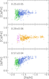 |
Fig. 7 Same as Figure 6 but for [Ca/Fe] of lower- and upper-stream stars (upper and middle panel, respectively), and [α/Fe] vs. [Fe/H] for 1P and AI stars (lower panel). |
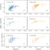 |
Fig. 8 Same as Figure 6 but for [Ce/Fe] (upper panels), [⟨Ba, La⟩/Fe] (middle panels), and [(C+N+O)/Fe] (lower panels) vs. [Fe/H] for lower- and upper-stream stars. |
5.2 The intermediate nature of the middle stream
The middle stream comprises 2P and AII stars whose positions along the ChM y-axis and [Al/Fe] values lie between those of the upper and lower streams. Its most distinctive feature is a narrower [Fe/H] distribution compared to the other two streams. It is more commonly found among canonical stars but becomes increasingly rare at higher [Fe/H] (and ChM x-axis) values.
Figure 9 illustrates the intermediate chemical behavior of the middle stream, showing median values for 2P and AII stars in violet and orange, respectively, for A(Li), [C/Fe], [N/Fe], [O/Fe], [Na/Fe], [Mg/Fe], [Al/Fe], [Si/Fe], [Ca/Fe], [Ce/Fe], [⟨Ba, La⟩/Fe], and [(C+N+O)/Fe]. The associated error bars indicate the standard deviation of the measurements. For comparison, solid and dashed gray lines show the second-order polynomial best fits to the lower and upper streams, respectively. The detailed abundance distributions for all considered elements, analogous to Figures 6 and 8, are presented in Appendix B. Both the 2P and AII middle stream components lie between the two gray lines for elements from Li to Al, while for [Si/Fe] both populations exhibit values similar to the lower stream. No significant differences in calcium are observed between the three streams. Within the limited [Fe/H] range covered by these stars, we do not detect significant differences between the median values of 2P and AII stars, suggesting no strong increasing or decreasing trends with [Fe/H]. A possible exception is [Na/Fe], for which the AII population shows a higher median value compared to 2P stars, although the two are consistent within 1σ. The RS values (in Appendix B) confirm that [Na/Fe] is the only light element showing a correlation with [Fe/H] (Rs = 0.54 ± 0.12).
In the last three panels of Figure 9, we present the same analysis for the s-process elements [Ce/Fe], [⟨Ba, La⟩/Fe], and the total [(C+N+O)/Fe]. In all three cases, the average values for the middle stream tend to lie closer to those of the lower stream. However, the large dispersion prevents definitive conclusions. Nonetheless, the median values suggest potential increasing trends with [Fe/H], which are supported by their respective Spearman’s correlation coefficients (see Appendix B).
 |
Fig. 9 Median A(Li), [C/Fe], [N/Fe], [O/Fe], [Na/Fe], [Mg/Fe], [Al/Fe], [Si/Fe], [Ca/Fe], [Ce/Fe], [⟨Ba, La⟩/Fe], and [(C+N+O)/Fe] vs. [Fe/H] of 2P (violet) and AII (orange) middle-stream stars. The continuous and dashed gray lines mark the average trends of the lower and upper streams, respectively. |
6 The formation history of ωCen
In this section, we gather the observational evidence presented throughout this work to reconstruct the sequence of events that led to the fascinating complexity of ωCen. Sections 6.1, 6.2 and 6.3 explore the possible origins of the lower, upper, and middle streams, respectively, while Section 6.4 summarizes the formation history of ωCen.
6.1 The lower stream
The 1P stars were likely the first generation to form in ωCen, originating directly from its primordial gas cloud. In nearly all proposed scenarios for multiple stellar populations, the 1P stars precede the 2P stars. The lower metallicity of 1P stars compared to the anomalous populations (see also Figure 19 from Johnson & Pilachowski 2010) strongly supports their earlier formation, as continued star formation typically leads to progressive iron enrichment.
A promising scenario for AI star formation involves self-enrichment via core-collapse supernovae (CCSNe), originally proposed by Marino et al. (2012) and recently supported by Mason et al. (2025). The CCSNe produce α-elements more efficiently than iron (e.g., Woosley & Weaver 1995; Nomoto et al. 2006; Marassi et al. 2019; Boccioli & Roberti 2024), potentially explaining the observed rise in [α/Fe] with [Fe/H] in the lower stream (see Figure 7). In this context, AI stars may have formed shortly after the 1P stars, from gas enriched by CCSN ejecta.
Figure 10 compares the predicted CCSN yields from a simple stellar population (SSP) with the observed lower stream trends for [C/Fe], [N/Fe], [O/Fe], [Na/Fe], [Mg/Fe], [Al/Fe], [Si/Fe], [Ca/Fe], and [Ce/Fe] as functions of [Fe/H]. The yields were generated using the one-zone chemical evolution code Chempy (Rybizki et al. 2017), simulating CCSN enrichment from a 108 M⊙ SSP with initial abundances matching 1P stars (open black dots) and assuming a Kroupa (2001) initial mass function. The simulation spans 40 Myr, corresponding to the typical timescale of CCSN activity. We emphasize that this comparison is qualitative and illustrative; a detailed model-to-data fit is beyond the scope of this study. Our goal was to evaluate whether CCSN yields align with the observed abundance trends.
The cumulative yields at 40 Myr are shown as a blue square and a red triangle, representing two CCSN yield sets: Limongi & Chieffi (2018, LC2018) and Nomoto et al. (2013, N2013), respectively. Both predict rising [Fe/H], [O/Fe], and [Si/Fe], consistent with observations. The N2013 yields reproduce the [Mg/Fe], [Al/Fe], and [Ca/Fe] trends, whereas LC2018 alone predicts a positive [C/Fe] trend – although much smaller than observed. The models also diverge significantly in [N/Fe]: LC2018 reproduces the observed flat trend, whereas N2013 shows a decline inconsistent with the data. Minor discrepancies are also seen in [Na/Fe]. These differences likely arise from the adopted stellar mass ranges: N 2013 includes stars from 13 to 40 M⊙, while LC2018 extends to 13–120 M⊙. For [Ce/Fe] – available only from LC2018 – the predicted increase is modest and does not explain the observed substantial enrichment.
While the models do not match all abundance trends, they exhibit encouraging qualitative agreement, particularly for key α-elements such as oxygen, Mg, Si, and Ca. These results support the idea that CCSNe played a major role in shaping the chemical evolution of the lower stream, making it a viable and promising formation scenario. However, substantial mismatches remain, especially for carbon and cerium, highlighting the need for more detailed modeling and consideration of contributions from other sources beyond CCSNe. An intriguing possibility involves stellar rotation: simulations by Frischknecht et al. (2016) suggest that massive, rotating, metal-poor stars (15–40 M⊙) could yield substantial s-process enrichment and thus may explain the large increase in cerium. Nevertheless, the chemical composition of massive star yields is a debated topic, with several factors, such as the progenitor mass range, hypernova contributions, and pre-supernova yields, that heavily influence the chemical composition of subsequent stellar generations (see Kobayashi 2025, for a recent review).
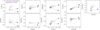 |
Fig. 10 Distribution of nine abundance ratios (see labels) vs. [Fe/H] for lower-stream stars, compared with CCSN yields from a simulated population, whose initial composition is indicated by the open black dots. The blue square and red triangle indicate yields derived from the tables of Limongi & Chieffi (2018) and Nomoto et al. (2013), respectively. |
6.2 The upper stream
The light-element chemical composition of the upper stream clearly indicates that these stars formed in a medium strongly polluted by the products of p-capture processes, exhibiting the characteristic depletion of Li, C, O, and Mg and enhancement of N, Na, and Al. In multiple-population formation scenarios, 2P stars with the most extreme chemical compositions are believed to be the first to form after the 1P stars, from the pure ejecta of polluters. Marino et al. (2012) proposed extending this idea to ωCen, with lower-stream stars at different [Fe/H] ejecting the material from which the upper stream originated, as a natural extension of the multiple-population theory. Our observation of AII stars showing similar radial segregation to 2P stars supports this idea, as this is a common feature of the multiple-population phenomenon.
In a simple model where the upper stream formed from the chemically processed ejecta of lower-stream stars, we would expect similar abundance trends with [Fe/H], simply shifted depending on the production or destruction of each element during the p-capture processes. However, Figure 6 shows a much more complex behavior. Moreover, the upper stream reaches [Fe/H] up to approximately −0.6 dex, but no lower-stream stars exhibit such a high value. These facts seem difficult to reconcile with the idea that the upper stream formed from lower-stream ejecta, but can be justified by considering additional physical processes.
First, the production of Mg, Al, and Si during the p-capture reactions is highly metallicity-dependent. At lower [Fe/H], higher core temperatures in polluter stars (>70 MK) ignite the Mg–Al cycle, depleting Mg and enhancing Al. At even higher temperatures (>100 MK), Si is produced through leakage from this cycle (Arnould et al. 1999; Prantzos et al. 2017). Thus, more metal-poor stars, being hotter, undergo stronger depletion of Mg depletion and enhancement of Al and Si, a pattern confirmed in several observations (e.g., Pancino et al. 2017; Dondoglio et al. 2025). This explains the steeper [Mg/Fe] decline with [Fe/H] seen in the upper stream, as Mg depletion decreases with increasing metallicity. The arc-shaped trend in [Al/Fe] follows a similar pattern. Between [Fe/H] ~ −1.7 and −1.4 dex, [Al/Fe] increases, echoing the behavior of its lower-stream progenitors. At higher [Fe/H], Al enhancement drops sharply, reversing the slope in the [Al/Fe]–[Fe/H] plane. The decline in [Si/Fe] in the upper stream shares the same physical origin: since Si production requires even higher temperatures than that of Al, its downturn begins at lower metallicities and thus lacks the initial upturn observed in Al. This metallicity dependence provides strong evidence that the p-capture processed material contributing to the formation of Fe-rich AII stars was ejected by stars that are more metal-rich than the 1P stars, with AI stars being the most likely candidates.
Second, additional sources of chemical enrichment may contribute. As increasingly metal-rich lower-stream stars pollute the medium, earlier generations (such as 1P stars) evolve and release ejecta from intermediate-mass AGB stars (3–4 M⊙) and from Type Ia supernovae. D’Antona et al. (2016) proposed these sources to explain the chemical anomalies in Type II GCs. Their material could mix with p-capture products and contribute to upper-stream formation, explaining the rise in [N/Fe] and [Na/Fe], both expected from AGB yields (Ventura et al. 2013; Karakas & Lattanzio 2014), and the higher [Fe/H] values in the upper stream, as Type Ia supernovae are prolific iron producers (e.g., Gronow et al. 2021; Keegans et al. 2023). In particular, 3–4 M⊙ AGB stars are believed to be major contributors to s-process elements (e.g., Karakas & Lattanzio 2014; Cristallo et al. 2015). If such stars influenced the formation of the upper stream, we would expect higher s-process abundances compared to those in the lower stream. This is supported by the [Ce/Fe] distributions in Figure 8, which show higher values in the high-[Fe/H] end of the upper stream.
Our observations agree with the idea that, similar to what is hypothesized for Type I GCs but extended to a structure with a longer star-formation history, the ejecta from the lower stream significantly contribute to the formation of upper-stream stars.
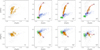 |
Fig. 11 Diagram of [Al/Fe] vs. [Fe/H] showing middle-stream AII stars highlighted by orange bullets (panel a). Panels a1, a2, and a3 present the same plot zoomed in around seq1, seq2, and seq3, respectively (see text), with lower-stream stars highlighted for reference. The best-fit fiducial lines are shown in red, with open and filled red symbols representing the 0% and 100% dilution points, respectively. Panels b, b1, b2, and b3, show the corresponding plots in the [Mg/Fe] vs. [Fe/H] plane. |
6.3 The middle stream
The middle stream offers arguably the most enigmatic chemical pattern of the three, with its much smaller [Fe/H] spread constituting one of the most challenging pieces to fit in solving the ωCen puzzle. The 2P stars in the middle stream offer a useful starting point for interpreting the origin of this stellar component. An extended 2P sequence with a wide range of light-element abundances is a common feature of massive Galactic GCs. A well-studied example is NGC 2808, which hosts a fraction of chemically extreme 2P stars, along with a more extended group of 2P stars whose compositions gradually resemble those of 1P stars (Carretta 2015; Milone et al. 2015; Carlos et al. 2023).
A popular explanation for this phenomenon involves a dilution mechanism (e.g., D’Antona et al. 2016; Carretta et al. 2018). In this scenario, the most extreme 2P stars form after the 1P stars from nearly pure ejecta in the dense central regions of a GC. Later, the intracluster medium – with 1P-like chemical composition – flows into the core and mixes with the residual ejecta, producing new 2P stars. As dilution increases, the resulting 2P stars increasingly resemble 1P stars in their chemical signatures. The intermediate chemical composition of middle stream 2P stars supports the dilution scenario, suggesting that these stars formed from a mixture of polluters’ ejecta and 1P-like material.
We also investigated whether dilution can explain the anomalous middle stream. In panel a of Figure 11, we highlight the AII stars associated with the middle stream (in orange) on the [Al/Fe] versus [Fe/H] diagram. They define three distinct sequences: Sequence 1 (seq1), from ([Fe/H], [Al/Fe])~(−1.65, 0.55) to (−1.55, 0.80), marked with squares in panel a1; Sequence 2 (seq2), from (−1.65, 0.05) to (−1.45, 0.80), shown with triangles in panel a2; and Sequence 3 (seq3), from (−1.55, 0.10) to (−1.10, 0.80), indicated by starred symbols in panel a3. In all three sequences, [Al/Fe] decreases as [Fe/H] decreases, a trend suggestive of dilution between material enriched in Al (from upper-stream stars) and a gas that is both Al- and Fe-poor. Analogous to Type I GCs, where 2P material is diluted by 1P-like gas, the most natural diluting agent here is gas resembling that of the lower stream.
To test this, we computed theoretical dilution curves. First, we selected upper-stream stars as the undiluted end members and converted their [Fe/H] and [Al/Fe] to mass fractions. Next, we mixed these with an increasing fraction of lower-stream-like material and calculated the resulting Fe and Al mass fractions. Finally, the diluted values were converted back to abundance ratios for comparison in the [Al/Fe] versus [Fe/H] plane. The dilution curves that qualitatively fit seq1, seq2, and seq3 are overplotted in red in panels a1, a2, and a3, respectively. In panels b, b1, b2, and b3, we repeated the analysis in the [Mg/Fe] vs. [Fe/H] plane to assess whether the derived dilution curves also align with the Mg trends of the middle-stream anomalous stars.
We find that seq1 is consistent with the dilution of upper-stream material with [Fe/H]~−1.40 by 1P-like gas (panel a1). The corresponding curve in the [Mg/Fe] versus [Fe/H] diagram (panel b1) also aligns with the observed data. Stars in seq1 span only part of the predicted dilution track, corresponding, in both [Al/Fe] and [Mg/Fe] distributions, to a dilution range of approximately 65–90%. For seq2, the starting point lies at a higher [Fe/H] (~−1.25 dex) and the dilution agent must be more metalrich than typical 1P gas ([Fe/H]~−1.60). Dilution with 1P-like gas fails to reproduce the observed trends, particularly in the [Mg/Fe] versus [Fe/H] diagram (panel b2), where the sequence clearly moves toward the AI region of the diagram. As in seq1, data in both plots span a similar dilution range (~55–100%). Finally, seq3 shows an inconsistency between its Al and Mg trends. While both panels a3 and b3 indicate dilution with lower-stream gas of [Fe/H]~−1.55, the initial (0% dilution) point that fits the Al trend ([Fe/H]~−0.95) does not match the Mg trend, which requires an iron-richer end by ~0.20 dex.
Our qualitative analysis indicates that dilution is a viable explanation for the middle stream, at least for two of the three identified sequences. The corresponding requirement for an increasingly iron-rich diluting agent to reproduce sequences with higher [Fe/H] supports our hypothesis (Section 6.3) that the iron-rich upper-stream stars formed in an environment progressively enriched in iron – likely by stars along the AI sequence.
6.4 Putting the pieces together
Based on the observational results presented in Sections 3–5 and the discussion in Sections 6.1–6.3, we propose a possible star formation sequence that led to ωCen.
The 1P stars formed first from the primordial molecular cloud. Unlike typical GCs, ωCen’s deep potential well retained CCSNe ejecta, enabling the formation of AI stars from increasingly enriched gas – likely facilitated by its early role as part of a more massive system, such as a dwarf galaxy. Later, 1P massive stars (depending on the nature of the multiple populations polluter) polluted the central regions with material enriched in p-capture elements, forming from pure ejecta upper stream 2P stars. As 1P-like gas flowed inward, it diluted this ejecta, producing 2P stars with compositions closer to the 1P population (see D’Antona et al. 2016). The radial distribution of these stars (Figure 5) preserves this evolutionary imprint. A similar process occurred for AI stars, which evolved later. Their ejecta formed the upper stream AII population, progressively enriched in Fe and α-elements, but also affected by pollution from 1P AGB stars (~3–4 M⊙) and Type Ia SNe. These events increased Fe and s-process elements in upper stream stars (Figure 8). As with 2P stars, dilution with lower-stream-like gas occurred, reducing not only light-elements differences but also decreased the [Fe/H], since the diluting gas was Fe-poor compared to the newly forming stars. Table C.1 summarizes the formation timeline, chemical features, and proposed origins of these populations.
The timescale at which this whole formation history might occur (i.e., the age spread of ωCen) depends on several assumptions regarding the different polluters involved, such as the mass range of exploding stars in the CCSNe phase, the Type Ia supernovae rate in a ωCen like environment, and the AGB nucleosynthesis assumptions in different mass ranges. An in-depth modeling of these phenomena is beyond the scope of the current work, which focuses on providing observational constrains. However, we point out, based on the scheme proposed by D’Antona et al. (2016, see their table 4), that the CCSNe phase should end ~40 Myr after the formation of the 1P, while the intermediate-mass AGB and Type Ia supernovae are expected to start polluting the medium after ~100 My. Moreover, after enough time (~300–400 Myr, Ventura et al. 2013) also the ejecta from lower-mass AGB stars (<3 M⊙) start pollute the cluster medium. These stars mostly produce a carbon enrichment, which is only observed in the lower stream. However, pollution from these sources cannot increase heavier elements such as magnesium, aluminum and sodium (Ventura et al. 2022, and references therein), thus with CCSNe ejecta being a much more realistic candidate for the formation of these stars. Consequently, the star formation history in ωCen would have ended before <3 M⊙ AGB stars strongly polluted the medium. These time scales suggest that the formation of ωCen lasted a few hundreds of Myr, in agreement with the estimate from Tailo et al. (2016), who posed 500 Myr as the maximum age spread, but at odds with other works in the literature, which derived a ~2 Gyr age difference between the youngest and oldest stellar populations (e.g., Villanova et al. 2014; Clontz et al. 2024).
7 Summary and conclusions
In our work, we combined multiple datasets to consistently track different ωCen populations from the cluster core out to ~30 arcmin, focusing on RGB stars. Our main findings are summarized below:
The combination of HST multi-band photometry and spectroscopic abundances enabled us to identify the canonical 1P and 2P, as well as the anomalous AI and AII populations, over an unprecedented radial extent – approximately five times the half-light radius. This approach ensures consistency between photometric and spectroscopic tagging.
This population tagging allowed us to investigate their radial distributions. We found that 2P stars are more centrally concentrated than 1P stars, as detected in other GCs. Moreover, the spatial distributions of the AI and AII populations mirror those of the 1P and 2P stars, respectively, with AII stars being more spatially concentrated than AI stars. Interestingly, binary stars are more prevalent among the 1P and AI populations, indicating a higher binary fraction compared to their chemically extreme counterparts.
Our dataset allowed a deep investigation of the chemical variety within the three streams and a their overall differences spanning the whole ωCen ’s [Fe/H] range. In particular, we provide robust constrain on the C+N+O content of each stream and their relation with metallicity, based-for the first time-only on stars below the RGB bump, thus not affected by mixing episodes.
A comparison between the lower stream (1P and AI stars) and the upper stream (chemically extreme 2P and AII stars) supports a scenario in which the upper stream formed from gas polluted by products of p-capture processes, synthesized and expelled into the intracluster medium by lower stream stars. However, to fully explain all the observed chemical features, additional polluting mechanism must be invoked.
Self enrichment from CCSNe ejecta constitutes the most promising mechanism behind the chemical inhomogeneities among lower stream stars. However, SSP yield models fail to reproduce the observed increases in certain abundance ratios-particularly for carbon and cerium- as [Fe/H] increases. Additional mechanisms, such stellar rotation in massive stars, may justify (at least) some of the discrepancies.
Starting from multiple-population scenarios that include dilution, we propose a similar mechanism to explain the chemical morphology of AII stars in the middle stream. In the [Al/Fe] vs. [Fe/H] diagram, three distinct sequences are evident, which we interpret as dilution curves between Al- and Fe-rich gas and the lower stream-like material, converging toward smaller [Fe/H] and [Al/Fe] values.
Based on the observational evidence gathered in our study, we propose a plausible sequence of events leading to the complex structure of ωCen. While the precise chronology depends on the origin of the proton-capture processed material and the timescales of the different polluters involved, the underlying scenario is the following: the lower stream stars pollute the intracluster medium with their ejecta, from which the upper stream stars subsequently form. Later, the middle stream emerges through the dilution of residual polluted gas (not collapsed into upper stream stars) with the intracluster material with chemical composition typical of lower stream stars. Notably, our scheme, based on spatial distribution and chemical composition only, is in overall agreement with kinematics investigations: upper stream stars exhibit significant radial anisotropy, while lower stream stars are nearly isotropic, a difference typically observed between the 1P and 2P of dynamically young GCs (Cordoni et al. 2020; Ziliotto et al. 2025), thus providing further, independent support that the whole upper and lower stream arose from a mechanism similar to the one producing 1P and 2P stars.
In this scenario, ωCen would form by self-enrichment processes, without the necessity of invoking merging events from several GCs. In this case, this cluster would constitute an extension of the so-called Type II GCs (where variation in iron, s-process elements and total C+N+O are observed) that originated from a more massive structure, likely a dwarf galaxy, allowing to retain a larger amount of massive stars ejecta and thus exhibiting a prolonged star formation history.
Data availability
Tables with Gaia ID, positions, and abundances of our spectroscopic sample are available at the CDS via https://cdsarc.cds.unistra.fr/viz-bin/cat/J/A+A/705/A2.
Acknowledgements
This work has been funded by the European Union – NextGenerationEU RRF M4C2 1.1 (PRIN 2022 2022MMEB9W: “Understanding the formation of globular clusters with their multiple stellar generations”, CUP C53D23001200006). T.Z. acknowledges funding from the European Union’s Horizon 2020 research and innovation programme under the Marie Skłodowska-Curie Grant Agreement No. 101034319 and from the European Union – NextGenerationEU".
References
- Abdurro’uf, Accetta, K., Aerts, C., et al. 2022, ApJS, 259, 35 [NASA ADS] [CrossRef] [Google Scholar]
- Alvarez Garay, D. A., Mucciarelli, A., Lardo, C., Bellazzini, M., & Merle, T. 2022, ApJ, 928, L11 [NASA ADS] [CrossRef] [Google Scholar]
- Alvarez Garay, D. A., Mucciarelli, A., Bellazzini, M., Lardo, C., & Ventura, P. 2024, A&A, 681, A54 [NASA ADS] [CrossRef] [EDP Sciences] [Google Scholar]
- Arnould, M., Goriely, S., & Jorissen, A. 1999, A&A, 347, 572 [NASA ADS] [Google Scholar]
- Bastian, N., & Lardo, C. 2018, ARA&A, 56, 83 [Google Scholar]
- Baumgardt, H., & Hilker, M. 2018, MNRAS, 478, 1520 [Google Scholar]
- Bedin, L. R., Piotto, G., Anderson, J., et al. 2004, ApJ, 605, L125 [Google Scholar]
- Bekki, K., & Freeman, K. C. 2003, MNRAS, 346, L11 [Google Scholar]
- Bekki, K., & Tsujimoto, T. 2016, ApJ, 831, 70 [NASA ADS] [CrossRef] [Google Scholar]
- Bellini, A., Piotto, G., Bedin, L. R., et al. 2009, A&A, 507, 1393 [NASA ADS] [CrossRef] [EDP Sciences] [Google Scholar]
- Bellini, A., Milone, A. P., Anderson, J., et al. 2017, ApJ, 844, 164 [NASA ADS] [CrossRef] [Google Scholar]
- Boccioli, L., & Roberti, L. 2024, Universe, 10, 148 [NASA ADS] [CrossRef] [Google Scholar]
- Bortolan, E., Bruce, J., Milone, A. P., et al. 2025, A&A, 696, A220 [NASA ADS] [CrossRef] [EDP Sciences] [Google Scholar]
- Calamida, A., Zocchi, A., Bono, G., et al. 2020, ApJ, 891, 167 [Google Scholar]
- Carlos, M., Marino, A. F., Milone, A. P., et al. 2023, MNRAS, 519, 1695 [Google Scholar]
- Carretta, E. 2015, ApJ, 810, 148 [Google Scholar]
- Carretta, E., Bragaglia, A., Gratton, R. G., et al. 2009, A&A, 505, 117 [NASA ADS] [CrossRef] [EDP Sciences] [Google Scholar]
- Carretta, E., Bragaglia, A., Lucatello, S., et al. 2018, A&A, 615, A17 [NASA ADS] [CrossRef] [EDP Sciences] [Google Scholar]
- Charbonnel, C., Brown, J. A., & Wallerstein, G. 1998, A&A, 332, 204 [NASA ADS] [Google Scholar]
- Clontz, C., Seth, A. C., Dotter, A., et al. 2024, ApJ, 977, 14 [Google Scholar]
- Cordoni, G., Milone, A. P., Marino, A. F., et al. 2018, ApJ, 869, 139 [CrossRef] [Google Scholar]
- Cordoni, G., Milone, A. P., Marino, A. F., et al. 2020, ApJ, 898, 147 [NASA ADS] [CrossRef] [Google Scholar]
- Cristallo, S., Straniero, O., Piersanti, L., & Gobrecht, D. 2015, ApJS, 219, 40 [Google Scholar]
- Dalessandro, E., Mucciarelli, A., Bellazzini, M., et al. 2018, ApJ, 864, 33 [NASA ADS] [CrossRef] [Google Scholar]
- Dalessandro, E., Cadelano, M., Vesperini, E., et al. 2019, ApJ, 884, L24 [Google Scholar]
- D’Antona, F., Vesperini, E., D’Ercole, A., et al. 2016, MNRAS, 458, 2122 [Google Scholar]
- Dondoglio, E., Milone, A. P., Marino, A. F., et al. 2023, MNRAS, 526, 2960 [Google Scholar]
- Dondoglio, E., Marino, A. F., Milone, A. P., et al. 2025, A&A, 697, A135 [NASA ADS] [CrossRef] [EDP Sciences] [Google Scholar]
- D’Orazi, V., Gratton, R., Lucatello, S., et al. 2010, ApJ, 719, L213 [CrossRef] [Google Scholar]
- Frischknecht, U., Hirschi, R., Pignatari, M., et al. 2016, MNRAS, 456, 1803 [Google Scholar]
- Gaia Collaboration (Vallenari, A., et al.) 2023, A&A, 674, A1 [NASA ADS] [CrossRef] [EDP Sciences] [Google Scholar]
- Gratton, R., Bragaglia, A., Carretta, E., et al. 2019, A&A Rev., 27, 8 [NASA ADS] [CrossRef] [Google Scholar]
- Gronow, S., Côté, B., Lach, F., et al. 2021, A&A, 656, A94 [NASA ADS] [CrossRef] [EDP Sciences] [Google Scholar]
- Gunn, J. E., Siegmund, W. A., Mannery, E. J., et al. 2006, AJ, 131, 2332 [NASA ADS] [CrossRef] [Google Scholar]
- Häberle, M., Neumayer, N., Bellini, A., et al. 2024, ApJ, 970, 192 [Google Scholar]
- Hypki, A., Giersz, M., Hong, J., et al. 2022, MNRAS, 517, 4768 [NASA ADS] [CrossRef] [Google Scholar]
- Jang, S., Milone, A. P., Legnardi, M. V., et al. 2022, MNRAS, 517, 5687 [CrossRef] [Google Scholar]
- Johnson, C. I., & Pilachowski, C. A. 2010, ApJ, 722, 1373 [NASA ADS] [CrossRef] [Google Scholar]
- Jönsson, H., Holtzman, J. A., Allende Prieto, C., et al. 2020, AJ, 160, 120 [Google Scholar]
- Karakas, A. I., & Lattanzio, J. C. 2014, PASA, 31, e030 [NASA ADS] [CrossRef] [Google Scholar]
- Keegans, J. D., Pignatari, M., Stancliffe, R. J., et al. 2023, ApJS, 268, 8 [NASA ADS] [CrossRef] [Google Scholar]
- Kobayashi, C. 2025, arXiv e-prints [arXiv:2506.20436] [Google Scholar]
- Kroupa, P. 2001, MNRAS, 322, 231 [NASA ADS] [CrossRef] [Google Scholar]
- Lee, J.-W. 2017, ApJ, 844, 77 [NASA ADS] [CrossRef] [Google Scholar]
- Lee, J.-W. 2023, ApJ, 950, L6 [Google Scholar]
- Lee, Y. W., Joo, J. M., Sohn, Y. J., et al. 1999, Nature, 402, 55 [Google Scholar]
- Legnardi, M. V., Milone, A. P., Armillotta, L., et al. 2022, MNRAS, 513, 735 [NASA ADS] [CrossRef] [Google Scholar]
- Leitinger, E., Baumgardt, H., Cabrera-Ziri, I., Hilker, M., & Pancino, E. 2023, MNRAS, 520, 1456 [NASA ADS] [CrossRef] [Google Scholar]
- Limongi, M., & Chieffi, A. 2018, ApJS, 237, 13 [NASA ADS] [CrossRef] [Google Scholar]
- Lindegren, L., Hernández, J., Bombrun, A., et al. 2018, A&A, 616, A2 [NASA ADS] [CrossRef] [EDP Sciences] [Google Scholar]
- Lucatello, S., Sollima, A., Gratton, R., et al. 2015, A&A, 584, A52 [NASA ADS] [CrossRef] [EDP Sciences] [Google Scholar]
- Marassi, S., Schneider, R., Limongi, M., et al. 2019, MNRAS, 484, 2587 [NASA ADS] [CrossRef] [Google Scholar]
- Marino, A. F., Villanova, S., Piotto, G., et al. 2008, A&A, 490, 625 [NASA ADS] [CrossRef] [EDP Sciences] [Google Scholar]
- Marino, A. F., Milone, A. P., Piotto, G., et al. 2009, A&A, 505, 1099 [CrossRef] [EDP Sciences] [Google Scholar]
- Marino, A. F., Milone, A. P., Piotto, G., et al. 2011, ApJ, 731, 64 [Google Scholar]
- Marino, A. F., Milone, A. P., Piotto, G., et al. 2012, ApJ, 746, 14 [CrossRef] [Google Scholar]
- Marino, A. F., Milone, A. P., Renzini, A., et al. 2019a, MNRAS, 487, 3815 [CrossRef] [Google Scholar]
- Marino, A. F., Milone, A. P., Sills, A., et al. 2019b, ApJ, 887, 91 [NASA ADS] [CrossRef] [Google Scholar]
- Marino, A. F., Milone, A. P., Dondoglio, E., et al. 2023, ApJ, 958, 31 [NASA ADS] [CrossRef] [Google Scholar]
- Mason, A. C., Schiavon, R. P., Kamann, S., et al. 2025, arXiv e-prints [arXiv:2504.06341] [Google Scholar]
- Mastrobuono-Battisti, A., & Perets, H. B. 2016, ApJ, 823, 61 [Google Scholar]
- Mastrobuono-Battisti, A., Khoperskov, S., Di Matteo, P., & Haywood, M. 2019, A&A, 622, A86 [NASA ADS] [CrossRef] [EDP Sciences] [Google Scholar]
- Mészáros, S., Masseron, T., García-Hernández, D. A., et al. 2020, MNRAS, 492, 1641 [Google Scholar]
- Mészáros, S., Masseron, T., Fernández-Trincado, J. G., et al. 2021, MNRAS, 505, 1645 [Google Scholar]
- Milone, A. P., & Marino, A. F. 2022, Universe, 8, 359 [NASA ADS] [CrossRef] [Google Scholar]
- Milone, A. P., Piotto, G., Bedin, L. R., et al. 2012a, A&A, 540, A16 [NASA ADS] [CrossRef] [EDP Sciences] [Google Scholar]
- Milone, A. P., Piotto, G., Bedin, L. R., et al. 2012b, ApJ, 744, 58 [NASA ADS] [CrossRef] [Google Scholar]
- Milone, A. P., Marino, A. F., Piotto, G., et al. 2015, ApJ, 808, 51 [NASA ADS] [CrossRef] [Google Scholar]
- Milone, A. P., Piotto, G., Renzini, A., et al. 2017, MNRAS, 464, 3636 [Google Scholar]
- Milone, A. P., Marino, A. F., Renzini, A., et al. 2018, MNRAS, 481, 5098 [NASA ADS] [CrossRef] [Google Scholar]
- Mucciarelli, A., Salaris, M., Monaco, L., et al. 2018, A&A, 618, A134 [NASA ADS] [CrossRef] [EDP Sciences] [Google Scholar]
- Neumayer, N., Seth, A., & Böker, T. 2020, A&A Rev., 28, 4 [NASA ADS] [CrossRef] [Google Scholar]
- Nitschai, M. S., Neumayer, N., Häberle, M., et al. 2024, ApJ, 970, 152 [NASA ADS] [CrossRef] [Google Scholar]
- Nomoto, K., Tominaga, N., Umeda, H., Kobayashi, C., & Maeda, K. 2006, Nucl. Phys. A, 777, 424 [CrossRef] [Google Scholar]
- Nomoto, K., Kobayashi, C., & Tominaga, N. 2013, ARA&A, 51, 457 [CrossRef] [Google Scholar]
- Norris, J. E., & Da Costa, G. S. 1995, ApJ, 447, 680 [Google Scholar]
- Pagnini, G., Di Matteo, P., Haywood, M., et al. 2025, A&A, 693, A155 [NASA ADS] [CrossRef] [EDP Sciences] [Google Scholar]
- Pancino, E., Galfo, A., Ferraro, F. R., & Bellazzini, M. 2007, ApJ, 661, L155 [NASA ADS] [CrossRef] [Google Scholar]
- Pancino, E., Romano, D., Tang, B., et al. 2017, A&A, 601, A112 [NASA ADS] [CrossRef] [EDP Sciences] [Google Scholar]
- Prantzos, N., & Charbonnel, C. 2006, A&A, 458, 135 [NASA ADS] [CrossRef] [EDP Sciences] [Google Scholar]
- Prantzos, N., Charbonnel, C., & Iliadis, C. 2017, A&A, 608, A28 [NASA ADS] [CrossRef] [EDP Sciences] [Google Scholar]
- Rybizki, J., Just, A., & Rix, H.-W. 2017, A&A, 605, A59 [NASA ADS] [CrossRef] [EDP Sciences] [Google Scholar]
- Scalco, M., Bedin, L., & Vesperini, E. 2024, aap, 688, A180 [Google Scholar]
- Shetrone, M., Tayar, J., Johnson, J. A., et al. 2019, ApJ, 872, 137 [NASA ADS] [CrossRef] [Google Scholar]
- Smith, V. V., Suntzeff, N. B., Cunha, K., et al. 2000, AJ, 119, 1239 [Google Scholar]
- Sollima, A., Ferraro, F. R., Bellazzini, M., et al. 2007, ApJ, 654, 915 [NASA ADS] [CrossRef] [Google Scholar]
- Tailo, M., Di Criscienzo, M., D’Antona, F., Caloi, V., & Ventura, P. 2016, MNRAS, 457, 4525 [CrossRef] [Google Scholar]
- Ventura, P., Di Criscienzo, M., Carini, R., & D’Antona, F. 2013, MNRAS, 431, 3642 [Google Scholar]
- Ventura, P., Dell’Agli, F., Tailo, M., et al. 2022, Universe, 8, 45 [NASA ADS] [CrossRef] [Google Scholar]
- Vesperini, E., McMillan, S. L. W., D’Antona, F., & D’Ercole, A. 2011, MNRAS, 416, 355 [NASA ADS] [Google Scholar]
- Vesperini, E., Hong, J., Giersz, M., & Hypki, A. 2021, MNRAS, 502, 4290 [NASA ADS] [CrossRef] [Google Scholar]
- Villanova, S., Geisler, D., Gratton, R. G., & Cassisi, S. 2014, ApJ, 791, 107 [Google Scholar]
- Woosley, S. E., & Weaver, T. A. 1995, ApJS, 101, 181 [Google Scholar]
- Yong, D., Grundahl, F., & Norris, J. E. 2015, MNRAS, 446, 3319 [NASA ADS] [CrossRef] [Google Scholar]
- Ziliotto, T., Milone, A. P., Cordoni, G., et al. 2025, A&A, submitted [arXiv:2506.21187] [Google Scholar]
We used the renormalized unit weight error (RUWE; e.g., Lindegren et al. 2018) as a high photometric-quality diagnostic.
APOGEE documentation at https://www.sdss4.org/dr17/
We excluded AGB stars based on their position in the CMD.
Appendix A Details on our spectrosocpic dataset
We dedicate this appendix to provide more details about the spectrosocpic datasets employied in this work, as follow:
APOGEE. This survey, carried out using the du Pont Telescope and the Sloan Foundation 2.5 m Telescope (Gunn et al. 2006) at Apache Point Observatory, observed over 700,000 stars at a spectral resolution of R~22,500. DR17 provides detailed chemical abundance information for multiple stellar populations across 21 GCs in our sample, representing the most comprehensive spectroscopic dataset over-lapping with our photometric sample. From this release, we selected APOGEE stars with signal-to-noise ratios greater than 70 and excluded those with the ASPCAPFLAG marked as STAR_BAD, which indicates issues such as numerous bad pixels or a non-stellar classification. As noted by Jönsson et al. (2020), APOGEE measurements of [Na/Fe] are based on relatively weak spectral lines, making sodium one of the least reliably measured elements in this survey. Given the extensive sodium abundance data available in the literature and the limitations of APOGEE for this element, we exclude [Na/Fe] values derived from APOGEE spectra from our analysis.
Marino et al. (2011). The dataset comprises a substantial collection of FLAMES/GIRAFFE at the Very Large Telescope spectra for approximately 300 giant stars, each with a signal-to-noise ratio between 60 and 100. Observations were obtained using four instrumental setups (HR09B, HR11, HR13, and HR15) with a spectral resolution ranging from R~20,000 to 25,000. We utilized these spectra to extract measurements of [Na/Fe], [Ba/Fe], and [La/Fe]. Sodium abundances were derived from the doublet near 6150 Å, barium from the blended BaII line at 6141 Å, and lanthanum from the LaII lines at 6262 Åand 6390 Å.
Mucciarelli et al. (2018). Observations were carried out using both the FLAMES multi-object spectrograph and UVES, targeting approximately 200 giant stars in ωCen located below the red giant branch (RGB) bump. The signal-to-noise ratio and spectral resolution are comparable to those reported by Marino et al. (2011). From this dataset, we utilized A(Li) measurements derived from the lithium line at 6708 Å.
Appendix B Middle stream abundances vs [Fe/H]
In this appendix, we show the analogous of Figures 6 and 8 but for the middle stream stars. As done in Section 5, colored in violet and orange according to their belonging to the 2P and AII populations, respectively. [Na/Fe], [Ce/Fe], [⟨Ba, La⟩/Fe], and [(C+N+O)/Fe] show Rs consistent with a correlation with [Fe/H], while no other abundance displays any evident trend with the iron over hydrogen ratio.
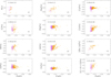 |
Fig. B.1 A(Li), [C/Fe], [N/Fe], [O/Fe], [Na/Fe], [Mg/Fe], [Al/Fe], [Ca/Fe], [Si/Fe], [Ce/Fe], [⟨Ba, La⟩/Fe], and [(C+N+O)/Fe] vs. [Fe/H] of the middle stream. Violet and orange dots indicate AI and AII stars, respectively. The numbers reported in the panels illustrate the Spearman’s correlation coefficient and its associated error. |
Appendix C Table scheme of the chemical evolution of ωCen
In this Appendix, we provide a table that summarizes the proposed scenario in Section 6. The identified populations are ordered chronologically from the first to the last row. The Table also provides a summary of the observed chemical features and their origin according to our scenario.
Summary of the timeline, the chemical features, and the origin of the different populations in ωCen.
All Tables
Summary of the timeline, the chemical features, and the origin of the different populations in ωCen.
All Figures
|
Fig. 1 Chromosome maps (ChMs) of the innermost two arcmin of ωCen published by (Milone et al. 2017) (left panel) and of the 2–5 arcmin region constructed from the HST catalog of Häberle et al. (2024) (right panel). The 1P, 2P, AI, and AII stars are shown in green, violet, blue, and orange, respectively. The two dot-dashed black lines separate the lower, middle, and upper streams in each panel. Black crosses mark stars that are present in our spectroscopic dataset presented in Section 2. |
| In the text | |
|
Fig. 2 Color–magnitude and radial-velocity diagrams of G vs. GBP-GRP from Gaia photometry. Gray points represent ωCen members with high-quality photometry, while black dots indicate the RGB stars with available APOGEE abundances, who reach up to ~30 arcmin radius. The inset shows the ΔDEC vs. ΔRA position respect to the cluster center (in arcmin) of the stars shown in the CMD. The top panel displays the radial velocity histogram of the selected sample of stars. |
| In the text | |
|
Fig. 3 Panel a: diagram of APOGEE [Al/Fe] vs. [Fe/H] for RGB stars in ωCen. Panel b1: zoom-in on the iron-poor end. Stars with ChM tagging are colored according to their assigned population, while the vertical dot-dashed line marks the 90th percentile of the 1P-star [Fe/H] distribution. Panel b2: normalized kernel-density distribution of [Al/Fe] for all stars (black) and for 2P stars (violet). The two dot-dashed horizontal green lines indicate the [Al/Fe] range of 1P stars. Panel c: same as panel b1 but zoomed on higher [Fe/H]. Panel d: [Al/Fe] vs. [Fe/H] For APOGEE stars located beyond 5 arcmin, colored according to the population tagging described in Section 3.2. The black lines mark the boundaries between the three streams, as reported in the plot. |
| In the text | |
|
Fig. 4 [Al/Fe] vs. [Fe/H] diagram, as in Figure 3, with probable binaries highlighted by cyan diamonds. |
| In the text | |
|
Fig. 5 Fraction of 2P stars relative to the total amount of canonical stars (top), AII stars relative to the bulk of anomalous (middle), and AI stars relative to the entire lower stream (bottom) plotted against the radial distance from the center of ωCen. Circles indicate fractions derived from the combined dataset, while triangles denote the APOGEE dataset only (see text for details). Diamonds represent fractions from binaries stars only. Gray lines show the radial intervals relative to each measurement, while the dot-dashed black lines mark the core and half-mass radii. |
| In the text | |
|
Fig. 6 elemental abundances A(Li), [C/Fe], [N/Fe], [O/Fe], [Na/Fe], [Mg/Fe], [Al/Fe], and [Si/Fe] vs [Fe/H] for lower-stream (panels a1-h1) and upper-stream (panels a2-h2) stars. Green, purple, violet, and orange dots represent 1P, AI, 2P, and AII stars, respectively. The numbers reported in the panel indicate the Spearman’s correlation coefficient and its associated uncertainty. |
| In the text | |
|
Fig. 7 Same as Figure 6 but for [Ca/Fe] of lower- and upper-stream stars (upper and middle panel, respectively), and [α/Fe] vs. [Fe/H] for 1P and AI stars (lower panel). |
| In the text | |
|
Fig. 8 Same as Figure 6 but for [Ce/Fe] (upper panels), [⟨Ba, La⟩/Fe] (middle panels), and [(C+N+O)/Fe] (lower panels) vs. [Fe/H] for lower- and upper-stream stars. |
| In the text | |
|
Fig. 9 Median A(Li), [C/Fe], [N/Fe], [O/Fe], [Na/Fe], [Mg/Fe], [Al/Fe], [Si/Fe], [Ca/Fe], [Ce/Fe], [⟨Ba, La⟩/Fe], and [(C+N+O)/Fe] vs. [Fe/H] of 2P (violet) and AII (orange) middle-stream stars. The continuous and dashed gray lines mark the average trends of the lower and upper streams, respectively. |
| In the text | |
|
Fig. 10 Distribution of nine abundance ratios (see labels) vs. [Fe/H] for lower-stream stars, compared with CCSN yields from a simulated population, whose initial composition is indicated by the open black dots. The blue square and red triangle indicate yields derived from the tables of Limongi & Chieffi (2018) and Nomoto et al. (2013), respectively. |
| In the text | |
|
Fig. 11 Diagram of [Al/Fe] vs. [Fe/H] showing middle-stream AII stars highlighted by orange bullets (panel a). Panels a1, a2, and a3 present the same plot zoomed in around seq1, seq2, and seq3, respectively (see text), with lower-stream stars highlighted for reference. The best-fit fiducial lines are shown in red, with open and filled red symbols representing the 0% and 100% dilution points, respectively. Panels b, b1, b2, and b3, show the corresponding plots in the [Mg/Fe] vs. [Fe/H] plane. |
| In the text | |
|
Fig. B.1 A(Li), [C/Fe], [N/Fe], [O/Fe], [Na/Fe], [Mg/Fe], [Al/Fe], [Ca/Fe], [Si/Fe], [Ce/Fe], [⟨Ba, La⟩/Fe], and [(C+N+O)/Fe] vs. [Fe/H] of the middle stream. Violet and orange dots indicate AI and AII stars, respectively. The numbers reported in the panels illustrate the Spearman’s correlation coefficient and its associated error. |
| In the text | |
Current usage metrics show cumulative count of Article Views (full-text article views including HTML views, PDF and ePub downloads, according to the available data) and Abstracts Views on Vision4Press platform.
Data correspond to usage on the plateform after 2015. The current usage metrics is available 48-96 hours after online publication and is updated daily on week days.
Initial download of the metrics may take a while.