| Issue |
A&A
Volume 705, January 2026
|
|
|---|---|---|
| Article Number | A184 | |
| Number of page(s) | 11 | |
| Section | Astrophysical processes | |
| DOI | https://doi.org/10.1051/0004-6361/202556619 | |
| Published online | 19 January 2026 | |
Fast and “lossless” propagation of relativistic electrons along magnetized nonthermal filaments in galaxy clusters and the Galactic Center region
1
Max Planck Institute for Astrophysics Karl-Schwarzschild-Str. 1 D-85741 Garching, Germany
2
Space Research Institute (IKI) Profsoyuznaya 84/32 Moscow 117997, Russia
3
Minnesota Institute for Astrophysics, University of Minnesota 116 Church St SE Minneapolis MN 55455, USA
4
Universitäts-Sternwarte, Fakultät für Physik, Ludwig-Maximilians-Universität München Scheinerstr.1 81679 München, Germany
5
Istituto Nazionale di Astrofisica (INAF) – Istituto di Radioastronomia (IRA) Via Gobetti 101 40129 Bologna, Italy
6
Rudolf Peierls Centre for Theoretical Physics, Department of Physics, University of Oxford Oxford OX1 3PU, United Kingdom
7
Merton College Oxford OX1 4JD, United Kingdom
★ Corresponding author: This email address is being protected from spambots. You need JavaScript enabled to view it.
Received:
27
July
2025
Accepted:
17
November
2025
Abstract
Relativistic leptons in galaxy clusters lose their energy via radiation (synchrotron and inverse Compton losses) and interactions with the ambient plasma. At z ∼ 0, pure radiative losses limit the lifetime of electrons emitting at ∼GHz frequencies to tr ≲ 100 Myr. Adiabatic losses can further lower Lorentz factors of electrons trapped in an expanding medium. If the propagation speed of electrons relative to the ambient weakly magnetized (plasma β ∼ 102) intracluster medium (ICM) is limited by the Alfvén speed (va,ICM = cs,ICM/β1/2 ∼ 107 cm s−1), GHz-emitting electrons can travel only 1 ∼ va,ICMtr ∼ 10 kpc relative to the underlying plasma. However, elongated structures spanning hundreds of kiloparsecs (or even a megaparsec) have been observed, requiring either a re-acceleration mechanism or another form of synchronization (e.g., via a large-scale shock). We argue that filaments with ordered magnetic fields supported by nonthermal pressure are characterized by va ≫ va,ICM and, thus, they can provide such a synchronization even without re-acceleration or shocks. In particular, along quasi-stationary filaments, electrons can propagate without experiencing adiabatic losses, and their velocity is not limited by the Alfvén or sound speeds of the ambient thermal plasma. This model predicts that along filaments that span significant pressure gradients (e.g., in the cores of galaxy clusters), the synchrotron break frequency, νb ∝ B, scales with the ambient gas pressure as P1/2. The emission from such filaments should be strongly polarized due to the magnetic field being ordered along them. While some of these structures can be observed as “filaments” (i.e., long and narrow bright structures), others can be unresolved and appear as a diffuse emission. They could also be too faint to be detected, while continuing to provide channels for electron propagation. We examine several cases of filamentary structures in tailed radio galaxies and in a cluster relic, where “lossless” propagation provides an attractive alternative to other mechanisms for explaining the observed spectral behaviors.
Key words: acceleration of particles / diffusion / magnetic fields / plasmas / radiation mechanisms: non-thermal
© The Authors 2026
 Open Access article, published by EDP Sciences, under the terms of the Creative Commons Attribution License (https://creativecommons.org/licenses/by/4.0), which permits unrestricted use, distribution, and reproduction in any medium, provided the original work is properly cited.
This article is published in open access under the Subscribe to Open model.
Open access funding provided by Max Planck Society.
1. Introduction
There are many examples of synchrotron-powered radio sources with complicated filamentary structures (see Fig. 1) that are becoming more and more commonly known as high-sensitivity radio observations become routinely available. They include the nonthermal filaments (NTF, e.g., Yusef-Zadeh et al. 1984) in the Calactic Center and filaments in the cores of galaxy groups and clusters (see, e.g., Owen et al. 2000, for examples of filamentary structures in the radio lobes of M87), as well as radio relics in the outskirts of galaxy clusters (see van Weeren et al. 2019, for a review) and the tails of radiogalaxies (e.g., van Weeren et al. 2024).
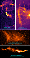 |
Fig. 1. Examples of radio-bright filaments in clusters and the Galactic Center, where fast propagation of relativistic electrons might be important. Top: Core of Nest200047 group, (left, Brienza et al. 2021, LOFAR image at 144 MHz) and the Galactic Center nonthermal filaments (right, Heywood et al. 2019, MeerKAT image at 1.3 GHz). Middle: Peripheral radio relic at the edge of the X-ray halo in Abell 2256 (Owen et al. 2014, VLA image at 1.5 GHz). In all cases, the filaments are long, comparable to the characteristic size of the system. They appear “laminar” and from the polarization measurements in the GC and Abell 2256, the magnetic fields are oriented along the filaments (e.g., Paré et al. 2019; Clarke & Ensslin 2006). In the case of the Galactic Center, we also know that the field is dynamically strong (e.g., Morris 2006). Bottom: Tailed radio galaxy, MysTail in Abell 3266, showing three parallel 40–50 kpc long filaments embedded in the tail. The host position is marked with an “X”. |
Diffusive shock acceleration (DSA) mechanism (e.g., Krymskii 1977; Blandford & Ostriker 1978; Bell 1978) predicts a power-law spectrum of accelerated relativistic particles dN/dγ ∝ γ−p, up to very high energies, and it is plausibly responsible for the production of relativistic electrons in these objects. In addition to acceleration by large-scale shocks, active galactic nuclei (AGNs) release accelerated relativistic particles into the ICM, either through directed flows or escape from old radio galaxy structures. Without re-acceleration, these electrons should lose their energy due to synchrotron radiation, inverse Compton (IC) scattering, adiabatic losses, and interaction with ambient plasma. Since the radiative losses depend strongly on the particle energy (∝γ2), a high-energy cutoff develops in the particle spectrum, which reveals itself in the observed synchrotron spectra. This break can be used to infer the “age” of the particle distribution if the magnetic field is known and no additional re-acceleration is taking place. The adiabatic losses scale linearly with γ and, therefore, they do not introduce a break in the particle spectra, but merely shift the existing energy break (if any). While “aged” spectra are commonly seen, there are cases when the inferred age is shorter than the estimated dynamic age of the source or the timescale for electrons’ streaming along the magnetic field with velocities lower than the Alfvén speed in ambient thermal plasma (e.g., Zweibel 2017). While various explanations for these discrepancies have been suggested (including a possibility of re-acceleration; e.g., Pacholczyk & Scott 1976; Brunetti et al. 2001; Petrosian 2001), we discuss below a set of conditions that might simultaneously lead to the minimization of losses and fast propagation of electrons along filamentary structures.
Here, we provide a few examples of objects featuring long and narrow filaments of synchrotron emission, and where the simplest estimates of the age and losses often appear in tension with observations.
The first group of such objects includes rising bubbles and filaments of relativistic plasma in the cores of galaxy groups and clusters; for instance, M87 (Owen et al. 2000), Nest200047 (Brienza et al. 2021, 2025, see Fig. 1), and Abell 194 (Rudnick et al. 2022), to name a few. Typical sizes of these radio-bright structures are in the range from tens to a couple of hundred kpc (the most prominent structure in the Nest200047 has a projected length of ∼350 kpc). Their age estimates can be based on the dynamics of buoyant bubbles (e.g., Gull & Northover 1973; Churazov et al. 2000; Zhang et al. 2018), which move down the pressure gradient of approximately hydrostatic atmospheres with velocities ≲cs, ICM. For instance, in the Nest200047 group (Brienza et al. 2025), the estimated dynamic age of some of the structures is t ∼ 200 kpc/500 km s−1 ∼ 4 × 10⁸ yr. Fitting the shape of the observed radio-band spectra in selected regions (assuming magnetic fields ∼2 μG, see Sect. 2.2) yields a shorter age by a factor of ∼2 when pure radiative losses are considered. We note that this factor of 2 does not look irrefutable, but once the adiabatic losses are added and the magnetic field pressure is set to values comparable to the gas thermal pressure, the discrepancy reaches almost an order of magnitude.
Another group of objects that might be affected by fast propagation of electrons includes very long tails of radio galaxies, for instance, 3C129 (Jaffe & Perola 1973; Pacholczyk & Scott 1976), Tail C in Abell 2256 (Owen et al. 2014), and the tail in the south of A1033 (de Gasperin et al. 2017). There, a prominent steepening of the spectrum is very clear in the vicinity of the AGN, but the spectrum flattens and stays relatively constant toward the end of the tail. A long tail in Abell 3266, on the periphery of the X-ray emission, shown in Fig. 1, displays similar behaviors.
The third group consists of radio relics (see, e.g., van Weeren et al. 2019, for a review). One of the best and earliest known relics to show long, prominent filamentary structures is Abell 2256 (Bridle & Fomalont 1976), which is also shown in Fig. 1. These structures are very likely created by merger shocks, which accelerate and/or re-accelerate relativistic particles. Relics have integrated radio spectra with the spectral index approaching −1. Here, the spectral index  , where Sν ∝ να is the emission spectral energy density. In the context considered here, α is always negative, consistent with an optically thin plasma emitting synchrotron radiation. At the same time, the modest values of shock Mach number inferred from X-ray surface brightness jumps suggest (in the DSA framework) steeper indices. The most actively discussed scenario explains these relics’ properties by strong dependence of electrons’ acceleration efficiency on the shock Mach number (e.g., Kang et al. 2019) coupled with variations of the shock Mach number on small scales seen in numerical simulations (e.g., Wittor et al. 2021; Dominguez-Fernandez et al. 2021; Whittingham et al. 2024; Lee et al. 2025). These variations can be associated with density or velocity fluctuations in the ICM or with multiple shocks Inchingolo et al. (2022). Some of these relics feature bright filamentary structures with relatively constant spectra along them. The Toothbrush relic presents another version of this puzzle: there, the integrated spectra have strikingly similar slopes (Δα ≈ 0.03) along the entire structure spanning 1–2 Mpc (Rajpurohit et al. 2020). If parts of the relic are interconnected by a network of filamentary structures, the fast propagation of electrons can contribute to the uniformity of the spectra. In this case, the spectrum slope may depend on the Mach number distribution in the entire structure.
The last example deals with the 10–100 pc-long nonthermal filaments (NTFs) in the Galactic Center, including the famous radio arc (e.g., Yusef-Zadeh et al. 1984; Heywood et al. 2019, see Fig. 1). In some of these filaments, which are possibly powered by pulsar wind nebulae (PWNs, e.g., Wang et al. 2002; Bykov et al. 2017; Barkov et al. 2019; Thomas et al. 2020; Yusef-Zadeh et al. 2024), high Lorentz factors of particles and a strong magnetic field produce synchrotron emission in the X-ray band. The lifetime of such particles is short (∼30 yr assuming dynamically important magnetic field), and the length of observed structures requires the propagation velocity to be a fraction of the speed of light (Wang et al. 2002; Zhang et al. 2020; Churazov et al. 2024). The X-ray emission is strongly polarized, close to the maximal possible polarization of the synchrotron emission in a uniform field aligned with the direction of filaments. Some NTFs form a sequence of almost equidistant parallel filaments (e.g., LaRosa et al. 2001). The length of individual filaments decreases monotonically in the direction perpendicular to filaments (see, e.g., Fig. 8 in Heywood et al. 2022), forming an overall shape resembling a triangle (sometimes called a “harp”). The central part of the Radio Arc in Fig. 1 also features a triangle-shaped extension that points toward a PWN. In the model of Thomas et al. (2020), these structures are due to the propagation of leptons (the leading front) with the Alfvén speed va ∼ 40 km s−1, while the source of the leptons is at the tip of the triangle. In this case, the shape of the “triangle” (half-angle typically larger than 45 degrees) bears partial analogy1 to the Mach cone of a supersonic jet, suggesting that the source is moving at a velocity comparable to or lower than va. This would be consistent with one of their models, where massive stars with velocities of a few tens of km s−1 produce leptons. However, the leptons might come from PWNs (our preferred model), which have an order of magnitude (or more) higher velocities and, therefore, the propagation speed of leptons has to be proportionally higher – at least a few 100 km s−1 independently of the details of the particle propagation mechanism. This value is much higher than the sound or Alfvén speeds in the ISM.
Here, we shall assume that all filamentary objects in these diverse groups share the same properties (a strong magnetic field aligned along the low-density filaments) and argue that in these conditions, relativistic electrons can propagate very rapidly and experience minimal losses. While another mechanism, such as re-acceleration (e.g., Pacholczyk & Scott 1976; Brunetti et al. 2001; Petrosian 2001), might be responsible for maintaining long-lived synchrotron emission in the bulk of the ICM, here we discuss situations where lossless propagation plays an attractive, plausible role.
Unless stated otherwise, we consider a filament of length, L, supported by a strong magnetic field, Bf. It is embedded in thermal plasma with gas pressure, Pt ∼ Bf2/8π. Here and below, quantities with subscripts f and t refer to the filament and ambient thermal plasma, respectively. We further assume that the filament contains relativistic particles and, possibly, some amount of thermal gas, with mass density much smaller than the density of the ambient thermal plasma, ρf ≪ ρt. With these assumptions, βf ≲ 1 or, possibly, βf ≪ 1. In the latter case, the magnetic pressure dominates inside the filament, while in the former, it makes up half of the filament pressure. In all cases considered here, we assume that the total pressure, Pparticles + B2/8π, in the filament is approximately equal to the ambient medium (ICM) pressure. This might not be the case for overpressurized bubbles in the proximity of an AGN in cluster cores, which drive shocks in the ambient gas. Such objects are not considered here. “Our” filaments could be advected by the ICM motions, expanding or contracting to maintain an approximate pressure equilibrium with the ambient gas.
2. Losses
Ignoring Coulomb losses, which that are not dramatically important for particles with γ ≳ 104 (e.g., Sarazin 1999; Petrosian 2001) that are of interest for this study2. We briefly discuss the radiative and adiabatic losses below.
2.1. Adiabatic losses
This section considers adiabatic losses of relativistic particles in isolation from all other possible losses. We first consider the case when particles are trapped in the tangled magnetic field of the slowly expanding Lagrangian fluid element with volume, V. We further assume that some level of scattering is present, so the pitch-angle distribution remains isotropic. Such particles should suffer from adiabatic losses. The Lorentz factor of particles changes as γ ∝ V1 − Γ, where Γ = 4/3 in the ultrarelativistic limit. If there is a break in the electron distribution function at γb, it will move down accordingly. We further assume that the energy density of the magnetic field also goes down with expansion, for instance, for a tangled field, Bf ∝ V−2/3. With these assumptions, the break frequency in the observed synchrotron spectrum evolves as νb ∝ γb2Bf ∝ V−4/3. This is relevant, for example, for buoyant bubbles of relativistic plasma in cluster cores (Churazov et al. 2001). If the bubbles are in pressure equilibrium with the ambient gas, then their volume  , where Γ is again 4/3, so νb ∝ Pt. Accordingly, as the bubbles move down the pressure gradient, the decrease of the break frequency should follow the drop of pressure (or faster if radiative losses are important).
However, if there is a pre-existing filament (i.e., a “channel”) that is stationary, then in the test-particle regime, there are no adiabatic losses for a particle propagating along the channel. This remains valid independently of the presence or absence of pitch-angle scatterings by spatially fluctuating magnetic field or changes of the medium’s energy density (and, hence, pressure) along the filament. This is also true if the filament is wider at one end and narrower at the other. What matters is that the scattering centers, on average, do not move away from the particle. This configuration closely resembles the model of tailed radio sources by Jaffe & Perola (1973), where the tail associated with a high-speed galaxy is replaced with a filament. In that model, the adiabatic losses are explicitly neglected (see also Pacholczyk & Scott 1976, for a different model). In the application to our hypothetical filaments, we note that the amount of adiabatic losses experienced by particles during a single journey along the filament can be linked to the change in the filament volume during that journey. Therefore, if the particle can propagate fast enough (so that the filament volume only changes by a small amount), the changes in the particle’s Lorentz factor along the filament associated with adiabatic expansion will be small as well (even though all particles do lose energy on the filament-expansion time scale)3. In other words, the adiabatic losses are inevitable, but they are not necessarily reflected in the shape of the electron spectrum along the filament.
2.2. Synchrotron and IC losses
These losses are set by the energy density of the magnetic and radiation fields4,
 (1)
(1)
assuming the pitch angle isotropization is faster than the cooling losses, where σT is Thomson cross section, c is the speed of light, and Urad is the energy density of radiation. Unlike the adiabatic losses that vanish for a stationary filament (Sect. 2.1), radiative losses are inevitable.
The longest lifetime of particles emitting at a given frequency is achieved (van der Laan & Perola 1969) when
 (2)
(2)
If the radiation energy density is dominated by CMB photons, then the upper limit on the particle lifetime is
 (3)
(3)
where z is the redshift and νc can be derived from the observed spectra5. For z = 0, we see that B1 ∼ 1.9 μG, while for weaker or stronger B, the lifetime will be shorter. This argument is often used to place an upper limit on the age of a synchrotron source or on the distance, d ≲ v tmax, which electrons can travel with the velocity, v.
The only way to reduce the aging of the electron population with the distance along the filament from the acceleration site is to increase the propagation velocity of electrons (or invoke a re-acceleration mechanism; e.g., Pacholczyk & Scott 1976; Brunetti et al. 2001). In particular, the assumption that particle velocities are limited by the Alfven speed, cs, t/βt1/2, in thermal plasma (βt ∼ 102) implies that at GHz frequencies the aging is important on scales ∼10 kpc and up to ∼100 kpc if the electrons are advected with trans-sonic velocities.
Since we consider here a “strong-field” case (i.e., Bf2/8π ∼ Pt), it is interesting to note that near the virial radius of present-day clusters, the corresponding value of Bf would be ∼μG; therefore, the energy density of the magnetic field in such filaments will be comparable to the CMB energy density. These conditions maximize the lifetime of particles emitting at a given frequency, implying that objects like radio relics might be visible for a long time (Churazov et al. 2023a). In contrast, in the cluster cores, the “strong-field” condition corresponds to Bf ∼ 20 − 50 μG, synchrotron losses dominate the particles’ aging and the lifetime of particles emitting at a given frequency is relatively short.
We illustrate the expected magnitude of the combined adiabatic and radiative losses on the spectrum of a subsonically rising “bubble” in the core of the Nest200047 group in Fig. 2. This object has a large linear size of AGN-powered radio structures (Brienza et al. 2021) and a steep radial pressure profile, while the thermal gas temperature is modest at ∼2 keV. This makes this object particularly suitable for getting the most stringent constraints on the electrons’ losses associated with long rise time (radiative losses) and large pressure gradient (adiabatic losses). From this figure, it is clear that a combined action of adiabatic and radiative losses for Bf2/8π = Pt would lead to a very steep spectrum (the blue curve in Fig. 2) at a distance of 140 kpc from the core. In Brienza et al. (2025), the lack of very strong steepening is discussed in terms of the re-acceleration scenario. Here, we consider an alternative possibility: low-beta filaments, which in the most optimistic scenario can eliminate these losses (see the red curve in Fig. 2). Essentially, the blue and red curves correspond to the maximal- and minimal-loss scenarios, respectively, and the difference in the predicted spectra is large. In this study, we focus on the latter scenario. In this (minimal-loss) limit, the spectrum of electrons is the same over the entire filament. Therefore, in the observed synchrotron emission, the break frequency varies along the filament solely due to variations of B sin θ, where θ is the angle the magnetic field makes to the line of sight.
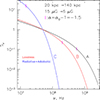 |
Fig. 2. Expected steepening of synchrotron spectra as particles move from the cluster core in the radial direction from 20 to 140 kpc. All spectra are normalized to unity at ν = 5 × 10⁷ GHz. The magnetic energy density is assumed to follow the ICM pressure profile Pt(r), i.e., Bf2/8π = Pt(r). For these simulations, we adopted a simple power law pressure profile Pt ≈ 2 × 10⁻¹⁰(r/kpc)−1 erg cm−3, derived from X-ray observation of the NEST200047 group (Majumder et al. 2025). The solid back curve (marked A) shows the synchrotron spectrum at the initial position at r1 = 20 kpc. It has a low-frequency slope α0 = −0.5 and is “aged” in the 15 μG field for 3 × 10⁷ yr so that a break develops in the spectrum. The spectra marked B and C show the evolved spectra at the final position at r2 = 140 kpc. These spectra represent two extreme limits. In particular, for C, the electrons are moving “in a bubble” from r1 to r2 with the velocity v = 500 km s−1 (just below the sound speed in the group ICM cs ∼ 700 km s−1) and suffer from the adiabatic and radiative losses. In addition to the evolution of the particle spectrum, the magnetic field is lower at r2. All these effects combined lead to a very steep spectrum at the final position. In contrast, for the “B” spectrum, we assume that electrons quickly propagate “along a static filament” and do not suffer from any losses. The only reason why the spectrum B is steeper than A is that the magnetic field is lower at the final position; hence, a lower critical frequency, νc ∝ B. For each curve, the position of the break frequency (defined here as a frequency where the spectral slope is α = α0 − 1) is shown with a small vertical magenta bar. This plot illustrates that if the initial spectrum has a break around 1 GHz, and no re-acceleration is present, any “subsonic” regime of propagation (blue lines) will result in a very steep spectrum at 100 MHz. If “fast-track” routes are available for a fraction of electrons, this might reduce the apparent steepening dramatically. |
Yet another convincing example of a competition between radiative losses and rapid propagation comes from PWNs. X-rays from the “misaligned” filaments associated with pulsar wind nebulae provide solid evidence that on scales of ∼1 − 10 pc, relativistic leptons (with γ ∼ 108) propagate with the velocity of at least ∼104 km s−1 (e.g., Kargaltsev & Pavlov 2008; Klingler et al. 2023; Dinsmore & Romani 2024). This follows from the synchrotron cooling time estimates and the observed length of the filaments. The motion of the ∼ parsec-long X-ray-bright filament together with the PWN in the Guitar Nebula (see Fig. 4 in de Vries et al. 2022) over 20 years corroborates this conclusion. In fact, if the length of these filaments is set not by cooling time but by the changes in the filaments’ geometry and properties, the velocity should be even higher than estimated using the observed length and Eq. (3). For instance, the filament might transition to a high-β type at its end, effectively preventing further fast propagation of particles by enhancing the scattering rates (as in Ewart et al. 2024). In this case, particles might be able to travel back and forth along the filaments, erasing gradients associated with radiative cooling along filaments. The equipartition fields in these objects are not dissimilar from the values that can be found in clusters (assuming B2/8π ∼ Pt). However, for electrons emitting at frequencies ∼1 GHz, the same propagation velocities would translate into distances of ∼100 kpc over their longer radiative cooling time.
2.3. Interactions with plasma waves
Another process pertinent to the propagation of particles is the interaction with plasma waves, which can scatter relativistic particles (Kulsrud & Pearce 1969; see, e.g., Zweibel 2017; Ruszkowski & Pfrommer 2023 for reviews). The condition of the strong field in the filament adopted here implies that external driving, for instance, turbulence in the ICM, is unlikely to affect the fields on scales comparable to gyroradii of relativistic electrons. In the test-particle regime, the relativistic electrons will stream (Skilling 1975) along the filament with a velocity on the order of c. However, it is often assumed that streaming particles excite waves that, in turn, scatter these particles. In the absence of other damping mechanisms, the waves (and the particles’ scattering rate) grow until the streaming velocity drops below the local Alfven speed. Such a process can dramatically reduce the cosmic rays’ propagation speed away from the source in the ICM or ISM.
In a strong-field nonthermal filament, however, the Alfvén speed vA,f can be very high, much higher than the Alfvén speed, vA,t, in the ambient high-β plasma or its sound speed, cs. In fact, vA,f can be as high as O(1)c if the filament is completely devoid of thermal gas. This has important implications. Since the filament itself is supposedly created (see Sect. 2.1) on timescales on the order of (or longer than) the sound crossing time in the ambient plasma, this means that the gradient of relativistic particles’ energy density along the filament will be small during the formation of the filament. The second implication is that, once the filament is formed, the gradients caused by any additional injection of fresh particles will be erased quite quickly; alternatively, if the streaming velocities fall below vA,f, the streaming instability will not be triggered at all. In any case, a high Alfvén speed implies that both adiabatic and radiative losses on the time scale of particles’ propagation along the filament are small. Therefore, the situation where there is no difference in the “effective age” of the relativistic electrons’ distribution along the filament can naturally occur.
3. Formation and “survival” of filaments
The exact set of necessary and sufficient conditions needed to provide fast transport of relativistic electrons along filaments is not clear. Given that the gas motions in the ICM are predominantly subsonic, we would not expect to see β ∼ 1 in the bulk of the gas, although in some special conditions (e.g., a merger of two clusters and/or strong and sustained shear), patches of low β ∼ 1 might be formed, driving vA closer to cs, t. Based on the premise that velocities much higher than cs are required, the mass density in the filaments has to be much lower than that of the ICM. In this case, AGN-produced plasma becomes the most viable candidate (as we also argue in Sect. 5). Therefore, it is interesting to consider what fraction of volume could, in principle, be filled with such plasma. If we take a typical cool-core cluster with the cooling radius of rcool ∼ (0.1 − 0.2) R500c (i.e. ∼100 − 200 kpc), the amount of energy supplied by the central AGN during the Hubble time would be on the order of the ICM thermal energy within the cooling radius. Assuming that all this energy is supplied in a nonthermal form and all ICM heating (AGN Feedback) is in fact set by “mechanical” interactions with nonthermal plasma (Churazov et al. 2000), namely, it is effectively produced via adiabatic losses, the fraction of volume filled by nonthermal plasma within R500c is between 2 and 10%. This is, of course, a very crude estimate, but it shows that this fraction can be substantial. A much more difficult question is related to what happens to this nonthermal plasma. For instance, it could eventually be dispersed and mixed with the thermal ICM. Observations suggest that at least in the cores of clusters, there are “filament-like” structures that are a few 100 kpc long, which suggests a lifetime of more than 100 Myr (for velocities ∼cs, t). The question of whether they can survive longer remains open and we further comment on the implications of this possibility in Sect. 5.
4. Examples of observational constraints on electron propagation velocities in visible filamentary structures
In this section, we provide examples where very high transport velocities for the radiating relativistic electrons provide a plausible explanation for the observed spectral structures. These include very different astrophysical situations, all associated with galaxy clusters: tailed radio galaxies and peripheral relics associated with merging clusters. In each case, alternate explanations are also possible, such as distributed acceleration, but here our emphasis is on presenting the attractive possibility that fast electron transport is occurring.
Using Eq. (3), we find that if the travel distance, d, of the electrons is measured and the amount of radiative aging over that distance is characterized by a quantity, tobs, calculated from the change in the cutoff frequency in the spectrum, then a minimum electron velocity vmin can be derived. To do this, we assume that the time of observation, tobs, is equal to the maximum lifetime, tmax, for the observing frequency. This yields a lower limit for the transport velocity of the electrons, v ≳ vmin = d/tmax.
4.1. Tailed radio galaxies
Here, we examine two tailed radio galaxies, where the basic model assumes that the relativistic particles are (almost) at rest in the ICM. The jets emerge approximately transverse to the direction of motion of the host through the ICM, and the jets are swept back and quickly come approximately to rest6. We look at two cases, Tail C in Abell 2256 (at z ≈ 0.058; Owen et al. 2014; Osinga et al. 2024) and the GReET source in Abell 1033 (de Gasperin et al. 2017).
Tail C is a 700+ kpc very narrow tail in the cluster Abell 2256 (Rottgering et al. 1994; Owen et al. 2014; Miller et al. 2003). The host is SDSS 17330.04+783955.4 (WISEA J170330.04+783954.3), with a radial velocity of 17558 ± 36 km s−1, nearly at rest along the line of sight with respect to the 17490 ± 74 km s−1 systemic cluster velocity. The cluster velocity dispersion is  (Miller et al. 2003). Tail C’s straightness and very long length have raised questions about how the host dynamics, or ongoing particle acceleration, could lead to the observations. Below, we re-examine the spectral behavior in the context of possible fast electron transport.
The high-resolution observations shown in Fig. 14 of Owen et al. (2014) reveal that the structure is unresolved transversely in the first kpc downstream, and then shows parallel strands beyond ∼30 kpc from the host. These strands are blended into a single long, thin structure at the 6.8″resolution used here. The presence of regions with parallel strands could be due to two very closely spaced tails or jet edge brightening, with Tail C actually being a unique, extreme, one-sided, high-velocity jet. For the analysis presented here, we do not explore this option and treat the source as either a single, left-behind tail or two blended parallel left-behind tails.
In Fig. 3, we plot the spectral index at a resolution of 6.8″ between 149 MHz (using a LOFAR map courtesy of R. van Weeren; see Osinga et al. 2024) and 1515 MHz, (using a VLA map as presented in Owen et al. 2014). From this, we can calculate the local cutoff frequency, νc, and, thus, tmax at each location, assuming an exponentially cut-off spectrum with a low-frequency index of −0.5, as observed near the host, and setting B1 = 2.26 μG (using Eq. (2) and the CMB energy density at the cluster redshift). The spectral index drops quickly (≲kpc) to approximately −0.6, and then more gently to about −0.85 at 70 kpc from the host. Further downstream, with some small but significant wiggles, the inferred tmax increases linearly with distance from the AGN. This is consistent with a constant velocity of the relativistic electrons (in the case of streaming) or of the host (in the case of flow being stopped in the ICM).
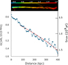 |
Fig. 3. Top: Map of Tail C in Abell 2256 at 6.8″resolution at 149 MHz, (LOFAR reference), color-coded by its spectral index to 1.5 GHz (Owen et al. 2014). Bottom: Observed spectral index between 149 and 1515 MHz, and the corresponding maximum age for relativistic electrons at each location, based on the cutoff frequency calculated from the spectral index, as described in the text. The red line corresponds to an electron transport velocity of 4500 km s−1. |
The relation between the slope of the spectral index and distance, converted to νc and tmax vs. distance, yields an inferred relativistic electron velocity vmin ∼ 4500 km s−1 due to radiative aging alone. This represents a minimum velocity because, if the velocity were lower, or if B ≠ B1, then much more aging would have occurred. The velocity vmin would have to be even larger than derived above if there were also adiabatic losses, or if the magnetic field weakened downstream. The brightness of the tail as a function of distance is approximately as expected from the spectral steepening alone. It is thus likely that the magnetic field is approximately constant in these first 400 kpc, so any weakening downstream does not contribute significantly to the change in spectral index.
If the tail were simply plasma at rest with the ICM, left behind after the passage of the host through this region, then the velocity of the host in the plane of the sky would have to be ≥ vmin. Since vmin is approximately 3.5 times higher than the cluster velocity dispersion, such a high projected velocity seems unlikely, although not impossible. Fast streaming of the relativistic electrons down the tail, as proposed here, offers a simple way of achieving the required minimum velocity and reducing radiative losses. Alternatives include a supersonic host velocity, the long-standing idea of in situ acceleration of the relativistic particles throughout the tail (Eilek 1982; de Oliveira et al. 2025), or that Tail C actually is a unique one-sided jet with a bulk flow of ∼4500 km s−1.
Another source with a remarkably constant spectral index in its downstream tail is found in the southern portion of Abell 1033 (hereinafter GReET, de Gasperin et al. 2017; Edler et al. 2022). The source is a “narrow-angle-tail” (NAT)7 that is similar, for instance, to NGC 1265. Far behind the host AGN, a larger than 200 kpc portion of the tail is displaced transversely, which is attributed to bulk motions in the medium, perhaps behind a weak shock. Such displacements are indeed seen in the simulations of O’Neill et al. (2019b), who introduce a shock moving perpendicular to a NAT tail.
From multifrequency observations and color-color diagrams (Katz-Stone et al. 1993), de Gasperin et al. (2017) and Edler et al. (2022) measure GReET’s injection spectral index to be –0.65. The spectra then steepen downstream to –2 (between 54 and 323 MHz) and –4 (between 144 and 323 MHz). Beyond 400 kpc, the spectral steepenings should continue even more dramatically, with continuing radiative losses, but this is not observed. de Gasperin et al. (2017) invoke “gentle reacceleration” via turbulence in the displaced portion of the tail to maintain a relatively constant, but steep spectrum. As noted by de Gasperin et al. (2017) this requires “a very special geometrical and physical configuration”. We estimate that local fluctuations in Mach number, if DSA were responsible, would need to be less than a few percent, which seems unlikely. Whether or not the turbulence has uniform enough properties over 100s of kpc to maintain the spectral shape is another aspect that could be useful to explore in this context. Here, we investigate the possibility that, instead, large electron velocities in this portion of the tail minimize the spectral steepening.
We performed a similar analysis as for Tail C as that described above. Figure 4 shows a plot of the spectral index between 144 and 323 MHz, taken directly from Fig. 3 of de Gasperin et al. (2017). Behind the host, the spectral index steepens from ∼ − 1.5 to ∼ − 4.5 in the first 350 kpc. With a constant magnetic field B1 = 2.4 μG (thus minimizing losses with  ) and a velocity of 700 km s−1, the observed steepening with distance would be reproduced. But after flattening to ∼ − 3.75 (discussed further below), the spectral index stays relatively constant for the final 200 kpc; it is this last section of the tail that we consider. Here, the maximum amount of steepening consistent with the data is from −3.75 to −4. Since we are in such a curved part of the spectrum, from the initial −0.65 power law, this corresponds to only a very small change in νc, from 72 MHz to 67 MHz. Again using B1 = 2.4 μG, this corresponds to a change in tmax from 375 Myr to only 389 Myr, giving vmin ∼ 15000 km s−1. Since this velocity is much higher than any plausible dynamical velocity in the system, fast electron transport becomes an attractive possible cause.
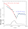 |
Fig. 4. Spectral index of the GReET tail in A1033 tail as a function of distance from the host, from Fig. 3 in de Gasperin et al. (2017). The red points show the expected steepening of an α0 = −0.65 spectrum with a low velocity for the radiating plasma, while the very modest amount of steepening in the final portion of the tail is consistent with a much higher transport velocity of 15 000 km/s, as shown in blue. The bottom plot, in solid black, shows the inferred direction of the host’s motion at each position in the tail, assuming the tail is left behind material. The variation in direction around 400 kpc is assumed to arise from a transverse flow, not from a change in the host velocity. |
The fast transport process alone does not explain the flattening of the spectral index between ∼375 and 400 kpc from the host. However, the tail is fainter in the steepest region, so that the magnetic field could be somewhat weaker there, then strengthening again as the brightness increases and the spectra flatten. Another interesting possibility is that the flattening arises not from a change in magnetic field, but from the bending of the tail along the line of sight. In Fig. 4 we plot the inferred direction of the host velocity in the plane of the sky; its initial trajectory is at∼ − 105°, then it curves by ∼60° as it is transversely displaced approaching 400 kpc, until returning to ∼ − 95°, close to its original direction. If this dramatic change in curvature were accompanied by only a 30° change in direction along the line of sight, this would cause the observed spectrum to flatten from –4.79 to –4.3, as observed. This occurs because the observed cutoff frequency is, in more detail, given by νc ∝ γc2B sin θ, where γc is the electron cutoff energy and θ is the angle to the line of sight. Thus, in the case of a strong ordered magnetic field, at a fixed observing frequency, the observed spectral indices from a curved spectrum depend on the angle of the field. The analysis above does not constitute proof that fast electron transport and possible jet bending are the cause of GReET’s spectral behavior; it does show that it is plausible.
A close analog to the spectral trends in GReET was recognized during the revision process, viz. the MysTail in Abell 3266 (Rudnick et al. 2021; Knowles et al. 2022; Riseley et al. 2022). Like GReEt, it is tangentially oriented in the periphery of the cluster X-ray emission. Its radio spectra steepen quickly with distance from the host for the initial 200+ kpc, followed by a fainter region of another 200+ kpc with little or no further spectral steepening (see Fig. 5 in Rudnick et al. 2021 and Fig. 13 in Riseley et al. 2022). Embedded in the tail are at least three prominent filaments connecting two diffuse patches of emission (Fig. 7 in Rudnick et al. 2021); other striking filaments are shown in their Fig. 10, connecting with the long tail in Abell 1314 (van Weeren et al. 2021).
4.2. Filaments in cluster relics
In this section we look at the northwest relic of Abell 3667, based on the data presented in de Gasperin et al. (2022). The relic is highly filamentary, with a mixture of short segments on scales of 102 kpc, and a number of much longer filaments, on Mpc scales, comparable to the size of the entire relic. Our Fig. 5 is a zoomed-in portion of their Fig. 14, revealing the wide range of spectral indices within the relic. One striking aspect of these spectral variations is that they appear well-correlated with the filamentary structures themselves – each filament has its own characteristic spectral index, along with some variations.
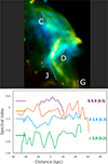 |
Fig. 5. Top: NW relic of Abell 3667 from de Gasperin et al. (2017). Colors indicate the spectral indices, and different filaments show different characteristic indices. Bottom: spectral indices along five of the filaments, showing how the variations along them are significantly smaller than the differences between them. Numbers on the right indicate the equivalent Mach numbers (and their scatter) if these indices were due to DSA. Errors per measured point are just slightly smaller than the variations, so the intrinsic variations are significantly smaller than observed. |
To look at this more quantitatively, we measured the spectral indices along the ridge line of several of these filaments, as shown in the bottom of Fig. 5. The average index of each of these filaments is significantly different than the others. The intrinsic spectral variations along these filaments are likely significantly smaller than observed, since there is an extensive network of overlapping structures and underlying diffuse emission of comparable brightness.
A complicated shock substructure is seen in many numerical simulations (e.g., Hoeft et al. 2008; Skillman et al. 2011; Wittor et al. 2017; Nuza et al. 2017; Roh et al. 2019; Dominguez-Fernandez et al. 2021; Inchingolo et al. 2022; Smolinski et al. 2023; Böss et al. 2023; Lee et al. 2025). In such a complex environment, the question is how to maintain a relatively constant spectral index along each filament. Their shapes and structures make it unlikely that the local Mach number remains strictly constant along each filament. The variations along the segment D, for example, would require Mach numbers constant to within ±8%. MHD simulations of relics show a wide range of Mach numbers within each relic (e.g., Böss et al. 2023; Lee et al. 2025), so the broad range of values observed here between different filaments is expected; what is surprising is the coherence of spectral indices over long distances within individual filaments.
One explanation for the observed spectral uniformity of filaments in A3667 is that any local variations in Mach number and particle acceleration have been homogenized due to fast transport along the filament. As long as the homogenized spectra are close to a power law over just a factor of a few in frequency, localized magnetic field variations will not lead to varying observed spectral indices. In the absence of significant radiative losses around the frequency of observation, we expect this to be the case. Higher-resolution observations at a range of frequencies would allow the spectra and spectral curvature of filaments to be disentangled from the various confusing structures and provide better constraints on their spectral uniformity.
Abell 2256 is another case where a prominent network of filaments fills the relic (e.g., Clarke & Ensslin 2006). Using the data in Owen et al. (2014), we attempted to trace the spectral variations along individual filaments, to see if they had distinct values. The variations along filaments, however, were of the same order as the difference between filaments, and therefore do not provide any evidence to support fast electron transport. However, since the filaments overlap with one another and are each embedded in more extended features, we could not conduct a clean test. It would be useful to experiment with a range of spatial filtering and tomographic analyses to see whether individual structures with distinct spectral indices could be isolated.
5. Discussion
The above considerations suggest that in a nonthermal filament with a strong field, the energy spectrum of relativistic electrons can be largely independent of the distance from the initial source of these electrons. A condition for such spectral uniformity is that the propagation time of electrons along the filament is shorter than both the radiative cooling time and the filament expansion time (dlnV/dt)−1, where V is the filament volume. Given that the Alfvén velocity vA,f in the filament can be high, this appears to be the easiest scenario that allows for “synchronizing” the electron populations emitting at ≲GHz frequencies over scales ∼0.1 − 1 Mpc in galaxy clusters. We also presented several examples of visible filamentary structures in clusters of galaxies where this could be taking place.
5.1. Formation of filaments
At this point, we want to consider how filaments with such properties end up being formed into clusters. As mentioned in Sect. 3, one natural scenario is related to AGN-inflated bubbles in cool-core clusters. Observations in radio and X-ray bands (e.g., Boehringer et al. 1993) show that these bubbles are bright in radio and dim in X-rays, suggesting that magnetic fields and relativistic particles are present, while the density of thermal plasma is significantly lower inside the bubbles. Even stronger limits come from observations of the SZ (Sunyaev & Zeldovich 1972) signal from the largest resolved bubbles in MS 0735.6+7421 (Abdulla et al. 2019; Orlowski-Scherer et al. 2022). The lack of the SZ decrement from these bubbles suggests that either they are devoid of thermal plasma or this plasma has a temperature higher than hundreds of keV. This makes AGN-inflated bubbles good candidates for plasma reservoirs with the required properties. These light “bubbles” evolve under the action of buoyancy (e.g., Gull & Northover 1973; Churazov et al. 2000) and move radially in cluster atmospheres down the pressure gradient and/or due to large-scale motions of ambient thermal plasma. Buoyancy naturally produces subsonic motions (e.g., Zhang et al. 2018) and can also stretch magnetic field lines that are anchored to the bubble and the gas in the core (e.g., Churazov et al. 2013). Once again, the subsonic velocity implies that an isolated bubble should suffer from radiative (and adiabatic) losses. However, once a filament is formed, the signs of both types of losses along the filament can diminish. This scenario can be relevant to objects like M87, Nest200047, Abell 194, and other clusters where a central AGN is present. Yet another scenario, involving a central AGN, was considered in Giacintucci et al. (2022) in application to the A3562 cluster. In this scenario, tangential flows along the contact discontinuity in the cluster core create an elongated filament. Once again, either reacceleration or fast propagation is needed to keep the radio spectrum uniform.
Another possibility is that filaments originate in the flows from one or more cluster noncentral AGNs. For example, in tailed galaxies, the AGN is still responsible for producing the initial volume of magnetized plasma, but the motion of the galaxy relative to the ICM produces a long “channel” with nonthermal plasma. Similarly to the original model of Jaffe & Perola (1973), the (strong) field becomes “straight” in the far tail, while in the vicinity of the source, it might remain turbulent and tangled.
A pre-existing population of filaments will also affect the appearance of radio relics. For relics, the presence of shocks is a strong argument for an acceleration (or re-acceleration) scenario. As in Churazov et al. (2023a), we argue that when accelerated (or re-accelerated) leptons appear in a preexisting filamentary structure with an ordered strong field, these leptons can quickly propagate along the entire structure. Once again, an AGN might be the initial source of these low-beta structures, further stretched and bent by the gas motions as, for instance, in the simulations run by of ZuHone et al. (2021).
On completely different physical scales, the Galactic Center NTFs could arise from stretching and ordering of the field by a global outflow from the central region (e.g., Heywood et al. 2019; Ponti et al. 2019). This demonstrates that conditions favorable for fast propagation are not endemic to clusters.
5.2. Testable predictions of the model
In this section, we discuss some possible testable predictions of the model discussed here. These include magnetic field topology, radio spectral properties and trends, and, possibly, IC emission.
5.2.1. Magnetic field orientation, degree of polarization, and Faraday rotation
First, a strong field aligned with the filament implies that the observed synchrotron emission should be strongly polarized. Indeed, for some filaments with measured polarization, the orientation of the electric field vector is perpendicular to the filament, and the degree of polarization is large (e.g., Yusef-Zadeh et al. 1984; Paré et al. 2019; Rudnick et al. 2022). A patch of the Radio Arc near the PWN candidate G0.13-0.11 features strong polarization (57 ± 18%) even in the X-ray band (Churazov et al. 2024), where Faraday rotation is negligible. This level of polarization, albeit with large uncertainties, is consistent with a highly ordered field. The same is true for tailed radio galaxies, as, for instance, the classic case of 3C129 (Miley 1973; Murgia et al. 2016) as well as newer examples (Müller et al. 2021).
Since this model assumes a low density of electrons inside filaments where synchrotron radiation is produced and the fields are highly ordered, no internal Faraday rotation is expected, and the fractional polarizations of filaments should be high, as is generally observed. In the one case where low-β conditions have been established from the presence of an X-ray cavity (the “E-fils” in Abell 194, Rudnick et al. 2022), the fractional polarizations are extremely high (1±0.25). In this case, the observed large coherent patterns in the Faraday rotation likely arise in the local surrounding medium. In Abell 194, the Faraday-corrected magnetic field angles trace well the local orientation of the filaments. Observations of magnetic field directions that were not along the filaments in some objects would also invalidate the model for them. Unfortunately, current X-ray instruments are not capable of detecting an excess of thermal emission due to filaments, because of limited angular resolution and sensitivity.
In the absence of depolarization, highly polarized filaments provide other opportunities for studying the intracluster medium. Faraday rotation patterns along a sufficiently long filament have distinct advantages in measuring the correlation length of the magnetic field in the ICM. It can also provide clues to the 3D structure of the filament, as suggested by Rudnick et al. (2022). An interesting additional consequence of this model, once proven, is that since the magnetic field would be parallel to the filament, measurements of the polarization angle at a single frequency would be sufficient to measure the Faraday rotation.
5.2.2. Shape of the synchrotron spectra
Second, if all energy losses of particles are indeed minimal, any existing break in the particle distribution does not change along the filament. This should be reflected in the shape of the observed synchrotron spectra. The persistence of the spectral shape can be studied through the use of color-color diagrams (Katz-Stone et al. 1993). In addition, if there is an independent way to connect the local magnetic field strength in the filament to the surrounding thermal pressure, then one can make predictions about the correlation between the observed filament brightness and the observed νb. An object such as the Nest20047 group (Brienza et al. 2025) may present such an opportunity. The condition of minimal losses for magnetically supported structures in cluster cores implies that the characteristic frequency of synchrotron radiation should scale as νb ∝ γ2Bf ∝ Pt1/2. This is in stark contrast with the maximal-losses scenario, when adiabatic and radiative losses “cooperate” on the background of slowly moving buoyant bubbles (see Fig. 2). The presence of emission regions with “young” spectra, some 100 kpc from the core, suggests that either re-acceleration or fast propagation mechanisms are involved. Discriminating between different scenarios might be nontrivial. Once again, a high degree of polarization might be particularly relevant for the fast-propagation scenario.
Yet another prediction relies on the possibility that leptons can go back and forth along a filament before they age. As discussed in Sect. 2.2, a possible configuration might involve a transition to a high-β phase at the end of the filament, where the scattering rate is large (e.g., Ewart et al. 2024; Reichherzer et al. 2025). Alternatively, the filament might be magnetically isolated from the ambient plasma so that the field lines are tangled at the end of the filament. If the leptons are added to the filament at different times, we should see a mixture of different ages at any given position. This implies that we should see not a simple single-age spectrum characterized by one break frequency but a gently curved shape. In this case, models that consider a distribution of ages (e.g., Komissarov & Gubanov 1994) might provide a better fit to the data than models that assume a single episode of particle acceleration.
In the model considered here, large-scale geometry is set by either buoyancy or the motion of an AGN relative to the ICM. At the same time, coherent radio structures are synchronized by the propagation of electrons along the field lines, while the cross-field diffusion is strongly suppressed. As a result, one can expect to see “bundles of threads” in the radio images with sufficient sensitivity and angular resolution. This is indeed observed for NTFs (e.g., Paré et al. 2019) and the filaments in clusters (e.g., Rudnick et al. 2022; Brienza et al. 2025; van Weeren et al. 2024; De Rubeis et al. 2025). However, the filaments locally are essentially “independent”, i.e., each of them is “synchronized” along its length but not necessarily with other filaments. As a result, individual filaments might be unresolved or too faint to be seen.
Even if the electron spectrum is homogenized along the filament and the pitch-angle distribution of electrons is isotropic, one can expect spectral variations due to the changes of the angle θ between the filament (= magnetic field) and the line of sight. In the ordered field, the intensity and critical frequency both depend on B sin θ. For a narrow filament, the increase of the line-of-sight length compensates for the decrease of intensity for small values of θ, but the critical frequency dependence on θ remains. Therefore, one can expect to find a correlation between the brightness and hardness of the spectrum, provided the cutoff frequency is not much higher than the observed range. Such a correlation will have the same signature as the variations of the age, except it reflects only the orientation of the filament. In this case, the dependence on the viewing angle might be nonmonotonic along the filament, and a correlation or anticorrelation of the flux and slope is possible. We speculate that in some extended radio sources (e.g., de Gasperin et al. 2017), this effect can explain the sudden hardening of the synchrotron emission further away from the primary source of electrons.
On a more speculative side, if the filaments are formed by large-scale motions stretching an initially compact region, magnetic field lines can reverse direction across filaments (see, e.g., Jaffe & Perola (1973) for radio tails or Churazov et al. 2013 for radio bubbles). Such structures might have weaker fields in the center, leading to edge-brightened “hollow-tubes” in radio emission. It is interesting to note that several “double-stranded” filaments are indeed seen in clusters (e.g., Brienza et al. 2021, see also our Fig. 1). A reversal in magnetic-field direction might be detectable by transverse gradients in Faraday rotation (Rudnick et al. 2024), when there is sufficient spatial resolution.
5.2.3. Long-living filaments and IC emission
If the filaments can survive without mixing with thermal gas for a long time (longer than the synchrotron cooling time of electrons emitting in the observable band), the ICM might be “infested” with filaments occupying a small volume fraction but present everywhere. In principle, the presence of such (long-living and most of the time invisible) structures might affect dynamical or transport properties of the bulk ICM plasma.
This might also affect the propagation of cosmic rays on spatial scales set by the sizes and morphologies of filaments embedded in the ICM. If relativistic protons make a significant contribution to the nonthermal pressure but are confined to filaments, no gamma-rays associated with π0 are expected (e.g., Prokhorov & Churazov 2017). On the contrary, the IC emission associated with relativistic leptons might be enhanced if these leptons are confined to nonthermal filaments with a small density of thermal electrons, effectively suppressing the Coulomb losses for the low-energy part of the particle spectrum. Indeed, in the majority of models (e.g., Sarazin 1999; Petrosian 2001; Hopkins et al. 2025), the Coulomb losses are calculated assuming a background density of electrons ne ∼ 10−3 − 10−2 cm−3. In the “filaments” model, the Coulomb losses are absent (or suppressed), and the peak of the aged distribution of relativistic electrons is either absent or shifted toward lower Lorentz factors. Since the Coulomb losses are suppressed, the nonthermal bremsstrahlung is absent, too. The synchrotron losses are instead high (in cluster cores, if magnetic field energy density is close to ICM pressure), further shifting the peak Lorentz factor to lower values. Therefore, in the no-mixing scenario, IC emission in the optical/UV band is possible, which might be relevant to the reported UV excess from clusters (e.g., Lieu et al. 1996), especially given that the (thermal and photonionization-induced) soft X-ray emission from the IGM predicted by numerical simulations is orders of magnitude fainter and has different radial dependence (Churazov et al. 2023b). However, to explain the reported UV luminosity relative to the observed radio luminosity, an aged electron population is required, as in several models discussed in Sarazin (1999), except that the break in the spectrum due to Coulomb losses can now be shifted toward lower Lorentz factors (or frequencies in the observed spectra).
5.3. Determining whether such objects are rare and the need for more observations
Finally, we address the question of why clear cases for lossless transport appear so rarely. In short, the main reason is that we have not yet looked for them, and there are few existing broad-band analyses spanning large variations in spectral index. The example of MysTail (Rudnick et al. 2021; Riseley et al. 2022, see Fig. 1) a case in point; although this work was done by one of the authors, we did not realize that it provided an even more interesting case than the GReET source, because there is no alternative explanation, such as an impinging shock, for the > 200 kpc long near constant electron cutoff energy. It is important that observers actively look for additional cases where the initial losses in an inferred flow appear to have halted or dramatically slowed. More opportunities for this are rapidly emerging from sensitive observations with LOFAR, MeerKAT, and ASKAP.
A subtler, but no less important consideration is that analyses in the literature of presumed radiative losses commonly fail to account for the steepening of spectra that will occur when an electron population with a cutoff energy is viewed in progressively lower magnetic fields. This is exacerbated when there are adiabatic losses as well, such as due to expansion down a tail or lobe. Only after accounting for those spectral steepening effects can we ascertain whether additional radiative losses have or have not occurred. This is not a straightforward process, since the observables are degenerate with respect to the underlying physical parameters of cutoff energy, magnetic field strength, and relativistic electron number density. A prescription for isolating the physical parameters, in favorable cases, is presented in Katz-Stone & Rudnick (1994).
At an even more basic level, our ability to detect filamentary structures is heavily dependent on observational sensitivity, resolution, dynamic range, the filling and covering factors for filamentary structures, and their spectral characteristics. Following the history of how filamentary structures have been revealed so far, with improved observational techniques, we expect that they will be found in many more situations in the future. At the next level, statistical studies of their spectral index variations, polarization fractions, and magnetic field orientations, substructures, and other properties, will be needed to constrain the underlying physics.
6. Conclusions
We argue that there is empirical evidence that low plasma beta (β ≲ 1) nonthermal filaments exist in galaxy clusters and other environments. Such filaments can effectively minimize energy losses of relativistic electrons propagating along them and give rise to extended structures in the synchrotron emission with similar spectral properties (e.g., radio relics) and/or an effective break frequency slowly changing with distance from cluster cores (reflecting radial variation of the magnetic field rather than changes in the particles’ energy). Such filaments in cluster cores may contain a mixture of electrons with different ages, resulting in a gently curved spectrum. The magnetic field is expected to be laminar and aligned with a filament direction; therefore, synchrotron emission should be strongly polarized perpendicular to the filament. This model predicts a positive correlation between the intensity and the spectrum hardness associated with variations of the filament orientation relative to the line of sight. For instance, a long but bent (relative to the line of sight) filament or tail can appear brighter and “younger” or fainter and “older” multiple times along its projected length, even if the pitch angles are isotropic, the magnetic field is constant, and the electron population is the same. Overall, the filamentary plasma should have very different correlation lengths of all its properties along and across the filaments. The individual filaments can be very narrow and observationally unresolved or too faint to be detected, but still provide a channel for electron transport. It is important to conduct searches both in the literature and upcoming sensitive multifrequency observations to look for cases where lossless transport might be significant.
Acknowledgments
We are grateful to our reviewer for the insightful comments. IK acknowledges support by the COMPLEX project from the European Research Council (ERC) under the European Union’s Horizon 2020 research and innovation program grant agreement ERC-2019-AdG 882679. The work of AAS was supported in part by the UK STFC grant ST/W000903/1) and by the Simons Foundation via a Simons Investigator Award. MB acknowledges financial support from Next Generation EU funds within the National Recovery and Resilience Plan (PNRR), Mission 4 – Education and Research, Component 2 – From Research to Business (M4C2), Investment Line 3.1 – Strengthening and creation of Research Infrastructures, Project IR0000034 – “STILES – Strengthening the Italian Leadership in ELT and SKA”, from INAF under the Large GO 2024 funding scheme (project “MeerKAT and Euclid Team up: Exploring the galaxy-halo connection at cosmic noon”), the Large Grant 2022 funding scheme (project “MeerKAT and LOFAR Team up: a Unique Radio Window on Galaxy/AGN co-Evolution”) and the Mini Grant 2023 funding scheme (project – “Low radio frequencies as a probe of AGN jet feedback at low and high redshift”). We appreciate the advice on relativistic particle acceleration from Dongsu Ryu, Franco Vazza, and Tom Jones.
References
- Abdulla, Z., Carlstrom, J. E., Mantz, A. B., et al. 2019, ApJ, 871, 195 [NASA ADS] [CrossRef] [Google Scholar]
- Barkov, M. V., Lyutikov, M., & Khangulyan, D. 2019, MNRAS, 484, 4760 [NASA ADS] [CrossRef] [Google Scholar]
- Bell, A. R. 1978, MNRAS, 182, 147 [Google Scholar]
- Blandford, R. D., & Ostriker, J. P. 1978, ApJ, 221, L29 [Google Scholar]
- Boehringer, H., Voges, W., Fabian, A. C., Edge, A. C., & Neumann, D. M. 1993, MNRAS, 264, L25 [NASA ADS] [CrossRef] [Google Scholar]
- Böss, L. M., Steinwandel, U. P., & Dolag, K. 2023, ApJ, 957, L16 [CrossRef] [Google Scholar]
- Bridle, A. H., & Fomalont, E. B. 1976, A&A, 52, 107 [NASA ADS] [Google Scholar]
- Brienza, M., Shimwell, T. W., de Gasperin, F., et al. 2021, Nat. Astron., 5, 1261 [NASA ADS] [CrossRef] [Google Scholar]
- Brienza, M., Rajpurohit, K., Churazov, E., et al. 2025, A&A, 696, A239 [NASA ADS] [CrossRef] [EDP Sciences] [Google Scholar]
- Brunetti, G., Setti, G., Feretti, L., & Giovannini, G. 2001, MNRAS, 320, 365 [Google Scholar]
- Bykov, A. M., Amato, E., Petrov, A. E., Krassilchtchikov, A. M., & Levenfish, K. P. 2017, Space Sci. Rev., 207, 235 [CrossRef] [Google Scholar]
- Churazov, E., Forman, W., Jones, C., & Böhringer, H. 2000, A&A, 356, 788 [NASA ADS] [Google Scholar]
- Churazov, E., Brüggen, M., Kaiser, C. R., Böhringer, H., & Forman, W. 2001, ApJ, 554, 261 [NASA ADS] [CrossRef] [Google Scholar]
- Churazov, E., Ruszkowski, M., & Schekochihin, A. 2013, MNRAS, 436, 526 [Google Scholar]
- Churazov, E., Khabibullin, I., Bykov, A. M., Lyskova, N., & Sunyaev, R. 2023a, A&A, 670, A156 [NASA ADS] [CrossRef] [EDP Sciences] [Google Scholar]
- Churazov, E., Khabibullin, I. I., Dolag, K., Lyskova, N., & Sunyaev, R. A. 2023b, MNRAS, 523, 1209 [NASA ADS] [CrossRef] [Google Scholar]
- Churazov, E., Khabibullin, I., Barnouin, T., et al. 2024, A&A, 686, A14 [NASA ADS] [CrossRef] [EDP Sciences] [Google Scholar]
- Clarke, T. E., & Ensslin, T. A. 2006, AJ, 131, 2900 [NASA ADS] [CrossRef] [Google Scholar]
- de Gasperin, F., Intema, H. T., Shimwell, T. W., et al. 2017, Sci. Adv., 3, e1701634 [Google Scholar]
- de Gasperin, F., Rudnick, L., Finoguenov, A., et al. 2022, A&A, 659, A146 [NASA ADS] [CrossRef] [EDP Sciences] [Google Scholar]
- de Oliveira, C., Matthews, J. H., & de Souza, V. 2025, MNRAS, 539, 3697 [Google Scholar]
- De Rubeis, E., Bondi, M., Botteon, A., et al. 2025, A&A, 699, A229 [NASA ADS] [CrossRef] [EDP Sciences] [Google Scholar]
- de Vries, M., Romani, R. W., Kargaltsev, O., et al. 2022, ApJ, 939, 70 [NASA ADS] [CrossRef] [Google Scholar]
- Dinsmore, J. T., & Romani, R. W. 2024, ApJ, 976, 4 [NASA ADS] [CrossRef] [Google Scholar]
- Dominguez-Fernandez, P., Bruggen, M., Vazza, F., et al. 2021, MNRAS, 500, 795 [Google Scholar]
- Edler, H. W., de Gasperin, F., Brunetti, G., et al. 2022, A&A, 666, A3 [NASA ADS] [CrossRef] [EDP Sciences] [Google Scholar]
- Eilek, J. A. 1982, ApJ, 254, 472 [Google Scholar]
- Ewart, R. J., Reichherzer, P., Bott, A. F. A., Kunz, M. W., & Schekochihin, A. A. 2024, MNRAS, 532, 2098 [Google Scholar]
- Giacintucci, S., Venturi, T., Markevitch, M., et al. 2022, ApJ, 934, 49 [NASA ADS] [CrossRef] [Google Scholar]
- Gull, S. F., & Northover, K. J. E. 1973, Nature, 244, 80 [NASA ADS] [CrossRef] [Google Scholar]
- Heywood, I., Camilo, F., Cotton, W. D., et al. 2019, Nature, 573, 235 [Google Scholar]
- Heywood, I., Rammala, I., Camilo, F., et al. 2022, ApJ, 925, 165 [NASA ADS] [CrossRef] [Google Scholar]
- Hoeft, M., Brüggen, M., Yepes, G., Gottlöber, S., & Schwope, A. 2008, MNRAS, 391, 1511 [NASA ADS] [CrossRef] [Google Scholar]
- Hopkins, P. F., Quataert, E., Silich, E. M., et al. 2025, ArXiv e-prints [arXiv:2507.18712] [Google Scholar]
- Inchingolo, G., Wittor, D., Rajpurohit, K., & Vazza, F. 2022, MNRAS, 509, 1160 [Google Scholar]
- Jaffe, W. J., & Perola, G. C. 1973, A&A, 26, 423 [NASA ADS] [Google Scholar]
- Kang, H., Ryu, D., & Ha, J.-H. 2019, ApJ, 876, 79 [NASA ADS] [CrossRef] [Google Scholar]
- Kargaltsev, O., & Pavlov, G. G. 2008, Am. Inst. Phys. Conf. Ser., 983, 171 [Google Scholar]
- Katz-Stone, D. M., & Rudnick, L. 1994, ApJ, 426, 116 [Google Scholar]
- Katz-Stone, D. M., Rudnick, L., & Anderson, M. C. 1993, ApJ, 407, 549 [NASA ADS] [CrossRef] [Google Scholar]
- Klingler, N., Hare, J., Kargaltsev, O., Pavlov, G. G., & Tomsick, J. 2023, ApJ, 950, 177 [CrossRef] [Google Scholar]
- Knowles, K., Cotton, W. D., Rudnick, L., et al. 2022, A&A, 657, A56 [NASA ADS] [CrossRef] [EDP Sciences] [Google Scholar]
- Komissarov, S. S., & Gubanov, A. G. 1994, A&A, 285, 27 [NASA ADS] [Google Scholar]
- Krymskii, G. F. 1977, Akademiia Nauk SSSR Doklady, 234, 1306 [NASA ADS] [Google Scholar]
- Kulsrud, R., & Pearce, W. P. 1969, ApJ, 156, 445 [NASA ADS] [CrossRef] [Google Scholar]
- LaRosa, T. N., Lazio, T. J. W., & Kassim, N. E. 2001, ApJ, 563, 163 [Google Scholar]
- Lee, E., Ryu, D., & Kang, H. 2025, ApJ, 978, 122 [Google Scholar]
- Lieu, R., Mittaz, J. P. D., Bowyer, S., et al. 1996, Science, 274, 1335 [Google Scholar]
- Majumder, A., Simionescu, A., Plšek, T., et al. 2025, A&A, 699, A375 [NASA ADS] [CrossRef] [EDP Sciences] [Google Scholar]
- Miley, G. K. 1973, A&A, 26, 413 [NASA ADS] [Google Scholar]
- Miller, N. A., Owen, F. N., & Hill, J. M. 2003, AJ, 125, 2393 [NASA ADS] [CrossRef] [Google Scholar]
- Morris, M. 2006, J. Phys. Conf. Ser., 54, 1 [Google Scholar]
- Müller, A., Pfrommer, C., Ignesti, A., et al. 2021, MNRAS, 508, 5326 [CrossRef] [Google Scholar]
- Murgia, M., Govoni, F., Carretti, E., et al. 2016, MNRAS, 461, 3516 [Google Scholar]
- Nuza, S. E., Gelszinnis, J., Hoeft, M., & Yepes, G. 2017, MNRAS, 470, 240 [Google Scholar]
- O’Neill, B. J., Jones, T. W., Nolting, C., & Mendygral, P. J. 2019a, ApJ, 884, 12 [CrossRef] [Google Scholar]
- O’Neill, B. J., Jones, T. W., Nolting, C., & Mendygral, P. J. 2019b, ApJ, 887, 26 [CrossRef] [Google Scholar]
- Orlowski-Scherer, J., Haridas, S. K., Di Mascolo, L., et al. 2022, A&A, 667, L6 [NASA ADS] [CrossRef] [EDP Sciences] [Google Scholar]
- Osinga, E., van Weeren, R. J., Brunetti, G., et al. 2024, A&A, 688, A175 [NASA ADS] [CrossRef] [EDP Sciences] [Google Scholar]
- Owen, F. N., & Rudnick, L. 1976, ApJ, 205, L1 [NASA ADS] [CrossRef] [Google Scholar]
- Owen, F. N., Eilek, J. A., & Kassim, N. E. 2000, ApJ, 543, 611 [NASA ADS] [CrossRef] [Google Scholar]
- Owen, F. N., Rudnick, L., Eilek, J., et al. 2014, ApJ, 794, 24 [Google Scholar]
- Pacholczyk, A. G., & Scott, J. S. 1976, ApJ, 203, 313 [Google Scholar]
- Paré, D. M., Lang, C. C., Morris, M. R., Moore, H., & Mao, S. A. 2019, ApJ, 884, 170 [CrossRef] [Google Scholar]
- Petrosian, V. 2001, ApJ, 557, 560 [Google Scholar]
- Ponti, G., Hofmann, F., Churazov, E., et al. 2019, Nature, 567, 347 [Google Scholar]
- Prokhorov, D. A., & Churazov, E. M. 2017, MNRAS, 470, 3388 [Google Scholar]
- Rajpurohit, K., Vazza, F., Hoeft, M., et al. 2020, A&A, 642, L13 [EDP Sciences] [Google Scholar]
- Reichherzer, P., Bott, A. F. A., Ewart, R. J., et al. 2025, Nat. Astron., 9, 438 [Google Scholar]
- Riseley, C. J., Bonnassieux, E., Vernstrom, T., et al. 2022, MNRAS, 515, 1871 [NASA ADS] [CrossRef] [Google Scholar]
- Roh, S., Ryu, D., Kang, H., Ha, S., & Jang, H. 2019, ApJ, 883, 138 [CrossRef] [Google Scholar]
- Rottgering, H., Snellen, I., Miley, G., et al. 1994, ApJ, 436, 654 [NASA ADS] [CrossRef] [Google Scholar]
- Rudnick, L. 2021, Galaxies, 9, 85 [NASA ADS] [CrossRef] [Google Scholar]
- Rudnick, L., Cotton, W., Knowles, K., & Kolokythas, K. 2021, Galaxies, 9, 81 [NASA ADS] [CrossRef] [Google Scholar]
- Rudnick, L., Brüggen, M., Brunetti, G., et al. 2022, ApJ, 935, 168 [NASA ADS] [CrossRef] [Google Scholar]
- Rudnick, L., Anderson, C., Cotton, W. D., et al. 2024, MNRAS, 535, 2115 [Google Scholar]
- Ruszkowski, M., & Pfrommer, C. 2023, A&ARv, 31, 4 [NASA ADS] [CrossRef] [Google Scholar]
- Sarazin, C. L. 1999, ApJ, 520, 529 [Google Scholar]
- Skilling, J. 1975, MNRAS, 172, 557 [CrossRef] [Google Scholar]
- Skillman, S. W., Hallman, E. J., O’Shea, B. W., et al. 2011, ApJ, 735, 96 [NASA ADS] [CrossRef] [Google Scholar]
- Smolinski, D. C., Wittor, D., Vazza, F., & Brüggen, M. 2023, MNRAS, 526, 4234 [NASA ADS] [CrossRef] [Google Scholar]
- Sunyaev, R. A., & Zeldovich, Y. B. 1972, Comm. Astrophys. Space Phys., 4, 173 [Google Scholar]
- Thomas, T., Pfrommer, C., & Enßlin, T. 2020, ApJ, 890, L18 [Google Scholar]
- van der Laan, H., & Perola, G. C. 1969, A&A, 3, 468 [NASA ADS] [Google Scholar]
- van Weeren, R. J., de Gasperin, F., Akamatsu, H., et al. 2019, Space Sci. Rev., 215, 16 [Google Scholar]
- van Weeren, R. J., Shimwell, T. W., Botteon, A., et al. 2021, A&A, 651, A115 [NASA ADS] [CrossRef] [EDP Sciences] [Google Scholar]
- van Weeren, R. J., Timmerman, R., Vaidya, V., et al. 2024, A&A, 692, A12 [NASA ADS] [CrossRef] [EDP Sciences] [Google Scholar]
- Wang, Q. D., Lu, F., & Lang, C. C. 2002, ApJ, 581, 1148 [Google Scholar]
- Whittingham, J., Pfrommer, C., Werhahn, M., Jlassi, L., & Girichidis, P. 2024, A&A, in press https://doi.org/10.1051/0004-6361/202453002 [Google Scholar]
- Wittor, D., Vazza, F., & Brüggen, M. 2017, MNRAS, 464, 4448 [NASA ADS] [CrossRef] [Google Scholar]
- Wittor, D., Ettori, S., Vazza, F., et al. 2021, MNRAS, 506, 396 [NASA ADS] [CrossRef] [Google Scholar]
- Yusef-Zadeh, F., Morris, M., & Chance, D. 1984, Nature, 310, 557 [NASA ADS] [CrossRef] [Google Scholar]
- Yusef-Zadeh, F., Zhao, J.-H., Arendt, R., et al. 2024, MNRAS, 530, 254 [Google Scholar]
- Zhang, C., Churazov, E., & Schekochihin, A. A. 2018, MNRAS, 478, 4785 [NASA ADS] [CrossRef] [Google Scholar]
- Zhang, S., Zhu, Z., Li, H., et al. 2020, ApJ, 893, 3 [Google Scholar]
- ZuHone, J. A., Markevitch, M., Weinberger, R., Nulsen, P., & Ehlert, K. 2021, ApJ, 914, 73 [NASA ADS] [CrossRef] [Google Scholar]
- Zweibel, E. G. 2017, Phys. Plasmas, 24, 055402 [NASA ADS] [CrossRef] [Google Scholar]
The analogy is partial because unlike isotropic sound waves, the leptons move along the field lines in the ambient volume.
If filaments are devoid of thermal plasma, the Coulomb losses will be absent and, therefore, particles with lower Lorentz factors can survive for a long time. We return to this issue in Sect. 5
Observationally νb = γb2Bf can change depending on the local value of Bf.
We assume that photons composing the radiation field are isotropic and have sufficiently small energy so that Klein-Nishina cutoff is not relevant for the energy exchange with relativistic electrons.
Strictly speaking, the geometry of the magnetic field has to be accounted for.
The jets can retain some of their initial velocity downstream, (see, e.g., Fig. 5 in O’Neill et al. 2019a), which, if known, could make a small change to our calculations.
GReET mistakenly characterized it as a wide-angle-tail (Owen & Rudnick 1976). The origins of this type of error are described in Rudnick (2021).
All Figures
|
Fig. 1. Examples of radio-bright filaments in clusters and the Galactic Center, where fast propagation of relativistic electrons might be important. Top: Core of Nest200047 group, (left, Brienza et al. 2021, LOFAR image at 144 MHz) and the Galactic Center nonthermal filaments (right, Heywood et al. 2019, MeerKAT image at 1.3 GHz). Middle: Peripheral radio relic at the edge of the X-ray halo in Abell 2256 (Owen et al. 2014, VLA image at 1.5 GHz). In all cases, the filaments are long, comparable to the characteristic size of the system. They appear “laminar” and from the polarization measurements in the GC and Abell 2256, the magnetic fields are oriented along the filaments (e.g., Paré et al. 2019; Clarke & Ensslin 2006). In the case of the Galactic Center, we also know that the field is dynamically strong (e.g., Morris 2006). Bottom: Tailed radio galaxy, MysTail in Abell 3266, showing three parallel 40–50 kpc long filaments embedded in the tail. The host position is marked with an “X”. |
| In the text | |
|
Fig. 2. Expected steepening of synchrotron spectra as particles move from the cluster core in the radial direction from 20 to 140 kpc. All spectra are normalized to unity at ν = 5 × 10⁷ GHz. The magnetic energy density is assumed to follow the ICM pressure profile Pt(r), i.e., Bf2/8π = Pt(r). For these simulations, we adopted a simple power law pressure profile Pt ≈ 2 × 10⁻¹⁰(r/kpc)−1 erg cm−3, derived from X-ray observation of the NEST200047 group (Majumder et al. 2025). The solid back curve (marked A) shows the synchrotron spectrum at the initial position at r1 = 20 kpc. It has a low-frequency slope α0 = −0.5 and is “aged” in the 15 μG field for 3 × 10⁷ yr so that a break develops in the spectrum. The spectra marked B and C show the evolved spectra at the final position at r2 = 140 kpc. These spectra represent two extreme limits. In particular, for C, the electrons are moving “in a bubble” from r1 to r2 with the velocity v = 500 km s−1 (just below the sound speed in the group ICM cs ∼ 700 km s−1) and suffer from the adiabatic and radiative losses. In addition to the evolution of the particle spectrum, the magnetic field is lower at r2. All these effects combined lead to a very steep spectrum at the final position. In contrast, for the “B” spectrum, we assume that electrons quickly propagate “along a static filament” and do not suffer from any losses. The only reason why the spectrum B is steeper than A is that the magnetic field is lower at the final position; hence, a lower critical frequency, νc ∝ B. For each curve, the position of the break frequency (defined here as a frequency where the spectral slope is α = α0 − 1) is shown with a small vertical magenta bar. This plot illustrates that if the initial spectrum has a break around 1 GHz, and no re-acceleration is present, any “subsonic” regime of propagation (blue lines) will result in a very steep spectrum at 100 MHz. If “fast-track” routes are available for a fraction of electrons, this might reduce the apparent steepening dramatically. |
| In the text | |
|
Fig. 3. Top: Map of Tail C in Abell 2256 at 6.8″resolution at 149 MHz, (LOFAR reference), color-coded by its spectral index to 1.5 GHz (Owen et al. 2014). Bottom: Observed spectral index between 149 and 1515 MHz, and the corresponding maximum age for relativistic electrons at each location, based on the cutoff frequency calculated from the spectral index, as described in the text. The red line corresponds to an electron transport velocity of 4500 km s−1. |
| In the text | |
|
Fig. 4. Spectral index of the GReET tail in A1033 tail as a function of distance from the host, from Fig. 3 in de Gasperin et al. (2017). The red points show the expected steepening of an α0 = −0.65 spectrum with a low velocity for the radiating plasma, while the very modest amount of steepening in the final portion of the tail is consistent with a much higher transport velocity of 15 000 km/s, as shown in blue. The bottom plot, in solid black, shows the inferred direction of the host’s motion at each position in the tail, assuming the tail is left behind material. The variation in direction around 400 kpc is assumed to arise from a transverse flow, not from a change in the host velocity. |
| In the text | |
|
Fig. 5. Top: NW relic of Abell 3667 from de Gasperin et al. (2017). Colors indicate the spectral indices, and different filaments show different characteristic indices. Bottom: spectral indices along five of the filaments, showing how the variations along them are significantly smaller than the differences between them. Numbers on the right indicate the equivalent Mach numbers (and their scatter) if these indices were due to DSA. Errors per measured point are just slightly smaller than the variations, so the intrinsic variations are significantly smaller than observed. |
| In the text | |
Current usage metrics show cumulative count of Article Views (full-text article views including HTML views, PDF and ePub downloads, according to the available data) and Abstracts Views on Vision4Press platform.
Data correspond to usage on the plateform after 2015. The current usage metrics is available 48-96 hours after online publication and is updated daily on week days.
Initial download of the metrics may take a while.