| Issue |
A&A
Volume 705, January 2026
|
|
|---|---|---|
| Article Number | A39 | |
| Number of page(s) | 15 | |
| Section | Extragalactic astronomy | |
| DOI | https://doi.org/10.1051/0004-6361/202557033 | |
| Published online | 07 January 2026 | |
High-z [OI] emission lines: COLDSIM simulations and ALMA observations
1
INAF, Osservatorio Astronomico di Trieste, via Tiepolo 11, I-34131 Trieste, Italy
2
IFPU, Institute for Fundamental Physics of the Universe, Via Beirut 2, 34014 Trieste, Italy
3
Dipartimento di Fisica, Universitá di Trieste, Sezione di Astronomia, Via G.B. Tiepolo 11, I-34131 Trieste, Italy
4
IATE – Instituto de Astronomía Teórica y Experimental, Consejo Nacional de Investigaciones Científicas y Técnicas de la República Argentina (CONICET), Universidad Nacional de Córdoba, Laprida 854, X5000BGR Córdoba, Argentina
5
INAF - Osservatorio Astronomico di Roma, Via Frascati 33, I-00078 Monte Porzio Catone, Italy
6
University of Ljubljana FMF, Jadranska 19, 1000 Ljubljana, Slovenia
7
European Southern Observatory, Karl-Schwarzschild-Strasse 2, 85748 Garching, Germany
8
Department of Physics, Winona State University, Winona, MN, 55987, USA
9
ICSC – Italian Research Center on High Performance Computing, Big Data and Quantum Computing, via Magnanelli 2, 40033 Casalecchio di Reno, Italy
★ Corresponding author: This email address is being protected from spambots. You need JavaScript enabled to view it.
; This email address is being protected from spambots. You need JavaScript enabled to view it.
Received:
29
August
2025
Accepted:
29
October
2025
Abstract
Neutral-oxygen [OI] far-infrared emission lines at 63 μm and 145 μm are powerful probes of the physical conditions in the interstellar medium, although they have not been fully exploited in high-redshift studies.
Key words: ISM: clouds / ISM: lines and bands / galaxies: evolution / galaxies: high-redshift / galaxies: ISM / infrared: ISM
© The Authors 2026
 Open Access article, published by EDP Sciences, under the terms of the Creative Commons Attribution License (https://creativecommons.org/licenses/by/4.0), which permits unrestricted use, distribution, and reproduction in any medium, provided the original work is properly cited.
This article is published in open access under the Subscribe to Open model. This email address is being protected from spambots. You need JavaScript enabled to view it. to support open access publication.
1. Introduction
Star formation in galaxies occurs within the densest regions of the interstellar medium (ISM), specifically in molecular clouds (MCs), where efficient cooling is crucial. This cooling is mainly driven by metals present in various forms: solid (e.g., dust), molecular (e.g., CO), and atomic (e.g., C, O, N, Si). Both molecules and atoms are responsible for far-infrared (FIR) fine-structure lines originating from photo-dominated regions (PDRs), which are among the most important coolants (e.g., Tielens & Hollenbach 1985; Wolfire et al. 2022). Thanks to advanced observational facilities that have been active over the past decade, such as ALMA and NOEMA, these FIR lines can be detected and used to probe the physical properties of both local and high-redshift (z) galaxies (e.g., Peng et al. 2025a,b).
Among metals, oxygen is the most abundant in the Universe and one of the earliest produced in significant quantities, primarily via core-collapse supernovae (SNeII). For this reason, oxygen is often employed as a reliable tracer of global metallicity in galaxies. In the context of PDRs, oxygen plays a crucial role as a coolant for both cold (≲ 104 K) and warm (∼104–106 K) gas. In the former case, due to its ionization potential of 13.62 eV, which is nearly identical to that of hydrogen, atomic oxygen is confined to neutral regions and exhibits two key FIR fine-structure transitions. The brighter and more prominent line is the 3P1−3P2 transition at 63.2 μm, with a critical density of ≈ 5 × 105 cm−1 at T ≈ 300 K and an upper level energy of Eu/k ≈ 228 K. This transition is a dominant cooling channel in FIR (Malhotra et al. 2001) and is often optically thick or absorbed by cold foreground material, as revealed by early PDRs observations (Stacey et al. 1983; Poglitsch et al. 1996). The second line, associated with the 3P0−3P1 level transition, lies at 145.5 μm and has an upper-level energy of Eu/k ≈ 327 K. This line is generally weaker than the 63 μm line; thus, simultaneous observations of both lines provide important diagnostics of the gas temperature and the magnitude of [OI] 63μm self-absorption.
The [OI] 63μm and [OI] 145μm lines have both been detected in extragalactic observations thanks to the Photodetector Array Camera and Spectrometer (PACS) on board Herschel and more recently with ALMA. De Looze et al. (2014) studied the reliability of the [OI] 63μm line as a tracer of the star formation rate (SFR) in local galaxies, finding it to perform well – often better than the widely used [CII] 158μm line in sub-solar metallicity systems. Díaz-Santos et al. (2017) performed a systematic study of FIR emission lines in local luminous infrared galaxies (LIRGs), remarking on the presence of self-absorption based on the low inferred [OI] 63μm/[CII] 158μm ratios in some sources. At high redshift, observations of [OI] lines are far more limited and typically focus on lensed bright submillimeter galaxies (SMGs) or luminous quasars (Sturm et al. 2010; Coppin et al. 2012; Brisbin et al. 2015; Wardlow et al. 2017; Zhang et al. 2018; De Breuck et al. 2019; Wagg et al. 2020; Litke et al. 2022; Fernández Aranda et al. 2024; Herrera-Camus et al. 2025; Decarli & Díaz-Santos 2025). The works cited above use [OI] lines alongside [CII] 158μm to better constrain the physical conditions of the high-z ISM and provide insight into the optical thickness of [OI] 63μm when both lines are detected. Notably, recent detections of [OI] 145μm in a small sample of z ≈ 7 main-sequence galaxies (Fudamoto et al. 2025) and the most distant [OI] 63μm detection in the z = 6.04 quasar J2054-0005 (Ishii et al. 2025) have been reported. In the latter case, the authors also suggest evidence of self-absorption based on their line profile analysis.
On the theoretical side, several efforts have been made to model FIR emission lines within the framework of galaxy evolution simulations, both semi-analytic (e.g., Lagos et al. 2012; Lagache et al. 2018; Popping et al. 2019; Yang et al. 2022) and hydrodynamic (e.g., Hernandez-Monteagudo et al. 2017; Olsen et al. 2017; Pallottini et al. 2017; Katz et al. 2019; Lupi et al. 2020; Ramos Padilla et al. 2023; Khatri et al. 2025; Garcia et al. 2024). This is a challenging task, as the resolution of such simulations is typically too coarse to resolve the individual molecular clouds where PDRs develop. A common strategy is to post-process simulation outputs using dedicated pipelines (Olsen et al. 2017; Khatri et al. 2024) or specialized PDRs codes – such as CLOUDY (Ferland et al. 2017), UCL–PDR (Bayet et al. 2011), DESPOTIC (Krumholz 2014) – which model the chemical and thermal states of sub-grid clouds. As is common with sub-resolution modeling, this process requires assumptions to connect the large-scale simulation outputs with the conditions inside unresolved structures, introducing a degree of arbitrariness that has been explored in various studies (e.g., Popping et al. 2019; Lupi et al. 2020).
Neutral oxygen lines, however, have received limited attention in these works, with notable exceptions being Olsen et al. (2017), Lupi et al. (2020), Pallottini et al. (2022), and Ramos Padilla et al. (2023), of which only the last one is based on cosmological volumes. Motivated by this gap and by the growing observational interest in high-redshift neutral oxygen emission, we present predictions for the [OI] 63μm and [OI] 145μm lines at z ≥ 6 based on the state-of-the-art cosmological simulations COLDSIM (Maio et al. 2022) coupled with the DESPOTIC code (Krumholz 2014). Importantly, we introduce for the first time in this context a simplified model to account for [OI] 63μm self-absorption by cold foreground gas. We compare our predictions to the few existing observations as well as new z ≥ 4.7 data analyzed in this work and highlight the importance of simultaneously detecting both lines in constraining self-absorption and estimating molecular gas masses at high redshift.
The paper is organized as follows. In Sect. 2 we describe the COLDSIM simulations used, along with the pipeline developed to model line emission and [OI] 63μm self-absorption. Sect. 3 presents the observational data used for comparison, with particular focus on the new analysis conducted for four objects with [OI] 145μm detections. Our main results – namely, predictions for self-absorption, luminosity functions, scaling relations and line ratios – are presented in Sect. 4 and interpreted in light of the existing literature in Sect. 5. Finally, we summarize our findings and conclude in Sect. 6.
2. Methods
In this section, we describe the COLDSIM hydrodynamic chemistry simulations along with the DESPOTIC code, the machine learning-based pipeline adopted to speed up computations, and the [OI] 63μm self-absorption model.
2.1. COLDSIM cosmological simulations
The COLDSIM cosmological simulations are a set of numerical simulations focused on the study of the evolution of primordial galaxies, and are extensively presented and discussed in Maio et al. (2022). These simulations are based on N−body and hydrodynamical calculations carried out with an extended version of the P-GADGET3 code, a non-public evolution of GADGET (Springel 2005). The main feature of these simulations is the inclusion of a detailed time-dependent, non-equilibrium atomic and molecular chemical network to model ionization, dissociation, and recombination processes (Abel et al. 1997; Yoshida et al. 2003; Maio et al. 2007) for the following species: e−, H, H+, H−, He, He+, H2+, H2, H2+, D, D+, HD, and HeH+. This network includes the formation of H2 molecules in both primordial and metal-enriched environments, in the latter case catalyzed by dust.
Star formation is modeled stochastically, as follows from Maio et al. (2009, 2011). This is a modification of the Springel & Hernquist (2003) model that generates collisionless stellar particles with Salpeter (1955) initial mass function for both population III and population II-I regimes. The SFR depends on the H2 cooling and density within each star-forming gas particle. Star formation is responsible for the gas enrichment of individual heavy elements – C, N, O, Ne, Mg, Si, S, Ca, and Fe – by asymptotic giant branch stars and Type II and Type Ia SNe along with their spreading throughout gas particles (Tornatore et al. 2007; Maio et al. 2010). Fine-structure lines from the most relevant metals are also included in the gas cooling budget (Maio et al. 2007). A number of other relevant processes for H2 chemistry and cooling, such as HI or H2 self-shielding, UV background, and photo-electric and cosmic-ray (CR) heating, are also taken into account (see Maio et al. 2022 for full details).
The simulation box used in this work is the largest among the COLDSIM runs, enabling predictions for the most massive objects comparable to those observed at high redshift. A standard Λ cold dark matter cosmology was assumed, with a present-day Hubble parameter normalized to 100 km/s/Mpc h = 0.7 and baryon, matter, and Λ density parameters Ω0, b = 0.045, Ω0, m = 0.274, and Ω0, Λ = 0.726, respectively. The box has a comoving size of 50 Mpc/h initialized with 2 × 10003 particles. Dark-matter and gas particle masses are 1.1 × 10⁷ M⊙ and 2.3 × 10⁶ M⊙, respectively. Gravitationally bound substructures were identified by means of friends-of-friends and a substructure-finder algorithm (Dolag et al. 2009). We selected galaxies with at least 300 members (stars+gas), whose properties were computed considering gas and stellar bound particles in 0.1R200, with R200 as the virial radius.
2.2. Modeling lines emission
From each gas particle in our simulated galaxies, we consider five quantities to predict lines luminosities: mass, Mpart; radius1, Rpart; the SFR, SFRpart; oxygen, [O/H]part; and carbon [C/H]part, particle abundance. These quantities are used to set up the DESPOTIC post-processing detailed in the following. We note that we only consider gas particles that host star formation and we need a post-processing approach to account for unresolved molecular clouds. We neglect diffuse, hot particles, since we have checked that their contribution is negligible due to their typically low densities (n ≲ 1 cm−3) and high temperatures (T ≳ 104 K, where most of oxygen is ionized).
2.2.1. DESPOTIC setup and luminosity computation
Line luminosities are obtained by coupling the output of our simulation with DESPOTIC (Krumholz 2014). This code simultaneously computes the statistical levels, thermal, and chemical equilibrium of clouds, provided with the ingredients and assumptions described below. For a detailed description of the model, we refer the reader to the main paper, as well as to Narayanan & Krumholz (2017) and Garcia et al. (2024) – from which we adopt parameters not explicitly specified here (see their Table 1). In this section, we focus only on the main features and the adaptation of the simulation data for use as DESPOTIC inputs.
Clouds (i.e., particles) are treated as spheres of uniform density nH divided into Nzones = 40 concentric shells 2, each of which hence with different column densities. The densities are derived from the simulation and are in the range nH ≈ 1 − 104 cm−3. We provide only the total mass of the clouds, without making any assumptions about the fraction of mass in neutral or molecular form, as this is directly computed by DESPOTIC.
These clouds also include dust, which is essential for the energetic balance of the cloud. Our particles are assigned a dust-to-metals (DTM) ratio from their metallicity Zg, exploiting the highest-redshift fit for DTM versus Zg suggested by Popping & Péroux (2022, 4 < z < 5.3]). The dust parameters, i.e., gas-dust coupling coefficients and dust-radiation cross sections are assumed to scale with DTM (normalized to the Milky Way value, DTMMW = 0.44) and are the same as those adopted in Garcia et al. (2024) (see their Tab. 1). The chemical composition of each cloud is computed exploiting the Gong-Ostriker-Wolfire (GOW; Gong et al. 2017; see also Glover & Clark 2012) network, a descendant of the Nelson & Langer (1999) network for C-O chemistry and the Glover & Mac Low (2007) network for hydrogen. The oxygen and carbon abundances given as input to the network are those extracted from the simulation, which follows elemental abundance for each particle. More details can be found in Narayanan & Krumholz (2017) and references therein.
Two crucial ingredients are derived directly from the simulation: the modeling of the interstellar radiation field χFUV (ISRF) for photo-reactions and the CR rate ζCR. The FUV ISRF is normalized to the MW value and scales with the particle SFR density ΣSFR attenuated by dust via an escape fraction βdust:
 (1)
(1)
The dust-dependent escape fraction was computed for each particle as βdust = (1 − e−τFUV)/τFUV, where
 (2)
(2)
In the previous equation, κabs(DTG) is the dust absorption coefficient in the FUV set to 1.078 ⋅ 105 cm2g−1 (Draine 2011) and assumed to scale linearly with the DTG (Ferrara et al. 2022), and Mdust is the dust mass of each particle. As for MW values, we adopt ΣSFR, MW = 0.79 ⋅ 10−3 M⊙yr−1 pc−2 and βdust, MW ∼ 0.5 (Bonatto & Bica 2011; Garcia et al. 2024).
As for the CR rate, an admittedly poorly known parameter even in the local neighborhood, we follow Krumholz et al. (2023). They link the SFR-induced CR rate to the depletion time tdep via ζCR ≃ 10−16 s−1/(tdep[Gyr]). In our modeling, the depletion time is the ratio between gas particle mass and SFR, tdep = Mgas/SFR. This parametrization is quite different from another common technique adopted to model CRs, that is scaling the rate with the unshielded SFR density. As the aforementioned authors noted, while the ΣSFR can differ by various orders of magnitude across the galaxy population (e.g.,  ), depletion times typically do not. We get back to this point in Sect. 5.3.
Once all cloud properties are defined, DESPOTIC solves for chemical, thermal, and statistical equilibrium simultaneously in each zone of the cloud, treating the zones independently. The chemical abundances are evolved over time using reaction rates from the adopted network, while thermal equilibrium is achieved by balancing heating and cooling processes for both gas and dust. The level populations of atomic and molecular species are determined by equating the rates of population and de-population due to collisions and radiative processes. Radiative trapping is accounted for using the escape probability formalism, and collisional terms are adjusted for clumping based on non-thermal velocity dispersion.
Once convergence is reached in all zones, DESPOTIC provides the equilibrium gas and dust temperatures, energy balance, chemical abundances, and level populations. Line luminosities are then computed by summing the contributions from each transition across all cloud zones, including cosmic microwave background corrections.
2.2.2. Extrapolating results with machine learning
We run DESPOTIC on a representative subset of gas particles (≈105), randomly selected from galaxies spanning the full range of stellar masses. The outputs from these simulations are then used to train a random forest (RF) regressor, which is subsequently applied to predict DESPOTIC-like results for the remaining gas particles in the selected galaxies. This approach significantly reduces the computational cost associated with running DESPOTIC on the full particle set, while maintaining a high level of accuracy, as demonstrated below. Before describing the pipeline in detail, we note that similar strategies are increasingly common in studies of FIR emission lines, as seen in Katz et al. (2019), which uses CLOUDY, and Garcia et al. (2024), which employs DESPOTIC.
In this work, we train multiple RF models to predict line luminosities, chemical abundances, and gas temperatures from simulation data, using five input features: gas particle mass, radius, carbon and oxygen abundances, and SFR density. The labeled dataset (i.e., particles with known luminosity, temperature, and chemical composition) is randomly divided into a training set (80%) and a test set (20%). We use the RandomForestRegressor3 from the scikit-learn Python library, with 200 estimators (trees), and no maximum tree depth constraint. The trained RFs consistently achieve high R2 scores (≳98 − 99%), indicating excellent agreement between predicted and true values, with 100% corresponding to a perfect match. We briefly expand on the accuracy of this pipeline in Appendix A.
2.2.3. Modeling foreground [OI] 63μm self-absorption
Although the [OI] 63μm is among the strongest lines in typical ISM conditions, it is also optically thick and thus susceptible to self-absorption, which can reduce its observed intensity. This reduction arises from the presence of cold, sub-thermally excited material along the line of sight – either associated with the source itself or with intervening foreground clouds (e.g., Goldsmith 2019). The net effect of this self-absorption is an increase in the [OI] 145μm/[OI] 63μm line ratio, often ≳0.1. Such elevated ratios are only explainable within a scenario where the [OI] 63μm emission is optically thick, while the [OI] 145μm line is practically always thin. Such an increased ratio has been observed both in velocity-resolved studies of star-forming regions and in integrated emission from external galaxies (e.g., Caux et al. 1999; Leurini et al. 2015; Farrah et al. 2013; Fernández-Ontiveros et al. 2016). The common strategy adopted in observational studies to account for self-absorption is to apply a correction factor of 2 − 4 to the observed [OI] 63μm intensity (e.g., Schneider et al. 2018; Goldsmith et al. 2021; Ishii et al. 2025). In this work, we attempt a more physically motivated, albeit simplified, treatment of foreground self-absorption by exploiting predictions from cosmological simulations regarding the spatial distribution of gas.
For each emitting gas particle, we estimate self-absorption along the line of sight by accounting for all the gas particles located within a cylindrical volume with radius equal to the particle Rpart. Each gas particle is characterized by a center-of-mass velocity, vpart, and a one-dimensional velocity dispersion computed as (Olsen et al. 2015; Khatri et al. 2025)
![Mathematical equation: $$ \begin{aligned} \sigma _v [\mathrm{{km \, s}^{-1}}] = 1.2 \left( \frac{M_{\rm {part}}}{290 \, M_\odot } \right)^{1/2} \left( \frac{R_{\rm {part}}}{\mathrm{{pc}}} \right)^{-1/2}. \end{aligned} $$](/articles/aa/full_html/2026/01/aa57033-25/aa57033-25-eq4.gif) (3)
(3)
Foreground particles contribute to the absorption of the [OI] 63μm line emitted by a given particle with velocity, vpart, em, and dispersion, σvpart, em, if their velocity profiles overlap:
 (4)
(4)
All particles satisfying this criterion contribute to the total neutral oxygen column density, NOI, used to compute the foreground optical depth (Goldsmith 2019; Goldsmith et al. 2021):
![Mathematical equation: $$ \begin{aligned} \tau _{\rm {fore}} = \frac{N_{\rm {OI}} [\mathrm{{cm}}^{-2}]}{2.03 \cdot 10^{17} \Delta v _{\rm {abs}} [\mathrm{{km \, s}^{-1}}]}, \end{aligned} $$](/articles/aa/full_html/2026/01/aa57033-25/aa57033-25-eq6.gif) (5)
(5)
where  is the FWHM of the line. The line intensity is then attenuated by a factor of (1 − e−τfore)/τfore.
The [CII] 158μm line can also exhibit self-absorption (Gerin et al. 2015), although this effect is much less significant than for the [OI] 63μm line; therefore, we neglect it in this work.
3. Observational dataset
We compare our results with newly analyzed observational data and existing literature, as detailed below. Unless stated otherwise, SFRs are inferred from IR luminosities using the conversion coefficient 1.73 × 10⁻¹⁰ M⊙ yr−1/L⊙ (Kennicutt & Evans 2012), which assumes a Salpeter initial mass function. For the existing literature, we apply a scaling factor of 1.6 to values originally derived using a Chabrier or Kroupa initial mass function. In the case of lensed sources, we correct the IR and line luminosities using a single magnification factor μ per galaxy (Table 1). The decision not to adopt differential lensing is motivated by its generally limited impact (e.g., Apostolovski et al. 2019). For SPT 0346–52 – one of our targets – Litke et al. (2022) found consistent lens models and magnification factors across multiple line tracers, implying a negligible effect from differential lensing. Molecular gas masses (MH2) are inferred from [CII] 158μm luminosities by adopting the conversion factor by Zanella et al. (2018) for star-forming galaxies, and that by Salvestrini et al. (2025) for Quasi-Stellar Object (QSO) host galaxies. We consider as uncertainty on MH2 the dispersion reported in these studies, respectively 0.3 dex and 0.1 dex.
Physical properties of the newly analyzed data.
3.1. New z ≳ 4.7 observations
We include archival data from ALMA project 2023.1.01450.S targeting the [OI] 145μm emission for four galaxies at z ≳ 4.7. This includes three lensed sub-millimeter galaxies, namely A1689−zD1 (z = 7.133, Wong et al. 2022), SPT0346−52 (z = 5.656, Litke et al. 2019), and J204314−214439 (z = 4.680, Zavala et al. 2015), and the host-galaxy of quasar J2054−0005 (z = 6.038, Wang et al. 2013). The analysis of these data is summarized in Appendix B, and the 0th moment maps of [OI] 145μm emission are shown in Figure 1. Resulting [OI] 145μm luminosities have been derived from the magnification-corrected fluxes in Table B.1 using Eq. (1) in Solomon & Vanden Bout (2005).
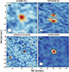 |
Fig. 1. [OI] 145μm emission maps. Contour lines correspond to [2, 3, 4, 5, 6, 8, 10, 15, 20, 30] σ confidence levels, where σ = 0.030, 0.098, 0.082 and 0.024 Jy beam−1 km s−1 for panels a, b, c, and d, respectively. In panel c, arrows indicate the location in which we detect [OI] or [CII] emission at z = 4.680, in addition to continuum emission (Figure B.1). In each panel, the bottom-left white ellipse shows the ALMA beam. |
We find [OI] 145μm luminosities in the range 2 × 10⁸ − 109 M⊙, that are a factor of about four to seven lower than the [CII] luminosities previously measured for these sources. Although some scatter might be due to the different sensitivities and beam sizes of the [CII] observations listed in Table 1, this result suggests that [OI] 145μm typically represents a significant fraction of the total [CII] luminosity. In J2054−0005 the [OI] 145μm luminosity corresponds to about 20% of that of [OI] 63μm and, similarly, [OI] 145μm/[OI] 63μm ≳ 25 \% for SPT0346−52.
Data for [OI] 145μm observations of A1689−zD1 from ALMA cycle 9 were presented in Fudamoto et al. (2025), with similar angular resolution and about two times lower sensitivity. We measure a consistent [OI] 145μm flux. Concerning SPT0346−52, we detect two bright sources in the [OI] map, the southern of which has an elongated, arc-like shape. We verified that this is consistent with the multiple images detected in high-resolution ALMA band 7 observations by Litke et al. (2019). Litke et al. (2022) reported a previous, low-S/N detection of [OI] 145μm in SPT0346−52, based on ALMA cycle 2 data with a ∼0.25 arcsec angular resolution, and evidence that this galaxy is undergoing a merger. We recover a factor of about four higher flux, likely because the low-resolution observation presented in this work better recovers the emission from diffuse gas dispersed by the merger.
At the ALMA resolution, we detected two distinct [OI] 145μm sources in the map of J204314−214439. They show a very similar [OI] line profile centered at the same redshift, which suggests that they are distinct images from the same galaxy, in agreement with the interpretation of this source by Zavala et al. (2015). Previous measurements of [CII] 158μm and IR luminosities in J204314−214439 were based on low resolution observations from SCUBA-2 (∼15 arcsec) and AzTEC/LMT (∼8 arcsec), respectively (Zavala et al. 2015). Accordingly, we created a new 0th moment map of [CII] emission based on ACA data from project 2021.1.00265.S (angular resolution 7.3 × 5.2 arcsec2, Figure B.1 left). As previous continuum observations have not allowed for robust disentanglement of the emission of two foreground galaxies along the line of sight from that of J204314−214439 (Zavala et al. 2015), we also used the 2023.1.01450.S data to create a high resolution map (0.75 × 0.65 arcsec2) of the ∼362.7 GHz continuum (Figure B.1 right). We find that the bulk of the continuum emission is located with an elongated source, likely associated with one of the foreground galaxies. Instead, we measure the continuum of J204314−214439 by considering only the emission from the multiple images in which we also detect [OI] and [CII] emission at z = 4.680. We derive the IR luminosity of J204314.2−214439 by fitting the ∼362.7 GHz continuum with a modified black body following the approach in Tripodi et al. (2024), by assuming a dust temperature of Td = 37 K and β = 1.70 (Zavala et al. 2015). These results are in line with the assumptions made in the simulation run (Maio et al. 2022).
3.2. Existing literature
We consider the compilation4 of Ramos Padilla et al. (2023) and references therein, including galaxies in a wide redshift range (0 ≤ z ≲ 6.5) with the detection of several FIR lines. Strong AGN galaxies are not present in this compilation.
We include the hot dust-obscured galaxy W2246–0526 at z = 4.601, with both [OI] 63μm and [OI] 145μm observations from Fernández Aranda et al. (2024), and a SFR estimated from the IR luminosity reported by Fan et al. (2018). We include the recent [OI] 63μm detection in the bright QSO J2054-0005 at z = 6.04 by Ishii et al. (2025). To date, this is the highest z detection of this line. We also consider the [OI] 145μm detection in the host galaxy of another luminous QSO J2310+1855 at z = 6.003 by Li et al. (2020). The upper limit of the z = 5.6 SPT0346−52 [OI] 63μm luminosity is taken from Litke et al. (2022). Finally, we include three main sequence star forming galaxies at 6.5 ≤ z ≤ 7.7 from the REBELS sample, for which [OI] 145μm were reported by Fudamoto et al. (2025).
4. Simulation results
In this section, we present the main results of our work concerning the modeled [OI] 63μm and [OI] 145μm luminosities of simulated galaxies. We do not present general simulation predictions – such as mass or UV luminosity functions, baryon fractions, galaxy main sequence, mass-metallicity relation, etc. – that have been discussed in previous works (Maio et al. 2022; Maio & Viel 2023; Casavecchia et al. 2024, 2025).
As an illustrative example of our modeling pipeline, in Fig. 2 we show the most massive galaxy (Mstars ∼ 3.5 × 10¹⁰ M⊙) in our simulation at z = 6.14, with gas particles color-coded by their [OI] 63μm and [OI] 145μm luminosities as well as their [OI] 63μm/[CII] 158μm and [OI] 145μm/[CII] 158μm ratios. From the ratios it can be inferred that [CII] 158μm emission that is extended and diffuse compared to the [OI] lines, which remain faint in the low-density (nH ≲ 102 cm−3) outer regions. In contrast, [OI] lines become significantly brighter in dense central regions (nH ≳ 104 cm−3Tgas ≲ 100 K), where their higher critical densities make them effective tracers of such conditions.
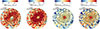 |
Fig. 2. Visualization of the [OI] 63μm and [OI] 145μm luminosities, and the [OI] 63μm/[CII] 158μm and [OI] 145μm/[CII] 158μm ratios, for the most massive simulated galaxy at z = 6.14. Black contours follow the gas density distribution. |
4.1. Predictions of [OI] 63μm self-absorption
The outcome of the simple model for [OI] 63μm self-absorption introduced in Sect. 2.2.3 is shown in Fig. 3, where the fraction of [OI] 63μm flux absorbed by foreground material is shown as a function of the SFR of our model galaxies at z = 6. We find no significant redshift evolution of this quantity in our model. The absorbed fraction increases with SFR, up to ∼ 1 M⊙/yr where it flattens and slowly decreases in the largest objects in our volume. The increasing trend of the relation is due to the major [OI] column density found in larger objects. At the same time, the flattening is due to the condition on velocities introduced in Eq. (4). Briefly, the velocity distribution of gas particles broadens faster than the velocity dispersion of GMCs with increasing SFR. As a consequence, at fixed column density, fewer particles in the line of sight can be targeted as absorbers. To prove this, we show in Fig. 3 what would be obtained without considering the Eq. (4) condition (no σv case) and in the rest of the paper we show results also for this version of the model to bracket our predictions.
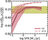 |
Fig. 3. Fraction of self-absorbed 63 μm [OI] line flux due to foreground material as a function of the galaxy SFR as predicted by our model. Solid lines refer to median trends while the shaded area are the 16th to 84th percentile dispersion. The solid line refers to the fiducial model, while the dashed one is obtained without considering the condition on velocity in Eq. (4). The yellow dashed region represent the typical values adopted in observational studies (reduction by a factor of two to four). |
Interestingly and despite its simplicity, for galaxies with SFR ≳0.1 M⊙/yr, our model yields attenuation factors that are broadly consistent with the empirically adopted corrections of two to four, as shown in Fig. 3. Nonetheless, we acknowledge the limitations of this approach. In particular, the absorbed radiation does not contribute to the excitation of the absorbing gas, which is assumed to be cold (Tex ≲ 50 K), such that only the ground state is significantly populated. A more rigorous treatment would involve solving the full radiative transfer problem iteratively, accounting for the mutual coupling between radiation and level populations in the absorbing material. However, this would be computationally prohibitive.
4.2. Luminosity functions
We began by examining the luminosity functions of [OI] 63μm and [OI] 145μm as predicted by our simulations at redshifts z = 6, 8, and 10. These are presented in Fig. 4, excluding data points below the low-luminosity threshold where sample incompleteness becomes relevant. Currently, observational determinations of these luminosity functions at such high redshifts are not available, and therefore, our predictions are intended to serve as theoretical benchmarks for future studies that will have sufficient data at z ≥ 6. The high-luminosity end of our predictions is well described by a simple power law, exhibiting a non-evolving slope of approximately −1.9 ± 0.1. The impact of [OI] 63μm self-absorption is very similar at all redshift, with a magnitude ≈3. The overall normalization increases with cosmic time, keeping track of the ongoing cosmological structure formation. This suggests an expected redshift evolution for the statistics of both OI lines already at such early epochs.
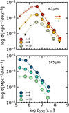 |
Fig. 4. Luminosity function of [OI] 63μm (top panel) and [OI] 145μm (bottom panel) at z = 6, 8, and 10 as predicted by our simulation. Errorbars are obtained by bootstrapping. The colored arrows in the top panel indicate the mean magnitude of the foreground self-absorption at each redshift. Low opacity points are those affected by resolution effects. |
4.3. Scaling relations
Here we present a set of scaling relations between the [OI] 63μm and [OI] 145μm line luminosities and various physical properties of our simulated galaxies at z = 6. The weak redshift evolution of these relations is discussed in Appendix C, while the predicted SFR–[CII] relation is in Appendix D.
Figure 5 shows the [OI] 63μm and [OI] 145μm line luminosities of our simulated galaxies as functions of stellar mass, gas-phase metallicity 12 + log(O/H), and H2 mass. We find a strong correlation between [OI] luminosities and both H2 mass and stellar mass. As for stellar mass, the relation flattens at the high end, where the star-forming gas becomes predominantly cold (T ≲ 50 K). Such a drop is particularly evident for the [OI] 145μm line. Unsurprisingly, the correlation with H2 mass is even tighter since both luminosities and H2 are derived by DESPOTIC. However, the [OI] 63μm−MH2 relation features a change of slope at MH2 ≈ 108 M⊙, due to the impact of foreground self-absorption, which becomes relevant at approximately these molecular masses, which are associated with SFR ≈ 1 M⊙/yr galaxies.
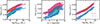 |
Fig. 5. Relations between the [OI] 63μm (red) and [OI] 145μm (blue) line luminosities and stellar mass (left), gas-phase metallicity traced by oxygen-to-hydrogen number ratio with respect to solar (middle), and H2 mass (right) for our simulated galaxies at z = 6. Solid lines represent the median trends, while density contours illustrate the underlying distribution of galaxies. |
In contrast, the relationship between [OI] 63μm and [OI] 145μm luminosities and gas-phase metallicity is considerably weaker, characterized by significant scatter. This increased dispersion is due to the implementation of metal production and diffusion in the simulation, which distributes metals among neighboring gas particles. While this approach is included to roughly account for unresolved sub-grid mixing processes, it also introduces additional scatter when analyzing metallicity at the resolution of individual gas particles. The sharp transition around 12 + log(O/H)≃8.2 marks the shift from galaxies dominated by warm gas (T ≳ 100 K) to those dominated by cold gas (T ≲ 100 K), leading to a reduction in [OI] emission per unit gas mass and hence a sharp flattening in the luminosity-metallicity relation.
The relation between [OI] 63μm and [OI] 145μm luminosities and galaxy SFR is shown in Fig. 6. Alongside our simulated results at z = 6, we include the results obtained from the post-processing of galaxy evolution simulations by Olsen et al. (2017) and Ramos Padilla et al. (2023). Various observational results are also presented (Sect. 3).
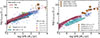 |
Fig. 6. Relation between [OI] 63μm (left panel) and [OI] 145μm (right panel) line luminosity and SFR. Our simulation results at z = 6 are shown as red density contours, with solid lines representing median trends. The median trend of the model with self-absorption neglecting the Eq. (4) condition is shown as a dashed line. Dotted lines are linear fits of the simulation results, with coefficients listed in Section 4.3. Other z ∼ 6 predictions for [OI] 63μm luminosity obtained from the post-processing of numerical simulations are also reported: Olsen et al. (2017) as blue circles and Ramos Padilla et al. (2023) as a turquoise area. Some observations are also reported for reference. The data up to z = 4 compiled by Ramos Padilla et al. (2023) are shown as hexagons. The J2054-00005 at z = 6.04 (Ishii et al. 2025) and W2246-0526 at z = 4.60 (Fernández Aranda et al. 2024) have both [OI] 63μm and [OI] 145μm detections. As for [OI] 145μm, we include the recent 6.5 ≤ z ≤ 7.7 REBELS observations (Fudamoto et al. 2025), the z = 6.00 J2310+1855 QSO (Li et al. 2020), and the new data obtained in this work (A1689-zD1 at z = 7.13, SPT0346−52 at z = 5.7 and J204313.2-214439 at z = 4.68; see Sect. 3). |
The relation between our predicted luminosities and SFR is quite tight, with a mild flattening at the high-SFR end, attributed to the colder gas in these galaxies. This flattening is particularly evident for [OI] 145μm, as its luminosity decreases more rapidly than that of [OI] 63μm with falling temperature. This is because the 3P0 level (from which the transition 3P0→3P1 originates) is hardly populated (as it requires ΔE/k ∼ 325 K). We find good agreement between our predictions and those of other theoretical studies, which is particularly remarkable considering the different post-processing techniques and simulations employed. Notably, our simulation is the only one that accounts for foreground absorption of [OI] 63μm emission by cold gas, which reduces the total line luminosity by a factor of approximately two to four (Fig. 3). The self-absorption model without the relative velocity condition (Eq. (4)) shows less agreement at high SFRs, where the effect is likely overestimated (≈90% of the flux is self-absorbed).
Due to the limited volume of our simulation, we cannot sample highly star-forming systems (≳100 M⊙/yr), which are predominantly the ones observed at high redshift. When comparing our extrapolated relations with observational data, we find good agreement, except for the W2246–0526 [OI] 63μm, which lies about an order of magnitude above our extrapolation. Note, however, the complex nature of this object, which is the most luminous galaxy in the Universe, likely hosting a heavily dust-obscured QSO (Díaz-Santos et al. 2016).
The extrapolation was obtained by fitting our results with the relation ![Mathematical equation: $ \log (L_\mathrm{{[OI]}} / L_\odot ) = a \, \log (\mathrm{{SFR}} / \mathrm{{M}_\odot \rm{yr}^{-1}}) + b $](/articles/aa/full_html/2026/01/aa57033-25/aa57033-25-eq8.gif) , with coefficients
, with coefficients ![Mathematical equation: $ (a_{{\mathrm{{[OI]}}\, 63 {{\upmu}\rm{m}}}}, b_{{\mathrm{{[OI]}}\, 63 {{\upmu}\rm{m}}}}) = (0.76, 7.11) $](/articles/aa/full_html/2026/01/aa57033-25/aa57033-25-eq9.gif) and
and ![Mathematical equation: $ (a_{{{\rm{[OI]}}\, 145 {{\upmu}\rm{m}}}}, b_{{{\rm{[OI]}}\, 145 {{\upmu}\rm{m}}}}) = (0.89, 6.40) $](/articles/aa/full_html/2026/01/aa57033-25/aa57033-25-eq10.gif) for [OI] 63μm and [OI] 145μm, respectively. The scatter of the relation is ≈0.5 dex for both lines and almost SFR independent.
for [OI] 63μm and [OI] 145μm, respectively. The scatter of the relation is ≈0.5 dex for both lines and almost SFR independent.
4.4. Line ratios
In Fig. 7 we report our model predictions for line ratios at z = 6 (i.e., [OI] 63μm/[CII] 158μm, [OI] 145μm/[CII] 158μm and [OI] 145μm/[OI] 63μm) and compare them with available observations. We note that the [OI] 63μm/[CII] 158μm and [OI] 145μm/[CII] 158μm ratios increase by a factor of two to three at higher redshifts, whereas the [OI] 145μm/[OI] 63μm ratio shows little redshift evolution (see Appendix C for details). We note that our simulation probes normal star forming galaxies with SFRs up to ≈ 100 M⊙/yr, generally below the SFRs of powerful high-z observed sources. Therefore, extrapolations above those values must be taken with caution.
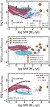 |
Fig. 7. Line ratios as a function of SFR: [OI] 63μm/[CII] 158μm (top), [OI] 145μm/[CII] 158μm (middle) and [OI] 145μm/[OI] 63μm (bottom). Our simulation results at z = 6 are shown with red contours, with the solid line representing median trend. The median trend of the model with self-absorption neglecting the Eq. (4) condition is shown as a dashed line. The black arrows indicate the magnitude of the [OI] 63μm self-absorption by foreground gas as predicted by our model. Simulation predictions by Ramos Padilla et al. (2023) at z ∼ 6 are shown as turquoise contours. The same observational data shown in Fig. 6 are included where detections are available, as described in the legend. |
4.4.1. [OI] 63μm/[CII] 158μm
The top panel of Fig. 7 shows the [OI] 63μm/[CII] 158μm ratio. Our model predicts a ratio of ≈1, slightly increasing at both low and high SFR (up to ≈2). The low SFR end increase is due to the lower contribution of foreground [OI] 63μm self-absorption, while the high end one is mainly driven by the flattening of the [CII] 158μm−SFR relation (Appendix D). Observations suggest a z−independent ratio close to 1, with a factor of ≈2 scatter. The ratio measured for J2054-0005 is consistent with our values, whereas W2246-0526 is somewhat higher; however, both objects have SFRs significantly above those of our simulated galaxies. Our results incorporate the effect of [OI] 63μm self-absorption by cold foreground gas. Without this contribution, the [OI] 63μm/[CII] 158μm ratio would be a factor of ≈2 higher, slightly overestimating the observational data. We note that the simulations-based ratios reported by Ramos Padilla et al. (2023), where this effect is not taken into account, are indeed slightly larger than ours.
Finally, we note that the self-absorption model without the condition of Eq. (4) yields ratios well below the observed high-z values (with the exception of the SPT0346-52 upper limit). Interestingly, De Breuck et al. (in prep.) report [OI] 63μm/[CII] 158μm ratios reaching ≲0.01 in a sample of 12 SPT high−z dusty star-forming galaxies, suggesting a stronger role of self-absorption and leaving room for possible refinements of this modeling in the high-SFR regime.
4.4.2. [OI] 145μm/[CII] 158μm
The [OI] 145μm/[CII] 158μm ratio offers a potential advantage over the [OI] 63μm/[CII] 158μm ratio, as the 145 μm oxygen line is optically thin and thus not affected by uncertainties from foreground self-absorption. Moreover, this ratio is particularly useful in observations for inferring gas densities (Peng et al. 2025b). We include recent results from Fudamoto et al. (2025) for z ∼ 7 REBELS galaxies and the z = 6.00 QSO J2310+1855 (Ishii et al. 2025), along with new observations from this work presented in Sect. 3.1, which nearly double the number of available data points for this ratio at such high redshift.
Our model predicts a constant [OI] 145μm/[CII] 158μm value of ≈0.15 with a scatter of a factor ≲2 (Fig. 7, central panel). Our estimates are a factor of ≈2 higher than those presented by Ramos Padilla et al. (2023). Despite the large scatter, observations at z ≳ 5 show [OI] 145μm/[CII] 158μm ratios ranging from 0.08 to 0.4. Although simulated SFRs do not exactly overlap with the observed SFR range, observed ratios are fully consistent with our simulation values. No significant variation is found among the QSOs in the sample.
4.4.3. [OI] 145μm/[OI] 63μm
The [OI] 145μm/[OI] 63μm ratio is a great indicator of the self-absorption of [OI] 63μm, since the two lines have similar critical densities and [OI] 145μm being optically thin. Without self-absorption effects, this ratio is expected to be ≲0.1 for gas with typical physical ISM conditions (see discussion in Sect. 5.1). Due to self-absorption, our model galaxies feature a [OI] 145μm/[OI] 63μm ratio of ≈0.25 − 0.1, instead of being a factor of two to four lower (Fig. 7, bottom panel). The ratio features a decrease at both low and high SFRs, respectively due to the lower impact of [OI] 63μm and the high-SFR flattening of the [OI] 145μm−SFR relation. Note that the self-absorption factor is approximately the gap with Ramos Padilla et al. (2023) predictions, which do not account for this effect. Our model predicts slightly higher values than observed at z ≲ 0.5, but yields ratios consistent with the only detections currently available at z ≳ 4.6 (J2024-0005 and W2246-0526). Instead, when using the self-absorption model that neglects the condition in Eq. (4), values up to ≈1 are obtained in the high-SFR regime.
5. Discussion
5.1. Foreground [OI] 63μm self-absorption
Our results highlight the relevance of cold foreground self-absorption of the [OI] 63μm line. This reduces the observed intensity by a factor of two to four, which is consistent with the approach adopted by various observational works. However, being this value very uncertain studying the ratio between [OI] 63μm and other optically thin lines ([OI] 145μm, [CII] 158μm) becomes essential to investigate the impact of self-absorption. Our results, together with the observations available (Fig. 7, central panel), indicate a [OI] 145μm/[CII] 158μm ratio of ≈0.1–0.6. We conduct a set of experiments with DESPOTIC to see which are the values of [OI] 145μm/[OI] 63μm and [OI] 63μm/[CII] 158μm expected to be consistent with the above ratio. In these experiments, we assume homogeneous clouds and the standard GOW chemical network (Sect. 2.2), letting the gas density and temperature varying in the range nH ∈ [102, 106] cm−3 and T ∈ [20, 104] K. A radius of 10 pc is assumed to convert the volume density to column density. Results of this experiments are shown in Fig. 8 as a region colored according to the [OI] 145μm/[CII] 158μm ratio. In the same figure we also report our simulated galaxies together with J2054-0005, W2246-0526 and SPT0346−52 (limits). The typical densities and temperatures needed to produce the observed ratio of [OI] 145μm/[CII] 158μm would also produce a [OI] 63μm/[CII] 158μm and [OI] 145μm/[OI] 63μm ratios of, respectively, ≈2 − 10 and ≲0.1. These values differ by a factor of about two from those measured in J2054-0005. A similar, or even larger, discrepancy is suggested by the upper limits of SPT0346−52. In contrast, W2246–0546 is closer to these values.
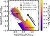 |
Fig. 8. Distribution of the [OI] 145μm/[OI] 63μm and [OI] 63μm/[CII] 158μm line ratios for different values of [OI] 145μm/[CII] 158μm, as shown in the colorbar. The colored region represents the outcome of the PDR DESPOTIC computations assuming homogeneous clouds with 102 ≤ nH/cm−3 ≤ 106 and 20 ≤ T/K ≤ 104. Our simulated z ≃ 6 galaxies are shown as circles, J2054-0005 as a star, W2246-0526 as a plus and the SPT0346−52 upper limit as a diamond. The black arrow illustrates the typical shift due to [OI] 63μm foreground self-absorption. |
Our simulated galaxies – for which foreground [OI] 63μm self-absorption is taken into account – are instead more in line with observations. This simple yet motivated reasoning highlights the need of [OI] 63μm observations (or even non-detections) of targets with known [OI] 145μm and [CII] 158μm fluxes, which would constrain the foreground self-absorption at such high z.
We conclude by noting that Peng et al. (2025a), who recently compiled an extensive dataset of FIR emission lines across a wide redshift range, also highlighted challenges in reproducing the observed [OI] 145μm/[OI] 63μm and [OI] 145μm/[CII] 158μm line ratios with theoretical models. They suggested that [OI] 63μm self-absorption could be a significant factor contributing to these discrepancies.
5.2. Mass-to-light ratios MH2/L[OI]
We discuss our z = 6 model predictions for the mass-to-light ratio MH2/L[OI] as a function of SFR and compare them with the observations available in Fig. 9. Our simulated galaxies feature a slowly increasing MH2/L[OI] − SFR relation at SFR ≳ 0.3 M⊙/yr, and the slope is similar for the two lines. Below this threshold, the ratio rapidly increases, due to the scarcity of molecular mass in galaxies with typically low column densities (NH ≲ 1022 cm−2). Excluding these points, we fit our results with a simple linear relation of the form ![Mathematical equation: $ \log \left( \frac{L_\mathrm{{[OI]}}}{M_{\mathrm{H_2}}} \cdot \frac{M_\odot}{L_\odot} \right) = a \cdot \log \left( \frac{\mathrm{{SFR}}}{M_\odot,\mathrm{{yr}}^{-1}} \right) + b $](/articles/aa/full_html/2026/01/aa57033-25/aa57033-25-eq11.gif) , with the resulting coefficients listed in Table 2, along with those obtained from fits as a function of metallicity and stellar mass.
, with the resulting coefficients listed in Table 2, along with those obtained from fits as a function of metallicity and stellar mass.
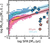 |
Fig. 9. Mass-to-light ratio MH2/L[OI] for [OI] 63μm and [OI] 145μm, respectively in red and blue color scales. We report simulation predictions at z = 6 (contours) and linear fits for log(SFR/M⊙yr−1) ≥ −0.5. Observational results (Sect. 3) for REBELS galaxies (pentagons), A1689-zD1 (hexagon), J204313.2-214439 (diamond), SPT0346−52 (small diamond), W2246-0526 (plus), J2054-0005 (star), and J2310+1855 (cross) are also reported. |
Best-fitting parameters of the mass-to-light ratio as a function of physical quantities.
Two main factors drive the slow increase in the mass-to-light ratio observed in all three cases. First, the gas in star-forming, massive, and metal-rich galaxies tends to be colder, which lowers the specific luminosity of emission lines. Second, the higher metallicity – associated with increased dust content in our post-processing model – combined with the high column densities typical of more massive galaxies, creates optimal conditions for H2 formation.
Our model well reproduces the ≈0.003 − 0.01 ![Mathematical equation: $ L_{{{\rm{[OI]}}\, 145 {{\upmu}\rm{m}}}}/M_{\mathrm{H_2}} $](/articles/aa/full_html/2026/01/aa57033-25/aa57033-25-eq12.gif) ratio featured by the REBELS galaxies and A1689-zD1, although these have a larger scatter than our tight relation. Instead, when comparing to the bright SMGs (SFR ≳ 1000 M⊙/yr) and QSOs, our predictions are above observationally derived ratios up to one order of magnitude, for both the [OI] 63μm and [OI] 145μm line. This implies typical lower mass-to-light ratios for the SMG and QSO population, as already noticed for the [CII] 158μm line (Salvestrini et al. 2025), and in general for highly star forming galaxies (Rizzo et al. 2020, 2021).
ratio featured by the REBELS galaxies and A1689-zD1, although these have a larger scatter than our tight relation. Instead, when comparing to the bright SMGs (SFR ≳ 1000 M⊙/yr) and QSOs, our predictions are above observationally derived ratios up to one order of magnitude, for both the [OI] 63μm and [OI] 145μm line. This implies typical lower mass-to-light ratios for the SMG and QSO population, as already noticed for the [CII] 158μm line (Salvestrini et al. 2025), and in general for highly star forming galaxies (Rizzo et al. 2020, 2021).
Finally, we note that although the H2 abundance predicted by the simulation is used within the star formation model, in this work we refer to molecular gas masses derived using DESPOTIC. The inferred estimates are valid for sub-grid unresolved scales and are typically larger by ∼1 dex compared to the on-the-fly values obtained for resolved scales. We choose to adopt the post-process values, because they are discussed in the context of line luminosities, which are also computed in post-processing and account for sub-resolution structures at densities higher than those resolved in the simulation.
5.3. Model variations
In this section, we present a series of numerical tests using different DESPOTIC configurations to assess the sensitivity of our results to key model assumptions. Specifically, we examine the impact of varying the CR heating prescription and the internal density profile of molecular clouds. Figure 10 shows the resulting [OI] 145μm luminosities and [OI] 145μm/[CII] 158μm ratios as functions of the SFR for our z = 6 model galaxies under different parameter choices. Although we focus here on a subset of lines, we checked that similar trends are observed also in other emission lines and ratios.
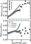 |
Fig. 10. [OI] 145μm luminosity and [OI] 145μm/[CII] 158μm ratio as a function of SFR for our model galaxies at z = 6. Different colors refer to different model assumptions in the post-processing pipeline with DESPOTIC. The red one represents the fiducial model adopted in this work, the cyan is a model where the CRs rate is scaled with the SFR density, the yellow and purple are models where the density profile is assumed to be logotropic and power-law. Solid lines refer to median trends and shaded regions indicate the 16th to 84th percentile dispersion. For reference, the available z ≳ 5 observations discussed in this work are also reported, with the same symbols as in Figs. 6 and 7. |
We begin by examining the impact of varying the cloud density profiles. Adopting either a logotropic or power-law profile (Popping et al. 2019) – both commonly used in the literature (e.g., Olsen et al. 2017; Garcia et al. 2024; Khatri et al. 2025) – results in only minor changes to the predicted emission. This finding confirms the results of Popping et al. (2019), who explored variations in density profiles and other sub-resolution cloud properties. The limited impact is essentially due to the fact that both the logotropic and power-law profiles converge toward the average density in the outer regions of the clouds, which dominate the emission due to their higher temperatures. As a result, the total line luminosities remain largely unaffected.
Next, we modify the CR heating model in DESPOTIC by implementing a scaling with the (unattenuated) SFR density, i.e.,  . This prescription is widely adopted in the literature (e.g., Popping et al. 2019; Garcia et al. 2024). As anticipated by the work of Krumholz et al. (2023), which motivates our CRs treatment, this SFR-based scaling leads to CRs energy densities also 2 − 3 orders of magnitude higher in the most massive galaxies compared to our fiducial model. Consequently, the gas in GMCs becomes significantly warmer, with typical temperatures around Tgas ≈ 100 K, compared to ≈30 K in the fiducial case. This increased heating boosts line emission in strongly star-forming systems and prevents the suppression of [CII] 158μm and [OI] 145μm luminosities. However, while this improves agreement with observed line luminosities, it leads to [OI] 145μm/[CII] 158μm and [OI] 63μm/[CII] 158μm ratios that are too high, typically exceeding the observed values of ≈1 and ≈0.3 dex, respectively.
One possible explanation for this discrepancy might be a missing contribution to [CII] 158μm emission from warm/hot ionized gas. At temperatures T ≳ 104 K, oxygen is expected to be ionized, while carbon can remain singly ionized up to a few 104 K. To account for this, we include a [CII] 158μm contribution from warm, non-star-forming gas particles by using the density and temperature predicted by our hydrodynamic simulation. We restrict this analysis to particles with T ≤ 105 K, under the (optimistic) assumption that CIII dominates at higher temperatures. The resulting contribution is negligible, though, and typically accounts for only ≈0.01 − 0.1 of the total [CII] 158μm luminosity, due to the low densities involved (nH ≲ 1 cm−3). To test whether this result is resolution-limited, we also model the density of the warm/hot gas as a log-normal distribution. However, this yields similar results, confirming the limited role of hot-phase [CII] 158μm emission.
5.4. Comparison with literature
We briefly discuss our results in the context of previous simulations and observations, as well as the new observations analyzed in this study.
Previous hydrodynamical simulations at z ≃ 6 (e.g., Olsen et al. 2017; Ramos Padilla et al. 2023), have attempted to model [OI] lines and ratios with more simplified treatments. A key difference lies in our inclusion of [OI] 63μm self-absorption due to foreground gas, a physical effect that has not been accounted for in other works. Although [OI] 63μm luminosities in Ramos Padilla et al. (2023) are comparable to ours, their [OI] 145μm/[CII] 158μm ratios are systematically lower. This suggests that their model underestimates the intrinsic emission strength of both [OI] lines. We point out that, instead, our inclusion of self-absorption allows our model to better reproduce the full set of observed ratios.
A comparison of our predictions with both the new data presented here and the observations available in the literature (Ishii et al. 2025; Fudamoto et al. 2025; Li et al. 2020) reveals broadly consistent trends in [OI] 63μm, [OI] 145μm, and [CII] 158μm line luminosities as a function of SFR. The high-z observations typically span a higher SFR regime than that covered by our simulations. Predicted and observed ratios among different line tracers are also consistent. These data, together with the compilation by Ramos Padilla et al. (2023), do not show a strong dependence of these quantities on redshift. This supports the idea of weak or negligible evolution in the luminosity–SFR relation and line ratios, in agreement with our findings over 6 ≤ z ≤ 10. We remark that the high-z observations typically span a higher SFR regime than that covered by our simulations. Deeper observations of z ≈ 6 targets with SFRs ≲ 100 M⊙ yr−1 are challenging with current facilities, as this would require exposure times of several hours per galaxy. Alternatively, applying a post-processing pipeline such as the one presented here may enable comparisons with high-z systems in large-volume cosmological simulations – for example MillenniumTNG (Pakmor et al. 2023); Magneticum Pathfinder (Dolag et al. 2025); COLIBRE (Schaye et al. 2025) – which can host galaxies with SFRs up to ≈ 103 M⊙ yr−1 at z ≈ 6.
While in this work we focus on simulated star formation–powered systems, the radiative contribution from AGNs may play a role in the resulting line emission. Previous studies reported higher [OI] 63μm/[CII] 158μm ratios in AGN-dominated systems due to the enhanced cooling efficiency of [OI] 63μm in warm, dense gas (Herrera-Camus et al. 2018) or the highly ionizing radiation from AGNs (Li et al. 2020). This is also consistent with the [CII] 158μm/FIR deficit observed in AGNs (e.g., Venemans et al. 2020).
Finally, in the three lensed galaxies and one QSO host galaxy at z ≳ 4.7 analyzed in this work, we measure [OI] 145μm luminosities ≳2 × 10⁸ L⊙. These values are at the bright end of the ones previously reported by Novak et al. (2019) and Fudamoto et al. (2025) and make these sources among the largest molecular-gas reservoirs at these epochs (Table 1).
6. Conclusions
In this paper, we performed theoretical predictions for the line emission of atomic neutral oxygen ([OI] 63μm and [OI] 145μm) in high-redshift galaxies. We exploited the COLDSIM cosmological hydrodynamic simulations post-processed with the radiative transfer code DESPOTIC to model the chemical, thermal, and statistical state of sub-resolution ISM clouds and compute the resulting line luminosities. For the first time, our pipeline includes a physically motivated model for [OI] 63μm self-absorption by cold foreground gas, an effect often neglected in previous theoretical works. We have also presented new ALMA measurements of [OI] 145μm emission in four objects at z ≳ 5.
Our main findings can be summarized as follows.
-
We find strong correlations between SFR and [OI] 63μm or [OI] 145μm luminosities, while diagnostic line ratios, such as [OI] 63μm/[CII] 158μm, [OI] 145μm/[CII] 158μm, and [OI] 145μm/[OI] 63μm, are nearly independent of SFR. These relations show minimal evolution over 6 ≤ z ≤ 10.
-
ALMA observations of [OI] 145μm show luminosities in the range ∼108–109 L⊙, a factor ∼4–7 lower than [CII] luminosities, and inferred ratios [OI] 145μm/[OI] 63μm ≳ 0.2.
-
Our model of [OI] 63μm self-absorption shows that intrinsic [OI] 63μm luminosities are about 2-4 times higher than what is actually observed and modeling self-absorption is essential to reproduce the observed line ratios successfully.
-
The [OI] 63μm and [OI] 145μm lines are both good tracers of molecular gas in normal star forming galaxies, and this makes them valuable alternatives to traditional tracers such as CO, which is affected by the cosmic microwave background at high z (da Cunha et al. 2013). Current measurements of MH2-to-L{OI] ratios in highly star forming galaxies and QSOs fall below our predictions, possibly indicating a deficit of molecular content, different ISM conditions, or extreme excitation mechanisms in those environments (Bischetti et al. 2021; Circosta et al. 2021).
This work is relevant for the relatively new subject of self-absorbed high-z fine-structure lines and establishes a path for further scientific developments in the field. Our results, in keeping with observations, offer robust predictions for future detections and support the use of [OI] lines as tracers of star formation activity and molecular gas in the early Universe. Despite the effects of self-absorption, the [OI] 63μm line remains as bright as, or even brighter than, the [CII] 158μm line. However, its detectability at z ≳ 6 is limited by atmospheric opacity in ALMA Bands 8–10. In contrast, the lower optical depth of the [OI] 145μm line makes it more accessible to ALMA, as indicated by the high luminosities measured for the four high-z galaxies considered in this work. Upcoming ALMA observations targeting the two [OI] lines discussed here will provide valuable constraints on the physical conditions of the ISM and the role of [OI] 63μm self-absorption during the epoch of reionization.
Derived assuming particles are spheres of volume Vpart = Mpart/ρpart, with ρpart simulated particle density.
We have checked that this number is sufficient to reach convergence.
Available at https://zenodo.org/records/6576202.
Acknowledgments
We thank the referee for the useful suggestions which improved this manuscript. MP acknowledges useful discussions with D. Narayanan, K. Garcia, and D. Valentin-Martinez, and thanks the organizers of the Infrared Fine-Structure Lines Workshop 2025 at Winona State University. This paper makes use of the following ALMA data: ADS/JAO.ALMA#2023.1.01450.S (P.I. C. Ferkinhoff) and ADS/JAO.ALMA#2021.1.00265.S (P.I. D. Riechers). ALMA is a partnership of ESO (representing its member states), NSF (USA), and NINS (Japan), together with NRC (Canada), MOST and ASIAA (Taiwan), and KASI (Republic of Korea), in cooperation with the Republic of Chile. The Joint ALMA Observatory is operated by ESO, AUI/NRAO and NAOJ. UM and MP acknowledge financial support from grant no. 1.05.23.06.13 “FIRST – First Galaxies in the Cosmic Dawn and the Epoch of Reionization with High Resolution Numerical Simulations”, awarded by the Italian National Institute of Astrophysics (INAF). UM also acknowledges financial support from INAF travel grant no. 1.05.23.04.01. CR and GLG acknowledge financial support from the European Union’s HORIZON-MSCA-2021-SE-01 Research and Innovation Programme under the Marie Sklodowska-Curie grant agreement number 101086388 – Project (LACEGAL). CF, FS and MB acknowledge financial support from Ricerca Fondamentale INAF 2023 Data Analysis grant 1.05.23.03.04 “ARCHIE ARchive Cosmic HI & ISM Evolution”. FS and MB acknowledge financial support from the PRIN MUR 2022 2022TKPB2P - BIG-z, Ricerca Fondamentale INAF 2024 under project 1.05.24.07.01 MINI-GRANTS RSN1 “ECHOS”, Bando Finanziamento ASI CI-UCO-DSR-2022-43 CUP:C93C25004260005 project “IBISCO: feedback and obscuration in local AGN”.
References
- Abel, T., Anninos, P., Zhang, Y., & Norman, M. L. 1997, New A, 2, 181 [NASA ADS] [CrossRef] [Google Scholar]
- Akins, H. B., Fujimoto, S., Finlator, K., et al. 2022, ApJ, 934, 64 [NASA ADS] [CrossRef] [Google Scholar]
- Apostolovski, Y., Aravena, M., Anguita, T., et al. 2019, A&A, 628, A23 [NASA ADS] [CrossRef] [EDP Sciences] [Google Scholar]
- Bayet, E., Williams, D. A., Hartquist, T. W., & Viti, S. 2011, MNRAS, 414, 1583 [NASA ADS] [CrossRef] [Google Scholar]
- Bischetti, M., Feruglio, C., Piconcelli, E., et al. 2021, A&A, 645, A33 [NASA ADS] [CrossRef] [EDP Sciences] [Google Scholar]
- Bonatto, C., & Bica, E. 2011, MNRAS, 415, 2827 [NASA ADS] [CrossRef] [Google Scholar]
- Brisbin, D., Ferkinhoff, C., Nikola, T., et al. 2015, ApJ, 799, 13 [Google Scholar]
- Casavecchia, B., Maio, U., Péroux, C., & Ciardi, B. 2024, A&A, 689, A106 [NASA ADS] [CrossRef] [EDP Sciences] [Google Scholar]
- Casavecchia, B., Maio, U., Péroux, C., & Ciardi, B. 2025, A&A, 693, A119 [NASA ADS] [CrossRef] [EDP Sciences] [Google Scholar]
- Caux, E., Ceccarelli, C., Castets, A., et al. 1999, A&A, 347, L1 [NASA ADS] [Google Scholar]
- Circosta, C., Mainieri, V., Lamperti, I., et al. 2021, A&A, 646, A96 [EDP Sciences] [Google Scholar]
- Coppin, K. E. K., Danielson, A. L. R., Geach, J. E., et al. 2012, MNRAS, 427, 520 [NASA ADS] [CrossRef] [Google Scholar]
- da Cunha, E., Groves, B., Walter, F., et al. 2013, ApJ, 766, 13 [Google Scholar]
- De Breuck, C., Weiß, A., Béthermin, M., et al. 2019, A&A, 631, A167 [NASA ADS] [CrossRef] [EDP Sciences] [Google Scholar]
- De Looze, I., Cormier, D., Lebouteiller, V., et al. 2014, A&A, 568, A62 [NASA ADS] [CrossRef] [EDP Sciences] [Google Scholar]
- Decarli, R., & Díaz-Santos, T. 2025, A&ARv, 33, 4 [Google Scholar]
- Díaz-Santos, T., Assef, R. J., Blain, A. W., et al. 2016, ApJ, 816, L6 [Google Scholar]
- Díaz-Santos, T., Armus, L., Charmandaris, V., et al. 2017, ApJ, 846, 32 [Google Scholar]
- Dolag, K., Borgani, S., Murante, G., & Springel, V. 2009, MNRAS, 399, 497 [Google Scholar]
- Dolag, K., Remus, R. S., Valenzuela, L. M., et al. 2025, arXiv e-prints [arXiv:2504.01061] [Google Scholar]
- Draine, B. T. 2011, Physics of the Interstellar and Intergalactic Medium (Princeton University Press) [Google Scholar]
- Fan, L., Gao, Y., Knudsen, K. K., & Shu, X. 2018, ApJ, 854, 157 [NASA ADS] [CrossRef] [Google Scholar]
- Farrah, D., Lebouteiller, V., Spoon, H. W. W., et al. 2013, ApJ, 776, 38 [Google Scholar]
- Ferland, G. J., Chatzikos, M., Guzmán, F., et al. 2017, Rev. Mex. Astron. Astrofis., 53, 385 [NASA ADS] [Google Scholar]
- Fernández Aranda, R., Díaz Santos, T., Hatziminaoglou, E., et al. 2024, A&A, 682, A166 [NASA ADS] [CrossRef] [EDP Sciences] [Google Scholar]
- Fernández-Ontiveros, J. A., Spinoglio, L., Pereira-Santaella, M., et al. 2016, ApJS, 226, 19 [CrossRef] [Google Scholar]
- Ferrara, A., Sommovigo, L., Dayal, P., et al. 2022, MNRAS, 512, 58 [NASA ADS] [CrossRef] [Google Scholar]
- Fudamoto, Y., Inoue, A. K., Bouwens, R., et al. 2025, arXiv e-prints [arXiv:2504.03831] [Google Scholar]
- Garcia, K., Narayanan, D., Popping, G., et al. 2024, ApJ, 974, 197 [NASA ADS] [CrossRef] [Google Scholar]
- Gerin, M., Ruaud, M., Goicoechea, J. R., et al. 2015, A&A, 573, A30 [NASA ADS] [CrossRef] [EDP Sciences] [Google Scholar]
- Glover, S. C. O., & Clark, P. C. 2012, MNRAS, 426, 377 [Google Scholar]
- Glover, S. C. O., & Mac Low, M.-M. 2007, ApJS, 169, 239 [NASA ADS] [CrossRef] [Google Scholar]
- Goldsmith, P. F. 2019, ApJ, 887, 54 [NASA ADS] [CrossRef] [Google Scholar]
- Goldsmith, P. F., Langer, W. D., Seo, Y., et al. 2021, ApJ, 916, 6 [NASA ADS] [CrossRef] [Google Scholar]
- Gong, M., Ostriker, E. C., & Wolfire, M. G. 2017, ApJ, 843, 38 [NASA ADS] [CrossRef] [Google Scholar]
- Hernandez-Monteagudo, C., Maio, U., Ciardi, B., & Sunyaev, R. A. 2017, arXiv e-prints [arXiv:1707.01910] [Google Scholar]
- Herrera-Camus, R., Sturm, E., Graciá-Carpio, J., et al. 2018, ApJ, 861, 94 [Google Scholar]
- Herrera-Camus, R., González-López, J., Förster Schreiber, N., et al. 2025, A&A, 699, A80 [NASA ADS] [CrossRef] [EDP Sciences] [Google Scholar]
- Ishii, N., Hashimoto, T., Ferkinhoff, C., et al. 2025, PASJ, 77, 139 [NASA ADS] [CrossRef] [Google Scholar]
- Katz, H., Galligan, T. P., Kimm, T., et al. 2019, MNRAS, 487, 5902 [NASA ADS] [CrossRef] [Google Scholar]
- Kennicutt, R. C., & Evans, N. J. 2012, ARA&A, 50, 531 [NASA ADS] [CrossRef] [Google Scholar]
- Khatri, P., Porciani, C., Romano-Díaz, E., Seifried, D., & Schäbe, A. 2024, A&A, 688, A194 [NASA ADS] [CrossRef] [EDP Sciences] [Google Scholar]
- Khatri, P., Romano-Díaz, E., & Porciani, C. 2025, A&A, 697, A174 [NASA ADS] [CrossRef] [EDP Sciences] [Google Scholar]
- Killi, M., Watson, D., Fujimoto, S., et al. 2023, MNRAS, 521, 2526 [NASA ADS] [CrossRef] [Google Scholar]
- Krumholz, M. R. 2014, MNRAS, 437, 1662 [NASA ADS] [CrossRef] [Google Scholar]
- Krumholz, M. R., Crocker, R. M., & Offner, S. S. R. 2023, MNRAS, 520, 5126 [NASA ADS] [CrossRef] [Google Scholar]
- Lagache, G., Cousin, M., & Chatzikos, M. 2018, A&A, 609, A130 [NASA ADS] [CrossRef] [EDP Sciences] [Google Scholar]
- Lagos, C. d. P., Bayet, E., Baugh, C. M., et al. 2012, MNRAS, 426, 2142 [NASA ADS] [CrossRef] [Google Scholar]
- Leurini, S., Wyrowski, F., Wiesemeyer, H., et al. 2015, A&A, 584, A70 [NASA ADS] [CrossRef] [EDP Sciences] [Google Scholar]
- Li, J., Wang, R., Cox, P., et al. 2020, ApJ, 900, 131 [NASA ADS] [CrossRef] [Google Scholar]
- Litke, K. C., Marrone, D. P., Spilker, J. S., et al. 2019, ApJ, 870, 80 [Google Scholar]
- Litke, K. C., Marrone, D. P., Aravena, M., et al. 2022, ApJ, 928, 179 [NASA ADS] [CrossRef] [Google Scholar]
- Lupi, A., Pallottini, A., Ferrara, A., et al. 2020, MNRAS, 496, 5160 [Google Scholar]
- Ma, J., Gonzalez, A. H., Spilker, J. S., et al. 2015, ApJ, 812, 88 [NASA ADS] [CrossRef] [Google Scholar]
- Maio, U., & Viel, M. 2023, A&A, 672, A71 [NASA ADS] [CrossRef] [EDP Sciences] [Google Scholar]
- Maio, U., Dolag, K., Ciardi, B., & Tornatore, L. 2007, MNRAS, 379, 963 [NASA ADS] [CrossRef] [Google Scholar]
- Maio, U., Ciardi, B., Yoshida, N., Dolag, K., & Tornatore, L. 2009, A&A, 503, 25 [NASA ADS] [CrossRef] [EDP Sciences] [Google Scholar]
- Maio, U., Ciardi, B., Dolag, K., Tornatore, L., & Khochfar, S. 2010, MNRAS, 407, 1003 [CrossRef] [Google Scholar]
- Maio, U., Khochfar, S., Johnson, J. L., & Ciardi, B. 2011, MNRAS, 414, 1145 [NASA ADS] [CrossRef] [Google Scholar]
- Maio, U., Péroux, C., & Ciardi, B. 2022, A&A, 657, A47 [NASA ADS] [CrossRef] [EDP Sciences] [Google Scholar]
- Malhotra, S., Kaufman, M. J., Hollenbach, D., et al. 2001, ApJ, 561, 766 [Google Scholar]
- Narayanan, D., & Krumholz, M. R. 2017, MNRAS, 467, 50 [NASA ADS] [CrossRef] [Google Scholar]
- Nelson, R. P., & Langer, W. D. 1999, ApJ, 524, 923 [NASA ADS] [CrossRef] [Google Scholar]
- Novak, M., Bañados, E., Decarli, R., et al. 2019, ApJ, 881, 63 [NASA ADS] [CrossRef] [Google Scholar]
- Olsen, K. P., Greve, T. R., Narayanan, D., et al. 2015, ApJ, 814, 76 [CrossRef] [Google Scholar]
- Olsen, K., Greve, T. R., Narayanan, D., et al. 2017, ApJ, 846, 105 [Google Scholar]
- Pakmor, R., Springel, V., Coles, J. P., et al. 2023, MNRAS, 524, 2539 [NASA ADS] [CrossRef] [Google Scholar]
- Pallottini, A., Ferrara, A., Gallerani, S., et al. 2017, MNRAS, 465, 2540 [CrossRef] [Google Scholar]
- Pallottini, A., Ferrara, A., Gallerani, S., et al. 2022, MNRAS, 513, 5621 [NASA ADS] [Google Scholar]
- Peng, B., Lamarche, C., Ball, C., et al. 2025a, arXiv e-prints [arXiv:2507.10702] [Google Scholar]
- Peng, B., Vishwas, A., Lamarche, C., et al. 2025b, arXiv e-prints [arXiv:2507.11829] [Google Scholar]
- Poglitsch, A., Herrmann, F., Genzel, R., et al. 1996, ApJ, 462, L43 [NASA ADS] [CrossRef] [Google Scholar]
- Popping, G., & Péroux, C. 2022, MNRAS, 513, 1531 [CrossRef] [Google Scholar]
- Popping, G., Narayanan, D., Somerville, R. S., Faisst, A. L., & Krumholz, M. R. 2019, MNRAS, 482, 4906 [Google Scholar]
- Ramos Padilla, A. F., Wang, L., van der Tak, F. F. S., & Trager, S. C. 2023, A&A, 679, A131 [NASA ADS] [CrossRef] [EDP Sciences] [Google Scholar]
- Rizzo, F., Vegetti, S., Powell, D., et al. 2020, Nature, 584, 201 [Google Scholar]
- Rizzo, F., Vegetti, S., Fraternali, F., Stacey, H. R., & Powell, D. 2021, MNRAS, 507, 3952 [NASA ADS] [CrossRef] [Google Scholar]
- Salak, D., Hashimoto, T., Inoue, A. K., et al. 2024, ApJ, 962, 1 [NASA ADS] [CrossRef] [Google Scholar]
- Salpeter, E. E. 1955, ApJ, 121, 161 [Google Scholar]
- Salvestrini, F., Feruglio, C., Tripodi, R., et al. 2025, A&A, 695, A23 [NASA ADS] [CrossRef] [EDP Sciences] [Google Scholar]
- Schaye, J., Chaikin, E., Schaller, M., et al. 2025, arXiv e-prints [arXiv:2508.21126] [Google Scholar]
- Schneider, N., Röllig, M., Simon, R., et al. 2018, A&A, 617, A45 [NASA ADS] [CrossRef] [EDP Sciences] [Google Scholar]
- Solomon, P. M., & Vanden Bout, P. A. 2005, ARA&A, 43, 677 [NASA ADS] [CrossRef] [Google Scholar]
- Springel, V. 2005, MNRAS, 364, 1105 [Google Scholar]
- Springel, V., & Hernquist, L. 2003, MNRAS, 339, 289 [Google Scholar]
- Stacey, G. J., Smyers, S. D., Kurtz, N. T., & Harwit, M. 1983, ApJ, 265, L7 [NASA ADS] [CrossRef] [Google Scholar]
- Sturm, E., Verma, A., Graciá-Carpio, J., et al. 2010, A&A, 518, L36 [NASA ADS] [CrossRef] [EDP Sciences] [Google Scholar]
- Tielens, A. G. G. M., & Hollenbach, D. 1985, ApJ, 291, 722 [Google Scholar]
- Tornatore, L., Borgani, S., Dolag, K., & Matteucci, F. 2007, MNRAS, 382, 1050 [Google Scholar]
- Tripodi, R., Feruglio, C., Fiore, F., et al. 2024, A&A, 689, A220 [NASA ADS] [CrossRef] [EDP Sciences] [Google Scholar]
- Venemans, B. P., Walter, F., Neeleman, M., et al. 2020, ApJ, 904, 130 [Google Scholar]
- Wagg, J., Aravena, M., Brisbin, D., et al. 2020, MNRAS, 499, 1788 [NASA ADS] [CrossRef] [Google Scholar]
- Wang, R., Wagg, J., Carilli, C. L., et al. 2013, ApJ, 773, 44 [Google Scholar]
- Wardlow, J. L., Cooray, A., Osage, W., et al. 2017, ApJ, 837, 12 [NASA ADS] [CrossRef] [Google Scholar]
- Wolfire, M. G., Vallini, L., & Chevance, M. 2022, ARA&A, 60, 247 [NASA ADS] [CrossRef] [Google Scholar]
- Wong, Y. H. V., Wang, P., Hashimoto, T., et al. 2022, ApJ, 929, 161 [NASA ADS] [CrossRef] [Google Scholar]
- Yang, S., Popping, G., Somerville, R. S., et al. 2022, ApJ, 929, 140 [NASA ADS] [CrossRef] [Google Scholar]
- Yoshida, N., Abel, T., Hernquist, L., & Sugiyama, N. 2003, ApJ, 592, 645 [CrossRef] [Google Scholar]
- Zanella, A., Daddi, E., Magdis, G., et al. 2018, MNRAS, 481, 1976 [Google Scholar]
- Zavala, J. A., Yun, M. S., Aretxaga, I., et al. 2015, MNRAS, 452, 1140 [NASA ADS] [CrossRef] [Google Scholar]
- Zhang, Z.-Y., Ivison, R. J., George, R. D., et al. 2018, MNRAS, 481, 59 [CrossRef] [Google Scholar]
Appendix A: RF accuracy
We briefly check the performances and accuracy of the RF algorithm described in Sect. 2.2.2 adopted to compute the lines luminosity of the gas particles starting from the 5 parameters provided by the cosmological simulation. The relation between the true and predicted luminosity of the test particles adopted by the RF algorithm is shown in Figure A.1 for the [CII] 158μm, [OI] 63μm and [OI] 145μm lines. The accuracy of the RF is quantified by a coefficient of determination R2 defined as
 (A.1)
(A.1)
with the subscripts true and pred referring to the true and predicted values. For the model presented here R2 ≈ 0.996.
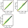 |
Fig. A.1. Relation between the true luminosity (x-axis) and RF predicted luminosity (y-axis) for the particles (20% of the total sample of ∼5 ⋅ 105) adopted for testing the performances of the trained RF algorithm. Results for the three predicted luminosities, i.e., [CII]158μm, [OI]63μm and [OI]145μm, are shown respectively in the left, middle and right panel. |
Appendix B: ALMA maps of [OI] 145μm, [CII], and continuum
This section summarizes the analysis of the new ALMA data considered in this work (Sect. 3). Visibilities were calibrated using the standard calibration provided by the ALMA observatory and the default phase, bandpass and flux calibrators. To model and subtract the continuum emission from the line, we combined the adjacent spectral windows in the baseband containing [OI] or [CII] and performed a fit in the uv plane to channels with |v|> 700 km s−1, using a first-order polynomial continuum. A continuum-subtracted datacube was created using CASA task tclean, with the hogbom cleaning algorithm in non-interactive mode, a threshold equal to two times the rms sensitivity and a natural weighting of the visibilities. We adopted a 30 km s−1 channel width. The resulting synthesized beam and rms sensitivity for a 30 km s−1 channel are listed in Table B.1. We created 0th moment maps by integrating over the emission line channels. Velocity-integrated line intensities were measured from 2D Gaussian fit of the 0th moment maps (Table B.1).
We created a continuum-subtracted ACA datacube of the [CII] emission in J204314−214439 following the approach described above, with an improved angular resolution (7.3×5.2 arcsec2) with respect to previous LMT observations (Zavala et al. 2015) following the same approach as described above. The resulting [CII] Oth moment map is shown in Fig. B.1 left. We detect three images with a similar [CII] line profile, two of which correspond to the double [OI] images detected in the ALMA map (Figure 1c). The velocity-integrated [CII] flux has been obtained by summing the three images is S[CII] = 25.62 ± 1.07 Jy km s−1.
A high resolution map (0.75×0.65 arcsec2) of the ∼362.7 GHz continuum in J204314−214439 was created by averaging the ALMA visibilities over all spectral windows (∼3 GHz) and excluding the channels of the [OI] emission, as shown in Figure B.1 right. By summing the fluxes of the three continuum sources in which we also detect [CII] 158μm and [OI] 145μm emission, we measure S3.7 = 24.47 ± 1.17 mJy.
New [OI] 145μm observations considered in this work.
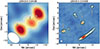 |
Fig. B.1. Left panel: [CII] emission map in J204314−214439. Contours correspond to [2, 3, 4, 5, 6, 8, 10, 15, 20, 30] σ confidence levels, where σ = 0.58 Jy beam−1 km s−1. The bottom-left white ellipse shows the ACA beam. Right panel: Continuum map at 362.7 GHz. Contours are as in left panel with σ = 0.12 mJy beam−1. Arrows indicate continuum sources in which we detect [OI] and [CII] emission. The bottom-left white ellipse shows the ALMA beam. |
Appendix C: Redshift evolution of scaling relations
Fig. C.1 shows the evolution of the SFR–luminosity relations for our simulated galaxies at redshifts z = 6, 8, and 10. We find that the [OI] 63μm and [OI] 145μm luminosities exhibit little to no redshift evolution, while the normalization of the SFR–[CII] relation increases slightly toward lower redshift. This trend is due to two competing effects: as redshift decreases, galaxies become more metal-enriched – particularly in carbon and oxygen – boosting line emission. Conversely, higher-redshift galaxies with similar SFRs tend to have higher gas densities. For [CII], metallicity enrichment dominates, leading to a modest redshift evolution in its luminosity. In contrast, the [OI] lines, which have higher critical densities, are more sensitive to gas density; thus, the two effects roughly balance, resulting in nearly redshift-invariant [OI] luminosities.
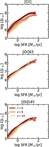 |
Fig. C.1. Relation between SFR and [CII] 158μm, [OI] 63μm and [OI] 145μm luminosity for our simulated galaxies at z = 6, 8, and 10. Solid lines refer to median trends, while shaded regions are 16th to 84th percentile dispersion. |
Consequently, also the line ratios [OI] 63μm/[CII] 158μm and [OI] 145μm/[CII] 158μm exhibit a redshift dependence, increasing by a factor of two to three at z = 8 − 10 relative to the z = 6 values discussed in Sect. 4.4.
Appendix D: [CII] luminosity
In this Appendix we show our model’s prediction for the [CII]-SFR relation in z ∼ 6 galaxies. Given the larger abundance of [CII] data at this redshift with respect to [OI], we use this line as a sort of check of our line emission modeling. Also, we need to check the reliability of the [CII] predictions since we discuss some line ratios with this line. The results are reported in Fig. D.1, where our theoretical predictions are compared with z ∼ 6 observations from the compilation of Ramos Padilla et al. (2023) and the objects with [OI] 63μm and/or [OI] 145μm detections adoped for comparison in this work (Sect. 3). The agreement up to the SFRs available in our simulation is good. In the high SFR end of our predictions there is a flattening of [CII] luminosity, due to the increasing abundance of CO and colder particles, which is at the origin of the well known [CII]/FIR deficit (e.g., Narayanan & Krumholz 2017). Such a prediction slightly deviates our model from the observations. However, we remark that a larger volume is needed to prove this high SFR regime.
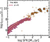 |
Fig. D.1. Relation between [CII] 158μm luminosity and SFR. Our simuation results at z = 6 are shown as red contours (solid line indicating the median trend). Observational data at z ≃ 6 compiled by Ramos Padilla et al. (2023) are shown as hexagons. We also include the high−z sources with [OI] 63μm and/or [OI] 145μm detections shown in the main text: REBELS galaxies (pentagons), A1689-zD1 (hexagon), J2054-0005 (star), J2310+1855 (cross), W2246-0526 (plus), J204314−214439 (diamond) and SPT0346−52 (small diamond). |
All Tables
Best-fitting parameters of the mass-to-light ratio as a function of physical quantities.
All Figures
|
Fig. 1. [OI] 145μm emission maps. Contour lines correspond to [2, 3, 4, 5, 6, 8, 10, 15, 20, 30] σ confidence levels, where σ = 0.030, 0.098, 0.082 and 0.024 Jy beam−1 km s−1 for panels a, b, c, and d, respectively. In panel c, arrows indicate the location in which we detect [OI] or [CII] emission at z = 4.680, in addition to continuum emission (Figure B.1). In each panel, the bottom-left white ellipse shows the ALMA beam. |
| In the text | |
|
Fig. 2. Visualization of the [OI] 63μm and [OI] 145μm luminosities, and the [OI] 63μm/[CII] 158μm and [OI] 145μm/[CII] 158μm ratios, for the most massive simulated galaxy at z = 6.14. Black contours follow the gas density distribution. |
| In the text | |
|
Fig. 3. Fraction of self-absorbed 63 μm [OI] line flux due to foreground material as a function of the galaxy SFR as predicted by our model. Solid lines refer to median trends while the shaded area are the 16th to 84th percentile dispersion. The solid line refers to the fiducial model, while the dashed one is obtained without considering the condition on velocity in Eq. (4). The yellow dashed region represent the typical values adopted in observational studies (reduction by a factor of two to four). |
| In the text | |
|
Fig. 4. Luminosity function of [OI] 63μm (top panel) and [OI] 145μm (bottom panel) at z = 6, 8, and 10 as predicted by our simulation. Errorbars are obtained by bootstrapping. The colored arrows in the top panel indicate the mean magnitude of the foreground self-absorption at each redshift. Low opacity points are those affected by resolution effects. |
| In the text | |
|
Fig. 5. Relations between the [OI] 63μm (red) and [OI] 145μm (blue) line luminosities and stellar mass (left), gas-phase metallicity traced by oxygen-to-hydrogen number ratio with respect to solar (middle), and H2 mass (right) for our simulated galaxies at z = 6. Solid lines represent the median trends, while density contours illustrate the underlying distribution of galaxies. |
| In the text | |
|
Fig. 6. Relation between [OI] 63μm (left panel) and [OI] 145μm (right panel) line luminosity and SFR. Our simulation results at z = 6 are shown as red density contours, with solid lines representing median trends. The median trend of the model with self-absorption neglecting the Eq. (4) condition is shown as a dashed line. Dotted lines are linear fits of the simulation results, with coefficients listed in Section 4.3. Other z ∼ 6 predictions for [OI] 63μm luminosity obtained from the post-processing of numerical simulations are also reported: Olsen et al. (2017) as blue circles and Ramos Padilla et al. (2023) as a turquoise area. Some observations are also reported for reference. The data up to z = 4 compiled by Ramos Padilla et al. (2023) are shown as hexagons. The J2054-00005 at z = 6.04 (Ishii et al. 2025) and W2246-0526 at z = 4.60 (Fernández Aranda et al. 2024) have both [OI] 63μm and [OI] 145μm detections. As for [OI] 145μm, we include the recent 6.5 ≤ z ≤ 7.7 REBELS observations (Fudamoto et al. 2025), the z = 6.00 J2310+1855 QSO (Li et al. 2020), and the new data obtained in this work (A1689-zD1 at z = 7.13, SPT0346−52 at z = 5.7 and J204313.2-214439 at z = 4.68; see Sect. 3). |
| In the text | |
|
Fig. 7. Line ratios as a function of SFR: [OI] 63μm/[CII] 158μm (top), [OI] 145μm/[CII] 158μm (middle) and [OI] 145μm/[OI] 63μm (bottom). Our simulation results at z = 6 are shown with red contours, with the solid line representing median trend. The median trend of the model with self-absorption neglecting the Eq. (4) condition is shown as a dashed line. The black arrows indicate the magnitude of the [OI] 63μm self-absorption by foreground gas as predicted by our model. Simulation predictions by Ramos Padilla et al. (2023) at z ∼ 6 are shown as turquoise contours. The same observational data shown in Fig. 6 are included where detections are available, as described in the legend. |
| In the text | |
|
Fig. 8. Distribution of the [OI] 145μm/[OI] 63μm and [OI] 63μm/[CII] 158μm line ratios for different values of [OI] 145μm/[CII] 158μm, as shown in the colorbar. The colored region represents the outcome of the PDR DESPOTIC computations assuming homogeneous clouds with 102 ≤ nH/cm−3 ≤ 106 and 20 ≤ T/K ≤ 104. Our simulated z ≃ 6 galaxies are shown as circles, J2054-0005 as a star, W2246-0526 as a plus and the SPT0346−52 upper limit as a diamond. The black arrow illustrates the typical shift due to [OI] 63μm foreground self-absorption. |
| In the text | |
|
Fig. 9. Mass-to-light ratio MH2/L[OI] for [OI] 63μm and [OI] 145μm, respectively in red and blue color scales. We report simulation predictions at z = 6 (contours) and linear fits for log(SFR/M⊙yr−1) ≥ −0.5. Observational results (Sect. 3) for REBELS galaxies (pentagons), A1689-zD1 (hexagon), J204313.2-214439 (diamond), SPT0346−52 (small diamond), W2246-0526 (plus), J2054-0005 (star), and J2310+1855 (cross) are also reported. |
| In the text | |
|
Fig. 10. [OI] 145μm luminosity and [OI] 145μm/[CII] 158μm ratio as a function of SFR for our model galaxies at z = 6. Different colors refer to different model assumptions in the post-processing pipeline with DESPOTIC. The red one represents the fiducial model adopted in this work, the cyan is a model where the CRs rate is scaled with the SFR density, the yellow and purple are models where the density profile is assumed to be logotropic and power-law. Solid lines refer to median trends and shaded regions indicate the 16th to 84th percentile dispersion. For reference, the available z ≳ 5 observations discussed in this work are also reported, with the same symbols as in Figs. 6 and 7. |
| In the text | |
|
Fig. A.1. Relation between the true luminosity (x-axis) and RF predicted luminosity (y-axis) for the particles (20% of the total sample of ∼5 ⋅ 105) adopted for testing the performances of the trained RF algorithm. Results for the three predicted luminosities, i.e., [CII]158μm, [OI]63μm and [OI]145μm, are shown respectively in the left, middle and right panel. |
| In the text | |
|
Fig. B.1. Left panel: [CII] emission map in J204314−214439. Contours correspond to [2, 3, 4, 5, 6, 8, 10, 15, 20, 30] σ confidence levels, where σ = 0.58 Jy beam−1 km s−1. The bottom-left white ellipse shows the ACA beam. Right panel: Continuum map at 362.7 GHz. Contours are as in left panel with σ = 0.12 mJy beam−1. Arrows indicate continuum sources in which we detect [OI] and [CII] emission. The bottom-left white ellipse shows the ALMA beam. |
| In the text | |
|
Fig. C.1. Relation between SFR and [CII] 158μm, [OI] 63μm and [OI] 145μm luminosity for our simulated galaxies at z = 6, 8, and 10. Solid lines refer to median trends, while shaded regions are 16th to 84th percentile dispersion. |
| In the text | |
|
Fig. D.1. Relation between [CII] 158μm luminosity and SFR. Our simuation results at z = 6 are shown as red contours (solid line indicating the median trend). Observational data at z ≃ 6 compiled by Ramos Padilla et al. (2023) are shown as hexagons. We also include the high−z sources with [OI] 63μm and/or [OI] 145μm detections shown in the main text: REBELS galaxies (pentagons), A1689-zD1 (hexagon), J2054-0005 (star), J2310+1855 (cross), W2246-0526 (plus), J204314−214439 (diamond) and SPT0346−52 (small diamond). |
| In the text | |
Current usage metrics show cumulative count of Article Views (full-text article views including HTML views, PDF and ePub downloads, according to the available data) and Abstracts Views on Vision4Press platform.
Data correspond to usage on the plateform after 2015. The current usage metrics is available 48-96 hours after online publication and is updated daily on week days.
Initial download of the metrics may take a while.