| Issue |
A&A
Volume 705, January 2026
|
|
|---|---|---|
| Article Number | A181 | |
| Number of page(s) | 10 | |
| Section | Extragalactic astronomy | |
| DOI | https://doi.org/10.1051/0004-6361/202557237 | |
| Published online | 19 January 2026 | |
Catching the 2021 γ-ray flare in the blazar TXS 2013+370
1
Department of Physics, Aristotle University of Thessaloniki 54124 Thessaloniki, Greece
2
Interdisziplinäres Zentrum für Wissenschaftliches Rechnen (IWR), Universität Heidelberg Im Neuenheimer Feld 205 69120 Heidelberg, Germany
3
Max-Planck-Institut für Radioastronomie Auf dem Hügel 69 D-53121 Bonn, Germany
4
INAF – Istituto di Radioastronomia Via P. Gobetti 101 40129 Bologna, Italy
5
Owens Valley Radio Observatory, California Institute of Technology Pasadena CA 91125, USA
6
Center for Astrophysics | Harvard & Smithsonian 60 Garden Street Cambridge MA 02138, USA
7
CSIRO, Space and Astronomy PO Box 76 Epping NSW 1710, Australia
8
Institut für Theoretische Physik und Astrophysik, Universität Würzburg Emil-Fischer-Str. 31 97074 Würzburg, Germany
9
Instituto Nacional de Astrofísica, Óptica y Electrónica Luis Enrique Erro #1 Tonantzintla Puebla 72840, Mexico
★ Corresponding author: This email address is being protected from spambots. You need JavaScript enabled to view it.
Received:
13
September
2025
Accepted:
18
November
2025
Abstract
The γ-ray–loud blazar TXS 2013+370, a powerful multiwavelength emitter at z = 0.859, underwent an exceptional gigaelectron volt outburst in late 2020 to early 2021. In this work, we present full polarization VLBI imaging at 22, 43, and 86 GHz (11 February 2021) together with contemporaneous single-dish monitoring (OVRO 15 GHz; SMA 226 GHz) and Fermi–LAT light curves to localize the high-energy dissipation site and probe the magnetic field of the inner jet. The images enabled us to study the jet structure and field topology on sub-parsec scales, revealing a compact near-core knot at r ≃ 40 − 60 μas along with the gigaelectron volt (GeV) flare and a flat core-dominated spectrum (α ≳ −0.5). The core has strong linear polarization and exhibits a ∼50° electric vector polarization angle rotation at 86 GHz. The pixel-based and integrated fits we employed yielded a high, uniform rotation measure, RM = (7.8 ± 0.2)×104 rad m−2, consistent with an external Faraday screen. Performing a cross-correlation of Fermi–LAT and 15 GHz light curves revealed a highly significant peak, with the γ rays leading by Δt = (102 ± 12) d. Adopting βapp = 4.2 ± 0.5 and θ = 4.1° ±0.2° implies a de-projected separation of Δrγ − 15 = (2.71 ± 0.47) pc and locates the GeV emission between the jet apex and ∼0.42 pc (in the 1σ range) downstream. Our results do not pinpoint the emission site; rather, they support two valid scenarios. The γ-ray production occurs within the broad-line region (∼0.07 pc), where external-Compton scatters optical/UV photons to γ-rays, and beyond the broad-line region, reaching ∼0.42 pc (1σ) within the inner parsecs, where external-Compton scattering of dusty-torus infrared photons dominates. Both scenarios are compatible in the allowed range of emission distances, while opacity-driven core shifts modulate the observed radio–γ delay without requiring large relocations of the dissipation zone.
Key words: galaxies: active / galaxies: jets / galaxies: magnetic fields / galaxies: nuclei / quasars: general / quasars: supermassive black holes
© The Authors 2026
 Open Access article, published by EDP Sciences, under the terms of the Creative Commons Attribution License (https://creativecommons.org/licenses/by/4.0), which permits unrestricted use, distribution, and reproduction in any medium, provided the original work is properly cited.
This article is published in open access under the Subscribe to Open model. This email address is being protected from spambots. You need JavaScript enabled to view it. to support open access publication.
1. Introduction
Blazars are the most extreme manifestation of active galactic nuclei. These objects feature relativistic plasma jets launched from supermassive black holes that are oriented close to our line of sight, and they emit violently across the electromagnetic spectrum (e.g., Urry & Padovani 1995; Ulrich et al. 1997; Sikora 2001; Cavaliere & D’Elia 2002). A key question that concerns the physical processes driving the γ-ray emission in jets is the location of its production site. Observational findings and theoretical models suggest that high-energy emission can originate in regions close to the central engine and further downstream in the jet (e.g., Jorstad et al. 2001; Rani et al. 2014; Patiño-Álvarez et al. 2019; Chavushyan et al. 2020, and references therein). To understand the physical mechanisms behind these emission processes, leptonic models provide a comprehensive theoretical framework. In this framework, the photons that are up-scattered by the relativistic leptons to γ-ray energies are either the same synchrotron photons radiated by the jet, i.e., synchrotron-self-Compton (Maraschi et al. 1992), or photons from the jet surroundings, i.e., external Compton (EC; e.g., Sikora et al. 1994; Ghisellini & Tavecchio 2008; Dermer et al. 2009). With increasing distance from the black hole, possible reservoirs of these seed photons include the accretion disk (Dermer et al. 1992), the broad-line region (BLR; e.g., Dermer & Schlickeiser 1993; Dotson et al. 2012), the dusty torus (Błażejowski et al. 2000; Kataoka et al. 1999), and even cosmic microwave background photons (Celotti & Ghisellini 2008).
Millimeter very long baseline interferometry (mm-VLBI) observations are particularly suited for investigating the γ-ray emission origin in blazars, especially when they are combined with broadband variability monitoring (e.g., Boccardi et al. 2017; Paraschos et al. 2023). While γ-ray detectors have a poor angular resolution (∼0.1° for Fermi-LAT at 1 GeV; Atwood et al. 2009), mm-VLBI provides extremely high resolution views of the innermost jet regions, which are unaffected by synchrotron opacity. Moreover, polarimetric VLBI observations probe the magnetic field configuration in relativistic jets, which is also crucial for particle acceleration (Paraschos et al. 2024a,b). Magnetohydrodynamic simulations have shown that as jets propagate, plasma instabilities develop toroidal components that aid in collimation and stability (McKinney & Blandford 2009; Lyutikov 2012) and thus directly influence particle acceleration through reconnection and shock processes (Sironi & Spitkovsky 2014; Sironi et al. 2015).
The compact radio source TXS 2013+370 is a powerful γ-ray loud blazar located at redshift z = 0.859 (Shaw et al. 2013), and it hosts a supermassive black hole with a mass of  M⊙ (Ghisellini & Tavecchio 2015), where the uncertainty reflects the 0.5–0.6 dex systematic error inherent to virial mass estimates (Vestergaard & Peterson 2006). Previous studies (Mukherjee et al. 2000; Halpern et al. 2001; Kara et al. 2012) established the firm association between TXS 2013+370 and a Fermi-Large Area Telescope (LAT) source through correlated radio and γ-ray variability, revealing a two-component spectral energy distribution best described by EC processes involving seed photons from a dusty torus environment. Subsequent VLBI studies by Traianou et al. (2020) constrained the γ-ray emission location to approximately 1 pc from the jet apex and revealed a transition from parabolic to conical jet expansion at parsec scales.
In this study, we investigate the morphological evolution, magnetic field structure, and spectral properties of the radio jet during an exceptional γ-ray flaring episode that began in December 2020. We conducted full polarimetric target of opportunity (ToO) observations using the Very Long Baseline Array (VLBA) plus Effelsberg at 22 and 43 GHz, and we complemented these with VLBA observations at 86 GHz, achieving angular resolutions down to ∼0.14 mas (∼1.1 pc). By combining VLBI imaging with kinematic analysis and correlated flux density variability across radio, millimeter-wave, and γ-ray bands, we constrained the γ-ray production region, probed the magnetic field topology, and investigated the spectral evolution in the innermost jet regions during this exceptional flare.
For our calculations, we adopted the following cosmological parameters: ΩM = 0.27, ΩΛ = 0.73, and H0 = 71 km s−1 Mpc−1 (similar to those used by Lister et al. 2016, and references therein), which result in a luminosity distance of DL = 5.489 Gpc and a linear-to-angular size conversion of 7.7 pc/mas for the redshift of z = 0.859.
2. Observations and data reduction
2.1. Data acquisition
The VLBI observations of TXS 2013+370 were performed on 11 February 2021 following elevated γ-ray emission from the source since 6 December 2020. Our VLBI datasets include polarimetric observations at 22 and 43 GHz with the full VLBA array plus Effelsberg and at 86 GHz with seven VLBA antennas. The data were recorded for 8 hours in two polarizations (left and right circular polarized, LCP and RCP) with a 64 MHz bandwidth per polarization split into four intermediate frequency (IF) bands of 16 MHz each. The observations followed a standard VLBI calibration strategy, alternating between the target source, TXS 2013+370, and the gain calibrators, 3C 345 and BL Lacertae. The details of the aforementioned VLBI observations are summarized in Table 1.
VLBI observational and polarimetric parameters of TXS 2013+370 on 11 February 2021.
2.2. Calibration
The data reduction was performed using the National Radio Astronomy Observatory’s Astronomical Image Processing System (AIPS; Greisen 1990). AIPS is a widely used software package for VLBI calibration, and it was used in the present work for all three frequencies: 22 GHz, 43 GHz, and 86 GHz. The calibration procedure starts with the correction of phase errors in the cross-correlation data introduced by the sampler and is followed by a parallactic angle correction of the phases. After the initial corrections, we performed manual phase calibration to determine the delay, phase errors, and rate corrections using fringe-fitting per baseline and high signal-to-noise ratio scans. After achieving phase alignment across the observing band and time for each baseline, global fringe fitting was performed to solve for the residual delays and phase errors with respect to the reference antenna. With the phases calibrated, we proceeded to visibility amplitude calibration. After updating the Tsys and gain tables in AIPS, we performed absolute flux calibration, converting the observed visibility data into flux density values. We then applied amplitude calibration, incorporating corrections for atmospheric opacity, which were derived using the measured system temperatures and the gain-elevation curves of each telescope. The polarization alignment was performed using the RLDLY task on a bright scan of the source. The removal of instrumental polarization leakage from the data, also known as D-terms (Leppänen et al. 1994), was performed via the task LPCAL in AIPS following the process described in detail, along with the absolute electric vector polarization angle (EVPA) calibration, in Appendix A.1.
2.3. Imaging and model fitting
The total intensity and polarization images of TXS 2013+370 at 22 GHz, 43 GHz, and 86 GHz were produced using Difmap (Shepherd 1997). The amplitude and phase calibrated data were imported into Difmap, where spurious data points were flagged and removed following careful inspection of the visibility amplitudes and phases. Images were created using the CLEAN deconvolution algorithm, an iterative procedure implemented in Difmap, producing three radio maps at the respective frequencies (see Fig. 1). For all three maps, the jet brightness distribution was parameterized using the MODELFIT algorithm in Difmap. This procedure fits two-dimensional Gaussian components to the fully calibrated visibility data, providing a quantitative description of the flux density distribution along the jet direction. Component uncertainties were formally computed based on the local signal-to-noise ratio (S/N) in the image surrounding each component (Fomalont 1999; Lobanov 2005; Schinzel et al. 2012). However, for the flux density uncertainty, we adhered to more conservative criteria by following the methodology described in Traianou et al. (2024, 2025), and references therein, as the formal errors obtained via this method appeared too small. All parameters of the fit Gaussian components are provided in Table 2. Given that TXS 2013+370 lies very close to the Galactic plane, interstellar scattering effects could potentially affect the radio images due to the high column density of the interstellar medium along the line of sight. However, as demonstrated by Traianou et al. (2020) through detailed analysis of interstellar scattering effects on VLBI data, such effects are dominant only at longer centimeter wavelengths for TXS 2013+370, with a threshold frequency of approximately 10 GHz. Therefore, our millimeter-wavelength observations are essentially unaffected by interstellar scattering, ensuring reliable morphological analysis of the innermost jet regions.
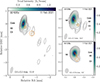 |
Fig. 1. Total intensity images of TXS 2013+370 from 11 February 2021. Left: Observations at 22 GHz. Top-right: Observations at 43 GHz. Bottom-right: Observations at 86 GHz. Contours are at 0.5, 1, 2, 4, 8, 16, 32, and 64% of each panel’s peak (22: 1.33 Jy/beam; 43: 0.75 Jy/beam; 86: 0.71 Jy/beam). Restoring beams are shown as gray ellipses (parameters in Table 1). Orange circles mark MODELFIT Gaussian centroids. The 43 GHz map resolves a new knot (N2) near the core. At 86 GHz, the compact core and components (A2, C3, and N2) are clearly detected. |
2.4. Single-dish radio light curves and Fermi-LAT data
Single-dish observations were provided by the 40-m telescope of the Owens Valley Radio Observatory (OVRO) at 15 GHz and the eight-element Submillimeter Array (SMA)1 at 226 GHz. The γ-ray data were obtained by Fermi-LAT and are from the fourth LAT source catalog (Abdollahi et al. 2023), with 1-month binning in the 0.1–100 GeV energy range. All measurements span approximately the same period, from 2008 to 2025. As shown in the multi-frequency light curves presented in Fig. 2, the source exhibited significant activity during our monitoring period, with two major flaring episodes occurring in 2021 and 2024. Our VLBI observations were conducted during the 2021 flare, which is clearly visible across all frequency bands.
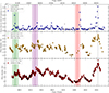 |
Fig. 2. Light curves of the blazar TXS 2013+370 at different frequencies. From top to bottom: Fermi-LAT 0.1–100 GeV with 1-month binning, flux plotted vs. time for 226 GHz SMA, and 15 GHz OVRO. The dashed vertical lines indicate the estimated ejection times of the components N, N1 (Traianou et al. 2020), and the new knot N2, respectively, whereas the width of the shadow areas designates the uncertainty of these estimations. For N2, the uncertainty is based on the uncertainty of component A1 as it was found in Traianou et al. (2020). The dashed gray line indicates a new flaring activity in the source. |
3. Data analysis and results
3.1. Source structure and jet components
Our multi-frequency VLBI observations at 22, 43, and 86 GHz reveal TXS 2013+370 as a compact, core-dominated source with a curved jet structure extending southwestward from the bright core region. The total intensity images (Fig. 1) show a well-defined morphology consisting of a dominant core and several distinct jet components, with the overall jet structure becoming increasingly well-resolved at higher frequencies. In addition to the N2, we identified stationary features A2 and C3, whose positions and flux densities are consistent with the quasi-stationary components reported by Traianou et al. (2020). At 22 GHz, the source displays a relatively simple structure with a bright, unresolved core and extended emission along the jet direction. The core dominates the total flux density with 1.32 Jy (92% of the total flux), while the jet components contribute the remaining emission. The 43 GHz observations reveal additional structural details. Most significantly, these observations enable the detection of component N2, a newly emerged feature located approximately 60 μas from the VLBI core. This component exhibits a flux density of 330 ± 30 mJy at 43 GHz and is likely associated with the enhanced multiwavelength activity observed during our monitoring period. Such associations between newly emerged VLBI components and γ-ray flares are common in blazars, with ∼83% of GeV outbursts coinciding with new superluminal features in the VLBA-BU-BLAZAR monitoring program (Jorstad et al. 2017). At the highest frequency (86 GHz), component N2 is clearly visible with a flux density of 550 ± 60 mJy, while the core becomes more compact at this frequency, with a density of 210 ± 20 mJy.
The Gaussian model-fitting analysis (presented in Table 2) helped us quantify the jet curved morphology which has position angles ranging from approximately –126° for component N2 to –160° for the more distant component, C3. Component sizes increase systematically with distance from the core (20–400 μas), consistent with adiabatic jet expansion. The flux density distribution among the components varies significantly with frequency, reflecting the different opacity conditions across the jet. At 86 GHz, where synchrotron opacity effects are minimal, component N2 contributes a significant fraction of the total emission after the core, taking the leading role in the flaring episode.
Model-fitting parameters for TXS 2013+370.
3.2. Spectral decomposition
We reconstructed the spectral index along the jet using quasi-simultaneous image pairs at 22–43 and 43–86 GHz, adopting the definition Sν ∝ ν+α. For each frequency pair, all maps were convolved by a common restoring beam corresponding to the equivalent circular beam of the higher frequency, following standard practice (e.g., Traianou et al. 2024), and a pixel size of 18 μas. Image alignment was performed via 2D cross-correlation (Gabuzda et al. 2004) in which the lower-frequency map was held fixed, while the higher-frequency map was systematically shifted pixel-by-pixel to maximize the cross-correlation coefficient between the two intensity distributions. This approach is appropriate when optically thin jet features suitable for direct component-based alignment are not available or when core shifts are below the resolution limit. For TXS 2013+370, Traianou et al. (2020) have demonstrated that core shifts between 15 and 86 GHz are ≲0.1 mas, well below our beam sizes, justifying a correlation-based alignment method. The resulting shifts are (Δx, Δy) = (0, +1) pixels at 22–43 GHz and ( − 2, +1) pixels at 43–86 GHz. Through visual inspection, we confirmed the physically consistent spectral structures in the aligned maps. The resulting maps are shown in Fig. 3.
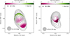 |
Fig. 3. Spectral index distributions of TXS 2013+370. The contour levels are set to 0.5, 1, 2, 4, 8, 16, 32, and 64% Jy/beam of the peak flux density of the highest frequency map in the pair (see Table 1) and represent the total intensity contours. All the images are convolved with a common beam that was set equal to the equivalent circular beam b = (bmaxbmin)1/2 of the highest frequency, and each frequency pair was aligned using a 2D cross-correlation analysis. Left: Frequency pair of 22-43 GHz. Right: Frequency pair of 43–86 GHz. |
The spectral index maps show relatively uniform, flat spectra in the core region across all frequency pairs, with some steeper indices appearing in the outer jet regions where signal-to-noise ratios are lower. To quantify the core spectral properties, we computed a representative value by applying a mask (64% of the peak of the highest frequency map in the pair) to calculate the average of the indices within the first contour, with uncertainties following Bartolini et al. (2025). From the results, we noticed that the VLBI core exhibits spectral indices of αcore = −0.43 ± 0.01 at 22–43 GHz and −0.51 ± 0.11 at 43–86 GHz, with a mean value α ≳ −0.5, indicating a flat spectrum characteristic of partially self-absorbed emission. The consistency of these values across both frequency pairs suggests stable spectral properties during the flare epoch.
3.3. Polarization and Faraday rotation
The polarimetric VLBI data of the source at 22 GHz and, for the first time, at 43 and 86 GHz (calibration in Appendix A.1) reveal a core with strong, coherent linear polarization and a well-aligned magnetic field (Fig. 4). The fractional linear polarization reaches 3.3 ± 0.5% (22 GHz), 4.5 ± 0.6% (43 GHz), and 3.5 ± 0.8% (86 GHz), with EVPAs of 109 ± 4°, 113.0 ± 0.5°, and 52 ± 8°, respectively (Table 1). The EVPA uncertainties follow Hovatta et al. (2012), calculated by combining in quadrature the single-dish reference angle error (∼3.6° for 22 GHz, ∼0.5° for 43 GHz, and ∼7.9° for 86 GHz) and the propagated error, with the latter derived from the rms of the Q/U maps and a 10% calibration term.
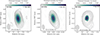 |
Fig. 4. Polarization images of TXS 2013+370 observed on 11 February 2021. Left: Polarized-intensity map at 22 GHz with EVPA vectors (white sticks) overplotted. Middle: Polarization image at 43 GHz. Right: Polarization image at 86 GHz. Contours are at 0.5, 1, 2, 4, 8, 16, 32, and 64% of each panel’s peak (22 GHz: 1.31 Jy /beam; 43 GHz: 0.80 Jy /beam; 86 GHz: 0.70 Jy /beam), and they represent the total intensity contours. The restoring beam is shown as a gray ellipse in the lower-left corner. |
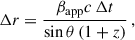
A notable feature in our images is a sudden ∼50° EVPA rotation at 86 GHz, which changes the inferred magnetic field orientation from roughly parallel to nearly perpendicular to the jet axis. This behavior may indicate a change in field geometry (e.g., helical with toroidal-to-poloidal dominance; Gabuzda et al. 2004; O’Neill et al. 2019), though opacity effects cannot be excluded. To test this, we corrected for Faraday rotation by calculating the rotation measure (RM) for each pixel (e.g., Algaba 2013) using
 (1)
(1)
where χ(λ) is the observed EVPA, χ0 is the intrinsic EVPA, and λ is the observing wavelength. We derived the pixel-based RM by linearly fitting χ versus λ2 for each pixel, explicitly unwrapping nπ ambiguities following Hovatta et al. (2012). Only pixels with polarized intensities exceeding 3σP were used, and a relaxed χ2 threshold ensured robust fits across the core. In addition, an integrated RM value for the core was obtained by fitting the frequency-averaged U and Q, yielding a result consistent with the pixel-based analysis.
The RM map presented in Fig. 5 reveals a high and uniform RM = (7.81 ± 0.16)×104 rad m−2, with uncertainties from the covariance matrix of the per-pixel fits lying within a narrow range across the core region. These values significantly exceed typical blazar-core RMs of 102–104 rad m−2 (e.g., Hovatta et al. 2012; Algaba 2013). The RM distribution shows high uniformity with no strong transverse gradients and is accompanied by a ∼50° EVPA rotation between 22–43 GHz and 86 GHz. The physical interpretation of these findings is discussed in Sect. 4.4.
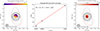 |
Fig. 5. Faraday rotation results for the blazar TXS 2013+370. Left: Pixel-based map of intrinsic RM. Dashed lines correspond to the outermost total intensity contours of the 22 GHz (black) and 43 GHz (red) maps. Solid contours are set to 2, 4, 8, 16, 32, and 64% of the 86 GHz peak polarized intensity (0.70 Jy /beam). All maps have been convolved with a common beam, the equivalent circular beam of the 86 GHz map, which is shown as a gray circle in the bottom-left corner. Middle: Linear fit of Eq. (1) after unwrapping the nπ ambiguities showing EVPA rotation from 86 GHz to 22 GHz. The slope yields an integrated RM of (7.81 ± 0.16)×104 rad m−2 for the core region. Right: Pixel-based map of RM uncertainties from the covariance matrix of the per-pixel least-square fits. |
3.4. Multiband variability
To investigate the connection between γ-ray and radio variability, we performed a comprehensive correlation analysis. We first established the reality of γ-radio associations across the complete 16-year observational record (2008-2025; Fig. 2). We defined γ-ray flares as periods where the Fermi-LAT flux exceeds 3 × 10⁻⁷ photons per square centimetre per second (approximately three times the quiescent level) for more than 30 days, identifying five prominent events. Radio flares were defined as enhancements in the OVRO 15 GHz light curve exceeding 3.0 Jy (approximately 1.3 times the baseline level of ∼2.3 Jy) sustained for more than 15 days, yielding ten distinct radio flares. We used OVRO data for this analysis, as the SMA 226 GHz observations exhibit significantly higher variability noise and sparser observational cadence, which obscures clear flare identification.
To assess statistical significance, we performed Monte Carlo simulations by randomly shuffling the five γ-ray flare occurrence times (keeping ten radio flare times fixed) across the 16-year observation window. For each of the 10 000 trials, we counted how many γ-ray flares had an associated radio flare within ±200-day windows. Only 130 trials showed four or more associations (matching our observed 4/5 success rate), yielding p = 0.013. This demonstrates that the observed γ-radio correlation is unlikely to arise from random temporal overlap. The γ-ray flares were defined as periods with flux greater than 3 × 10⁻⁷ photons per square centimetre per second, sustained for more than 30 days and the radio flares as flux greater than 3.0 Jy sustained for more than 15 days. These thresholds were chosen to capture major outbursts clearly visible in Fig. 2 while avoiding identification of variability noise as flares.
We then applied quantitative cross-correlation analysis using the discrete cross-correlation function (DCCF; Edelson & Krolik 1988) between the Fermi-LAT and OVRO 15 GHz light curves on a 6 d lag grid (requiring eight or more pairs per bin) for the 2019–2022 interval. This setup provided homogeneous sampling and a single, coherent activity state. The amplitude significance was assessed using a power spectral density plus a probability density function to generate matched surrogate γ-ray light curves following Emmanoulopoulos et al. (2013). We generated 5000 realizations, cross-correlated each with the 15 GHz data, and derived the 95% and 99% confidence envelopes as a function of lag.
The γ-15 GHz DCCF shows a prominent peak of r = 0.67 ± 0.09 at a lag of 102 days, corresponding to a 7.7σ significance, well above the 99% confidence envelope (derived from 1000 autoregressive AR(1) surrogate pairs), confirming a highly significant correlation. The time lag and its uncertainty were obtained via flux randomization and random subset selection Monte Carlo resampling (e.g., Peterson et al. 1998). For each set of 5000 realizations, we perturbed the fluxes by their errors and bootstrap-resampled the time series, recomputed the DCCF, and measured a weighted centroid of the peak using points with r ≥ 0.9 rmax within a region of interest centered on the observed peak (half-width set by the DCCF FWHM, ≃65 d, with a minimum of 60 d). We adopted the median lag and the 16th–84th percentiles as the 1σ statistical interval and added in quadrature a small resolution floor that reflects the data binning and cadence. This yields a γ-ray lead of Δt = (102 ± 12) days (Fig. 6).
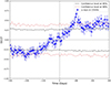 |
Fig. 6. Results of the DCCF between the γ-ray and 15 GHz light curves. Positive time lags indicate that γ-ray activity leads the activity in radio. The significance of the correlations is displayed by a dashed line for the 2σ level and by a dotted line for the 3σ level. |
4. Discussion
4.1. Location of the γ-ray emission
A strong correlation was found between the γ-ray and 15 GHz variability, indicating that the high-energy activity leads the radio by Δt = (102 ± 12) days. Following Pushkarev et al. (2010), this observed time lag can be translated into the de-projected linear distance, Δr, between the γ-ray and 15 GHz emission zones with
 (2)
(2)
where βapp is the plasma apparent speed (in units of c) and θ is the jet viewing angle. Because our single-epoch dataset does not allow for direct determination of βapp and θ, we adopted the values from Traianou et al. (2020) for the innermost moving component A1, βapp = 4.2 ± 0.5, and θ = 4.1° ±0.2°. We emphasize that this speed represents the inner jet (< 0.5 mas from the core). While 15 GHz VLBI monitoring shows higher speeds (βapp ∼ 14) at larger distances, Traianou et al. (2020) have demonstrated clear velocity stratification, with Γ ∼ 6 in the inner jet increasing to Γ > 14 at parsec scales, reflecting ongoing jet acceleration. Using outer-jet speeds would overestimate the γ-ray location (Δr ∼ 8 pc), placing the emission site at distances (∼6 pc) inconsistent with particle energization in the acceleration zone. With these parameters and the measured lag, we obtained Δrγ − 15 = (2.71 ± 0.47) pc, where the uncertainty was calculated by propagating errors in quadrature from the lag measurement (12 d) and the uncertainties on βapp and θ. Considering the reported jet geometry and the presence of a recollimation shock just downstream of the VLBI core (Traianou et al. 2020), we adopted R ≤ (2.05 ± 0.97) pc as the de-projected distance of the 15 GHz core from the jet apex. The location of the γ-ray emission is then rγ ≡ R − Δr = 2.05 − 2.71 = −0.66 ± 1.08 pc. This formally negative value, while carrying large uncertainties that span from upstream of the apex to ∼0.42 pc downstream, indicates that the γ-ray site likely lies between the jet apex and the 15 GHz core, consistent with the observed γ-ray lead in the light curves. This is compatible with the rγ ∼ 0.75 ± 1.26 pc (or ∼1 pc) location found by Traianou et al. (2020) for the 2009 flare. On these scales, and given the FSRQ nature of TXS 2013+370, the relevant external seed photons for inverse Compton scattering are those of the BLR and the dusty torus. Therefore, we interpret these constraints as an indication that the γ-ray emission region likely lies within the BLR or exceeds it, entering the torus environment and reaching distances of ∼0.42 pc in the 1σ range.
Our conclusions do not lead to the exact location of the emission site. Instead, they permit two plausible interpretations: (1) With a BLR size of ∼0.07 pc (Traianou et al. 2020), the emission region is fully compatible with locations closer to the base of the jet, where optical and UV BLR-photons get up-scattered to high-energies via EC. (2) Our inferred γ-ray site lies beyond or at the BLR edge, making the dusty torus the primary photon reservoir, with infrared photons intercepted by the jet and up-scattered to γ-rays also via EC. It is also highly possible that both the BLR and the dusty torus actively contribute to shaping the high-energy output of TXS 2013+370. Nonetheless, in Traianou et al. (2020), they constrained the location of the γ-ray emission on scales of 1–2 parsecs from the central engine, concluding that the dusty torus is the best candidate for providing a rich seed photon field. Additionally, in Kara et al. (2012), they showed that the SED modeling of TXS 2013+370 required the existence of an external radiation field with low temperatures (T ∼ 102 K) in order to find the best possible fit for the dominant emitting region, indicating an origin from cold dust. Taking into account the previous studies, it seems that the scale tips toward one scenario and thus favors the dusty torus as the most possible seed photon reservoir. Our results are positioned in the intersection of these analyses, yielding strong insights that, indeed, the dusty torus is a possible seed photon field, but the BLR cannot be neglected, as it is an equally likely possibility.
4.2. Temporal comparison of γ-ray emission sites and knots
Our two well-studied flares (in 2009 and late 2021) place the γ-ray dissipation region in the same inner-parsec neighborhood despite differing γ–15 GHz lags. For the 2009 flare (Traianou et al. 2020), the lag analysis locates the γ-ray zone at ∼1 pc downstream of the jet apex – beyond the BLR and naturally compatible with EC on dusty-torus photons (e.g., Błażejowski et al. 2000; Ghisellini & Tavecchio 2008; Dermer et al. 2009). For the 2021 outburst, our DCCF yields a robust γ–15 GHz lead of (102 ± 12) d, implying a separation of (2.71 ± 0.47) pc between the γ site and the 15 GHz core. Combined with the upper limit to the 15 GHz core–apex distance (R15 ≲ 2.05 ± 0.97 pc), this bounds the γ-ray location to ∼0–0.42 pc (1σ) downstream of the apex. Thus, both epochs point to sub-parsec and parsec scales, in the torus-dominated EC regime, though this study also supports the BLR domain as an equal possibility.
The differing lags we see between the two events are most naturally attributed to changes in the inner-jet state rather than relocations of the dissipation site. In 2021, we detected a compact near-core knot, a flat core-dominated spectrum, and coherent millimeter polarization signatures of enhanced particle and magnetic energy densities around the core. These conditions increase synchrotron opacity and shift the 15 GHz core downstream, lengthening the γ–15 GHz delay even if rγ is unchanged (e.g., Schinzel et al. 2012). By contrast, the shorter 2009 lag is consistent with a less opaque core and/or a flare that couples more directly to a downstream standing feature within the same spatial zone (e.g., Karamanavis et al. 2016; Rani et al. 2016). For context, simple peak-to-peak offsets during the 2024 activity (MJDγ = 60398, MJD1 mm = 60418, MJD15 GHz = 60421) give Δtγ − 1 mm = 20 d and Δtγ − 15 GHz = 23 d, indicative separations of ≃0.53 pc and ≃0.61 pc for the same geometry. Although sensitive to cadence and flare asymmetry, the frequency ordering and scales reinforce a stable inner-parsec γ-ray site and a recollimation-shock nature of the VLBI core.
Parsec-scale γ-ray zones similar to our result are widely reported. For instance, in the BL Lacs AO 0235+164 and OJ 287, major flares arise ≳12–14 pc downstream, co-spatial with the millimeter core and the standing features (Agudo et al. 2011b,a). Among FSRQs, 3C 454.3 links GeV outbursts to superluminal knots crossing the 43 GHz core (Jorstad et al. 2013), PKS 1222+216 shows very high-energy emission beyond the BLR (Tavecchio et al. 2011), and PKS 1510−089 often favors parsec-scale sites near the millimeter core, with episodes from multiple zones (Orienti et al. 2013; Brown 2013; H.E.S.S. Collaboration & MAGIC Collaboration 2021). Even for 3C 273, rapid flares constrain the GeV region to ≲1.6 pc (Rani et al. 2013). Collectively, these studies place many strong γ-ray outbursts ∼0.1 pc to a few parsecs from the apex, consistent with our findings for TXS 2013+370. Finally, decade-long multiwavelength/polarimetric monitoring of CTA 102 indicates zero-lag correlations between γ-ray and optical emission over multiple cycles, implying co-spatiality between the optical emission zone and the seed photon reservoir for γ-ray production on timescales of years (Ma et al. 2025).
4.3. Core spectral properties and particle acceleration
The flat core spectral indices (α ≳ −0.5) measured across both 22–43 and 43–86 GHz frequency pairs indicate partially self-absorbed synchrotron emission in the VLBI core region during the 2021 flare. Such flat spectra are characteristic of inhomogeneous jets, and they can be shaped by a standing recollimation shock near the core or by the superposition of traveling shocks downstream (e.g., Marscher 1977; Marscher et al. 2008). The temporal association between the flat spectrum and the emergence of component N2 suggests ongoing particle injection and efficient acceleration during the flare. The measured spectral indices are consistent with shock-accelerated electron distributions with a power-law index of p ≃ 2 − 2.2, corresponding to optically thin spectral indices of αthin ≃ −0.5 to −0.6 (Bell 1978; Blandford & Ostriker 1978). While these values favor shock acceleration as the primary particle energization mechanism (Marscher et al. 2008), contributions from magnetic reconnection cannot be excluded (Mimica et al. 2009; Sironi & Spitkovsky 2014), particularly given the complex magnetic field structure revealed by our polarimetric observations (Sect. 3.3). We note that in-beam blending effects, particularly at 22 GHz, where the synthesized beam is larger, may affect the measured core spectral index. Extended jet emission within the beam could contribute additional flux to the core component, potentially flattening the observed spectrum. If the true core flux is lower than measured, the intrinsic spectral index could be even flatter (α ∼ 0), further supporting a scenario of sustained particle injection in a partially self-absorbed core region. Nevertheless, the consistency between the 22–43 and 43–86 GHz pairs, which probe different spatial scales, suggests that beam blending is not the dominant effect shaping the observed flat spectrum.
4.4. Faraday rotation: External screen versus intrinsic jet effects
The exceptionally high RM = (7.81 ± 0.16)×104 rad m−2, significantly exceeds typical blazar-core values and requires interpretation. Two scenarios can explain this situation: an external Faraday screen or intrinsic jet opacity effects. The spatial uniformity of the RM and lack of transverse gradients favor an external screen, likely associated with the Galactic interstellar medium. TXS 2013+370 lies close to the Galactic plane (b ∼ 2°) in the Cygnus region, where high column densities of magnetized plasma are well-documented (Traianou et al. 2020). The ∼50° EVPA rotation between 43 and 86 GHz is naturally explained by wavelength-dependent Faraday rotation (χ ∝ λ2). Internal jet processes would typically produce spatial RM gradients, which are not observed. However, opacity effects cannot be excluded. The EVPA flip at 86 GHz could reflect increasing transparency in the jet base, which would reveal intrinsic EVPA variations from jet curvature and helical magnetic field geometry (Gabuzda et al. 2004; O’Neill et al. 2019) rather than true Faraday rotation. In this scenario, frequency-dependent opacity would cause the observed λ2 EVPA behavior without actual RM. While both scenarios remain viable, the RM uniformity and the established Galactic foreground along this sight line (Traianou et al. 2020) favor the external screen interpretation. Nonetheless, multi-epoch polarimetric observations are needed to distinguish between these scenarios. In general, external screens tend to produce stable RM values, while opacity effects should vary with jet activity.
5. Summary and conclusions
In this work, we conducted polarimetric VLBI observations of TXS 2013+370 at 22, 43, and 86 GHz during an exceptional GeV outburst on 11 February 2021, achieving angular resolutions down to ∼0.1 mas. This represents the first multi-frequency polarimetric VLBI study of this source. Our main findings are as follows:
-
We successfully detected a new jet component, moving outward from the VLBI core, during enhanced activity. Our imaging revealed a curved jet with a newly emerged component, N2, located ∼60 μas from the core associated with enhanced multiwavelength activity. Spectral analysis showed flat indices (α ≳ −0.5), indicating ongoing particle acceleration.
-
TXS 2013+370 experiences strong linear polarization and exceptionally high Faraday rotation. Polarimetric observations revealed strong coherent polarization (3.3–4.5%) and an exceptionally high Faraday RM of (7.81 ± 0.16)×104 rad m−2, indicating propagation through a dense, magnetized external screen. However, as these are the first Faraday results for TXS 2013+370, internal jet opacity effects cannot be excluded as a possible origin of the EVPA swing.
-
We localized the γ-ray emission site to a range of distances from the jet origin. Cross-correlation analysis revealed a highly significant γ-ray lead of (102 ± 12) days over 15 GHz emission, corresponding to a separation of (2.71 ± 0.47) pc. Combined with the core-apex distance constraint from Traianou et al. (2020), we locate the γ-ray emission at ( − 0.66 ± 1.08) pc but with a large uncertainty that spans from the jet apex to ∼0.42 pc. This is consistent with sub-parsec scales favoring both the BLR and the dusty torus environments.
-
The γ-ray production region remains stable despite the variable delays. While the 2009 and 2021 flares show different γ-ray to radio delays, both locate the γ-ray emission within sub-parsec to parsec scales, indicating that lag variations reflect changing opacity conditions rather than a moving dissipation site.
-
The inferred location of the γ-ray flare supports external Compton scattering models. Our results demonstrate that γ-ray production occurs in a spatially stable region in TXS 2013+370 and is anchored to specific jet features, challenging simple one-zone models and supporting scenarios where EC scattering on BLR and/or dusty torus photons dominate the high-energy emission.
This work provides constraints on the high-energy emission site of TXS 2013+370 and delivers the first detailed view of its magnetic field geometry at 43 and 86 GHz. Our analysis offers new insights into γ-ray production in blazars and into the magnetic field topologies that shape relativistic jets, contributing to the broader effort to understand their high-energy output and the physical conditions of their innermost regions. We also shed light on the origin of Faraday rotation in this source, identifying the presence of a possible external Faraday screen. However, future multi-epoch VLBI observations at millimetre wavelengths will be crucial for determining whether the observed EVPA rotation arises from an external Galactic screen or from opacity-driven internal processes. Time-resolved polarimetric monitoring could track the evolution of the magnetic field geometry and test for the presence of helical fields in the innermost jet. Additionally, extending the spectral analysis to higher frequencies and combining these observations with simultaneous γ-ray monitoring during future flaring episodes would provide tighter constraints on particle acceleration mechanisms and the location of high-energy emission sites. Such observations are already available from GMVA monitoring at 43 and 86 GHz conducted over a two-year interval, offering a promising avenue for follow-up studies.
Acknowledgments
I would like to especially thank Prof. P. Papadopoulos for his invaluable contributions, mentoring, and support throughout this work. His lectures and discussions made the analysis and the paper writing an inspiring and rewarding journey of discovery. We also thank the anonymous referee for the valuable comments and suggestions, which greatly improved the paper. This research has made use of data from the OVRO 40-m monitoring program (Richards et al. 2011), which is supported in part by NASA grants NNX08AW31G, NNX11A043G, and NNX14AQ89G and NSF grants AST-0808050 and AST-1109911. The Submillimeter Array is a joint project between the Smithsonian Astrophysical Observatory and the Academia Sinica Institute of Astronomy and Astrophysics and is funded by the Smithsonian Institution and the Academia Sinica. This research has made use of NASA’s Astrophysics Data System. The Fermi-LAT Collaboration acknowledges the generous ongoing support from a number of agencies and institutes that have supported both the development and the operation of the LAT, as well as scientific data analysis. These include the National Aeronautics and Space Administration and the Department of Energy in the United States; the Commissariat á l’Energie Atomique and the Centre National de la Recherche Scientifique/Institut National de Physique Nucléaire et de Physique des Particules in France; the Agenzia Spaziale Italiana and the Istituto Nazionale di Fisica Nucleare in Italy; the Ministry of Education, Culture, Sports, Science and Technology (MEXT), High Energy Accelerator Research Organization (KEK), and Japan Aerospace Exploration Agency (JAXA) in Japan; and the K. A. Wallenberg Foundation, the Swedish Research Council, and the Swedish National Space Board in Sweden. Additional support for science analysis during the operations phase is gratefully acknowledged from the Istituto Nazionale di Astrofisica in Italy and the Centre National d’Etudes Spatiales in France. This work was performed in part under DOE Contract DE-AC02-76SF00515. We recognize that Maunakea is a culturally important site for the indigenous Hawaiian people; we are privileged to study the cosmos from its summit. This work was supported by the Max Planck Institute for Radioastronomy (MPIfR) - Mexico Max Planck Partner Group led by V.M.P.-A. This publication includes data based on observations with the 100-m telescope of the MPIfR at Effelsberg.
References
- Abdollahi, S., Ajello, M., Baldini, L., et al. 2023, ApJS, 265, 31 [NASA ADS] [CrossRef] [Google Scholar]
- Agudo, I., Jorstad, S. G., Marscher, A. P., et al. 2011a, ApJ, 726, L13 [NASA ADS] [CrossRef] [Google Scholar]
- Agudo, I., Marscher, A. P., Jorstad, S. G., et al. 2011b, ApJ, 735, L10 [NASA ADS] [CrossRef] [Google Scholar]
- Agudo, I., Thum, C., Molina, S. N., et al. 2017, MNRAS, 474, 1427 [Google Scholar]
- Algaba, J. C. 2013, MNRAS, 429, 3551 [Google Scholar]
- Atwood, W. B., Abdo, A. A., Ackermann, M., et al. 2009, ApJ, 697, 1071 [CrossRef] [Google Scholar]
- Bartolini, V., Dallacasa, D., Gómez, J. L., et al. 2025, A&A, 698, A123 [NASA ADS] [CrossRef] [EDP Sciences] [Google Scholar]
- Bell, A. R. 1978, MNRAS, 182, 147 [Google Scholar]
- Blandford, R. D., & Ostriker, J. P. 1978, ApJ, 221, L29 [Google Scholar]
- Błażejowski, M., Sikora, M., Moderski, R., & Madejski, G. M. 2000, ApJ, 545, 107 [Google Scholar]
- Boccardi, B., Krichbaum, T. P., Ros, E., & Zensus, J. A. 2017, A&ARv, 25, 4 [NASA ADS] [CrossRef] [Google Scholar]
- Brown, A. M. 2013, MNRS, 431, 824 [Google Scholar]
- Cavaliere, A., & D’Elia, V. 2002, ApJ, 571, 226 [NASA ADS] [CrossRef] [Google Scholar]
- Celotti, A., & Ghisellini, G. 2008, MNRAS, 385, 283 [NASA ADS] [CrossRef] [Google Scholar]
- Chavushyan, V., Patiño-Álvarez, V. M., Amaya-Almazán, R. A., & Carrasco, L. 2020, ApJ, 891, 68 [CrossRef] [Google Scholar]
- Dermer, C. D., & Schlickeiser, R. 1993, ApJ, 416, 458 [Google Scholar]
- Dermer, C. D., Schlickeiser, R., & Mastichiadis, A. 1992, A&A, 256, L27 [NASA ADS] [Google Scholar]
- Dermer, C. D., Finke, J. D., Krug, H., & Böttcher, M. 2009, ApJ, 692, 32 [NASA ADS] [CrossRef] [Google Scholar]
- Dotson, A., Georganopoulos, M., Kazanas, D., & Perlman, E. S. 2012, ApJ, 758, L15 [Google Scholar]
- Edelson, R. A., & Krolik, J. H. 1988, ApJ, 333, 646 [Google Scholar]
- Emmanoulopoulos, D., McHardy, I. M., & Papadakis, I. E. 2013, MNRAS, 433, 907 [NASA ADS] [CrossRef] [Google Scholar]
- Fomalont, E. B. 1999, ASP Conf. Ser., 180, 301 [NASA ADS] [Google Scholar]
- Gabuzda, D. C., Pushkarev, A. B., & Cawthorne, T. V. 2004, MNRAS, 350, 529 [Google Scholar]
- Ghisellini, G., & Tavecchio, F. 2008, MNRAS, 386, L28 [NASA ADS] [CrossRef] [Google Scholar]
- Ghisellini, G., & Tavecchio, F. 2015, MNRAS, 448, 1060 [NASA ADS] [CrossRef] [Google Scholar]
- Gómez, J. L., Traianou, E., Krichbaum, T. P., et al. 2022, ApJ, 924, 122 [Google Scholar]
- Greisen, E. W. 1990, in Acquisition, Processing and Archiving of Astronomical Images, eds. G. Longo, & G. Sedmak, 125 [Google Scholar]
- H.E.S.S. Collaboration& MAGIC Collaboration. 2021, A&A, 648, A23 [NASA ADS] [CrossRef] [EDP Sciences] [Google Scholar]
- Halpern, J. P., Eracleous, M., Mukherjee, R., & Gotthelf, E. V. 2001, ApJ, 551, 1016 [Google Scholar]
- Hovatta, T., Lister, M. L., Aller, M. F., et al. 2012, AJ, 144, 105 [Google Scholar]
- Jorstad, S. G., Marscher, A. P., Mattox, J. R., et al. 2001, ApJ, 556, 738 [NASA ADS] [CrossRef] [Google Scholar]
- Jorstad, S. G., Marscher, A. P., Smith, P. S., et al. 2013, ApJ, 773, 147 [Google Scholar]
- Jorstad, S. G., Marscher, A. P., Morozova, D. A., et al. 2017, ApJ, 846, 98 [Google Scholar]
- Kara, E., Errando, M., Max-Moerbeck, W., et al. 2012, ApJ, 746, 159 [Google Scholar]
- Karamanavis, V., Fuhrmann, L., Krichbaum, T. P., et al. 2016, A&A, 586, A60 [NASA ADS] [CrossRef] [EDP Sciences] [Google Scholar]
- Kataoka, J., Mattox, J. R., Quinn, J., et al. 1999, ApJ, 514, 138 [NASA ADS] [CrossRef] [Google Scholar]
- Leppänen, K. J., Zensus, J. A., & Diamond, P. D. 1994, in Compact Extragalactic Radio Sources, eds. J. A. Zensus, & K. I. Kellermann, 207 [Google Scholar]
- Lister, M. L., Aller, M. F., Aller, H. D., et al. 2016, AJ, 152, 12 [NASA ADS] [CrossRef] [Google Scholar]
- Lobanov, A. P. 2005, arXiv e-prints [arXiv:astro-ph/0503225] [Google Scholar]
- Lyutikov, M. 2012, MNRAS, 419, 3048 [Google Scholar]
- Ma, C.-L., Deng, J.-H., & Jiang, Y.-G. 2025, ApJ, 990, 82 [Google Scholar]
- Maraschi, L., Ghisellini, G., & Celotti, A. 1992, ApJ, 397, L5 [CrossRef] [Google Scholar]
- Marscher, A. P. 1977, AJ, 82, 781 [Google Scholar]
- Marscher, A. P., Jorstad, S. G., D’Arcangelo, F. D., et al. 2008, Nature, 452, 966 [Google Scholar]
- McKinney, J. C., & Blandford, R. D. 2009, MNRAS, 394, L126 [Google Scholar]
- Mimica, P., Aloy, M.-A., Agudo, I., et al. 2009, ApJ, 696, 1142 [NASA ADS] [CrossRef] [Google Scholar]
- Mukherjee, R., Gotthelf, E. V., Halpern, J., & Tavani, M. 2000, ApJ, 542, 740 [Google Scholar]
- O’Neill, S., Kiehlmann, S., Readhead, A. C. S., et al. 2019, MNRAS, 490, 1961 [CrossRef] [Google Scholar]
- Orienti, M., Koyama, S., D’Ammando, F., et al. 2013, MNRAS, 428, 2418 [Google Scholar]
- Paraschos, G. F., Mpisketzis, V., Kim, J. Y., et al. 2023, A&A, 669, A32 [NASA ADS] [CrossRef] [EDP Sciences] [Google Scholar]
- Paraschos, G. F., Debbrecht, L. C., Kramer, J. A., et al. 2024a, A&A, 686, L5 [NASA ADS] [CrossRef] [EDP Sciences] [Google Scholar]
- Paraschos, G. F., Wielgus, M., Benke, P., et al. 2024b, A&A, 687, L6 [NASA ADS] [CrossRef] [EDP Sciences] [Google Scholar]
- Patiño-Álvarez, V. M., Dzib, S. A., Lobanov, A., & Chavushyan, V. 2019, A&A, 630, A56 [NASA ADS] [CrossRef] [EDP Sciences] [Google Scholar]
- Peterson, B. M., Wanders, I., Horne, K., et al. 1998, PASP, 110, 660 [Google Scholar]
- Pushkarev, A. B., Kovalev, Y. Y., & Lister, M. L. 2010, ApJ, 722, L7 [NASA ADS] [CrossRef] [Google Scholar]
- Rani, B., Krichbaum, T. P., Marscher, A. P., et al. 2013, A&A, 557, A71 [NASA ADS] [CrossRef] [EDP Sciences] [Google Scholar]
- Rani, B., Krichbaum, T. P., Marscher, A. P., et al. 2014, A&A, 571, L2 [NASA ADS] [CrossRef] [EDP Sciences] [Google Scholar]
- Rani, B., Krichbaum, T. P., Hodgson, J. A., & Zensus, J. A. 2016, JPCS, 718, 052032 [Google Scholar]
- Richards, J. L., Max-Moerbeck, W., Pavlidou, V., et al. 2011, ApJS, 194, 29 [Google Scholar]
- Schinzel, F. K., Lobanov, A. P., Taylor, G. B., et al. 2012, A&A, 537, A70 [NASA ADS] [CrossRef] [EDP Sciences] [Google Scholar]
- Shaw, M. S., Romani, R. W., Cotter, G., et al. 2013, ApJ, 764, 135 [NASA ADS] [CrossRef] [Google Scholar]
- Shepherd, M. C. 1997, ASP Conf. Ser., 125, 77 [Google Scholar]
- Sikora, M. 2001, AIP Conf. Proc., 558, 275 [Google Scholar]
- Sikora, M., Begelman, M. C., & Rees, M. J. 1994, ApJ, 421, 153 [Google Scholar]
- Sironi, L., & Spitkovsky, A. 2014, ApJ, 783, L21 [NASA ADS] [CrossRef] [Google Scholar]
- Sironi, L., Petropoulou, M., & Giannios, D. 2015, MNRAS, 450, 183 [Google Scholar]
- Tavecchio, F., Becerra-Gonzalez, J., Ghisellini, G., et al. 2011, A&A, 534, A86 [CrossRef] [EDP Sciences] [Google Scholar]
- Traianou, E., Krichbaum, T. P., Boccardi, B., et al. 2020, A&A, 634, A112 [NASA ADS] [CrossRef] [EDP Sciences] [Google Scholar]
- Traianou, E., Krichbaum, T. P., Gómez, J. L., et al. 2024, A&A, 682, A154 [NASA ADS] [CrossRef] [EDP Sciences] [Google Scholar]
- Traianou, E., Gómez, J. L., Cho, I., et al. 2025, A&A, 700, A16 [NASA ADS] [CrossRef] [EDP Sciences] [Google Scholar]
- Ulrich, M.-H., Maraschi, L., & Urry, C. M. 1997, ARA&A, 35, 445 [NASA ADS] [CrossRef] [Google Scholar]
- Urry, C. M., & Padovani, P. 1995, PASP, 107, 803 [NASA ADS] [CrossRef] [Google Scholar]
- Vestergaard, M., & Peterson, B. M. 2006, ApJ, 641, 689 [Google Scholar]
Appendix A: Calibration of the instrumental polarization
A.1. Polarization leakage and D-terms
The polarization calibration was performed in AIPS using the LPCAL task, which estimates the D-terms for each intermediate frequency (IF) independently. We used TXS 2013+370 itself as the polarization calibrator, providing LPCAL with a Stokes I source model derived from our imaging process. LPCAL employs a linear fitting algorithm that requires polarization leakage < 5% and good parallactic angle coverage for accurate results. The VLBA antennas achieved large parallactic angle coverage (≥100°, reaching ∼200°), resulting in leakages < 5%. However, Effelsberg showed limited coverage (∼15°), leading to ∼15% leakage at 22 GHz and unreliable values at 43 GHz. Comparison of calibration results with and without Effelsberg showed that this antenna provided no additional information for the new jet component, only confirming the core EVPA already determined by VLBA data. Therefore, we excluded Effelsberg from polarization analysis while retaining its data for total intensity imaging.
The computed D-terms for VLBA antennas showed consistent values across all IFs, with dispersions of ∼2.4% in amplitude and ∼77.7° in phase for 22 GHz, ∼1.7% and ∼94.2° for 43 GHz, and ∼6.9% and ∼93.2° for 86 GHz. For each antenna, we calculated median values across the IFs as representative D-terms.
Absolute EVPA calibration was performed using quasi-simultaneous single-dish observations from the POLAMI monitoring program.2 For 22 and 43 GHz, we used polarization angles measured on 9 February 2021 (109° ±3.6° at 13 mm) and 10 February 2021 (113.9° ±0.5° at 7 mm), respectively. For 86 GHz, we used Cubic Spline interpolation between the polarization angle and time, from historical POLAMI data, to obtain via extrapolation 51.9° ±7.9° for 11 February 2021.
We also estimated the polarization parameters and their uncertainties for all datasets, following Gómez et al. (2022), with the results presented in Table 1. The parameters were computed using data above a threshold of 5 × rms, where rms is an estimation of the map thermal noise.
 |
Fig. A.1. D-terms for the VLBA observations at 22, 43, and 86 GHz for RCP and LCP. Plotted values correspond to the medians of four IFs, with errors computed from the standard deviation across all IFs. |
All Tables
VLBI observational and polarimetric parameters of TXS 2013+370 on 11 February 2021.
All Figures
|
Fig. 1. Total intensity images of TXS 2013+370 from 11 February 2021. Left: Observations at 22 GHz. Top-right: Observations at 43 GHz. Bottom-right: Observations at 86 GHz. Contours are at 0.5, 1, 2, 4, 8, 16, 32, and 64% of each panel’s peak (22: 1.33 Jy/beam; 43: 0.75 Jy/beam; 86: 0.71 Jy/beam). Restoring beams are shown as gray ellipses (parameters in Table 1). Orange circles mark MODELFIT Gaussian centroids. The 43 GHz map resolves a new knot (N2) near the core. At 86 GHz, the compact core and components (A2, C3, and N2) are clearly detected. |
| In the text | |
|
Fig. 2. Light curves of the blazar TXS 2013+370 at different frequencies. From top to bottom: Fermi-LAT 0.1–100 GeV with 1-month binning, flux plotted vs. time for 226 GHz SMA, and 15 GHz OVRO. The dashed vertical lines indicate the estimated ejection times of the components N, N1 (Traianou et al. 2020), and the new knot N2, respectively, whereas the width of the shadow areas designates the uncertainty of these estimations. For N2, the uncertainty is based on the uncertainty of component A1 as it was found in Traianou et al. (2020). The dashed gray line indicates a new flaring activity in the source. |
| In the text | |
|
Fig. 3. Spectral index distributions of TXS 2013+370. The contour levels are set to 0.5, 1, 2, 4, 8, 16, 32, and 64% Jy/beam of the peak flux density of the highest frequency map in the pair (see Table 1) and represent the total intensity contours. All the images are convolved with a common beam that was set equal to the equivalent circular beam b = (bmaxbmin)1/2 of the highest frequency, and each frequency pair was aligned using a 2D cross-correlation analysis. Left: Frequency pair of 22-43 GHz. Right: Frequency pair of 43–86 GHz. |
| In the text | |
|
Fig. 4. Polarization images of TXS 2013+370 observed on 11 February 2021. Left: Polarized-intensity map at 22 GHz with EVPA vectors (white sticks) overplotted. Middle: Polarization image at 43 GHz. Right: Polarization image at 86 GHz. Contours are at 0.5, 1, 2, 4, 8, 16, 32, and 64% of each panel’s peak (22 GHz: 1.31 Jy /beam; 43 GHz: 0.80 Jy /beam; 86 GHz: 0.70 Jy /beam), and they represent the total intensity contours. The restoring beam is shown as a gray ellipse in the lower-left corner. |
| In the text | |
|
Fig. 5. Faraday rotation results for the blazar TXS 2013+370. Left: Pixel-based map of intrinsic RM. Dashed lines correspond to the outermost total intensity contours of the 22 GHz (black) and 43 GHz (red) maps. Solid contours are set to 2, 4, 8, 16, 32, and 64% of the 86 GHz peak polarized intensity (0.70 Jy /beam). All maps have been convolved with a common beam, the equivalent circular beam of the 86 GHz map, which is shown as a gray circle in the bottom-left corner. Middle: Linear fit of Eq. (1) after unwrapping the nπ ambiguities showing EVPA rotation from 86 GHz to 22 GHz. The slope yields an integrated RM of (7.81 ± 0.16)×104 rad m−2 for the core region. Right: Pixel-based map of RM uncertainties from the covariance matrix of the per-pixel least-square fits. |
| In the text | |
|
Fig. 6. Results of the DCCF between the γ-ray and 15 GHz light curves. Positive time lags indicate that γ-ray activity leads the activity in radio. The significance of the correlations is displayed by a dashed line for the 2σ level and by a dotted line for the 3σ level. |
| In the text | |
|
Fig. A.1. D-terms for the VLBA observations at 22, 43, and 86 GHz for RCP and LCP. Plotted values correspond to the medians of four IFs, with errors computed from the standard deviation across all IFs. |
| In the text | |
Current usage metrics show cumulative count of Article Views (full-text article views including HTML views, PDF and ePub downloads, according to the available data) and Abstracts Views on Vision4Press platform.
Data correspond to usage on the plateform after 2015. The current usage metrics is available 48-96 hours after online publication and is updated daily on week days.
Initial download of the metrics may take a while.