| Issue |
A&A
Volume 705, January 2026
|
|
|---|---|---|
| Article Number | A260 | |
| Number of page(s) | 22 | |
| Section | Planets, planetary systems, and small bodies | |
| DOI | https://doi.org/10.1051/0004-6361/202557304 | |
| Published online | 27 January 2026 | |
Sibling sub-Neptunes around sibling M dwarfs: TOI-521 and TOI-912
1
Instituto de Astrofísica de Canarias (IAC),
38205
La Laguna, Tenerife,
Spain
2
Departamento de Astrofísica, Universidad de La Laguna (ULL),
38206
La Laguna, Tenerife,
Spain
3
Instituto de Astrofísica de Andalucía (IAA-CSIC), Glorieta de la Astronomía s/n,
18008
Granada,
Spain
4
Department of Astronomy & Astrophysics, University of Chicago,
Chicago,
IL
60637,
USA
5
Department of Social Data Science, Hitotsubashi University,
2-1 Naka, Kunitachi,
Tokyo
186-8601,
Japan
6
Institut d’Estudis Espacials de Catalunya (IEEC), Edifici RDIT, Campus UPC,
08860
Castelldefels (Barcelona),
Spain
7
Institut de Ciències de l’Espai (ICE, CSIC), Campus UAB, c/ de Can Magrans s/n,
08193
Cerdanyola del Vallès, Barcelona,
Spain
8
Centro de Astrobiología (CSIC-INTA),
Crta. Ajalvir km 4,
28850
Torrejón de Ardoz, Madrid,
Spain
9
Univ. Grenoble Alpes, CNRS, IPAG,
38000
Grenoble,
France
10
Institute of Astronomy, Faculty of Physics, Astronomy and Informatics, Nicolaus Copernicus University,
Grudziądzka 5,
87-100
Toruń,
Poland
11
Komaba Institute for Science, The University of Tokyo,
3-8-1 Komaba, Meguro,
Tokyo
153-8902,
Japan
12
Astrobiology Center,
2-21-1 Osawa, Mitaka,
Tokyo
181-8588,
Japan
13
National Astronomical Observatory of Japan,
2-21-1 Osawa, Mitaka,
Tokyo
181-8588,
Japan
14
Department of Astronomical Science, The Graduate University for Advanced Studies (SOKENDAI),
2-21-1 Osawa, Mitaka,
Tokyo
181-8588,
Japan
15
Department of Physics and Astronomy, The University of Western Ontario,
1151 Richmond St,
London, Ontario,
N6A 3K7,
Canada
16
UTokyo Organization for Planetary and Space Science,The University of Tokyo,
7-3-1 Hongo, Bunkyo,
Tokyo
113-0033,
Japan
17
Kapteyn Astronomical Institute, University of Groningen,
PO Box 800,
9700
AV
Groningen,
The Netherlands
18
Graduate School of Environmental, Life, Natural Science and Technology, Okayama University,
3-1-1 Tsushima-naka, Kita,
Okayama
700-8530,
Japan
19
Center for Astrophysics | Harvard & Smithsonian,
60 Garden Street,
Cambridge,
MA
02138,
USA
20
NASA Ames Research Center,
Moffett Field,
CA
94035,
USA
21
Centre for Space and Habitability, Universität Bern,
Gesellschaftsstrasse 6,
3012
Bern,
Switzerland
22
ETH Zurich, Department of Physics,
Wolfgang-Pauli-Strasse 2,
8093
Zurich,
Switzerland
23
Departamento de Matemática y Física Aplicadas, Universidad Católica de la Santísima Concepción, Alonso de Rivera
2850,
Concepción,
Chile
24
Department of Physics & Astronomy, Texas Tech University,
Lubbock
TX,
79409-1051,
USA
25
Observatori Astronòmic Albanyà, Camí de Bassegoda S/N, Albanyà
17733,
Girona,
Spain
26
Department of Multi-Disciplinary Sciences, The University of Tokyo,
3-8-1 Komaba, Meguro,
Tokyo
153-8902,
Japan
27
Institute for Astronomy, University of Hawaii,
640 N. Aohoku Place,
Hilo,
HI
96720,
USA
28
SUPA Physics and Astronomy, University of St. Andrews, Fife,
KY16 9SS
Scotland,
UK
29
Okayama Observatory, Kyoto University,
3037-5 Honjo, Kamogata, Asakuchi,
Okayama
719-0232,
Japan
30
SETI Institute,
Mountain View,
CA
94043,
USA
31
Department of Physical Sciences, Ritsumeikan University,
1-1-1 Noji-higashi, Kusatsu,
Shiga
525-8577,
Japan
32
Trottier Space Institute at McGill, McGill University,
3550 University Street,
Montreal,
QC
H3A 2A7,
Canada
33
Subaru Telescope, National Astronomical Observatory of Japan,
650 N. Aohoku Place,
Hilo,
HI
96720,
USA
34
Institute of Engineering, Tokyo University of Agriculture and Technology,
2-24-26 Nakacho, Koganei,
Tokyo,
184-8588,
Japan
35
South African Astronomical Observatory,
PO Box 9, Observatory,
Cape Town
7935,
South Africa
36
Department of Physics and Kavli Institute for Astrophysics and Space Research, Massachusetts Institute of Technology,
Cambridge,
MA
02139,
USA
37
Kotizarovci Observatory,
Sarsoni 90,
51216
Viskovo,
Croatia
38
CAS Key Laboratory of Optical Astronomy, National Astronomical Observatories, Chinese Academy of Sciences,
Beijing
100101,
PR
China
★ Corresponding author: This email address is being protected from spambots. You need JavaScript enabled to view it.
Received:
18
September
2025
Accepted:
21
November
2025
Abstract
Context. Sub-Neptunes are absent in the Solar System, yet they are the most common category of planets found in our Galaxy. This kind of planet challenges the internal structure models, prompts investigations into its formation and evolution, and pushes atmospheric characterisation studies to break the degeneracy in their inner composition.
Aims. We report here the discovery and characterisation of new sub-Neptunes orbiting two similar M dwarfs, TOI-521 (Teff = 3544 ± 100 K, V = 14.7 mag) and TOI-912 (Teff = 3572 ± 100 K, V = 12.7 mag). Each star hosts a transiting planetary candidate identified by TESS and is part of the THIRSTEE follow-up programme, which aims to understand the sub-Neptune population through in-depth and precise characterisation studies on a population level.
Methods. We analysed TESS light curves, ground-based photometry, and high-precision ESPRESSO, HARPS, and IRD radial velocities to confirm the planetary nature of both candidates, infer the precise orbital and physical parameters of the planets, and investigate the presence of additional planets in the systems.
Results. The two stars host nearly identical planets in terms of mass and radius. TOI-521 hosts a transiting sub-Neptune in a 1.5-day orbit with radius and mass of Rb = 1.98 ± 0.14 R⊕ and Mb = 5.3 ± 1.0 M⊕, respectively. Moreover, we identified an additional candidate at 20.3 days, with a minimum mass of Mp sin i = 10.7−2.4+2.5 M⊕, currently not detected as transiting in our photometric dataset. Similarly, the planet orbiting TOI-912 is a 4.7-d sub-Neptune with Rb = 1.93 ± 0.13 R⊕ and Mb = 5.1 ± 0.5 M⊕. Interestingly, TOI-912 b likely possesses an unusually high eccentricity (e = 0.58 ± 0.02) and is probably undergoing strong tidal dissipation. If such eccentricity were confirmed, it would make TOI-912 b one of the most eccentric sub-Neptunes known to date. TOI-521 b and TOI-912 b have very similar densities (~4 g cm−3), and they lie in the degenerate region of the mass-radius diagram where different compositions are plausible, including a volatile-rich composition, or a rocky core surrounded by a H-He envelope. When compared to the other THIRSTEE M-dwarf targets, our sample supports the division of sub-Neptunes into two distinct populations divided by a density gap. Both planets are interesting targets for atmospheric follow-up in the context of understanding the temperature-atmospheric feature trend that starts to emerge thanks to JWST observations.
Key words: planets and satellites: composition / planets and satellites: detection / planets and satellites: individual: TOI-521 / planets and satellites: individual: TOI-912
NHFP Sagan Fellow.
© The Authors 2026
 Open Access article, published by EDP Sciences, under the terms of the Creative Commons Attribution License (https://creativecommons.org/licenses/by/4.0), which permits unrestricted use, distribution, and reproduction in any medium, provided the original work is properly cited.
This article is published in open access under the Subscribe to Open model. This email address is being protected from spambots. You need JavaScript enabled to view it. to support open access publication.
1 Introduction
The origin and nature of the sub-Neptune population is currently one of the big open questions in the exoplanetary community. These small planets (1 R⊕< Rp< 4 R⊕) are ubiquitous in the solar vicinity (e.g. Batalha et al. 2013; Petigura et al. 2013; Biazzo et al. 2022), yet no such planet exists in our Solar System. When considering their radius distribution, smaller planets, the so-called super-Earths (Rp≲ 1.4 R⊕), are commonly thought to have a rocky composition, while planets with bigger radii, especially in the 1.4 R⊕ ≲ Rp ≲ 2 R⊕ regime, could be explained assuming different internal compositions, and different formation and evolution processes (Rogers & Seager 2010). The two most common theories to explain the distribution and properties of these planets are: (1) based on atmospheric mass-loss processes (e.g. Owen & Wu 2013; Ginzburg et al. 2018; Gupta & Schlichting 2019; Rogers et al. 2023), according to which these planets are rocky cores surrounded by a variable amount of H/He atmospheres, or (2) based on volatile-rich theories (e.g. Bitsch et al. 2019; Izidoro et al. 2022; Burn et al. 2021) that claim that these planets formed outside the water ice line and are therefore rich in water, in quantities of up to 50% of their total mass. Currently, detailed models assuming more realistic and complex conditions for the planetary interiors are being developed, including atmosphere-magma ocean interactions (Schlichting & Young 2022; Misener et al. 2023; Rogers et al. 2024; Gupta et al. 2025), effects of high irradiation on atmospheres and water content (Turbet et al. 2020; Aguichine et al. 2021), and miscibility of water in the planetary interior (Dorn & Lichtenberg 2021; Luo et al. 2024). In this context, studying the atmospheric features of well-characterised planets is of primary importance, as it can provide additional observational constraints to unveil the composition and history of sub-Neptunes. The initial JWST studies of sub-Neptunes atmospheres have already shown promising results, highlighting the detection of atmospheric features and tentative trends within this population (Madhusudhan et al. 2023; Benneke et al. 2024; Piaulet-Ghorayeb et al. 2024; Davenport et al. 2025).
Within this active and growing field, the THIRSTEE project, described in Lacedelli et al. (2024), is currently trying to shed light on the nature and origin of sub-Neptunes through an observational approach, enlarging the sample of well-characterised sub-Neptunes orbiting both M-dwarf and FGK stars and studying their atmospheres, with the final aim of performing demographic analysis on such systems taking into account all their observed properties. Here, we present the discovery and characterisation of two new sub-Neptunes orbiting the M-dwarf stars TOI-521 and TOI-912, as part of the THIRSTEE sample.
2 TESS photometry
TESS observed TOI-521 and TOI-921 for a total of seven and six sectors, respectively (see summary of observations in Table A.1). The Science Processing Operations Center (SPOC) pipeline at NASA Ames Research Center (Jenkins et al. 2016; Jenkins 2020) reduced and analysed image data and identified a transiting candidate around each star; namely, TOI-521.01 (with period P ≃ 1.54 d) and TOI-912.01 (P ≃ 4.68 d).
For both stars we analysed the two-minute cadence Presearch Data Conditioning Simple Aperture Photometry (PDCSAP, Smith et al. 2012; Stumpe et al. 2012, 2014) light curves, reduced with the SPOC pipeline (see field of view of the targets and photometric aperture in Fig. A.1). For the photometric analysis, we selected from the PDCSAP only ‘good-quality’ data points (DQUALITY=01), and we clipped 3σ outliers, masking the in-transit points according to the ephemeris provided on the TESS Follow-up Observing Program (TFOP2; Collins 2019) to avoid affecting the transit shape.
3 Ground-based follow-up observations
We report here all the ground-based observations used in this work, including the ground-based transit observations collected as part of TFOP, long-term photometric monitoring, and high-precision spectroscopic observations. Observations are summarised in Table A.1, and all ground-based transit light-curves are shown in Fig. A.3. Appendix A also reports the high-resolution speckle imaging we carried out to provide confirmation for TOI-521.01 and TOI-912.01, which reveals no close companions to both stars within the angular and magnitude limits.
3.1 Transit photometry
ExTrA. We observed TOI-912.01 with the Exoplanets in Transits and their Atmospheres (ExTrA) facility (Bonfils et al. 2015) located at La Silla Observatory, Chile. We collected ten transits on separate nights, but various transits were simultaneously observed by more than one of the three 0.6-m telescopes in the facility, resulting in a total of 23 light curves. All observations were gathered with the 8-arcsec fibre, in the low-resolution mode of the spectrograph, and with an exposure time of 60 seconds. Data were reduced with the custom reduction software detailed in Cointepas et al. (2021).
LCOGT. We observed three full transit windows of TOI-521.01 from the Las Cumbres Observatory Global Telescope (LCOGT) (Brown et al. 2013) 1 m network nodes at McDonald Observatory near Fort Davis, Texas, United States (McD), Siding Spring Observatory near Coonabarabran, Australia (SSO), and Cerro Tololo Inter-American Observatory in Chile (CTIO). We also observed three full transits of TOI-912.01 from LCOGT 1 m network nodes at South Africa Astronomical Observatory near Sutherland, South Africa (SAAO), CTIO, and SAAO, respectively. The images were calibrated using the standard LCOGT BANZAI pipeline (McCully et al. 2018) and differential photometric data were extracted using AstroImageJ (Collins et al. 2017). We used circular photometric apertures with radii in the range of ![Mathematical equation: $\[5^{\prime \prime}_\cdot 0{-}7^{\prime \prime}_\cdot3\]$](/articles/aa/full_html/2026/01/aa57304-25/aa57304-25-eq2.png) , which excluded flux from all known Gaia DR3 catalogue neighbours that are bright enough to have hosted a blended nearby eclipsing binary that could have masqueraded as the TESS-detected transit.
, which excluded flux from all known Gaia DR3 catalogue neighbours that are bright enough to have hosted a blended nearby eclipsing binary that could have masqueraded as the TESS-detected transit.
MuSCAT2. We collected one full transit of TOI-521.01 with the multi-colour camera MuSCAT2 (Narita et al. 2019), mounted on the Telescopio Carlos Sànchez at the Teide Observatory. The exposure time of the four MuSCAT2 bands (g, r, i, and zs) was set to 15, 30, 30, and 45 s, respectively. Data were reduced and calibrated with the MuSCAT2 pipeline (Parviainen et al. 2019), which optimises the photometric aperture while performing the transit fit.
MEarth. We observed a full transit of TOI-912.01 with the MEarth South facility (Nutzman & Charbonneau 2008; Irwin et al. 2015) at the Cerro Tololo Inter-American Observatory, Chile. We extracted the photometry with a circular aperture of ![Mathematical equation: $\[7^{\prime \prime}_\cdot 1\]$](/articles/aa/full_html/2026/01/aa57304-25/aa57304-25-eq3.png) through a custom pipeline outlined in Irwin et al. (2007) and Berta et al. (2012).
through a custom pipeline outlined in Irwin et al. (2007) and Berta et al. (2012).
3.2 Long-term photometric monitoring
We used the All-Sky Automated Survey for Supernovae (ASAS-SN3 (Shappee et al. 2014; Kochanek et al. 2017) and Zwicky Transient Facility4 (ZTF, Bellm et al. 2019; Masci et al. 2019) long-term photometry to investigate stellar activity and search for the rotational period of the stars. TOI-912 ASAS-SN observations span between 2014-2018 (V filter) and 2018-2024 (g filter), for a total time span of ~1583 and ~2318 days, respectively. No ZTK observations are available for this star.
TOI-521 was observed by ASAS-SN between 2012-2018 (V filter) and 2017-2024 (g filter) for a total time span of ~2505 and ~2423 days, respectively. The star was also observed in the ZTF r filter between 2018 and 2024, for a total baseline of ~2216 d.
For all light curves, we selected only observations flagged as good-quality (QUALITY=G for ASAS-SN, and catflags=0 for ZTK), and we performed a 5σ clipping to remove outliers. Figs. C.1 and C.2 show the resulting light curves.
3.3 Spectroscopic observations
ESPRESSO. We followed-up both stars within the THIRSTEE programme with the ESPRESSO spectrograph (Pepe et al. 2021) on the ESO Very Large Telescope telescope array. We used ESPRESSO’s high-resolution mode (1 arcsec fibre, R ~ 140 000) with the 2 × 1 detector binning (HR21) on a single Unit Telescope (1UT), and we placed fibre B on the sky for background subtraction.
For TOI-521, we collected 22 data points (Program 112.25F2.001, PI: E. Palle) between November 13, 2023, and March 15, 2024, spanning a total of ~123 days. The adopted exposure time was 1800 seconds, implying a median signal-to-noise ratio (S/N) of 19 at 550 nm. We reduced the data with the ESPRESSO’s data reduction pipeline (DRS), and we extracted the radial velocities (RVs) using a M3 mask to compute the cross-correlation function (CCF). In our global analysis, we removed one spectrum that was collected in bad observing conditions, resulting in a low S/N ratio, and with an associated internal uncertainty of >3 m s−1 (3σ outlier).
For TOI-912, we collected 33 data points (Programs 111.24PJ. 001 and 113.26NP.001, PI: E. Palle), between April 10, 2023, and August 11, 2024, spanning a total of ~488 days. The exposure time was 900 seconds, implying a median S/N of 31 at 550 nm. Given the higher number of spectra, and the brightness of the target, which allows for a high S/N spectral template, in this case we extracted the RVs with the template-matching SERVAL5 algorithm (Zechmeister et al. 2018), which provided more precise median internal uncertainties and a smaller root mean square (RMS). The resulting RV datasets for the two stars (available on CDS) have an RMS of 5.3 m s−1 and 2.8 m s−1 and a median internal uncertainty of 1.5 m s−1 and 0.47 m s−1, respectively.
IRD. We collected 65 RVs for TOI-521 with the InfraRed Doppler (IRD) spectrograph at the Subaru 8.2-m telescope (Tamura et al. 2012; Kotani et al. 2018), under the Subaru/IRD intensive programmes S19A-069I, S20B-088I, S21B-118I, and S23A-067I (PI: N. Narita). The observing campaign spanned between April 18, 2019 and April 7, 2023, for a total observational baseline of ~1450 days. The integration time per exposure ranged from 180 to 1800 s, depending on the observing condition for each night, and the raw data were reduced following Kuzuhara et al. (2018); Hirano et al. (2020), while RVs were extracted in the manner outlined in Hirano et al. (2020) and Kuzuhara et al. (2024). We excluded from the dataset three points collected in bad observing conditions, resulting in a low S/N ratio. The final RV dataset (available on CDS) has an RMS of 14.4 m s−1 and a median internal uncertainty of 7.6 m s−1. We also computed several indicators to investigate the stellar activity; namely, the full width at half maximum (FWHM), the BiGauss (dV; the line asymmetry) by fitting Gaussian functions (Santerne et al. 2015), the chromatic index (CRX; the wavelength dependence of RV), and the differential line width (dLW, Zechmeister et al. 2018) as in Harakawa et al. (2022).
HARPS. We collected 22 RVs for TOI-912 (programme 1102.C-0339(A), PI: Bonfils) between July 28, 2019 and September 14, 2019 (~49 d baseline) with the HARPS (Pepe et al. 2002), on the ESO 3.6-m telescope at La Silla. We adopted the HARPS configuration with the second fibre on the sky, and an exposure time of 1800 seconds. Data were reduced with the HARPS DRS (version 3.8), and we extracted the RVs with the NAIRA pipeline (Astudillo-Defru et al. 2017). The resulting RV dataset (available on CDS) has an RMS of 4.2 m s−1 and a median internal uncertainty of 3.1 m s−1.
4 The stars
4.1 Stellar parameters
For consistency among the THIRSTEE sample, we derived the stellar parameters of TOI-521 and TOI-912 as in Lacedelli et al. (2024). We used the high-resolution ESPRESSO spectra to derive the spectroscopic parameters with STEPARSYN6 (Tabernero et al. 2022). We combined the BT-Settl stellar atmospheric models (Allard et al. 2012), and the Vienna atomic line database (VALD3, see Ryabchikova et al. 2015) together with the Turbospectrum-generated (Plez 2012) grid of synthetic spectra. We followed Marfil et al. (2021) to select the set of Fe I, Ti I, and TiO lines and molecular bands optimal for M dwarfs. For TOI-521, we obtained Teff = 3544 ± 24 K, log g = 4.97 ± 0.10, and [Fe/H] = −0.12 ± 0.08 dex, while for TOI-912 the obtained parameters are Teff = 3572 ± 25 K, log g = 4.98 ± 0.09, and [Fe/H] = −0.19 ± 0.07 dex. As the reported error bars correspond only to the internal errors, to obtain a more realistic uncertainty on the stellar temperature we summed a systematic component following Marfil et al. (2021). Therefore, the final adopted values for the temperatures are 3544 ± 100 K and 3572 ± 100 K, respectively, for TOI-521 and TOI-912.
Additionally, for TOI-521 we used the infra-red coverage of the IRD spectra to derive the elemental abundances of the star. We used the IRD template spectra after removal of the telluric features (tellurics were removed through the forward-modelling technique detailed in Hirano et al. 2020) to obtain temperature, metallicity, and the elemental abundances of Na, Mg, Ca, Ti, C, Mn, Fe, and Sr from the corresponding atomic lines, following Ishikawa et al. (2020, 2022). See Ikuta et al. 2025 for more details on the procedure. In the analysis, the microturbulent velocity was fixed at 0.5±0.5 km s−1 for simplicity. We obtained Teff = 3578 ± 101 K and [Fe/H] = 0.06 ± 0.13 dex, which is consistent within 1.2σ with the values derived from the ESPRESSO dataset. The derived elemental abundances are reported in Table 2.
Using the spectroscopic temperature obtained from the ESPRESSO dataset, we then derived the luminosity, mass, and radius of the two stars. We initially computed the spectral energy distribution (SED; Fig. B.1), with the same procedure as is detailed in Lacedelli et al. (2025). The stellar bolometric luminosity was then obtained by integrating the SED, and used together with our derived Teff to infer the stellar radius through the Stefan-Boltzmann law. We obtained R⋆ = 0.421 ± 0.028 R⊙ and R⋆ = 0.419 ± 0.028 R⊙ for TOI-521 and TOI-912, respectively. The stellar mass was then derived using the mass-radius relation of Schweitzer et al. (2019), leading to M⋆ = 0.420 ± 0.030 M⊙ and M⋆ = 0.418 ± 0.030 M⊙, respectively. The surface gravity derived from our mass and radius values (log g= 4.81 ± 0.09 and log g= 4.82 ± 0.09, respectively) is consistent with the value derived from the spectroscopic analysis, proving the consistency of the results. Interestingly, the two stars are very similar in terms of temperature, metallicity, mass, and radius. They both lie on the main sequence of M dwarfs in the colour-magnitude diagram; that is, they have the same metallicity as the majority of M dwarfs in the solar neighbourhood (Fig. B.2).
Ultimately, we performed a kinematic analysis for both stars to obtain the Galactic space velocity components, from which we inferred that both stars likely belong to the thin disc (Bensby et al. 2014). Both stars have space velocities that do not overlap with any of the known young star clusters of nearby stellar moving groups. Therefore, their kinematical age is >0.8 Gyr, which is consistent with the location of the star in the colour-magnitude diagrams (Fig. B.2). For TOI-912, this is in agreement with the gyrochronological age determined using our inferred rotational period (Sect. 4.2), using various period-age relations (t = 2.3 ± 1.2 Gyr from Barnes 2007; t = 4.2 ± 3.6 Gyr from Mamajek & Hillenbrand 2008; t = 5.4 ± 4.2 Gyr from Angus et al. 2015). All the inferred stellar parameters are listed in Table 1.
Stellar properties of TOI-521 and TOI-912.
4.2 Activity indices and rotational period
To investigate the stellar rotation period of both stars, we searched for periodic signals by computing the generalised Lomb-Scargle (GLS, Zechmeister & Kürster 2009) periodogram on the TESS SAP7 (Twicken et al. 2010; Morris et al. 2020) and long-term photometry, as well as various spectroscopic activity indicators. For the HARPS and ESPRESSO dataset, we used the activity indicators produced by the DRS; namely, the bisector span (BIS), the FWHM, and the contrast of the CCF. For TOI-912, we additionally included for the ESPRESSO dataset the activity indexes provided by the SERVAL extraction – that is, the chromatic index (CRX), the differential line width (dLW), the Na I doublet, and the Hα index – and we further computed the S-index using the ACTIN28 code (Gomes da Silva et al. 2018, 2021)). For the IRD dataset, we computed the FWHM, the dLW, the CRX, and the line asymmetry (dV) following Harakawa et al. (2022).
For TOI-521, no clear and unique periodicity emerges from the ASAS-SN, ZTF, or TESS SAP photometry (see Fig. C.1). Similarly, the spectral activity indicators do not show evidence of a common clear, significant peak that could be related to stellar activity (Fig. 1), apart from the BIS, which shows a long-period peak at ~86 d. On the other hand, the signal corresponding to the planetary candidate TOI-521.01 is clearly identified at ~1.54 days in the ESPRESSO RVs, even though it is not present in the IRD RVs due to the higher internal errors and scatter of the dataset (Fig. C.3). The absence of a clear rotational period for TOI-521 is not surprising considering the low activity level of the star (![Mathematical equation: $\[\log~ \mathrm{R}_{\mathrm{HK}}^{\prime}\]$](/articles/aa/full_html/2026/01/aa57304-25/aa57304-25-eq8.png) = −5.500 ± 0.036). Considering the derived
= −5.500 ± 0.036). Considering the derived ![Mathematical equation: $\[\log~ \mathrm{R}_{\mathrm{HK}}^{\prime}\]$](/articles/aa/full_html/2026/01/aa57304-25/aa57304-25-eq9.png) , the star is probably a slow rotator, with a predicted rotational period of Prot = 83 ± 17 d, as derived from the activity-period relations of Suárez Mascareño et al. (2016) for M dwarfs. Such a prediction is compatible with the peak identified in the BIS periodogram.
, the star is probably a slow rotator, with a predicted rotational period of Prot = 83 ± 17 d, as derived from the activity-period relations of Suárez Mascareño et al. (2016) for M dwarfs. Such a prediction is compatible with the peak identified in the BIS periodogram.
For TOI-912, the ASAS-SN photometry shows a significant peak around ~48 d, both in the V and g band. Similarly, the TESS SAP photometry shows a broad peak around 40–50 d (Figure C.2). This is also in line with the rotational period computed from the activity-period relations for a ![Mathematical equation: $\[\log~ \mathrm{R}_{\mathrm{HK}}^{\prime}\]$](/articles/aa/full_html/2026/01/aa57304-25/aa57304-25-eq10.png) = −5.176 ± 0.011, resulting in Prot = 47 ± 5 d. Stellar rotation with such periodicity is further supported by the spectroscopic activity indicators analysis. In fact, as Figure 2 shows, many of the ESPRESSO activity indicators manifest the presence of a peak around ~46 d, which correspond to the rotational period of the star as identified in the photometry. This peak is particularly evident in the S-index time series, which we therefore used as a proxy of the stellar activity, and modelled together with the RVs to better inform the activity model (see Sect. 5.2). Moreover, the signal at ~45 d was also identified in the ESPRESSO RVs when performing an iterative periodogram search removing a sinusoidal model with the period of the most significant peak (see Fig. C.4). Due to the lower number of points, the higher scatter, and the lower precision of the HARPS dataset, the stellar rotational period was not identified in either the HARPS RVs or the corresponding activity indicators (see Figure C.3). However, as Fig. 2 shows, even if no stellar rotational period is identified, the most significant peak in the HARPS RVs periodogram (as well as in the ESPRESSO one) is identified at ~4.7 days, corresponding to the planetary candidate TOI-912.01.
= −5.176 ± 0.011, resulting in Prot = 47 ± 5 d. Stellar rotation with such periodicity is further supported by the spectroscopic activity indicators analysis. In fact, as Figure 2 shows, many of the ESPRESSO activity indicators manifest the presence of a peak around ~46 d, which correspond to the rotational period of the star as identified in the photometry. This peak is particularly evident in the S-index time series, which we therefore used as a proxy of the stellar activity, and modelled together with the RVs to better inform the activity model (see Sect. 5.2). Moreover, the signal at ~45 d was also identified in the ESPRESSO RVs when performing an iterative periodogram search removing a sinusoidal model with the period of the most significant peak (see Fig. C.4). Due to the lower number of points, the higher scatter, and the lower precision of the HARPS dataset, the stellar rotational period was not identified in either the HARPS RVs or the corresponding activity indicators (see Figure C.3). However, as Fig. 2 shows, even if no stellar rotational period is identified, the most significant peak in the HARPS RVs periodogram (as well as in the ESPRESSO one) is identified at ~4.7 days, corresponding to the planetary candidate TOI-912.01.
Stellar abundances of TOI-521 derived from IRD spectra.
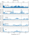 |
Fig. 1 GLS periodogram of IRD and ESPRESSO RVs, and ESPRESSO activity indicators of TOI-521. The vertical grey shows the planetary period of TOI-521.01 at ~1.54. In the ESPRESSO RVs periodogram, the significant peak at f = 0.351 d−1 (~2.85 d) corresponds to the daily alias of the planetary period. The horizontal dashed, dash-dotted, and dotted lines show the 10,1, and 0.1% FAP levels, respectively. |
5 Data analysis and results
5.1 Photometric fit
We performed a photometric fit including all the available data with the PyORBIT9 code (Malavolta et al. 2016, 2018). We detrended the TESS light curves using a biweight time-windowed slider (1-d window) as implemented in WOTAN10 (Hippke et al. 2019), masking the in-transit points to avoid affecting the transit shape11. For each ground-based transit, we included a second-order polynomial to model the out-of-transit variability. We fitted the central time of transit (T0), period (P), stellar radius ratio (Rp/R⋆), impact parameter (b), and stellar density (ρ⋆), adopting a Gaussian prior as derived from the stellar analysis, and limb-darkening (LD) coefficients (q1, q2) as parametrised in Kipping (2013). For each bandpass, we computed the LD coefficients with the PyLDTk12 code (Husser et al. 2013; Parviainen & Aigrain 2015), and we adopted them as Gaussian priors with a custom 0.1 uncertainty. For each light curve, we also included a jitter term to account for uncorrelated noise. For all fitted parameters we adopted uniform priors, if not specified otherwise. We explored the parameter space with the PyORBIT PyDE13 + emcee (Foreman-Mackey et al. 2013) configuration, using the same model specifications and convergence criteria described in Lacedelli et al. (2024).
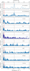 |
Fig. 2 Same as Fig. 1, but for the HARPS and ESPRESSO RVs, and the ESPRESSO activity indicators of TOI-912. The vertical grey and red lines show the planetary signal of TOI-912.01 (~4.7 d) and the stellar rotational period (~46 d). |
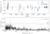 |
Fig. 3 RV residuals and GLS periodogram after the 1-planet (circular) model fit for TOI-521. The vertical dashed line in the periodogram highlights the most significant peak. |
5.2 RV fit
We fitted all the available RVs, testing for each planet with both a circular and an eccentric model with free eccentricity (e)14, comparing the Bayesian evidence (𝒵) through the dynesty nested sampling algorithm (Skilling 2004, 2006; Speagle 2020) as implemented in PyORBIT, adopting a sampling efficiency of 0.3 and 1000 live points. We fitted the RV semi-amplitude (K ∈ [0.01–100] m s−1), the T0 and P (with narrow, uniform priors around the values obtained from the photometric fit), a systemic RV offset (γ), and a jitter term (σj).
For TOI-512 b, the eccentric model was not favoured by the Bayesian evidence, with Δ ln 𝒵 = 0.9 (Kass & Raftery 1995), and the derived eccentricity was unconstrained, and in any case consistent with 0 within 1σ. We therefore assumed the simplest model with a circular orbit. However, the periodogram of the residuals after the one-planet fit showed a significant peak at ~20 d (Fig. 3). Considering also the high jitter of ESPRESSO (σj ~ 3.4 m s−1), we therefore tested a two-planet model, leaving the period of the second candidate free to span between 4 and 200 days. The two-planet model identifies a second signal at P ≃ 20.3 days, with a semi-amplitude of 3.9 ± 0.9 m s−1. This model is favoured by the Bayesian evidence with respect to the one-planet model, with a difference of Δ ln 𝒵 = 2.4. The signal at ~20 days is not identified in any of the activity indicators, and it is inconsistent with the long rotational period suggested from the ![Mathematical equation: $\[\log~ \mathrm{R}_{\mathrm{HK}}^{\prime}\]$](/articles/aa/full_html/2026/01/aa57304-25/aa57304-25-eq11.png) (Sect. 4.2). We therefore associate it with a second candidate in the system, even though further observations will be needed to finally confirm it as a planet, given that the model is statistically favoured, but not strongly. We tested both a circular and an eccentric model for the additional candidate, and we found that the eccentric model was not favoured by the Bayesian evidence, and returned an unconstrained eccentricity, consistent with 0. We therefore assumed as a final model a two-planet system with both planets in circular orbits. We note that adding a second planet in the model did not influence the recovered semi-amplitude of TOI-521 b, which was consistent between the two fits (K =
(Sect. 4.2). We therefore associate it with a second candidate in the system, even though further observations will be needed to finally confirm it as a planet, given that the model is statistically favoured, but not strongly. We tested both a circular and an eccentric model for the additional candidate, and we found that the eccentric model was not favoured by the Bayesian evidence, and returned an unconstrained eccentricity, consistent with 0. We therefore assumed as a final model a two-planet system with both planets in circular orbits. We note that adding a second planet in the model did not influence the recovered semi-amplitude of TOI-521 b, which was consistent between the two fits (K = ![Mathematical equation: $\[5.9_{-1.3}^{+1.2}\]$](/articles/aa/full_html/2026/01/aa57304-25/aa57304-25-eq12.png) and
and ![Mathematical equation: $\[5.7_{-1.0}^{+0.9}\]$](/articles/aa/full_html/2026/01/aa57304-25/aa57304-25-eq13.png) m s−1, respectively).
m s−1, respectively).
For TOI-912, given the results of our frequency analysis (Sect. 4.2), we also included in each fit a GP regression model with a quasi-periodic kernel (Grunblatt et al. 2015) to model the stellar activity, fitting the stellar rotation period (Prot), the characteristics’ decay timescale (Pdec), the coherence scale (w), and the GP amplitude (A) as hyper-parameters. We modelled the RVs and the S-index time series together, in order to better inform the GP (Rajpaul et al. 2015; Barragán et al. 2023). For this planet, the eccentric model (ln 𝒵 = −165.7 ± 0.2) is strongly favoured by the Bayesian evidence with respect to the circular one (ln 𝒵 = −170.6 ± 0.2), with Δ ln 𝒵 = 4.9 (Kass & Raftery 1995). However, given the low number of RV points and the spread of the data, which do not optimally sample the rotation period of the star, we also tested a simpler model fitting the activity with a sinusoidal, to check if the GP model is biasing the eccentricity. In the two-Keplerian model, the eccentricity is consistent with the value obtained from the GP fit (e ~ 0.50 ± 0.05). Such high eccentricity is also obtained from a simpler one-planet eccentric model without GP that we tested, albeit with less significance (e = ![Mathematical equation: $\[0.34_{-0.16}^{+0.14}\]$](/articles/aa/full_html/2026/01/aa57304-25/aa57304-25-eq14.png) ). However, in this one-planet model the RV jitter is unusually high, especially for the ESPRESSO dataset (σj,ESPRESSO = 2.1 m s−1, σj,HARPS = 1.1 m s−1), hinting at the presence of an additional signal, as was expected. This is also reflected in the Bayesian evidence comparison. In fact, the models including a second signal to account for the activity are both favoured, even though only slightly when using a Keplerian (Δ ln 𝒵 = 1.6), while having stronger evidence (Δ ln 𝒵 = 4.9) when using a GP regression. This could be related to the fact that in the two-Keplerian model the period of the second Keplerian is not well defined, showing various peaks in the 43–50 d range. The same happens when applying an uninformed GP only on the RV time series, while such a degeneracy is not present when using a GP model informed with the S-index, which results in a very defined peak at ~46 d. Finally, apart from the uniform prior used in all the previous fits, we also tested different priors for the eccentricity; namely, a half-Gaussian zero-mean prior (Van Eylen et al. 2019), a β function (Kipping 2013), and a truncated Rayleigh function (with σ = 0.2). While all these priors favour low eccentricity, in the GP model the results do not change with respect to the uniform prior when using the β and the Rayleigh function, while the half-Gaussian prior leads to a less significant eccentricity (e = 0.21 ± 0.14), still higher than the initial prior. The same happens with the two-Keplerian model, even though in this case the eccentricity is less significant also for the other two functions, still pointing towards higher values with respect to the initial prior (e =
). However, in this one-planet model the RV jitter is unusually high, especially for the ESPRESSO dataset (σj,ESPRESSO = 2.1 m s−1, σj,HARPS = 1.1 m s−1), hinting at the presence of an additional signal, as was expected. This is also reflected in the Bayesian evidence comparison. In fact, the models including a second signal to account for the activity are both favoured, even though only slightly when using a Keplerian (Δ ln 𝒵 = 1.6), while having stronger evidence (Δ ln 𝒵 = 4.9) when using a GP regression. This could be related to the fact that in the two-Keplerian model the period of the second Keplerian is not well defined, showing various peaks in the 43–50 d range. The same happens when applying an uninformed GP only on the RV time series, while such a degeneracy is not present when using a GP model informed with the S-index, which results in a very defined peak at ~46 d. Finally, apart from the uniform prior used in all the previous fits, we also tested different priors for the eccentricity; namely, a half-Gaussian zero-mean prior (Van Eylen et al. 2019), a β function (Kipping 2013), and a truncated Rayleigh function (with σ = 0.2). While all these priors favour low eccentricity, in the GP model the results do not change with respect to the uniform prior when using the β and the Rayleigh function, while the half-Gaussian prior leads to a less significant eccentricity (e = 0.21 ± 0.14), still higher than the initial prior. The same happens with the two-Keplerian model, even though in this case the eccentricity is less significant also for the other two functions, still pointing towards higher values with respect to the initial prior (e = ![Mathematical equation: $\[0.37_{-0.21}^{+0.14}\]$](/articles/aa/full_html/2026/01/aa57304-25/aa57304-25-eq15.png) and
and ![Mathematical equation: $\[0.15_{-0.08}^{+0.09}\]$](/articles/aa/full_html/2026/01/aa57304-25/aa57304-25-eq16.png) , respectively).
, respectively).
Considering this, and based on the Bayesian evidence, we decided to adopt the one-planet model with free eccentricity and GP modelling informed with the S-index in the following global fit. However, we notice that the results on the eccentricity are somehow dependent on the choice of priors, and that the eccentric model is supported, but not overwhelmingly confirmed, by the Bayesian evidence. More RV observations, possibly optimised to sample the rotational period of the star, will be needed to confirm it. Nonetheless, the recovered semi-amplitude of TOI-912 b was consistent among all models, probing the robustness of the semi-amplitude detection. No additional significant peaks are identified in the periodogram of the residuals after our global fit (see Figure D.1, bottom panel).
5.3 Joint photometric and RV modelling
We performed joint modelling with PyORBIT of all photometric and RV data, fitting the parameters as described in Sects. 5.1 and 5.2. We assumed for each planet as the final model the one derived in Sect. 5.2.
We report in Table 3 the final parameters derived for the two systems under analysis. Figures 4 and 5 report the phase-folded TESS light curve and RVs for the two planets in the TOI-521 system, and Fig. 6 shows the results for TOI-912 b. The ground-based transit models and the global RV models are shown in Figs. A.3 and D.1, respectively.
For TOI-521 b, we inferred a radius of 1.98 ± 0.14 R⊕ and a mass of 5.3 ± 1.0 M⊕ (from K = ![Mathematical equation: $\[5.26_{-0.98}^{+0.95}\]$](/articles/aa/full_html/2026/01/aa57304-25/aa57304-25-eq17.png) m s−1), implying a bulk density of 3.8 ± 1.1 g cm−3. A very similar density (4.0 ± 0.9 g cm−3) is recovered for TOI-912 b, which has an almost identical radius, Rp = 1.93 ± 0.13 R⊕ and Mp = 5.1 ± 0.5 M⊕ (from K =
m s−1), implying a bulk density of 3.8 ± 1.1 g cm−3. A very similar density (4.0 ± 0.9 g cm−3) is recovered for TOI-912 b, which has an almost identical radius, Rp = 1.93 ± 0.13 R⊕ and Mp = 5.1 ± 0.5 M⊕ (from K = ![Mathematical equation: $\[4.29_{-0.37}^{+0.39}\]$](/articles/aa/full_html/2026/01/aa57304-25/aa57304-25-eq18.png) m s−1), as TOI-521 b. For this planet, our model shows a significant eccentricity of e = 0.58 ± 0.02. From our fit, we recovered a rotational period for TOI-912 of
m s−1), as TOI-521 b. For this planet, our model shows a significant eccentricity of e = 0.58 ± 0.02. From our fit, we recovered a rotational period for TOI-912 of ![Mathematical equation: $\[45.9_{-0.2}^{+0.6}\]$](/articles/aa/full_html/2026/01/aa57304-25/aa57304-25-eq19.png) d, consistent with our stellar analysis (Sect. 4.2). Both planets are orbiting at short distance from the host star, with P ~ 1.54 d (TOI-521 b) and ~4.67 d (TOI-912 b), implying equilibrium temperatures of Teq = 794 ± 35 K and 551 ± 27 K, respectively. Moreover, we identify an additional signal in the TOI-521 system at P = 20.3 d, which we associate with a second, possibly non-transiting candidate (see Sect. 5.4) with a minimum mass of Mp sin i =
d, consistent with our stellar analysis (Sect. 4.2). Both planets are orbiting at short distance from the host star, with P ~ 1.54 d (TOI-521 b) and ~4.67 d (TOI-912 b), implying equilibrium temperatures of Teq = 794 ± 35 K and 551 ± 27 K, respectively. Moreover, we identify an additional signal in the TOI-521 system at P = 20.3 d, which we associate with a second, possibly non-transiting candidate (see Sect. 5.4) with a minimum mass of Mp sin i = ![Mathematical equation: $\[10.7_{-2.4}^{+2.5}\]$](/articles/aa/full_html/2026/01/aa57304-25/aa57304-25-eq20.png) M⊕ (from K = 4.5 ± 1.0 m s−1). Due to the presence of this second candidate, we performed a transit time variation (TTV) analysis, to check for possible mutual interactions between the two. Due to its unusually high eccentricity, we performed the same analysis for TOI-912 b, to investigate the presence of additional, non-detected interacting planets in the system. We performed the fit as is described in Sect. 5.1, but leaving each T0 free to vary15, and using the derived eccentricity value for TOI-912 b as a Gaussian prior. As is shown in Fig. E.1, when comparing the observed T0 with the ones calculated from the linear ephemeris (Table 3), we see no significant TTV patterns, with all the computed transit times consistent with the linear ephemeris at 2σ.
M⊕ (from K = 4.5 ± 1.0 m s−1). Due to the presence of this second candidate, we performed a transit time variation (TTV) analysis, to check for possible mutual interactions between the two. Due to its unusually high eccentricity, we performed the same analysis for TOI-912 b, to investigate the presence of additional, non-detected interacting planets in the system. We performed the fit as is described in Sect. 5.1, but leaving each T0 free to vary15, and using the derived eccentricity value for TOI-912 b as a Gaussian prior. As is shown in Fig. E.1, when comparing the observed T0 with the ones calculated from the linear ephemeris (Table 3), we see no significant TTV patterns, with all the computed transit times consistent with the linear ephemeris at 2σ.
5.4 Photometric search and sensitivity limits for TOI-521
Our analysis shows the minimum mass of the additional candidate TOI-521 c is ![Mathematical equation: $\[10.7_{-2.4}^{+2.5}\]$](/articles/aa/full_html/2026/01/aa57304-25/aa57304-25-eq21.png) M⊕. With this mass, we used spright (Parviainen et al. 2024) to compute its most probable radius distribution, finding it likely has a radius of 3.1 R⊕ and a 95% probability of falling between 1.8 and 5.1 R⊕. We searched for this planet in TESS data using the SHERLOCK package (Pozuelos et al. 2020; Dévora-Pajares et al. 2024) but found no signal in the current dataset. We then tested the detectability with the MATRIX code by injecting and recovering synthetic planetary signals, using periods from 18 to 23 days and sizes from 1.5 to 5.5 R⊕ (see e.g. Dévora-Pajares & Pozuelos 2022; Pozuelos et al. 2023). As is shown in Fig. 7, detectability depends strongly on the candidate’s size. The nominal size from spright yields a ~70% recovery rate, increasing to 100% for sizes above 3.5 R⊕. For sizes ≤3.0 R⊕, recovery drops below 10%, indicating that the candidate is undetectable in this range using the available dataset. Thus, we can currently only rule out a transiting body with sizes above 3.5 R⊕ around this period.
M⊕. With this mass, we used spright (Parviainen et al. 2024) to compute its most probable radius distribution, finding it likely has a radius of 3.1 R⊕ and a 95% probability of falling between 1.8 and 5.1 R⊕. We searched for this planet in TESS data using the SHERLOCK package (Pozuelos et al. 2020; Dévora-Pajares et al. 2024) but found no signal in the current dataset. We then tested the detectability with the MATRIX code by injecting and recovering synthetic planetary signals, using periods from 18 to 23 days and sizes from 1.5 to 5.5 R⊕ (see e.g. Dévora-Pajares & Pozuelos 2022; Pozuelos et al. 2023). As is shown in Fig. 7, detectability depends strongly on the candidate’s size. The nominal size from spright yields a ~70% recovery rate, increasing to 100% for sizes above 3.5 R⊕. For sizes ≤3.0 R⊕, recovery drops below 10%, indicating that the candidate is undetectable in this range using the available dataset. Thus, we can currently only rule out a transiting body with sizes above 3.5 R⊕ around this period.
Best-fitting parameters of two systems under analysis.
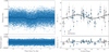 |
Fig. 4 Phase-folded TESS light curve (left) and RVs (right) of TOI-521 b from the joint photometric and RV analysis. The bottom panels show the model residuals. The best-fitting model is plotted as a solid black line. In the transit plot, the black dots show the data binned over 15 min. In the RV plot, the error bars include the jitter term, added in quadrature to the nominal error, and the shaded grey area highlights the ±1σ region. |
6 Discussion
6.1 Mass, radius, and composition
We show in Fig. 8 the position of the two transiting planets in the mass-radius diagram, comparing it with the known, well-characterised population of sub-Neptunes around M dwarfs. Considering the recent results of Leleu et al. (2024), who report that (nearly) resonant sub-Neptunes, which is usually the case for TTV planets, are less dense than non-resonant systems, we removed from the plot all planets flagged as showing TTVs, as they may belong to a separate demographic population.
Interestingly, TOI-521 b and TOI-912 b, which orbit very similar stars (Sect. 4), also have almost identical masses and radii. They are located in the degenerate region of the mass-radius diagram where different internal structures and models can explain their composition. In fact, their planetary density could be consistent with both a significant amount of water in their interiors (up to ~20%, according to (Luo et al. 2024) models including water dissolution in the planetary interiors), or a rocky core plus a ~0.5% H-He envelope (Lopez & Fortney 2014). This degeneracy is further confirmed by the internal structure model that we performed with the ExoMDN16 code (Baumeister & Tosi 2023), which computes through mixture density networks the mass and radius fraction of a fixed four-layer planet (core, mantle, water, and atmosphere) given a planetary mass, radius, and temperature. As Fig. F.1 shows, both planets have high uncertainties on the water content, which could be up to ~40–50% in mass fraction, and a negligible H/He envelope, which can however take up to ~20–25% of the radius fraction. It is important to note that this computation was performed assuming the equilibrium temperature of the planets reported in Table 3, which could not be accurate in the case of TOI-912 b due to tidal heating (see Sect. 6.2), which could imply a more extended envelope.
While the water-world hypothesis (i.e. Luque & Pallé 2022) and atmospheric mass-loss processes (i.e. Rogers et al. 2023) have often been used to explain the distribution and internal composition of this category of sub-Neptunes, more complex models that are currently being developed, including for example redox processes, hydrogen miscibility, magma ocean interactions, and core and mantle melting, will be necessary to properly describe the physical processes happening in the interior and atmospheres of such planets (i.e. Dorn & Lichtenberg 2021; Rogers et al. 2024; Luo et al. 2024; Gupta et al. 2025). However, independently of the adopted internal model, when looking at the current THIRSTEE newly characterised exoplanets around M-dwarfs, which also includes aTOI-406 b, c (Lacedelli et al. 2024) and TOI-771 b (Lacedelli et al. 2025), it seems that this sample supports the hypothesis formulated by Luque & Pallé (2022), according to which sub-Neptunes are divided into at least two distinct density populations, with a density gap around 0.65 ρ⊕,s17 (Fig. 9).
The division of the sub-Neptunes into different populations is also clear when looking at their radius distribution, with planets above the radius gap (Fulton et al. 2017) being mostly volatile-enriched, and planets below the gap being consistent with a rocky composition (Fig. 10). As was expected, both TOI-521 b and TOI-912 b are located above the location of the radius gap for M dwarfs (Van Eylen et al. 2018; Cloutier et al. 2020; Venturini et al. 2024). However, while TOI-912 b is located in a highly populated region of the diagram, TOI-521 b stands up as one of the shortest period sub-Neptunes above, but nearly in the radius gap according to the observational prediction of Van Eylen et al. (2021). This makes it a very interesting target for studying the evolution of planetary atmospheres at short orbital periods, as well as for modelling the interior water mass fraction of highly irradiated planets (i.e. Aguichine et al. 2021).
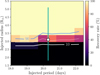 |
Fig. 7 Results of the injection-recovery experiment performed with MATRIX to assess the detectability of the candidate TOI-521 c. The colour scale represents recovery rates, where bright yellow indicates high recovery and dark purple or black indicates low recovery. The solid blue line marks the 90% recovery contour, the dashed white line indicates the 50% one, and the solid white line shows 10%. The white dot marks the nominal value for TOI-521 c derived using spright, and the solid green line denotes the 95% credible interval of the most probable radius distribution. |
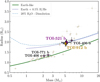 |
Fig. 8 Mass-radius diagram for well-characterised sub-Neptunes around M dwarfs. Data were taken from the PlanetS catalogue (Parc et al. 2024), including also more recently characterised planets from the NASA Exoplanet Archive (as of July 17, 2025), that have radii and masses measured with a precision better than 8% and 25%, respectively. Planets flagged as showing TTVs are removed from sample. The two planets characterised in this work are highlighted with purple and golden diamonds, and the additional planets of the THIRSTEE sample are reported with pink stars. The coloured lines represent different theoretical compositions: the Earth-like composition (solid green line) from (Zeng et al. 2019); Earth-like cores with H/He envelopes at F = 10 F⊕ stellar flux (dotted dark blue line) from Lopez & Fortney (2014); a model including water dissolution in both core and mantle (dotted grey line) from Luo et al. (2024). |
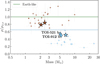 |
Fig. 9 Mass-density of the M-dwarf population of sub-Neptunes, using the same sample as in Fig. 8, adapted from (Luque & Pallé 2022). TOI-912 b and TOI-521 b are labelled and highlighted with diamonds, and the additional THIRSTEE planets are represented with stars. Planets are divided into two populations according to their density, assuming a density gap at 0.65 ρ⊕,s (dotted blue line), which according to Luque & Pallé (2022) divides the population of rocky planets (brown points) from a volatile (or gas-) enriched population (blue points). |
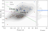 |
Fig. 10 Period-radius diagram of the M-dwarf population of sub-Neptunes, using the same sample as in Fig. 8. Planets are colour-coded according to their density, as in Fig. 9. The green-dashed and purple-dotted lines mark the position of the radius gap for M dwarfs estimated by Van Eylen et al. (2021) and Venturini et al. (2024), respectively. The two planets under analysis are highlighted with diamonds. The blue lines on the histogram, which shows the radius distribution of the sample, marks the radius values of the two targets. |
6.2 Eccentricity of TOI-912 b
While almost identical to TOI-521 b in mass and radius, TOI-912 b is very different in terms of orbital properties. In fact, while for TOI-521 b our model suggests a circular orbit, TOI-912 b has an eccentricity of e = 0.58 ± 0.02, which, if confirmed in the future (see Sect. 5.2), would make it one of the most eccentric sub-Neptunes discovered to date (Fig. 11). Recent discoveries on sub-Neptunes report the presence of similar short-period, eccentric planets, such as TOI-5800 b (Naponiello et al. 2025; Jenkins et al. 2025), which are thought to undergo high-eccentricity migration (HEM) moving into the Neptunian desert. The circularisation timescale, tc (Goldreich & Soter 1966; Rasio et al. 1996), for TOI-912 b, assuming the derived stellar and planetary parameters and a modified tidal quality factor, ![Mathematical equation: $\[Q_{p}^{\prime}\]$](/articles/aa/full_html/2026/01/aa57304-25/aa57304-25-eq60.png) , of 105 (as the one estimated for Uranus and Neptune; Tittemore & Wisdom 1990; Banfield & Murray 1992), is around ~14 Gyr. This is consistent with the HEM scenario, according to which the planet migrated on a highly eccentric orbit, and it is still in the process of tidal circularisation (i.e. Rasio et al. 1996). An alternative explanation could be the presence of an additional, perturbing body in mean motion resonance, which can excite the eccentricity of planet b while maintaining a stable orbital configuration (i.e. Mardling 2007). However, according to our TTV analysis, there is no evidence of such a strongly interacting body in the current dataset. Nonetheless, considering the short observational baseline, additional observations will be essential to investigate the possibility of a currently undetected body. The high eccentricity could also be the result of giant impacts after disc dispersal (Shibata & Izidoro 2025). In this scenario, rocky planets (initially Rp≲ 2 R⊕) that undergo strong dynamical instabilities and numerous late giant impacts have their orbits excited (increased eccentricity) and their radii increased, ultimately placing them into the radius valley. This could explain the higher eccentricity (marginally) observed for planets within the radius valley that has recently been highlighted by Gilbert et al. (2025). With Rp ~ 1.98 R⊕, TOI-912 b seems to follow this trend.
, of 105 (as the one estimated for Uranus and Neptune; Tittemore & Wisdom 1990; Banfield & Murray 1992), is around ~14 Gyr. This is consistent with the HEM scenario, according to which the planet migrated on a highly eccentric orbit, and it is still in the process of tidal circularisation (i.e. Rasio et al. 1996). An alternative explanation could be the presence of an additional, perturbing body in mean motion resonance, which can excite the eccentricity of planet b while maintaining a stable orbital configuration (i.e. Mardling 2007). However, according to our TTV analysis, there is no evidence of such a strongly interacting body in the current dataset. Nonetheless, considering the short observational baseline, additional observations will be essential to investigate the possibility of a currently undetected body. The high eccentricity could also be the result of giant impacts after disc dispersal (Shibata & Izidoro 2025). In this scenario, rocky planets (initially Rp≲ 2 R⊕) that undergo strong dynamical instabilities and numerous late giant impacts have their orbits excited (increased eccentricity) and their radii increased, ultimately placing them into the radius valley. This could explain the higher eccentricity (marginally) observed for planets within the radius valley that has recently been highlighted by Gilbert et al. (2025). With Rp ~ 1.98 R⊕, TOI-912 b seems to follow this trend.
Due to its high eccentricity, tidal dissipation plays an important role in the thermal structure of the planet. We estimated the tidal luminosity of the planet, following Leconte et al. (2010) and assuming ![Mathematical equation: $\[Q_{p}^{\prime}\]$](/articles/aa/full_html/2026/01/aa57304-25/aa57304-25-eq61.png) = 105, to be ~1.97 × 10¹⁷W18. This is almost a few percent of the incident stellar flux received from the host star (~9.8 × 10¹⁸ W), and it therefore implies an important additional internal heating source. This can significantly alter the thermal balance, the internal and atmospheric properties of the planet, and especially the radius inflation in presence of an atmosphere. Given the results of our RV analysis in Sect. 5.2, we stress that additional, well-sampled observations will be needed to definitely confirm the eccentricity of the planet.
= 105, to be ~1.97 × 10¹⁷W18. This is almost a few percent of the incident stellar flux received from the host star (~9.8 × 10¹⁸ W), and it therefore implies an important additional internal heating source. This can significantly alter the thermal balance, the internal and atmospheric properties of the planet, and especially the radius inflation in presence of an atmosphere. Given the results of our RV analysis in Sect. 5.2, we stress that additional, well-sampled observations will be needed to definitely confirm the eccentricity of the planet.
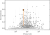 |
Fig. 11 Eccentricity of all known exoplanets with Rp < 4 R⊕ (from the NASA Exoplanet Archive as of 17 July 2025) as a function of orbital period. TOI-912 b is highlighted with an orange diamond. The orange line marks a conservative lower limit to the eccentricity, encompassing all the values of the models discussed in Sect. 5.2. |
6.3 Prospects of atmospheric characterisation
We computed the transmission and emission spectroscopy metrics (TSM and ESM; Kempton et al. 2018) to investigate the suitability of the targets for atmospheric characterisation. With TSM = 83.5 and ESM = 5.4, TOI-912 b is at the lowest limit of the observability thresholds19, making it a suitable candidate for both transmission and emission studies, albeit not an optimal one. However, it is worth noting that both metrics were computed assuming the equilibrium temperature of the planet based only on stellar irradiation, while the planet is likely to have a much higher temperature due to tidal dissipation (see Sect. 6.2), making it a very interesting target also for studying atmospheric mass loss processes. Similarly, TOI-521 b has TSM = 54.1 and ESM = 6.9, making it a suitable target for JWST studies, especially in emission spectroscopy.
Even though they are slightly more massive, TOI-521 b and TOI-912 b have similar properties to GJ 9827 d (Teq~ 618 K, Rp= 1.98 R⊕, Mp= 3.02 M⊕), for which atmospheric features have been recently identified with JWST (Piaulet-Ghorayeb et al. 2024). These planets will therefore be interesting targets to test the compositional trend with temperature suggested by Piaulet-Ghorayeb et al. (2024), hinting at a decrease in the H2-He feature strength from colder to warmer sub-Neptunes.
7 Conclusions
In this work, we have characterised two new sub-Neptunes, TOI-521 b and TOI-912 b, as part of the THIRSTEE sample, using TESS data, ground-based photometry, and high-precision ESPRESSO, HARPS, and IRD RVs. The two planets orbit similar M3 dwarfs and have almost identical radii (1.98 ± 0.14 R⊕; 1.93 ± 0.13 R⊕) and masses (5.3 ± 1.0 M⊕; 5.1 ± 0.5 M⊕), implying a median bulk density of ~4 g cm−3. With such a density, they lie within a highly degenerate region of the mass-radius diagram, where both a volatile-rich and a H/He envelope composition can explain their bulk properties. Even though both planets have short orbital periods (P = 1.5 d and P= 4.7 d, respectively), TOI-521 b has a circular orbit and is located very close to the radius gap line, while TOI-912 b is (likely) one of the most eccentric (e = 0.58 ± 0.02) sub-Neptunes discovered up to date, making it a very interesting target for tidal interaction studies. Finally, we identified a second candidate in a 20.3-d orbit in the TOI-521 system, with a minimum mass of Mp sin i = 10.7 M⊕, which places it between the sub-Neptune and Neptune regime, even though it has currently not been detected in transit. Given the low significance of the model comparison, more observations are needed to confirm it as a planet.
Both TOI-521 b and TOI-912 b add to the sample of well-characterised sub-Neptunes around M-dwarfs, proving the effectiveness of the THIRSTEE programme, and they further strengthen the hypothesis of a density gap among the M-dwarf population (Luque & Pallé 2022; Schulze et al. 2024), as the previous THIRSTEE targets. Finally, these sibling planets are warm sub-Neptunes (Teq= 794 and 551 K), and they are both suitable for atmospheric characterisation studies with JWST, especially in the context of investigating the compositional trends with temperature among the sub-Neptune population.
Data availability
The ESPRESSO, HARPS and IRD RVs and activities indicators are available at the CDS via https://cdsarc.cds.unistra.fr/viz-bin/cat/J/A+A/705/A260.
Acknowledgements
We thank the referee for the comments which improved the quality of this manuscript. We acknowledge financial support from the Agencia Estatal de Investigación of the Ministerio de Ciencia e Innovación MCIN/AEI/10.13039/501100011033 and the ERDF “A way of making Europe” through project PID2021-125627OB-C32, and from the Centre of Excellence “Severo Ochoa” award to the Instituto de Astrofisica de Canarias. We acknowledge funding from the European Research Council under the ERC Grant Agreement n. 337591-ExTrA. This paper includes data collected by the TESS mission, which are publicly available from the Mikulski Archive for Space Telescopes (MAST). Funding for the TESS mission is provided by the NASA Explorer Program. Resources supporting this work were provided by the NASA High-End Computing (HEC) Program through the NASA Advanced Supercomputing (NAS) Division at Ames Research Center for the production of the SPOC data products. We acknowledge the use of public TESS data from pipelines at the TESS Science Office and at the TESS Science Processing Operations Center. This research has made use of the Exoplanet Follow-up Observation Program (ExoFOP; DOI: 10.26134/ExoFOP5) website, which is operated by the California Institute of Technology, under contract with the National Aeronautics and Space Administration under the Exoplanet Exploration Program. Funding for the TESS mission is provided by NASA’s Science Mission Directorate. This research has made extensive use of the SIMBAD database, operated at CDS, Strasbourg, France, and NASA’s Astrophysics Data System. This research has made use of the NASA Exoplanet Archive, which is operated by the California Institute of Technology, under contract with the National Aeronautics and Space Administration under the Exoplanet Exploration Program. This work has made use of data from the European Space Agency (ESA) mission Gaia (https://www.cosmos.esa.int/gaia), processed by the Gaia Data Processing and Analysis Consortium (DPAC, https://www.cosmos.esa.int/web/gaia/dpac/consortium). Funding for the DPAC has been provided by national institutions, in particular the institutions participating in the Gaia Multilateral Agreement. This publication makes use of data products from the Two Micron All Sky Survey, which is a joint project of the University of Massachusetts and the Infrared Processing and Analysis Center/California Institute of Technology, funded by the National Aeronautics and Space Administration and the National Science Foundation. This work makes use of observations from the LCOGT network. Part of the LCOGT telescope time was granted by NOIRLab through the Mid-Scale Innovations Program (MSIP). MSIP is funded by NSF. Some of the observations in this paper made use of the High-Resolution Imaging instrument Zorro and were obtained under Gemini LLP Proposal Number: GN/S-2021A-LP-105. Zorro was funded by the NASA Exoplanet Exploration Program and built at the NASA Ames Research Center by Steve B. Howell, Nic Scott, Elliott P. Horch, and Emmett Quigley. Zorro was mounted on the Gemini South telescope of the international Gemini Observatory, a program of NSF’s OIR Lab, which is managed by the Association of Universities for Research in Astronomy (AURA) under a cooperative agreement with the National Science Foundation. on behalf of the Gemini partnership: the National Science Foundation (United States), National Research Council (Canada), Agencia Nacional de Investigación y Desarrollo (Chile), Ministerio de Ciencia, Tecnología e Innovación (Argentina), Ministério da Ciência, Tecnologia, Inovações e Comunicações (Brazil), and Korea Astronomy and Space Science Institute (Republic of Korea). This research is based on data collected at the Subaru Telescope, which is operated by the National Astronomical Observatory of Japan. We are honored and grateful for the opportunity of observing the Universe from Maunakea, which has the cultural, historical and natural significance in Hawaii. This paper is based on observations with the MuSCAT2 instrument, developed by Astrobiology Center, at Telescopio Carlos Sánchez operated on the island of Tenerife by the IAC in the Spanish Observatorio del Teide. This study was partly supported by the JSPS KAKENHI Grant Numbers JP19KK0082, JP20K14521, JP21K13955, JP21K13987, JP23H00133, JP23H01224, JP23H01227, JP23K17709, JP23K25920, JP23K25923, JP24H00017, JP24H00242, JP24H00248, JP24K00689, JP24K07108, JP24K17082, JP24K17083, JP25H00005, JP25K01061, JP25K17450, JSPS Bilateral Program Number JPJSBP120249910, JSPS Grant-in-Aid for JSPS Fellows Grant Number JP24KJ0241, JP25KJ0091, JP25KJ1036, JP25KJ1040, JST SPRING Grant Number JPMJSP2108. The MEarth Team gratefully acknowledges funding from the David and Lucile Packard Fellowship for Science and Engineering (awarded to D.C.). This material is based upon work supported by NSF under grant AST-1616624, and by NASA under grant No. 80NSSC18K0476 (XRP Program). This work is made possible by a grant from the John Templeton Foundation. The opinions expressed in this publication are those of the authors and do not necessarily reflect the views of the John Templeton Foundation. NASA NHFP — Support for this work was provided by NASA through the NASA Hubble Fellowship grant HST-HF2-51559.001-A awarded by the Space Telescope Science Institute, which is operated by the Association of Universities for Research in Astronomy, Inc., for NASA, under contract NAS5-26555. R.L. acknowledges financial support from the Severo Ochoa grant CEX2021-001131-S funded by MCIN/AEI/10.13039/501100011033. R.L. is funded by the European Union (ERC, THIRSTEE, 101164189). Views and opinions expressed are however those of the author(s) only and do not necessarily reflect those of the European Union or the European Research Council. Neither the European Union nor the granting authority can be held responsible for them. D.J., K.G. and G.N. gratefully acknowledge the Centre of Informatics Tricity Academic Supercomputer and networK (CI TASK, Gdańsk, Poland) for computing resources (grant no. PT01187). The work of HPO has been carried out within the framework of the NCCR PlanetS supported by the Swiss National Science Foundation under grants 51NF40_182901 and 51NF40_205606. N.A-D. acknowledges the support of FONDECYT project 1240916.
References
- Aguichine, A., Mousis, O., Deleuil, M., & Marcq, E. 2021, ApJ, 914, 84 [NASA ADS] [CrossRef] [Google Scholar]
- Allard, F., Homeier, D., & Freytag, B. 2012, Phil. Trans. R. Soc. London Ser. A, 370, 2765 [Google Scholar]
- Aller, A., Lillo-Box, J., Jones, D., Miranda, L. F., & Barceló Forteza, S. 2020, A&A, 635, A128 [NASA ADS] [CrossRef] [EDP Sciences] [Google Scholar]
- Angus, R., Aigrain, S., Foreman-Mackey, D., & McQuillan, A. 2015, MNRAS, 450, 1787 [Google Scholar]
- Astudillo-Defru, N., Forveille, T., Bonfils, X., et al. 2017, A&A, 602, A88 [NASA ADS] [CrossRef] [EDP Sciences] [Google Scholar]
- Bailer-Jones, C. A. L., Rybizki, J., Fouesneau, M., Demleitner, M., & Andrae, R. 2021, VizieR Online Data Catalog: I/352 [Google Scholar]
- Banfield, D., & Murray, N. 1992, Icarus, 99, 390 [NASA ADS] [CrossRef] [Google Scholar]
- Barnes, S. A. 2007, ApJ, 669, 1167 [Google Scholar]
- Barragán, O., Gillen, E., Aigrain, S., et al. 2023, MNRAS, 522, 3458 [CrossRef] [Google Scholar]
- Batalha, N. M., Rowe, J. F., Bryson, S. T., et al. 2013, ApJS, 204, 24 [Google Scholar]
- Baumeister, P., & Tosi, N. 2023, A&A, 676, A106 [NASA ADS] [CrossRef] [EDP Sciences] [Google Scholar]
- Bellm, E. C., Kulkarni, S. R., Graham, M. J., et al. 2019, PASP, 131, 018002 [Google Scholar]
- Benneke, B., Roy, P.-A., Coulombe, L.-P., et al. 2024, arXiv e-prints [arXiv:2403.03325] [Google Scholar]
- Bensby, T., Feltzing, S., & Oey, M. S. 2014, A&A, 562, A71 [NASA ADS] [CrossRef] [EDP Sciences] [Google Scholar]
- Berta, Z. K., Irwin, J., Charbonneau, D., Burke, C. J., & Falco, E. E. 2012, AJ, 144, 145 [Google Scholar]
- Biazzo, K., Bozza, V., Mancini, L., & Sozzetti, A. 2022, Astrophys. Space Sci. Lib., 466, 143 [Google Scholar]
- Bitsch, B., Raymond, S. N., & Izidoro, A. 2019, A&A, 624, A109 [NASA ADS] [CrossRef] [EDP Sciences] [Google Scholar]
- Bonfils, X., Almenara, J. M., Jocou, L., et al. 2015, SPIE Conf. Ser., 9605, 96051L [NASA ADS] [Google Scholar]
- Brown, T. M., Baliber, N., Bianco, F. B., et al. 2013, PASP, 125, 1031 [Google Scholar]
- Burn, R., Schlecker, M., Mordasini, C., et al. 2021, A&A, 656, A72 [NASA ADS] [CrossRef] [EDP Sciences] [Google Scholar]
- Ciardi, D. R., Beichman, C. A., Horch, E. P., & Howell, S. B. 2015, ApJ, 805, 16 [NASA ADS] [CrossRef] [Google Scholar]
- Cifuentes, C., Caballero, J. A., Cortés-Contreras, M., et al. 2020, A&A, 642, A115 [NASA ADS] [CrossRef] [EDP Sciences] [Google Scholar]
- Cloutier, R., Rodriguez, J. E., Irwin, J., et al. 2020, AJ, 160, 22 [NASA ADS] [CrossRef] [Google Scholar]
- Cointepas, M., Almenara, J. M., Bonfils, X., et al. 2021, A&A, 650, A145 [NASA ADS] [CrossRef] [EDP Sciences] [Google Scholar]
- Collins, K. 2019, AAS Meeting Abstracts, 233, 140.05 [NASA ADS] [Google Scholar]
- Collins, K. A., Kielkopf, J. F., Stassun, K. G., & Hessman, F. V. 2017, AJ, 153, 77 [Google Scholar]
- Cutri, R., Wright, E. L., Conrow, T., et al. 2021, AllWISE Data Release [Google Scholar]
- Cutri, R. M., Skrutskie, M. F., van Dyk, S., et al. 2003, VizieR Online Data Catalog: 2246 [Google Scholar]
- Davenport, B., Kempton, E. M. R., Nixon, M. C., et al. 2025, ApJ, 984, L44 [Google Scholar]
- Dévora-Pajares, M., & Pozuelos, F. J. 2022, MATRIX: Multi-phAse Transits Recovery from Injected eXoplanets, Zenodo [Google Scholar]
- Dévora-Pajares, M., Pozuelos, F. J., Thuillier, A., et al. 2024, MNRAS, 532, 4752 [CrossRef] [Google Scholar]
- Dorn, C., & Lichtenberg, T. 2021, ApJ, 922, L4 [NASA ADS] [CrossRef] [Google Scholar]
- Eastman, J., Gaudi, B. S., & Agol, E. 2013, PASP, 125, 83 [Google Scholar]
- Foreman-Mackey, D., Hogg, D. W., Lang, D., & Goodman, J. 2013, PASP, 125, 306 [Google Scholar]
- Fulton, B. J., Petigura, E. A., Howard, A. W., et al. 2017, AJ, 154, 109 [Google Scholar]
- Furlan, E., & Howell, S. B. 2017, AJ, 154, 66 [NASA ADS] [CrossRef] [Google Scholar]
- Furlan, E., & Howell, S. B. 2020, ApJ, 898, 47 [NASA ADS] [CrossRef] [Google Scholar]
- Gaia Collaboration (Vallenari, A., et al.) 2023, A&A, 674, A1 [NASA ADS] [CrossRef] [EDP Sciences] [Google Scholar]
- Gilbert, G. J., Petigura, E. A., & Entrican, P. M. 2025, Proc. Natl. Acad. Sci., 122, e2405295122 [Google Scholar]
- Ginzburg, S., Schlichting, H. E., & Sari, R. 2018, MNRAS, 476, 759 [Google Scholar]
- Goldreich, P., & Soter, S. 1966, Icarus, 5, 375 [Google Scholar]
- Gomes da Silva, J., Figueira, P., Santos, N., & Faria, J. 2018, J. Open Source Softw., 3, 667 [Google Scholar]
- Gomes da Silva, J., Santos, N. C., Adibekyan, V., et al. 2021, A&A, 646, A77 [NASA ADS] [CrossRef] [EDP Sciences] [Google Scholar]
- Grunblatt, S. K., Howard, A. W., & Haywood, R. D. 2015, ApJ, 808, 127 [NASA ADS] [CrossRef] [Google Scholar]
- Gupta, A., & Schlichting, H. E. 2019, MNRAS, 487, 24 [Google Scholar]
- Gupta, A., Stixrude, L., & Schlichting, H. E. 2025, ApJ, 982, L35 [Google Scholar]
- Harakawa, H., Takarada, T., Kasagi, Y., et al. 2022, PASJ, 74, 904 [NASA ADS] [CrossRef] [Google Scholar]
- Hart, K., Shappee, B. J., Hey, D., et al. 2023, arXiv e-prints [arXiv:2304.03791] [Google Scholar]
- Hippke, M., David, T. J., Mulders, G. D., & Heller, R. 2019, AJ, 158, 143 [Google Scholar]
- Hirano, T., Kuzuhara, M., Kotani, T., et al. 2020, PASJ, 72, 93 [Google Scholar]
- Howell, S. B., Everett, M. E., Sherry, W., Horch, E., & Ciardi, D. R. 2011, AJ, 142, 19 [Google Scholar]
- Husser, T.-O., Wende-von Berg, S., Dreizler, S., et al. 2013, A&A, 553, A6 [NASA ADS] [CrossRef] [EDP Sciences] [Google Scholar]
- Ikuta, K., Narita, N., Takarada, T., et al. 2025, PASJ, 77, 1101 [Google Scholar]
- Irwin, J., Irwin, M., Aigrain, S., et al. 2007, MNRAS, 375, 1449 [Google Scholar]
- Irwin, J. M., Berta-Thompson, Z. K., Charbonneau, D., et al. 2015, Cambridge Workshop Cool Stars Stellar Systems Sun, 18, 767 [Google Scholar]
- Ishikawa, H. T., Aoki, W., Hirano, T., et al. 2022, AJ, 163, 72 [NASA ADS] [CrossRef] [Google Scholar]
- Ishikawa, H. T., Aoki, W., Kotani, T., et al. 2020, PASJ, 72, 102 [CrossRef] [Google Scholar]
- Izidoro, A., Schlichting, H. E., Isella, A., et al. 2022, ApJ, 939, L19 [NASA ADS] [CrossRef] [Google Scholar]
- Jenkins, J. M. 2020, Kepler Data Processing Handbook, Kepler Science Document KSCI-19081-003 [Google Scholar]
- Jenkins, J. M., Twicken, J. D., McCauliff, S., et al. 2016, SPIE Conf. Ser., 9913, 1232 [Google Scholar]
- Jenkins, S. A., Vanderburg, A., Sethi, R., et al. 2025, ApJ, 989, L20 [Google Scholar]
- Kass, R. E., & Raftery, A. E. 1995, J. Am. Stat. Assoc., 90, 773 [Google Scholar]
- Kempton, E. M. R., Bean, J. L., Louie, D. R., et al. 2018, PASP, 130, 114401 [Google Scholar]
- Kipping, D. M. 2013, MNRAS, 435, 2152 [Google Scholar]
- Kochanek, C. S., Shappee, B. J., Stanek, K. Z., et al. 2017, PASP, 129, 104502 [Google Scholar]
- Kotani, T., Tamura, M., Nishikawa, J., et al. 2018, SPIE, 10702, 1070211 [Google Scholar]
- Kuzuhara, M., Fukui, A., Livingston, J. H., et al. 2024, ApJ, 967, L21 [Google Scholar]
- Kuzuhara, M., Hirano, T., Kotani, T., et al. 2018, SPIE Conf. Ser., 10702, 1070260 [NASA ADS] [Google Scholar]
- Lacedelli, G., Pallé, E., Davis, Y. T., et al. 2025, A&A, 698, A223 [NASA ADS] [CrossRef] [EDP Sciences] [Google Scholar]
- Lacedelli, G., Pallé, E., Luque, R., et al. 2024, A&A, 692, A238 [NASA ADS] [CrossRef] [EDP Sciences] [Google Scholar]
- Leconte, J., Chabrier, G., Baraffe, I., & Levrard, B. 2010, A&A, 516, A64 [NASA ADS] [CrossRef] [EDP Sciences] [Google Scholar]
- Leggett, S. K., Allard, F., Dahn, C., et al. 2000, ApJ, 535, 965 [NASA ADS] [CrossRef] [Google Scholar]
- Leleu, A., Delisle, J.-B., Burn, R., et al. 2024, A&A, 687, L1 [NASA ADS] [CrossRef] [EDP Sciences] [Google Scholar]
- Lopez, E. D., & Fortney, J. J. 2014, ApJ, 792, 1 [Google Scholar]
- Luhman, K. L. 2018, AJ, 156, 271 [Google Scholar]
- Luo, H., Dorn, C., & Deng, J. 2024, Nat. Astron., 8, 1399 [Google Scholar]
- Luque, R., & Pallé, E. 2022, Science, 377, 1211 [NASA ADS] [CrossRef] [Google Scholar]
- Madhusudhan, N., Sarkar, S., Constantinou, S., et al. 2023, ApJ, 956, L13 [NASA ADS] [CrossRef] [Google Scholar]
- Malavolta, L., Mayo, A. W., Louden, T., et al. 2018, AJ, 155, 107 [NASA ADS] [CrossRef] [Google Scholar]
- Malavolta, L., Nascimbeni, V., Piotto, G., et al. 2016, A&A, 588, A118 [NASA ADS] [CrossRef] [EDP Sciences] [Google Scholar]
- Mamajek, E. E., & Hillenbrand, L. A. 2008, ApJ, 687, 1264 [Google Scholar]
- Mardling, R. A. 2007, MNRAS, 382, 1768 [NASA ADS] [Google Scholar]
- Marfil, E., Tabernero, H. M., Montes, D., et al. 2021, A&A, 656, A162 [NASA ADS] [CrossRef] [EDP Sciences] [Google Scholar]
- Masci, F. J., Laher, R. R., Rusholme, B., et al. 2019, PASP, 131, 018003 [Google Scholar]
- McCully, C., Volgenau, N. H., Harbeck, D.-R., et al. 2018, SPIE Conf. Ser., 10707, 107070K [Google Scholar]
- Misener, W., Schlichting, H. E., & Young, E. D. 2023, MNRAS, 524, 981 [NASA ADS] [CrossRef] [Google Scholar]
- Morris, R. L., Twicken, J. D., Smith, J. C., et al. 2020, Kepler Data Processing Handbook: Photometric Analysis, Kepler Science Document KSCI-19081-003 [Google Scholar]
- Naponiello, L., Vissapragada, S., Bonomo, A. S., et al. 2025, A&A, 701, A79 [NASA ADS] [CrossRef] [EDP Sciences] [Google Scholar]
- Narita, N., Fukui, A., Kusakabe, N., et al. 2019, J. Astron. Teles. Instrum. Syst., 5, 015001 [Google Scholar]
- Nutzman, P., & Charbonneau, D. 2008, PASP, 120, 317 [Google Scholar]
- Owen, J. E., & Wu, Y. 2013, ApJ, 775, 105 [Google Scholar]
- Parc, L., Bouchy, F., Venturini, J., Dorn, C., & Helled, R. 2024, A&A, 688, A59 [NASA ADS] [CrossRef] [EDP Sciences] [Google Scholar]
- Parviainen, H., & Aigrain, S. 2015, MNRAS, 453, 3821 [Google Scholar]
- Parviainen, H., Luque, R., & Palle, E. 2024, MNRAS, 527, 5693 [Google Scholar]
- Parviainen, H., Tingley, B., Deeg, H. J., et al. 2019, A&A, 630, A89 [NASA ADS] [CrossRef] [EDP Sciences] [Google Scholar]
- Pepe, F., Cristiani, S., Rebolo, R., et al. 2021, A&A, 645, A96 [NASA ADS] [CrossRef] [EDP Sciences] [Google Scholar]
- Pepe, F., Mayor, M., Rupprecht, G., et al. 2002, The Messenger, 110, 9 [NASA ADS] [Google Scholar]
- Petigura, E. A., Howard, A. W., & Marcy, G. W. 2013, Proc. Natl. Acad. Sci., 110, 19273 [Google Scholar]
- Piaulet-Ghorayeb, C., Benneke, B., Radica, M., et al. 2024, ApJ, 974, L10 [NASA ADS] [CrossRef] [Google Scholar]
- Plez, B. 2012, Astrophysics Source Code Library [record ascl:1205.004] [Google Scholar]
- Pozuelos, F. J., Suárez, J. C., de Elía, G. C., et al. 2020, A&A, 641, A23 [NASA ADS] [CrossRef] [EDP Sciences] [Google Scholar]
- Pozuelos, F. J., Timmermans, M., Rackham, B. V., et al. 2023, A&A, 672, A70 [NASA ADS] [CrossRef] [EDP Sciences] [Google Scholar]
- Rajpaul, V., Aigrain, S., Osborne, M. A., Reece, S., & Roberts, S. 2015, MNRAS, 452, 2269 [Google Scholar]
- Rasio, F. A., Tout, C. A., Lubow, S. H., & Livio, M. 1996, ApJ, 470, 1187 [Google Scholar]
- Rogers, J. G., Schlichting, H. E., & Owen, J. E. 2023, ApJ, 947, L19 [NASA ADS] [CrossRef] [Google Scholar]
- Rogers, J. G., Schlichting, H. E., & Young, E. D. 2024, ApJ, 970, 47 [NASA ADS] [CrossRef] [Google Scholar]
- Rogers, L. A., & Seager, S. 2010, ApJ, 712, 974 [Google Scholar]
- Ryabchikova, T., Piskunov, N., Kurucz, R. L., et al. 2015, Phys. Scr, 90, 054005 [Google Scholar]
- Santerne, A., Díaz, R. F., Almenara, J. M., et al. 2015, MNRAS, 451, 2337 [Google Scholar]
- Schlichting, H. E., & Young, E. D. 2022, Planet. Sci. J., 3, 127 [NASA ADS] [CrossRef] [Google Scholar]
- Schulze, J. G., Wang, J., Johnson, J. A., et al. 2024, Planet. Sci. J., 5, 71 [NASA ADS] [CrossRef] [Google Scholar]
- Schweitzer, A., Passegger, V. M., Cifuentes, C., et al. 2019, A&A, 625, A68 [NASA ADS] [CrossRef] [EDP Sciences] [Google Scholar]
- Scott, N. J., Howell, S. B., Gnilka, C. L., et al. 2021, Front. Astron. Space Sci., 8, 138 [NASA ADS] [CrossRef] [Google Scholar]
- Shappee, B. J., Prieto, J. L., Grupe, D., et al. 2014, ApJ, 788, 48 [Google Scholar]
- Shibata, S., & Izidoro, A. 2025, ApJ, 986, L25 [Google Scholar]
- Skilling, J. 2004, AIP Conf. Ser., 735, 395 [Google Scholar]
- Skilling, J. 2006, Bayesian Anal., 1, 833 [Google Scholar]
- Smith, J. C., Stumpe, M. C., Van Cleve, J. E., et al. 2012, PASP, 124, 1000 [Google Scholar]
- Speagle, J. S. 2020, MNRAS, 493, 3132 [Google Scholar]
- Stassun, K. G., Oelkers, R. J., Pepper, J., et al. 2018, AJ, 156, 102 [Google Scholar]
- Stumpe, M. C., Smith, J. C., Van Cleve, J. E., et al. 2012, PASP, 124, 985 [Google Scholar]
- Stumpe, M. C., Smith, J. C., Catanzarite, J. H., et al. 2014, PASP, 126, 100 [Google Scholar]
- Suárez Mascareño, A., Rebolo, R., & González Hernández, J. I. 2016, A&A, 595, A12 [Google Scholar]
- Tabernero, H. M., Marfil, E., Montes, D., & González Hernández, J. I. 2022, A&A, 657, A66 [NASA ADS] [CrossRef] [EDP Sciences] [Google Scholar]
- Tamura, M., Suto, H., Nishikawa, J., et al. 2012, SPIE, 8446, 84461T [Google Scholar]
- Tittemore, W. C., & Wisdom, J. 1990, Icarus, 85, 394 [NASA ADS] [CrossRef] [Google Scholar]
- Turbet, M., Bolmont, E., Ehrenreich, D., et al. 2020, A&A, 638, A41 [NASA ADS] [CrossRef] [EDP Sciences] [Google Scholar]
- Twicken, J. D., Chandrasekaran, H., Jenkins, J. M., et al. 2010, SPIE, 7740, 673 [Google Scholar]
- Van Eylen, V., Agentoft, C., Lundkvist, M. S., et al. 2018, MNRAS, 479, 4786 [Google Scholar]
- Van Eylen, V., Albrecht, S., Huang, X., et al. 2019, AJ, 157, 61 [Google Scholar]
- Van Eylen, V., Astudillo-Defru, N., Bonfils, X., et al. 2021, MNRAS, 507, 2154 [NASA ADS] [Google Scholar]
- Venturini, J., Ronco, M. P., Guilera, O. M., et al. 2024, A&A, 686, L9 [NASA ADS] [CrossRef] [EDP Sciences] [Google Scholar]
- Zechmeister, M., & Kürster, M. 2009, A&A, 496, 577 [CrossRef] [EDP Sciences] [Google Scholar]
- Zechmeister, M., Reiners, A., Amado, P. J., et al. 2018, A&A, 609, A12 [NASA ADS] [CrossRef] [EDP Sciences] [Google Scholar]
- Zeng, L., Jacobsen, S. B., Sasselov, D. D., et al. 2019, Proc. Natl. Acad. Sci., 116, 9723 [Google Scholar]
We analysed the SAP photometry to search for the rotational period of the star as the PDCSAP flux is automatically corrected for long-term trends and variability which could remove part of the rotational signal (Smith et al. 2012; Stumpe et al. 2012, 2014).
We compared the results of the detrended data with a fit including a Gaussian process (GP) regression within the model, using a Matérn-3/2 kernel. Given the consistency of the obtained planetary parameters and uncertainties, we decided to adopt the pre-detrended light curves in the global fit to reduce the computational time.
We adopted Eastman et al. (2013) parametrisation [![Mathematical equation: $\[\sqrt{e} ~\sin~ \omega\]$](/articles/aa/full_html/2026/01/aa57304-25/aa57304-25-eq62.png) ,
, ![Mathematical equation: $\[\sqrt{e} ~\cos~ \omega\]$](/articles/aa/full_html/2026/01/aa57304-25/aa57304-25-eq63.png) ], with ω = argument of periastron.
], with ω = argument of periastron.
For the epochs having multiple transits, i.e. due to multi-colour simultaneous photometry with MuSCAT2, we included in the fit a unique transit, selecting the one showing the lowest RMS.
ρ⊕,s is the scaled Earth bulk density, as defined in Luque & Pallé (2022).
This depends strongly on the assumed ![Mathematical equation: $\[Q_{p}^{\prime}\]$](/articles/aa/full_html/2026/01/aa57304-25/aa57304-25-eq64.png) , and it can be even higher considering that Leconte et al. (2010) formulation is an approximation for low-eccentricity orbits.
, and it can be even higher considering that Leconte et al. (2010) formulation is an approximation for low-eccentricity orbits.
Kempton et al. (2018) propose ESM> 7.5, and TSM> 90 for 1.5 <R⊕ Rp< 2.75 R⊕ for optimal target selection.
Appendix A Photometric data
We report here additional analysis and figures related to the photometric data collected for TOI-521 and TOI-912. Figure A.1 shows the TESS field of view of each target, with the photometric aperture used for data extraction.
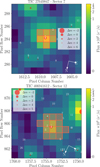 |
Fig. A.1 TPF images of TOI-521 (TIC 27649847, sector 7) and TOI-912 (TIC 406941612, sector 12). In each image, the target star is labelled as 1, and all Gaia DR3 (Gaia Collaboration 2023) sources in the field of view with magnitude contrast up to Δm = 6 are shown with red circles. The photometric aperture used for the light curve extraction is highlighted with red squares. Figures are produced with tpfplotter (Aller et al. 2020). |
Table A.1 summarises the photometric transit data of the planets under analysis, Fig. A.3 shows the results of the ground-based modelling performed in Sect. 5.3.
Additionally, we report the high-resolution speckle imaging we obtained to search for confounding close companions to both stars. The presence of such a companion, whether truly bound or line of sight, provides “third-light” contamination of the observed transit, leading to incorrect derived properties for the exoplanet and its host star (Ciardi et al. 2015; Furlan & Howell 2017, 2020). The stars were observed on 09 December, 2021 (TOI-521) and March 14, 2020 (TOI-912) using the identical speckle instruments, ‘Alopeke and Zorro respectively, mounted on the on the Gemini North/South 8-m telescopes (Scott et al. 2021). Both instruments provide simultaneous speckle imaging in two bands (562 nm and 832 nm were used here) with output data products that include robust 5σ magnitude contrast curves and a reconstructed image. Five sets of 1000 × 0.06 s images were obtained for each star. Data were processed with the standard reduction pipeline (Howell et al. 2011) and Fig. A.2 shows the final 5σ magnitude contrast curves and the 832 nm reconstructed speckle images for both stars. We find that TOI-521 and TOI-912 are both single stars with no companion brighter than 5-6.5 magnitudes and 5-7 magnitudes, respectively, below that of the target star from the Gemini Telescope 8-m telescope diffraction limit (20 mas) out to 1.2 arcsec. At the distance of TOI-521 (d =61 pc) and TOI-912 (d =26 pc), these angular limits correspond to spatial limits of 1.2–73 AU and 0.5-31 AU, respectively.
Summary of the photometric observations for TOI-521 and TOI-912
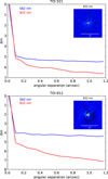 |
Fig. A.2 5σ magnitude contrast curves of the two stars in both filters as a function of the angular separation out to 1.2 arcsec. In each plot, the inset shows the reconstructed 832 nm image with a 1-arcsec scale bar. |
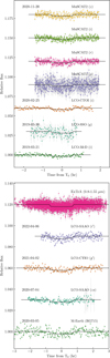 |
Fig. A.3 Ground-based photometry of TOI-521 b (top) and TOI-912 b (bottom). The best-fitting model is plotted as a solid black line. |
Appendix B Stellar analysis
We report here some additional results from our stellar analysis.
Figure B.1 shows the SED fitting of TOI-521 and TOI-912 as described in Sect. 4.1. Figure B.2 shows the position of the two stars in the colour-magnitude diagram of M-dwarfs.
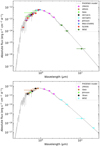 |
Fig. B.1 SED of TOI-521 (top) and TOI-912 (bottom). In both panels, the BT-Settl model computed assuming Teff = 3500 K, log g = 5.0, and solar metallicity is shown with a grey line. |
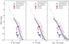 |
Fig. B.2 Color-magnitude diagrams of TOI-521 and TOI-912. The location of main-sequence M-type stars is indicated by the black line, while the grey area accounts for the observed dispersion (Cifuentes et al. 2020). Young stars of the stellar moving Group 29 (Luhman 2018) and old low-metallicity stars of similar colors (Leggett et al. 2000) are also shown for comparison purposes. TOI-521 and TOI-912 appear to be normal main-sequence stars. |
Appendix C Periodogram analysis
We report in Fig. C.1 and C.2 the GLS periodograms of the photometric data analysis for TOI-521 and TOI-912, respectively. Figure C.3 shows the GLS periodogram of the RVs and activity indicators for the IRD dataset (TOI-521) and the HARPS dataset (TOI-912). The stellar rotational period is not identified in any of them. Figure C.4 shows the iterative periodogram of the ESPRESSO RVs for TOI-912.
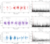 |
Fig. C.1 ASAS-SN (top and middle) and ZTF photometry (bottom) of TOI-521. The light curves are linearly detrended to remove the effect of the high proper motions of the star. The right panel of each plot shows the GLS periodogram, highlighting the 1% (dashed line) and 10% (dotted line) FAP levels. The most significant frequency is marked with a red vertical line. None of the ASAS-SN peaks is highly significant, while for ZTF many peaks and aliases are identified, probably due to the irregular sampling. |
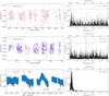 |
Fig. C.2 Same as Fig.C.1, but for the ASAS-SN (top and middle) and TESS SAP (bottom) photometry of TOI-912. The vertical green line shows the possible rotational period of the star. |
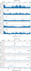 |
Fig. C.3 Same as Fig. 2, but for the IRD dataset of TOI-521 (top) and the HARPS dataset of TOI-912 (bottom). |
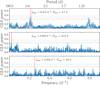 |
Fig. C.4 GLS iterative periodogram of ESPRESSO RVs for TOI-912. At each iteration, the sinusoidal model corresponding to the most significant peak is removed. The second signal identified at ~ 45 d is related to the rotational period of the star (Sect. 4.2). |
Appendix D RV analysis
We report here the results of the global RV modelling of the two stars (Fig. D.1) as performed in Sect. 5.3.
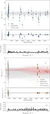 |
Fig. D.1 TOI-521 (top) and TOI-912 (bottom) RV model with residuals from the joint fit. The global model and the GP component are shown with solid grey and red lines, respectively. For each time series, the bottom panel shows the GLS periodogram of the residuals, with the 0.1% and 1% FAP levels shown as horizontal dotted and dashed lines, respectively. |
Appendix E TTV search
We show in Fig. E.1 the results of the TTV analysis of the transiting planets TOI-521 b and TOI-912 b as described in Sect. 5.3.
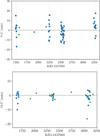 |
Fig. E.1 Observed (O) minus calculated (C) transit times of TOI-521 b. Blue points show the TESS transits, and green triangles mark the ground-based photometric data. For TOI-521 b, due to the shallow depth of the transit, the uncertainties on the T0 of individual TESS transits are considerable. |
Appendix F Internal composition
We show in Fig. F.1 the results of the internal modelling of the planets under analysis performed with ExoMDN.
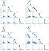 |
Fig. F.1 Radius fraction (left) and mass fraction (right) of the four interior layers of TOI-521 b (top row) and TOI-912 b (bottom row) computed with ExoMDN. |
All Tables
All Figures
|
Fig. 1 GLS periodogram of IRD and ESPRESSO RVs, and ESPRESSO activity indicators of TOI-521. The vertical grey shows the planetary period of TOI-521.01 at ~1.54. In the ESPRESSO RVs periodogram, the significant peak at f = 0.351 d−1 (~2.85 d) corresponds to the daily alias of the planetary period. The horizontal dashed, dash-dotted, and dotted lines show the 10,1, and 0.1% FAP levels, respectively. |
| In the text | |
|
Fig. 2 Same as Fig. 1, but for the HARPS and ESPRESSO RVs, and the ESPRESSO activity indicators of TOI-912. The vertical grey and red lines show the planetary signal of TOI-912.01 (~4.7 d) and the stellar rotational period (~46 d). |
| In the text | |
|
Fig. 3 RV residuals and GLS periodogram after the 1-planet (circular) model fit for TOI-521. The vertical dashed line in the periodogram highlights the most significant peak. |
| In the text | |
|
Fig. 4 Phase-folded TESS light curve (left) and RVs (right) of TOI-521 b from the joint photometric and RV analysis. The bottom panels show the model residuals. The best-fitting model is plotted as a solid black line. In the transit plot, the black dots show the data binned over 15 min. In the RV plot, the error bars include the jitter term, added in quadrature to the nominal error, and the shaded grey area highlights the ±1σ region. |
| In the text | |
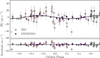 |
Fig. 5 Same as Fig. 4, but showing the phase-folded RVs of the candidate TOI-521 c. |
| In the text | |
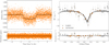 |
Fig. 6 Same as Fig. 4, but for TOI-912 b. |
| In the text | |
|
Fig. 7 Results of the injection-recovery experiment performed with MATRIX to assess the detectability of the candidate TOI-521 c. The colour scale represents recovery rates, where bright yellow indicates high recovery and dark purple or black indicates low recovery. The solid blue line marks the 90% recovery contour, the dashed white line indicates the 50% one, and the solid white line shows 10%. The white dot marks the nominal value for TOI-521 c derived using spright, and the solid green line denotes the 95% credible interval of the most probable radius distribution. |
| In the text | |
|
Fig. 8 Mass-radius diagram for well-characterised sub-Neptunes around M dwarfs. Data were taken from the PlanetS catalogue (Parc et al. 2024), including also more recently characterised planets from the NASA Exoplanet Archive (as of July 17, 2025), that have radii and masses measured with a precision better than 8% and 25%, respectively. Planets flagged as showing TTVs are removed from sample. The two planets characterised in this work are highlighted with purple and golden diamonds, and the additional planets of the THIRSTEE sample are reported with pink stars. The coloured lines represent different theoretical compositions: the Earth-like composition (solid green line) from (Zeng et al. 2019); Earth-like cores with H/He envelopes at F = 10 F⊕ stellar flux (dotted dark blue line) from Lopez & Fortney (2014); a model including water dissolution in both core and mantle (dotted grey line) from Luo et al. (2024). |
| In the text | |
|
Fig. 9 Mass-density of the M-dwarf population of sub-Neptunes, using the same sample as in Fig. 8, adapted from (Luque & Pallé 2022). TOI-912 b and TOI-521 b are labelled and highlighted with diamonds, and the additional THIRSTEE planets are represented with stars. Planets are divided into two populations according to their density, assuming a density gap at 0.65 ρ⊕,s (dotted blue line), which according to Luque & Pallé (2022) divides the population of rocky planets (brown points) from a volatile (or gas-) enriched population (blue points). |
| In the text | |
|
Fig. 10 Period-radius diagram of the M-dwarf population of sub-Neptunes, using the same sample as in Fig. 8. Planets are colour-coded according to their density, as in Fig. 9. The green-dashed and purple-dotted lines mark the position of the radius gap for M dwarfs estimated by Van Eylen et al. (2021) and Venturini et al. (2024), respectively. The two planets under analysis are highlighted with diamonds. The blue lines on the histogram, which shows the radius distribution of the sample, marks the radius values of the two targets. |
| In the text | |
|
Fig. 11 Eccentricity of all known exoplanets with Rp < 4 R⊕ (from the NASA Exoplanet Archive as of 17 July 2025) as a function of orbital period. TOI-912 b is highlighted with an orange diamond. The orange line marks a conservative lower limit to the eccentricity, encompassing all the values of the models discussed in Sect. 5.2. |
| In the text | |
|
Fig. A.1 TPF images of TOI-521 (TIC 27649847, sector 7) and TOI-912 (TIC 406941612, sector 12). In each image, the target star is labelled as 1, and all Gaia DR3 (Gaia Collaboration 2023) sources in the field of view with magnitude contrast up to Δm = 6 are shown with red circles. The photometric aperture used for the light curve extraction is highlighted with red squares. Figures are produced with tpfplotter (Aller et al. 2020). |
| In the text | |
|
Fig. A.2 5σ magnitude contrast curves of the two stars in both filters as a function of the angular separation out to 1.2 arcsec. In each plot, the inset shows the reconstructed 832 nm image with a 1-arcsec scale bar. |
| In the text | |
|
Fig. A.3 Ground-based photometry of TOI-521 b (top) and TOI-912 b (bottom). The best-fitting model is plotted as a solid black line. |
| In the text | |
|
Fig. B.1 SED of TOI-521 (top) and TOI-912 (bottom). In both panels, the BT-Settl model computed assuming Teff = 3500 K, log g = 5.0, and solar metallicity is shown with a grey line. |
| In the text | |
|
Fig. B.2 Color-magnitude diagrams of TOI-521 and TOI-912. The location of main-sequence M-type stars is indicated by the black line, while the grey area accounts for the observed dispersion (Cifuentes et al. 2020). Young stars of the stellar moving Group 29 (Luhman 2018) and old low-metallicity stars of similar colors (Leggett et al. 2000) are also shown for comparison purposes. TOI-521 and TOI-912 appear to be normal main-sequence stars. |
| In the text | |
|
Fig. C.1 ASAS-SN (top and middle) and ZTF photometry (bottom) of TOI-521. The light curves are linearly detrended to remove the effect of the high proper motions of the star. The right panel of each plot shows the GLS periodogram, highlighting the 1% (dashed line) and 10% (dotted line) FAP levels. The most significant frequency is marked with a red vertical line. None of the ASAS-SN peaks is highly significant, while for ZTF many peaks and aliases are identified, probably due to the irregular sampling. |
| In the text | |
|
Fig. C.2 Same as Fig.C.1, but for the ASAS-SN (top and middle) and TESS SAP (bottom) photometry of TOI-912. The vertical green line shows the possible rotational period of the star. |
| In the text | |
|
Fig. C.3 Same as Fig. 2, but for the IRD dataset of TOI-521 (top) and the HARPS dataset of TOI-912 (bottom). |
| In the text | |
|
Fig. C.4 GLS iterative periodogram of ESPRESSO RVs for TOI-912. At each iteration, the sinusoidal model corresponding to the most significant peak is removed. The second signal identified at ~ 45 d is related to the rotational period of the star (Sect. 4.2). |
| In the text | |
|
Fig. D.1 TOI-521 (top) and TOI-912 (bottom) RV model with residuals from the joint fit. The global model and the GP component are shown with solid grey and red lines, respectively. For each time series, the bottom panel shows the GLS periodogram of the residuals, with the 0.1% and 1% FAP levels shown as horizontal dotted and dashed lines, respectively. |
| In the text | |
|
Fig. E.1 Observed (O) minus calculated (C) transit times of TOI-521 b. Blue points show the TESS transits, and green triangles mark the ground-based photometric data. For TOI-521 b, due to the shallow depth of the transit, the uncertainties on the T0 of individual TESS transits are considerable. |
| In the text | |
|
Fig. F.1 Radius fraction (left) and mass fraction (right) of the four interior layers of TOI-521 b (top row) and TOI-912 b (bottom row) computed with ExoMDN. |
| In the text | |
Current usage metrics show cumulative count of Article Views (full-text article views including HTML views, PDF and ePub downloads, according to the available data) and Abstracts Views on Vision4Press platform.
Data correspond to usage on the plateform after 2015. The current usage metrics is available 48-96 hours after online publication and is updated daily on week days.
Initial download of the metrics may take a while.