| Issue |
A&A
Volume 706, February 2026
|
|
|---|---|---|
| Article Number | A324 | |
| Number of page(s) | 22 | |
| Section | Extragalactic astronomy | |
| DOI | https://doi.org/10.1051/0004-6361/202452051 | |
| Published online | 17 February 2026 | |
Back from the dead: AT2019aalc as a candidate repeating tidal disruption event in an active galactic nucleus
1
Ruhr University Bochum, Faculty of Physics and Astronomy, Astronomical Institute (AIRUB) Universitätsstraße 150 44801 Bochum, Germany
2
Ruhr Astroparticle and Plasma Physics Center (RAPP Center) 44801 Bochum, Germany
3
Leiden Observatory, Leiden University Postbus 9513 2300 RA Leiden, The Netherlands
4
Deutsches Elektronen-Synchrotron (DESY) Platanenallee 6 D-15378 Zeuthen, Germany
5
Institut fur Physik, Humboldt-Universität zu Berlin D-12489 Berlin, Germany
6
Division of Physics, Mathematics, and Astronomy, California Institute of Technology Pasadena CA 91125, USA
7
University of Maryland, Department of Astronomy 4296 Stadium Dr College Park MD 20742, USA
8
NASA Goddard Space Flight Center, Astrophysics Science Division 8800 Greenbelt Rd Greenbelt MD 20771, USA
9
Center for Research and Exploration in Space Science and Technology, NASA/GSFC Greenbelt MD 20771, USA
10
Department of Particle Physics and Astrophysics, Weizmann Institute of Science 76100 Rehovot, Israel
11
Cahill Center for Astrophysics, California Institute of Technology, MC 249-17 1200 E California Boulevard Pasadena CA 91125, USA
★ Corresponding author: This email address is being protected from spambots. You need JavaScript enabled to view it.
Received:
29
August
2024
Accepted:
21
November
2025
Abstract
Context. To date, three nuclear transients have been associated with high-energy neutrino events. These transients are generally thought to be powered by tidal disruption events (TDEs) in stars caused by massive black holes. However, AT2019aalc, hosted in a Seyfert-1 galaxy, has not yet been classified due to a lack of multiwavelength observations. Interestingly, the source re-brightened 4 years after its discovery.
Aims. Our aim is to constrain the physical mechanism responsible for the second optical flare, which may also provide clues to the origin of the initial event.
Methods. We conducted a multiwavelength monitoring program (from radio to X-rays) of AT2019aalc during its re-brightening in 2023–2024.
Results. The observations revealed multiple X-ray flares during the second optical flaring episode of the transient and a uniquely bright UV counterpart. The second flare, similar to the first one, is accompanied by IR dust echo emission. A long-term radio flare was found with an inverted spectrum. Optical spectroscopic observations revealed the presence of Bowen fluorescence lines and strong high-ionization coronal lines, indicating an extreme level of ionization in the system.
Conclusions. The results suggest that the transient can be classified as a Bowen fluorescence flare (BFF), a relatively new sub-class of flaring active galactic nuclei (AGNs). AT2019aalc can be also classified as an extreme coronal line emitter (ECLE). We find that in addition to AT2019aalc, another BFF, AT2021loi, is spatially coincident with a high-energy neutrino event. We propose a repeating TDE scenario within an AGN framework to explain the multiwavelength properties of AT2019aalc and suggest a possible connection among ECLEs, BFFs, and TDEs occurring in AGNs.
Key words: neutrinos / galaxies: active / galaxies: individual: AT2019aalc / quasars: emission lines / galaxies: Seyfert / radio continuum: galaxies
© The Authors 2026
 Open Access article, published by EDP Sciences, under the terms of the Creative Commons Attribution License (https://creativecommons.org/licenses/by/4.0), which permits unrestricted use, distribution, and reproduction in any medium, provided the original work is properly cited.
This article is published in open access under the Subscribe to Open model. This email address is being protected from spambots. You need JavaScript enabled to view it. to support open access publication.
1. Introduction
Tidal disruption events (TDEs) are rare transient events that occur when a star approaches a supermassive black hole (SMBH) and the tidal forces of the latter rip the star apart (Rees 1988). As a result, about half of the star’s material is accreted around the black hole, generating a luminous outburst across the electromagnetic spectrum. TDE optical light curves typically exhibit a rapid, colorless rise followed by a fast decay on monthly timescales. Several TDEs have been detected in X-rays, with soft spectra typically explained by late-time accretion disk formation (Saxton et al. 2020). In addition, a handful of TDEs produced detectable radio emission, explained either by delayed1 non-relativistic outflows (Horesh et al. 2021; Cendes et al. 2024) or, only in four instances, by newly launched relativistic on-axis jets (Berger et al. 2012; Brown et al. 2015; Cenko et al. 2012; De Colle & Lu 2020; Yao et al. 2024). Spectroscopically, TDEs are characterized by a strong blue continuum and broad emission lines (> 104 km s−1), such as Hα and Hβ. In a few cases, Bowen fluorescence (BF; Bowen 1934, 1935) lines, such as N III at 4640 Å, appear (e.g., Blagorodnova et al. 2019; Charalampopoulos et al. 2022).
Tidal disruption events generally produce one optical flare. However, in a few cases, a re-brightening episode was detected – even years after the initial flare. These might be explained in the following way. A star on a grazing orbit might be partially disrupted, and only a fraction of the stellar mass will be deposited onto the SMBH. The secondary disruption of a surviving core after it reaches the pericenter again results in re-brightening. This scenario is naturally explained by the Hills capture mechanism (Hills 1988), where a binary star system is disrupted by the SMBH, capturing one star on a highly eccentric orbit prone to repeated partial disruptions. In this process, the captured star’s orbit brings it close enough to the SMBH multiple times, causing episodic stripping of stellar material and producing recurring flares over timescales of months to years. Only a few partial TDEs or candidates are known to date. They are AT2020vdq (Somalwar et al. 2025b), ASASSN−14ko (Payne et al. 2021; Tucker et al. 2021; Payne et al. 2022; Huang et al. 2023), eRASSt J045650.3−203750 (Liu et al. 2023, 2024), RX J133157.6-324319.7 (Hampel et al. 2022), AT2018fyk (Wevers et al. 2019, 2023; Wen et al. 2024; Pasham et al. 2024), AT2019avd (Malyali et al. 2021; Frederick et al. 2021; Chen et al. 2022; Wang et al. 2023, 2024), AT2019azh (Hinkle et al. 2021), AT2022dbl (Lin et al. 2024; Hinkle et al. 2024a; Makrygianni et al. 2025), and AT2021aeuk (Sun et al. 2025).
Based on the observed properties of TDE host galaxies, van Velzen & Farrar (2014) estimated a TDE rate of a few times 10−5 per year per galaxy, which is well borne out by recent data (Yao et al. 2023) and earlier observational estimates (Syer & Ulmer 1999). Importantly, a similar fraction of TDEs should occur in AGN hosts (e.g., Chan et al. 2019; Ryu et al. 2024). These transients are challenging to distinguish from regular AGN variability and only a few candidate TDEs occurring in AGNs (i.e., TDE-AGNs) have been studied earlier – for example, PS16dtm, a TDE in a narrow-line Seyfert-1 (NLSy1) galaxy (Blanchard et al. 2017) and the multiple soft X-ray flares in IC 3599 (Campana et al. 2015) and GSN 069 (Shu et al. 2018). In contrast with the TDEs seen in earlier quiescent galaxies, these transients are characterized by slowly decaying optical emission, and bumps tend to appear after the peak. It is worth noting that transients classified as ambiguous nuclear transients (ANTs; e.g., Wiseman et al. (2025)), as well as several of the events studied by Frederick et al. (2021), could also be TDEs in AGN hosts, potentially increasing their overall number.
Recently, Trakhtenbrot et al. (2019) identified a new class of spectroscopically unique flares from accreting SMBHs. In 2019, the transient events AT2017bgt, F01004-2237, and OGLE17aaj were identified as the first members of the class based on their unique optical spectroscopic features. Later, the peculiar X-ray transient AT2019avd (Malyali et al. 2021; Frederick et al. 2021; Chen et al. 2022; Wang et al. 2023, 2024) was found with remarkably similar properties; however, its classification as an AT2017bgt-like transient is unclear. A more promising case is AT2021loi (Makrygianni et al. 2023), a UV-bright transient event with very similar multiwavelength properties to the three flares studied by Trakhtenbrot et al. (2019). These events show unobscured AGN-like optical spectra with significant and persistent BF lines, a high UV-to-optical ratio, and optical emission that decays on yearly timescales. These AGNs are characterized by accretion that intensifies significantly over long timescales. Hereafter, we refer to this new class of SMBH flares as BF flares (BFFs), following Makrygianni et al. (2023). Using the Zwicky Transient Facility (ZTF; Masci et al. 2019) public survey data, Dgany et al. (2023) found only one BFF candidate (AT2021seu) among 223 spectroscopically classified transients, suggesting that these flares are rare. Two other candidates, namely AT2022fpx, Koljonen et al. (2024) and AT2020afhd Arcavi et al. (2024), were found later.
In recent years, two nuclear transients were found to be spatially coincident with neutrino events detected by the IceCube Neutrino Observatory based on ZTF follow-up campaigns of IceCube neutrino alerts (Stein et al. 2023). The TDE AT2019dsg is likely associated with the neutrino IC191001A (Stein et al. 2021), and a further promising association between the candidate TDE AT2019fdr and IC200530A (Reusch et al. 2022) points to TDEs as a potential new class of sources of the extragalactic neutrinos. Both sources were identified as having luminous mid-infrared emission, and a search for similar flares (van Velzen et al. 2024) led to the identification of the transient event AT2019aalc (also known as ZTF19aaejtoy) with the neutrino alert IC191119A. In addition, two candidate obscured TDEs (Jiang et al. 2023) and the extremely energetic candidate TDE AT2021lwx (Yuan et al. 2024) were associated with high-energy neutrinos. A recently claimed association between a neutrino flare detected by the IceCube Observatory and an X-ray flare from the TDE ATLAS17jrp suggests that the X-ray emission of these sources plays a crucial role in producing neutrinos (Li et al. 2024).
In this paper, we focus on the nuclear transient event and neutrino source candidate AT2019aalc, especially on the significant optical re-brightening that started 4 years after its initial flare (Veres et al. 2023). The paper is organized as follows. We discuss the discovery of the transient event and give insight about its host galaxy in Sect. 2. We summarize our observing campaign and the data reduction in Sect. 3. We present the results of the observations in Sect. 4, discuss them in Sect. 5, and give a final summary and conclude in Sect. 6. Throughout the paper, we adopt a flat Λ cold dark matter cosmological model with parameters H0 = 70 km s−1 Mpc−1, ΩΛ = 0.73, and Ωm = 0.27. In this model (Wright 2006), a 1 mas angular size corresponds to 0.72 pc projected linear size at the source redshift z = 0.0356 (Ahn et al. 2012). This redshift corresponds to a luminosity distance of 158.3 Mpc. All magnitudes are given in the AB system (Oke 1974) unless stated otherwise.
2. The transient event: AT2019aalc
An analysis of the infrared properties of AT2019dsg and AT2019fdr revealed a strong reverberation signal, particularly an the infrared dust echo, stemming from reprocessed emission of optical/UV photons to the infrared by interaction with hot dust around the SMBH, at a distance of 0.1–1 pc (Jiang et al. 2016; Dou et al. 2016; Lu et al. 2016; van Velzen et al. 2021b; Jiang et al. 2021; van Velzen et al. 2024). In addition to the exceptionally high infrared luminosities of these transients, the neutrino detection times appear to be temporally consistent with the infrared luminosity peaks (Stein et al. 2021; Reusch et al. 2022). This discovery motivated a systematic search for neutrino emission using an extended sample of black hole flares (van Velzen et al. 2024). This archival search revealed the nuclear transient AT2019aalc, with a powerful optical flare and dust echo emission in spatial coincidence with the high-energy neutrino event, IC191119A (IceCube Collaboration 2019), detected by the IceCube Observatory.
The host galaxy of AT2019aalc (2MASX J15241665+0451192) is a barred spiral (SBa) galaxy hosting an active nucleus 2013AJ....146..151O. Based on its Sloan Digital Sky Survey (SDSS: Abazajian et al. 2009) spectrum it was further classified as a broad-line Seyfert-1 galaxy (Trump et al. 2013; Liu et al. 2019). The galaxy was detected in archival radio sky surveys e.g., the Very Large Array Faint Images of the Radio Sky at Twenty-cm (VLA FIRST: Condon et al. 1998). Fig. 1 shows the Pan-STARRS (Chambers et al. 2016) i-band optical image of the galaxy, together with the contours of the FIRST radio data (at 1.4 GHz) and the position of the X-ray counterpart detected by the Swift/XRT in 2023–2024. The galaxy is not present in any X-ray catalogs prior to the optical discovery of the transient in 2019. In addition to the significant IR echo, AT2019aalc shares multiwavelength characteristics with the two other neutrino candidate transients: a soft X-ray spectrum and transient radio emission (van Velzen et al. 2024). Moreover, similarly to the other two instances, the infrared peak of the transient event is temporarily coincident with the detection time of the likely associated neutrino event. Notably, Winter & Lunardini (2023) estimated the highest neutrino fluence for AT2019aalc among the studied candidates, due to its high estimated SMBH mass (MBH = 107.2 M⊙, van Velzen et al. 2024) and low redshift. Since the proposed association with the high-energy neutrino event was announced roughly two years after the discovery of the transient event, the source was not at the focus of attention. Thus, the lack of spectroscopic monitoring during the first optical flare hindered a clear classification of the event. Nevertheless, out of the more than 104 AGNs detected by the ZTF, fewer than 1% show similarly rapid and large outbursts (Reusch et al. 2022; van Velzen et al. 2024), suggesting a very unusual transient. Interestingly, roughly 4 years after the first flare, a significant optical re-brightening started in mid-May 2023 (Veres et al. 2023), illustrated by the long-term ZTF difference light curve shown in Fig. 2.
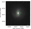 |
Fig. 1. Pan-STARRS i-band pre-flare image centered on the host galaxy position of the transient event AT2019aalc. The object located to the west of the galaxy core is a foreground star. The green contours represent the pre-flare FIRST radio observations taken at 1.4 GHz. The lowest contour level is drawn at 3σ image noise level corresponding to 0.4 mJy beam−1. Additional positive contour levels increase by a factor of two. The peak brightness is 5.8 mJy beam−1. The red circle points to the Swift-XRT 0.3–10 keV astrometrically corrected position of AT2019aalc, determined using the Swift-XRT data products generator (Evans et al. 2014). Its size indicates the 90% confidence positional error. |
3. Observations and data reduction
3.1. Optical/UV
3.1.1. ZTF
ZTF forced photometry at the location of AT2019aalc was obtained following the recommendations outlined in Masci et al. (2019). We corrected for extinction by adopting a galactic extinction of E(B − V) = 0.039 (Schlafly & Finkbeiner 2011). As shown in Fig. 2, the forced photometry yields a negative flux in the period between the two flares (and also just before the first flare). This implies that during these epochs, the flux decreased below the mean flux of the reference images. For the r-band, these were obtained between March 2018 and May 2018. While the baseline used to obtain the difference flux of the g-band is based on images obtained between March and September, 2018.
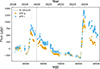 |
Fig. 2. Optical light curve of AT2019aalc derived from ZTF difference photometry. The transparent markers indicate negative flux (i.e., the flux decreased below the mean flux of the reference images). Two distinct flares can be seen. The second flare peaked 4 years after the first one. The blue vertical line indicates the arrival time of the neutrino event IC191119A associated with the transient. |
3.1.2. UVOT
The Neil Gehrels Swift Observatory (Gehrels et al. 2004) performed 33 Target of Opportunity (ToO) observations (project codes: 18972, 19188, 19993, 20997 and 21692, Proposers: Reusch, Veres & Sniegowska) on AT2019aalc from 2023-06-23 to 2025-01-02 with a total exposure time of ≈55 ks. The Ultraviolet and Optical Telescope (UVOT, Roming et al. 2005) onboard the satellite observed the target field with the following four filters in each epoch: UVW2 (central wavelength, 1928 Å), UVM2 (2246 Å), UVW1 (2600 Å) and U (3465 Å). We analyzed the UVOT images using the Swift/UVOT tools included in the HEASOFT 6.30 software package. We measured the flux using UVOTSOURCE, applying a circular aperture of 15 arcseconds (which captures nearly all the flux of the host galaxy). The background was measured using four 6 arcsecond regions in four quadrants away from the target source. To estimate the UV flux before the flare, we use GALEX (Martin et al. 2005) observations obtained in 2007 and 2011. We use the same 15″ circular aperture that was applied to the Swift/UVOT observations and use the GPHOTON software (Million et al. 2016) to extract the flux. Over the four year baseline of the GALEX observations, the NUV magnitudes change by about 0.3 mag. Following van Velzen et al. (2021a), we combine the mean GALEX flux with the SDSS (York et al. 2000) magnitudes and apply Prospector (Johnson & Leja 2017) to find the best-fit stellar population synthesis model (Conroy et al. 2009) that describes these data. From this model we estimate the baseline flux in the UVOT filters and this baseline is subtracted to obtain the difference flux. The baseline flux in the UVM2 band is 17.2 mag, implying an increase of 1.8 mag relative to the peak of the UVM2 light curve. This large increase implies that, at the peak of the flare, we are not sensitive to the value of the baseline flux. This is useful because the baseline of the ZTF forced photometry was obtained around 2018 (at the start of the ZTF survey), while the baseline that is used to obtain the UVOT difference flux is mainly determined by the GALEX observations that were obtained a decade earlier.
3.2. Infrared
The Palomar 200-inch (P200) near-infrared telescope equipped with the Wide Field Infrared Camera (WIRC, Wilson et al. 2003) observed AT2019aalc on 2023-07-05. The imaging was obtained in the J-, H-, and Ks-bands. The data was processed with the SWARP software (Bertin et al. 2002). We performed background subtraction using the PHOTUTILS.BACKGROUND class and measured the flux using a circular aperture with a radius of 9 pixels. The corresponding zero-point magnitudes for this aperture size were calculated using the automatic pipeline for each filter. The error bars are the computed Poisson and background error of the photometry2 and we also took into account the uncertainty of the derived zero-point magnitudes.
We obtained mid-infrared photometry from archival observations of the Wide-Field Survey Explorer (WISE, Wright et al. 2010), which was continuously monitoring the sky at 3.4 μm (W1) and, due to the NEOWISE project (Mainzer et al. 2011), at 4.6 μm (W2). NEOWISE visits any point in the sky roughly every six months, with each visit consisting of about ten exposures. Using timewise (Necker & Mechbal 2024; Necker et al. 2025), we downloaded all available multi-epoch photometry data from the AllWISE data release and single-epoch photometry from the NEOWISE-R data releases and stacked the data per visit to obtain robust measurements. All selected single-exposure photometry data points are within 1 arcsecond of the nucleus of the host. The resulting light curve spans almost 14 years, starting in February 2010 until July 2024.
3.3. X-ray
The X-ray Telescope (XRT, Burrows et al. 2005) observations, in the energy range of 0.3–10 keV, were obtained simultaneously with the UVOT observations. The observations were performed in photon counting mode. We performed the data reduction using the Space Science Data Center interactive archive in the following way: First, cleaned event-files were produced using the XRTPIPELINE and XRTEXPOMAP tasks. The XIMAGE tool allowed us to determine the source detection level and its position. In case of non-detections, 3σ upper limits for the count rate were derived and converted to flux using WebPIMMS3 and assuming the mean power-law index of the observations that resulted in detections. When our target source was detected above the 3σ level, we ran SWXRTDAS in order to extract the source and the background spectra. Source counts were retrieved from a circle with a radius of 20 pixel (47 arcseconds), while background counts were extracted using an annular region with 80/120 pixel inner/outer radius. Finally, the GRPPHA tool of the HEASOFT 6.32 software package was used to perform background subtraction using the source and background spectra. We binned each spectrum to have a minimum of 3 counts per spectral bin.
We fit the individual X-ray spectra using the XSPEC fitting environment (Arnaud 1996). First, we have determined the Galactic neutral hydrogen column density, NH, based on the HI4PI survey (HI4PI Collaboration 2016). The spectrum was then fit using Cash-statistic (C-stat, Cash 1976). To find the best-fitting model, we first fit the stacked spectrum with a absorbed power-law (TBABS*POWERLAW in XSPEC) model, as the last XMM data of AT2019aalc before our monitoring program was best-fit with a power-law model (Pasham 2023). When fitting the model, the galactic column density was fixed whilst the power-law index and the normalization were free to vary. The resultant fit quality is C-Stat = 183.3 for 165 degrees of freedom. We then added a blackbody model component, to take into account a possible soft excess. The blackbody temperature and the normalization of the new component were also free to vary. We fit again, which resulted in a better fit with C-Stat = 170.5 for 163 degrees of freedom. We implemented the likelihood ratio test (lrt in XSPEC) to estimate the statistical significance of the inclusion of the blackbody component. After running 100 simulations, the test resulted only in smaller likelihood differences than the observed one, clearly implying that the difference is unlikely to be due to random fluctuations. Therefore, accounting for the soft X-ray excess results in a significantly better fit.
3.4. Radio
3.4.1. VLBI observations
We observed AT2019aalc with the European VLBI Network (EVN) and the enhanced Multi-Element Remotely Linked Interferometer Network (e-MERLIN, Garrington et al. 2004). These observations were carried out at 1.7 GHz (L-band) on 2023 June 09 (project code: EV027, PI: Veres). The observation time was 10 h. The experiment was performed in phase-referencing mode with 5-min duty cycles (with spending 3.5 min on the target during each cycle) which resulted in an on-source time of 6.7 h including fringe-finder scans and slewing. The data were recorded in left and right circular polarizations with a data rate of 1 Gbit s−1. The correlation was done at the EVN Data Processor (Keimpema et al. 2015) at the Joint Institute for VLBI European Research Infrastructure Consortium (Dwingeloo, The Netherlands) with an averaging time of 2 s. The Compact Symmetric Object (CSO) 1521+0430 (a.k.a. 4C 04.51) at an angular distance of 0.83° was observed as phase-reference calibrator.
The data were calibrated with the U.S. National Radio Astronomy Observatory Astronomical Image Processing System (AIPS, Greisen 1990) software package. The standard procedures including time flagging, amplitude calibration, correction for the dispersive ionospheric delays and global fringe-fitting of the calibrator sources were followed. We imaged the phase-calibrator with the DIFMAP software (Shepherd et al. 1994), using the hybrid mapping technique (Högbom 1974). Using the CLEAN component (CC) model we built up in DIFMAP, we repeated the fringe-fitting in AIPS for the phase-reference calibrator source to correct its structure. Finally, we interpolated the solutions of the last fringe-fitting to the data of our target source. We imaged the target source using the hybrid mapping technique in DIFMAP. At the end of the procedure, several steps of amplitude and phase self-calibration were performed. A simple elliptical Gaussian modelfit component (Pearson 1995) was fit directly to the visibility data. Finally, to decrease the noise level, we performed 1000 CLEAN iterations in the residual image with a small loop gain of 0.01.
3.4.2. ATCA monitoring
The Australia Telescope Compact Array (ATCA)4, located at Narrabri, New South Wales, Australia, was used to monitor AT2019aalc. The observations were conducted between 2023-06-28 and 2024-05-04, utilizing the array in the 6km (6A and 6D) and (H168) configuration. The observations were conducted at frequencies of 2.1 GHz, 5.5 GHz, 9 GHz, 17 GHz and 19 GHz. The flux calibrator was the standard ATCA primary calibrator, 1934–638, and 1548+056 was used as phase calibrator. The observations are summarized in Table 1.
Summary of the ATCA radio continuum emission observations of AT2019aalc.
The data reduction procedures were based on the Multichannel Image Reconstruction, Imaging Analysis and Display (miriad: Sault et al. 1995). The data reduction procedure was conducted in accordance with standard protocols. In order to mitigate the impact of radio frequency interference (RFI) during flux and phase calibration, the interactive flagging tool bflag was utilized. Furthermore, automated flagging routines pgflag were applied to address interference for the source. Any corrupted data identified during calibration was manually flagged.
Due to the limited (u, v)-coverage and the low elevation of the source, which resulted in a very elongated beamshape, we were not able to perform self-calibration and cleaning. Fortunately, AT2019aalc always dominated the flux within the resolution elements of our short observations. Therefore, we imaged the region around our source for each observation using an oversampling of the synthesised beam by a factor of at least 10. Under the assumption that AT2019aalc is always a point-source, we can take the highest pixel value in the image as our measured flux. Due to the uncertainties this method introduced, we used a plain 10% flux error.
3.5. Spectroscopic observations
We observed the spectrum of AT2019aalc on 2021-07-06 using the Low Resolution Imaging Spectrograph (LRIS: Oke et al. 1995) mounted on the Keck-I telescope at Maunakea (PI: Kulkarni). Later, during the second optical flare, we obtained five more optical spectra of AT2019aalc using the following instruments: LRIS (PI: Kulkarni), DeVeny Spectrograph mounted on the Lowell Discovery Telescope (LDT) in Arizona (PI: Hammerstein) and the Double Beam Spectrograph (DBSP, Oke & Gunn 1982) mounted on the 200 inch telescope at Palomar Observatory, California (PIs: Kulkarni and Kasliwal). The spectra were reduced following the standard procedures using the automated reduction pipeline of the LRIS (Perley 2019), the software package PYPEIT (Prochaska et al. 2020) for DeVeny, and the software packages DBSP DRT (Mandigo-Stoba et al. 2022) and PYPEIT (Prochaska et al. 2020) for the DBSP. Details of these observations of AT2019aalc are summarized in Table A.1 while the spectra are shown in Fig. A.1.
To determine the type of AGN prior to the flares, we performed a stellar population synthesis fit of the pre-flare SDSS spectrum with (PPXF: Cappellari & Emsellem 2004; Cappellari 2017, 2023) and the newest GALAXEV (Bruzual & Charlot 2003) models (CB2019), assuming a Kroupa (2001) initial mass function (IMF) and an upper mass limit of 100, as templates (see Fig. A.2). Beforehand, the spectrum was corrected for Milky Way extinction using the dust reddening maps by Schlafly & Finkbeiner (2011) and the Cardelli et al. (1989) extinction curve. Furthermore, it was redshift corrected and logarithmically rebinned. We included several emission lines in the fit and assumed four kinematic components: one for all stellar templates, one for all forbidden lines, one for all allowed emission lines, and a last one for a second, broad component of all Balmer lines up to Hδ. Additionally, we included two separate dust components, each one with the extinction curve of Cardelli et al. (1989): a first one for stellar, and a second one for nebular emission. We therefore fixed the Balmer line ratio and limited doublets of the preinstalled lines to their theoretical ratio using the keywords TIE_BALMER and LIMIT_DOUBLETS in PPXF. However, we only fixed the ratio for the strongest lines of the Balmer series up to Hδ to avoid possible contamination of Hϵ by the [Ne III]λ3967 line. For the fit with PPXF we included additive and multiplicative polynomials up to tenth order (DEGREE = 10, MDEGREE = 10) to model the AGN continuum. In order to correct for intrinsic dispersion caused by the spectrograph, we assume a resolving power of 1500 at 3800 Å and 2500 at 9000 Å5. Linear interpolation is used to calculate values for wavelengths in between.
The newly observed spectra were fit using the galaxy spectrum fitting tool PYQSOFIT (Guo et al. 2018; Shen et al. 2019; Ren et al. 2024). The continuum of each spectrum was modeled with a combination of the following components: a power-law to represent the AGN continuum, polynomials to capture any residual smooth variations, and an Fe II template for the iron emission complex. Emission lines in the Hβ and Hα complexes were modeled using a combination of broad and narrow Gaussian profiles to represent different kinematic components. The high-ionization coronal lines of interest were fit with additional Gaussian profiles. The Hβ complex shows a strong double-peaked feature around 4660 Å. This region is known as the BF complex. It was fit with a set of broad Gaussian components. We computed parameter uncertainties using MC resampling. Examples of the fit spectra and the inferred emission line parameters are given in Fig. A.3 and in Table A.2, respectively.
4. Results
4.1. Optical/UV
The optical and UV light curves of AT2019aalc are shown in the bottom panel of Fig. 3. The transient was first detected by the ZTF in January 2019 with an r-band magnitude of 18.2 mag. AT2019aalc brightened to a peak magnitude of r ≈ 16.7 (M = −19.4) reached on 2019-06-18 on a timescale of ≈60 days. The second flare started mid-May 2023, approximately 4 years after the initial flare (Veres et al. 2023). The second flare evolved very similarly to the original one. From the beginning of the second flare, a 2.8 mag rise was seen up to the peak of the flare on 2023-07-13 with r ≈ 16.2 mag (M = −19.8), on a timescale of ≈60 days. The second flare peaked at roughly 1.5 times the peak luminosity of the first flare. The peak of the second flare was followed by a short plateau phase that lasted for around 25 days. Both flares declined very slowly, on timescales of years. The first flare decayed with a power-law index of b ≈ −0.45 while the second with b ≈ −0.23 in the r-band. The decaying phases are not monotonic, as bumps tend to appear. During the second optical flare, these bumps appear four times: end of December 2023, mid-March 2024, end of May 2024 and mid-August 2024 (see Figure 3). Both main optical flares brightened with constant color (g − r ≈ 0) and showed reddening when decaying.
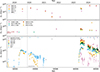 |
Fig. 3. Multiwavelength light curves of AT2019aalc. Bottom plot: X-ray and extinction-corrected and host-subtracted optical/UV. Middle plot: Multifrequency short-baseline radio. Upper plot: Extinction-corrected and host-subtracted IR. Here we show only the positive ZTF fluxes based on the forced photometry results. The dashed gray vertical line indicates the IceCube detection of the high-energy neutrino event IC191119A. The short, purple vertical lines on the top of the bottom panel indicate the peak times of the X-ray flares while the blue ones show the times the main optical r-band flare and later the bumps. The gray ‘S’ letters represent the observing times of the optical spectra. |
Prior to the discovery of AT2019aalc, the host galaxy of the transient was monitored by several optical surveys. To study the pre-discovery optical variability of AT2019aalc, we performed aperture photometry of the All-Sky Automated Survey for Supernovae (ASAS-SN: Shappee et al. 2014; Kochanek et al. 2017) and the Catalina Real-Time Transient Survey (CRTS: Djorgovski et al. 2011). In addition, Palomar Transient Factory (PTF Law et al. 2009) magnitudes were extracted from the PTF Lightcurve Table6. No obvious signs of flaring activity is visible between April 2005 and the discovery of the transient in January 2019 by ZTF (see Fig. 4).
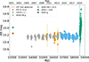 |
Fig. 4. Pre-flare long-term optical light curves of the AGN hosting AT2019aalc starting approximately 14 years before the discovery of the transient in January 2019. The transient is indicated with a blue vertical line. |
The UV monitoring of the source started on 2023-06-23 around 20 days before the optical peak of the second flare. The U-band peak is coincident with the optical peak, while the shorter wavelength bands peaked 2 − 4 weeks later. Furthermore, the U- and UVW2-band peaks occur closer in time than the UVW1 and UVM2 peaks, suggesting a complex SED evolution near the maximum. We note that right after the r-band peak, a short plateau phase started in optical and UV. The transient is most luminous at the shortest wavelength ranges covered by UVOT. The UV emission peaks around Luv ≈ 1044 erg/s in the filter UVW1. After the peak, the UVW2−U color shows reddening. Toward the end of the UVOT monitoring, the measured UVM2 magnitudes decreased back to the level of the baseline GALEX-NUV magnitudes measured between 2007 and 2011.
Comparing the peak UVM2 magnitude of the UVOT monitoring to the GALEX-DR5 (Bianchi et al. 2011) NUV magnitude implies that the UV luminosity increased by a factor of ≈7 with respect to the archival flux. The amplitude of this flare is higher than typically seen for AGN. Only 8 out of the 305 AGN presented in the GALEX Time Domain Survey (Gezari et al. 2013) have larger amplitude NUV variability.
4.2. Infrared
We detected AT2019aalc in all of the three bands observed with the WIRC. The observed magnitudes are plotted in the top panel of Fig. 3. We compare these to pre-flare magnitudes presented in the 2MASS All-Sky Catalog of Point Sources (Cutri et al. 2003). The observed magnitudes in April 2000 are higher with ≈0.5 mag in J-, and Ks-bands and ≈0.6 mag in H-band indicating the clear brightening of the IR counterpart with respect to archival data.
The top panel of Fig. 3 shows the light curve starting just before the first optical flare. The distinct first dust echo flare peaks around six months after the first optical peak. The rise of the dust echo of the second flare also becomes visible in the latest WISE data releases. The light curve varies by around 0.3 mag in W1 and 0.4 mag in W2 before the dust echo flare, which is consistent with statistical AGN variability (Berk et al. 2004). In contrast, the dust echo presents an increase of 1.0 mag in W1 and 1.2 mag in W2 after the first optical flare. Following the second optical flare, the IR light curve shows a brightening of around 1.3 mag in both bands and is increasing when the optical flare is already decaying. Because the brightness is significantly above the limiting magnitude where Eddington bias becomes an issue for stacked single-exposure photometry (Necker et al. 2025), we can estimate the pre-flare mid-IR color using the median of the light curve prior to the dust echo flare with mW1 − mW2 ≈ 0.6. Although there is clear AGN activity prior to the dust echo flare, this is still below the widely used AGN identification cut of mW1 − mW2 ≥ 0.8 (Stern et al. 2012). However, according to the reliability of WISE selection as a function of a simple W1−W2 color selection (Stern et al. 2012), the color of AT2019aalc suggests a reliability of only ≈70%. With the onset of the dust echo, the IR emission becomes dominated by the heated dust. The change from bluer to redder colors comes from cooling of the dust. The re-brightening of the second dust echo is consequently accompanied by another color change toward the blue, shown in Fig. 5.
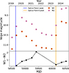 |
Fig. 5. Long-term IR variability of AT2019aalc. The W1−W2 color indicates heated dust as the dominant origin of the IR emission. The second optical flare is accompanied by another IR flaring episode with color change toward the blue. The plotted magnitudes are in the Vega system and have been corrected for extinction but not for host-galaxy contribution, allowing the full evolution between the flares to be visible. |
Notably, AT2019aalc is not part of the Flaires sample (Necker et al. 2025), a list of dust-echo-like infrared flares interpreted as extreme AGN accretion events or TDEs. This is because the broad application of the Flaires pipeline necessarily included a strict cut on extraneous variability that AT2019aalc did not pass. However, the authors did note that a desirable relaxation of this criterion would include AT2019aalc. The source, however, is part of the dust echo sample of van Velzen et al. (2024), and notably it has the highest dust echo flux of all ZTF transients.
4.3. X-ray
The 0.3–10 keV X-ray luminosity evolution is shown in the bottom panel of Fig. 3 while the count rate variability is plotted in the top panel of Fig. 6. The first flaring episode peaked at a luminosity of LX ≈ 6 × 1042 erg s−1 in the end of June 2023 (see Fig. 3.) This flare peaked two weeks before the optical peak. The count rate dropped by a factor of ∼10 within a timescale of ∼60 days. Later, the X-ray emission showed limited variability for several months. A hint of increased emission was detected in mid-February 2024, which was also followed by a bump in the optical and UV light curves around two weeks later. In the end of April 2024, a rapid and extreme flaring episode started in X-rays that lasted less than a month but reached a luminosity of LX ≈ 4 × 1043 erg/s, which is almost a magnitude larger than the peak of the first X-ray flaring episode. Interestingly, this X-ray flare was also accompanied by a bump in the optical 1 − 2 weeks later. A similarly luminous and rapid flare was detected in August 2024 and once more, accompanied by an optical bump 1 − 2 weeks later. Around 90 days passed between the second and third and the third and fourth X-ray peaks.
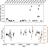 |
Fig. 6. Swift-XRT count rate and photon index variability of AT2019aalc during the observing campaign. In most cases are data is well described by a power-law spectral model (black), except during the two recent flaring episodes, where blackbody or combined models are preferred (red). The blackbody temperature is indicated on the red y-axis. |
In Fig. 7 we show the source spectrum derived from the observing campaign. The spectral index of the stacked spectrum fit with a power-law+blackbody model is  while the blackbody temperature is
  eV. These imply an overall unabsorbed luminosity value of L
 erg/s. The mean count rate of the observations is 0.038 ± 0.001 cts s−1. The photon index variability of AT2019aalc is presented in the bottom panel of Fig. 6.
 |
Fig. 7. Overall Swift-XRT 0.3 − 10 keV spectrum of AT2019aalc. We binned the spectrum to have a minimum of five counts per spectral bin and fit with an absorbed blackbody plus power-law model. |
AT2019aalc (= SRGe J152416.7+045118) was observed by the eROSITA (Sunyaev et al. 2021) soft X-ray telescope four times starting from 2020-02-02 (roughly half a year after the peak of the first optical flare) with a 6 months cadence. The X-ray light curve reached a plateau between August 2020 and January 2021 with a flux of FX ≈ 4.6 × 10⁻¹³ erg cm−2s−1 in the energy range of 0.3 − 2 keV. The source had a soft thermal spectrum described with a blackbody temperature of kT = 172 ± 10 eV (van Velzen et al. 2024). One observation with XMM-Newton Observatory (Jansen et al. 2001) was performed on 2021-02-21 during a period of optical quiescence. The best-fit power-law index and the observed 0.3 − 8 keV flux of this observation were  and F
and F erg cm−2s−1 (68% confidence), respectively (Pasham 2023).
4.4. Radio
4.4.1. Temporal evolution
The pre-flare system was detected in the NRAO VLA Sky Survey (NVSS, White et al. 1997) in February 1995 and in the FIRST survey in February 2000 (both at 1.4 GHz) with peak flux densities of 6.0 ± 0.5 mJy and 6.2 ± 0.1 mJy respectively, suggesting no substantial variability. These flux densities correspond to a monochromatic radio luminosity of ≈2 × 10²² W Hz−1 measured at 1.4 GHz, which is typical for Seyfert galaxies (Meurs & Wilson 1984).
Later, the transient’s sky location was observed in the Karl G. Jansky Very Large Array Sky Survey (VLASS, Lacy et al. 2020). The VLASS observes the entire sky visible to the VLA at 2 − 4 GHz wide band three times. Our source was detected with peak flux density values of 2.9 ± 0.2 mJy/beam (on 2019-03-14), 5.7 ± 0.2 mJy/beam (on 2021-11-06) and 4.0 ± 0.2 mJy/beam (on 2024-07-20), corresponding to 3 GHz radio luminosities (νLν) of 3 × 1038 erg s−1, 5 × 1038 erg s−1 and 3.5 × 1038 erg s−1, respectively. This factor of ≈2 increase in flux from the first VLASS epoch (three months before the first optical peak) to the second VLASS epoch (2 years post-peak) is statistically significant (at the 8σ-level, as estimated from the rms in the VLASS “Quick Look” images, van Velzen et al. 2024).
In addition, we found a radio source at the position of AT2019aalc in the first data release of the Rapid ASKAP Continuum Survey (RACS: McConnell et al. 2020). The source was observed in two different fields and, consequently, at two different epochs. The observed peak flux densities of 9.2 ± 0.5 mJy/beam (on 2019-04-24) and 9.5 ± 0.5 mJy/beam (on 2020-04-30) correspond to a 888 MHz radio luminosity of ≈2.5 × 1038 erg s−1 and indicate that the radio flare observed in the VLASS data started at least 300 days after the peak of the first optical flare, sometime between April 2020 and November 2021.
The radio luminosity in the beginning of our ATCA monitoring was at the same level (5 × 1038 erg s−1) when the source was observed for the second time in the VLASS in April 2021. Since the radio brightness does not show rapid variability during the months of our ATCA monitoring, we can reasonably assume that the sharp increase resulted in a long-lasting plateau. We present the ATCA radio multifrequency light curves of AT2019aalc together with the archival observations in the middle panel of Fig. 3.
4.4.2. The radio spectrum
To further characterize the radio emission of AT2019aalc, we derived the radio spectral index of the radio source in each epoch of our ATCA monitoring. The spectral index between 2.1 GHz and 9.0 GHz (α, defined as S ∝ να) does not show any obvious signs of variability on a timescale of 9 months. We give an average spectral index of  . We calculated a pre-flare spectral index using the VLASS epoch 1 and RACS epoch 1 flux densities. The spectral index we derived this way is
  . Our high-frequency K-band observations centered at 18 GHz, however, do not follow the steep power-law and suggest a turnover between 9 GHz and 18 GHz (see Fig. 8).
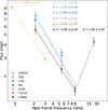 |
Fig. 8. Radio spectra of AT2019aalc spanning 3–18 GHz obtained through our ATCA monitoring. We derived a prior radio flare spectrum between 888 MHz and 3 GHz from archival fluxes. The times in the legend are relative to the peak of the second optical flare. |
4.4.3. VLBI detection
The naturally weighted VLBI map of AT2019aalc is presented in Fig. 9. We detected a single radio-emitting feature with a signal-to-noise ratio of ≈19σ. We obtained the following parameters of the fit component: a total flux density of S = 21 ± 1.8 mJy and a size of d = 2.23 × 1.39 ± 0.3 × 0.3 mas at a position angle of ϕ = −73.3°. We calculated the uncertainties of the flux density and size parameters following the formulas of Fomalont (1999). The minimum resolvable size (θlim) of a Gaussian component fit to naturally weighted VLBI data was calculated following Kovalev et al. (2005). This yields θlim = 1.05 × 0.81 mas, implying that the fit Gaussian component is resolved.
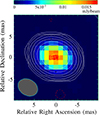 |
Fig. 9. Naturally weighted 1.7 GHz EVN+e-MERLIN high-resolution VLBI map of AT2019aalc. The peak brightness is 17.3 mJy beam−1. The gray ellipse in the lower-left corner represents the Gaussian restoring beam. Its parameters are 4.82 mas × 3.7 mas (FWHM) at a major axis position angle of PA |

We calculated the brightness temperature of the radio-emitting feature found at the position of AT2019aalc using the following equation (Condon et al. 1982; Ulvestad et al. 2005):
 (1)
(1)
where S is the flux density of the fit Gaussian component measured in Jy, θmaj and θmin are the major and minor axes full width at half maximum (FWHM) of the fit component in mas, and ν is the observing frequency in GHz. The obtained brightness temperature is Tb = (3.0 ± 0.8)×108 K at 1.7 GHz. The brightness temperature is an effective parameter that is commonly used in radio astronomy to describe the physical properties of emitting material in astrophysical objects (e.g., Lobanov 2015).
4.5. Spectroscopic results
We present the archival and the newly obtained optical spectra of AT2019aalc in Fig. A.1, marking the notable emission lines. In the following, we highlight the remarkable line detection of the pre-flare spectrum observed before the first optical flare, the one observed between the two flares (post-flare-1 spectrum) and the five spectra taken during the second flare (over-flare-2 spectra).
4.5.1. Pre-flare spectrum
A spectrum of the pre-flare system was observed in April 2008 by the SDSS spectrograph. We present this spectrum with the best fits for the stellar and gas components in Fig. A.2. We identified strong Balmer emission lines. We calculated FWHM(Balmer) ≈ 2800 km s−1 for the broad component of the Balmer lines in the pre-flare spectrum, which is typical for an unobscured, broad-line AGN. The line widths (FWHM(Balmer) ≈ 2600 km s−1) presented in the SDSS DR7 broad-line AGN catalog (Liu et al. 2019) for our source are consistent with this classification.
Several forbidden lines such as [O III] λ4959 and [O III] λ5007, [S II] λ6716, [S II] λ6731, and [N II] λ6584 were detected. These lines are produced in the narrow-line region (NLR) in AGN. We detected the [O II] λ3726+ [O II] λ3729 line doublet, which is a potential indicator of AGN-driven outflows (e.g., Santoro et al. 2020). The pre-flare spectrum also indicates the detections of two high-ionization coronal lines ([Fe X]λ6375 and [Fe XIV]λ5303) which are further discussed below.
4.5.2. Post-flare-1 spectrum
The first LRIS spectrum was observed almost two years after the first optical flare and two years before the second one. In this spectrum, prominent Balmer lines were detected, similar to the SDSS spectrum. The spectrum exhibits the aforementioned forbidden lines detected in the archival spectrum. We also identified the BF lines O IIIλ3133 and He IIλ3203.
The high ionization coronal lines [Fe VII]λ6087, [Fe X]λ6375, [Fe XIV]λ5303, and [Fe vii]λ5721 were detected. Furthermore, we identify the [Ne V] emission lines at 3345 Å and 3426 Å in the spectrum. Note that the pre-flare SDSS spectrum does not cover these wavelengths, and therefore these lines are not necessarily related to the optical flares discussed here. These neon lines are prominent emission lines originating from the inner NLR excited by the AGN via photoionization or shocks, and are sometimes considered as coronal lines (e.g., Cann et al. 2020).
4.5.3. Over-flare-2 spectra
We performed five optical spectroscopic observations of AT2019aalc during the second flare. These are characterized by a blue continuum with several more emission lines than the spectra discussed above. We compared the second LRIS spectrum of AT2019aalc (covering the broadest wavelength range) with a composite SDSS spectrum based on 10112 Seyfert 1 galaxies published in Pol & Wadadekar (2017), in Fig. 10. This comparison shows similarities but also remarkable differences discussed below.
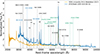 |
Fig. 10. Over-flare-2 LRIS spectrum of AT2019aalc in comparison with the SDSS composite spectrum of 10112 Seyfert 1 galaxies published in Pol & Wadadekar (2017) and normalized between 7400 and 7500 Å. The most remarkable lines are shown with vertical lines. The most notable differences are the appearance of the Bowen lines (marked with blue) and the high-ionization coronal lines (marked with green) in the spectrum of AT2019aalc. |
Over the second optical flare, strong Balmer lines were detected, with two of them (Hδ and Hη) appearing only in the over-flare-2 spectra. We identified the BF line complex N IIIλ4640+He IIλ4686. The complex was not detected in the earlier spectra. The relative strength of the BF complex to Hβ reached a maximum on 2023-07-11, very close to the optical continuum peak (2023-07-13). As we detected the Bowen line N IIIλ4640 even 315 days after the optical peak of the second flare, we conclude that it persists over long timescales. We also find hints of O IIIλ3760, which is also known as a Bowen line (Selvelli et al. 2007). However, due to a possible blending from Fe VIIλ3759, its detection is questionable. Nevertheless, this Bowen line is created through the same channel (O1) as the above-discussed O IIIλ3133, which supports the hint of detection. O IIIλ3760 was detected in some metal-rich TDEs before (Leloudas et al. 2019), such as AT2019dsg (Cannizzaro et al. 2021).
We detected the high-ionization coronal lines identified in the post-flare-1 LRIS spectrum over the second flare in each spectrum. Furthermore, a new coronal line appears: [Fe XI] λ7892, which has an ionization potential of 262 eV (e.g., Reefe et al. 2022). We also detected the [Ne V] emission lines at 3345 Å and 3426 Å in the second LRIS spectrum, as well as in the post-flare-1 spectrum.
5. Discussion
5.1. Spectroscopic properties
5.1.1. Balmer lines
AT2019aalc exhibits prominent Balmer lines in each spectrum. In addition, a more complex structure of these lines appears in the late-time over-flare-2 spectrum. The Balmer series lines here exhibit a redward wing. In some cases, however, it might result from blending with other lines, such as Hδ and the BF line N iii λ4103. Interestingly, the post-flare-I spectrum shows a similar structure to the Balmer line series.
5.1.2. Bowen fluorescence lines
Wavelength coincidences between emission lines (“line fluorescence”) can be an important source of radiative excitation. The BF mechanism in astrophysical environments is a good indicator of absorbed EUV−soft X-ray flux (at wavelengths shorter than the He II Lyman limit of hν ≥ 54.4 eV), as these high-energy photons are converted into the He II Lymanαλ 303.782 Å emission required for the excitation of the O III and N III lines in the optical and NUV regimes (Netzer et al. 1985; Netzer 1990). This is consistent with the multiple soft X-ray flares and the extreme UV luminosities of AT2019aalc. The BF line O IIIλ3133 has been observed in the BFFs AT2017bgt (Trakhtenbrot et al. 2019) and AT2021loi and only in a few Seyfert galaxies before (e.g., Malkan 1986; Schachter et al. 1990). However, we note that due to the atmospheric cutoff at ≈ 3100 Å these lines are difficult to detect. This line is typically weaker in regular Seyfert galaxies than in the case of AT2019aalc (see Fig. 10). The BF line N IIIλ4640 is not generally seen in AGN (e.g., Vanden Berk et al. 2001). However, it has been observed in several optical TDEs (Charalampopoulos et al. 2022) and BFFs (Trakhtenbrot et al. 2019; Makrygianni et al. 2023).
The detection of a BF line almost two years after the first optical flare of AT2019aalc suggests its long persistence, similar to the BFFs studied by Trakhtenbrot et al. (2019). In the case of AT2017bgt, this line was still detected 470 days after the discovery of the transient. The Bowen features in F01004-2237 were detected even ≈8 years after the initial flare (Tadhunter et al. 2021). We compare the over-flare-2 high-resolution LRIS spectrum of AT2019aalc to the spectra of BFFs, a TDE-Bowen, and a repeating partial TDE in Fig. 11 around the N IIIλ4640+He IIλ4686 complex. We also compare the second LRIS spectrum of AT2019aalc with the LRIS spectrum of AT2021loi in Fig. 12, zooming into the O IIIλ3133+He IIλ3203 region.
 |
Fig. 11. Second LRIS spectrum of AT2019aalc zoomed in on the He IIλ4686+N IIIλ4640 complex region and compared to those of the BFFs AT2021loi (Makrygianni et al. 2023) and AT2017bgt (Trakhtenbrot et al. 2019), the peculiar transient event AT2019avd (Trakhtenbrot et al. 2020), the repeating TDE AT2020vdq (Somalwar et al. 2025b), and the TDE-Bowen AT2018dyb (Pan et al. 2018). All of the plotted spectra were normalized at 5200 Å. |
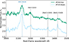 |
Fig. 12. Second LRIS spectrum of AT2019aalc zoomed in on the O IIIλ3133+He IIλ3203 complex region and compared to that of the BFF AT2021loi published by Makrygianni et al. (2023). The spectra were normalized at 5200 Å. |
The He ii λ4686 emission line is commonly detected in AGN and known as a recombination line, tracing ionized gas in the vicinity of the central SMBH responsible for the photoionization (e.g., Wang & Kron 2020). This line is known to be created by photoionization due to (soft) X-ray photons with a rough correspondence of 1 He II photon emitted for each 0.3 − 10 keV X-ray photon (Pakull & Angebault 1986; Schaerer et al. 2019; Cannizzaro et al. 2021). In the spectra of AT2019aalc, He IIλ4686 is detected together with strong N III and O III BF lines and He IIλ3203, indicating its relation to the BF mechanism. Furthermore, we calculated a maximum line intensity ratio of F(He II)/F(Hβ) ≈ 0.7, which significantly exceeds the typical ratios estimated for AGN (earlier Vanden Berk et al. (2001) estimated ratios of F(He II)/F(Hβ) ≤ 0.05 while Shirazi & Brinchmann (2012) gives F(He II)/F(Hβ) ≤ 0.1). Our value, however, is more comparable with the line ratio estimated for the BFF AT2017bgt (F(He II)/F(Hβ) ≈ 0.5, Trakhtenbrot et al. 2019).
5.1.3. Coronal lines
Based on a study of SDSS spectra, Wang et al. (2012) reported the discovery of seven extreme coronal line emitter (ECLE) galaxies, which show extremely strong coronal lines. Numerous TDEs were also found to exhibit coronal lines. The BFF AT2021loi (Makrygianni et al. 2023) and the spectacular transient event AT2019avd (Malyali et al. 2021) also exhibit strong coronal lines. The BFF F01004-2237 showed variable coronal lines on a timescale of 3 years (Tadhunter et al. 2021). Based on the publicly available spectra of AT2017bgt on the Transient Name Server7 (TNS) we detect enhanced coronal line emission in this BFF, too.
The most plausible origin of the ECLEs is that they represent echoes of a past TDE outburst (Wang et al. 2012; Hinkle et al. 2024b; Koljonen et al. 2024; Newsome et al. 2024). Notably, Short et al. (2023) revealed that the TDE AT2019qiz more likely follows the line ratio correlations of ECLEs instead of regular AGN. The coronal lines in AT2019qiz appeared around 400 days after the optical peak, further supporting this scenario. Moreover, the estimated rate of coronal line emitters is consistent with the estimated rate of TDEs (Wang et al. 2012). Later, Callow et al. (2024) discovered 9 new ECLEs using SDSS spectra and refined the previous rate calculations. They found that the ECLE rates are below the TDE rates; however, the rates can still be consistent with the assumption that only 10% to 40% of all TDEs produce variable coronal lines. According to Wang et al. (2012), the origin of the coronal lines in ECLEs can be explained with the liberation of Fe from dust grains that were destroyed by the echo of past TDE flares. A follow-up spectroscopic analysis of the original ECLE sample of Wang et al. (2012) revealed that the coronal line signatures did not recur in five out of the seven objects, supporting their transient light echo origin (Clark et al. 2024). The large dust echo of AT2019aalc is consistent with this picture. Furthermore, the TDEs with coronal line detection have more luminous IR dust echoes compared to other optical TDEs. AT2019qiz is one of the few TDEs included in the accretion flare sample of van Velzen et al. (2024), due to its strong dust echo. Another coronal line-detected TDE AT2017gge is part of the mid-infrared (MIR) dust echo flare sample of Hinkle (2024), which contains 19 ANTs with high dust covering factors. The extreme dust echo seems to characterize the BFFs as well. The BFFs AT2021loi, AT2017bgt, OGLE17aaj and the candidate BFF AT2019avd are present in the above-mentioned MIR dust echo sample (Hinkle 2024) and two of them are also part of the Flaires sample of dust-echo-like IR flares (Necker et al. 2025). The BFF F01004-2237 exhibited a MIR flare (Dou et al. 2017). The Bowen line transient AT2019pev shows strong high-ionization coronal lines (Frederick et al. 2021; Yu et al. 2022) and is also part of the MIR flare sample of Hinkle (2024). These findings suggest a connection not only between the ECLEs and TDEs, but also the BFFs.
Figure 13 shows the [Fe X]λ6375 versus the [O III]λ5007 luminosities of the ECLEs, the coronal-line detected TDEs and BFFs and AT2019aalc, together with the coronal-line detected SDSS Seyfert sample of Gelbord et al. (2009). For this plot, we performed modeling of the publicly available spectra8 of several TDEs and BFFs using PYQSOFIT, following the procedure described in Sect. 3.5. These are the TDEs: AT2017gge (2017-09-14, EFOSC2); AT2018dyk (2018-08-08, LRIS); AT2018bcb (2018-05-06, EFOSC2); AT2021qth (2022-05-26, LRIS); AT2022upj (2022-10-26, DBSP); and the BFFs: AT2017bgt (2017-02-23, LRIS) and F01004-2237 (2018-08-13, EFOSC2). Absolute fluxes, and hence derived luminosities, are subject to systematic uncertainties from slit losses and atmospheric extinction differences. We adopt a conservative ±20% uncertainty on the flux scale to account for these effects, which is combined in quadrature with the statistical uncertainties from the PYQSOFIT spectral fits. This method is applied only to cases where the slit position angle differed at least five degrees from the parallactic angle. Fig. 13 clearly implies an offset of the ECLEs, BFFs and AT2019aalc from the regular AGN sample. We note that the only object in the sample of Gelbord et al. (2009) classified as a galaxy rather than an AGN is, in fact, the same source as one of the variable ECLEs (which appear as nearly overlapping points in our plot). No publicly available spectra were found of the TDEs AT2021dms, AT2024mvz and AT2021acak while in the case of AT2017gge, it was not possible to safely distinguish [Fe X]λ6375 from Hα. We note that AT2021acak exhibited two distinct optical flares (Li et al. 2023), with the second being more luminous, and showed a He IIλ4686+N IIIλ4640 complex similar to that of AT2019aalc.
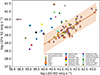 |
Fig. 13. [Fe X]λ6375 versus [O III]λ5007 luminosities for (a) ECLEs (Wang et al. 2012; b) variable ECLEs (Yang et al. 2013; c) AT2019aalc (this work); (d) the TDEs AT2019qiz (Short et al. 2023), AT2018dyk, AT2022fpx (Lin et al. 2025), AT2018bcb, AT2021qth and the TDE/QPE AT2022upj; (e) the repeating pTDEs AT2020vdq (Somalwar et al. 2025a) and ASASSN-14ko; (f) the BFFs AT2017bgt, AT2021loi (Makrygianni et al. 2023), F01004-2237; and (g) the BFF candidate AT2019avd (Malyali et al. 2021). A sample of different types of Seyfert galaxies (Gelbord et al. 2009) is plotted as well. The orange line represents a linear fit to the sample, and the orange shaded area represents the 95% prediction interval. The transient sources have clearly higher [Fe X]/[O III] luminosity ratios than the Seyfert sample. |
5.2. Optical re-brightening
The long-term ZTF light curve of AT2019aalc shows two well-separated flares. Both flares rose quickly and reached their peaks within two months, followed by a slow decay on yearly timescales. Generally, TDEs are characterized by smoothly and rapidly declining light curves (F ∝ t−5/3) as expected from mass fallback considerations (Rees 1988), and without any prominent bumps in the case of full disruption. AT2019aalc in turn has a slowly decaying first flare with a power-law fit returning a power-law index of b ≈ −0.45 and a second flare that began 4 years after the initial flare. The first systematically identified repeating partial TDE (AT2020vdq), however, shows not just a double-peaked long-term optical light curve, but its second flare is ≈3 times more luminous compared to the first one (Somalwar et al. 2025b). This implies an even more significant optical re-brightening than the one detected in AT2019aalc. In contrast, the candidate pTDE AT2022dbl exhibits with a brighter first flare. The second flare of partial TDEs is expected to follow a steep declining with a power-law of t−9/4. In the case of AT2020vdq and AT2022dbl, the second flares declined slower than this (Somalwar et al. 2025b; Makrygianni et al. 2025), but still faster than the second flare of AT2019aalc, which declined with a power-law index of b ≈ −0.23. Notably, AT2020vdq and AT2022dbl both exhibit slower-declining second flares compared to their first flares, similar to AT2019aalc.
Interestingly, most of the sources of the small sample of classified BFFs show optical re-brightening or bumps. Fig. 14 shows the optical evolution of the three BFFs with detected re-brightening episodes, together with AT2019aalc. The optical light curve of AT2017bgt shows a bump roughly 400 days after its initial flare which is also clearly visible in the binned light curve published in Trakhtenbrot et al. (2019). Originally, F01004-2237 had undergone a luminous flare (Tadhunter et al. 2021) in 2010, and later Trakhtenbrot et al. (2019) classified it as a BFF. The binned light curve of F01004-2237 published in Makrygianni et al. (2023) shows a bump around a year after its peak. We investigated the recent activity of this source and found that it significantly re-brightened in 2021 based on its ATLAS monitoring. The recent flare was more luminous than the first one and declined faster. In addition to these two BFFs, AT2021loi shows a bump when declining, roughly a year after the first flare reached its peak. Makrygianni et al. (2023) suggests that optical re-brightening or bumps seen when decaying might be common features of BFFs. OGLE17aaj, has not shown a clear optical re-brightening. However, a bump likely appears roughly a year after the peak, similar to AT2017bgt and AT2021loi. The BFFs classified so far tend to have remarkable variances in their optical light curve evolution despite the similarities. These might be explained by different subclasses of BFFs, similarly to regular TDEs, where different subclasses were defined based on their light curve evolution (e.g., Charalampopoulos et al. 2023).
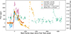 |
Fig. 14. Long-term optical light curves of AT2019aalc and three classified BFFs. The light curves indicate that optical re-brightening and bumps may be a common property of BFFs. However, the various sources differ in when these episodes start with regard to the initial flares. |
5.3. Radio characteristics
5.3.1. Possible explanations of the long-term radio flare
In this subsection we discuss the long-term radio variability of AT2019aalc. The radio source experienced a brightening of its flux density by a factor of two on a timescale of less than 1.5 years, followed by a long-term plateau (≥3 years) indicated by the archival radio survey data and our ATCA monitoring. Although radio variability on yearly timescales is a common phenomenon of Seyfert galaxies, the sharp, high-amplitude radio flare and especially the long-term plateau are generally not seen in intrinsically variable Seyfert galaxies (e.g., Mundell et al. 2009; Koay et al. 2016) and therefore require further investigation. The unusual radio spectrum with a high frequency turnover is also discussed below.
-
The brightness temperature of Tb = (3.0 ± 0.8)×108 K at 1.7 GHz significantly exceeds 105 K, known as an upper limit for supernova remnants and He II regions in star-forming galaxies (Condon 1992). Consequently, the radio emission we detected must be non-thermal and originate from physical processes associated to AGN-like (including TDEs) activity (see Bontempi et al. 2012 as an example of how the estimated brightness temperatures help characterize the radio emission of Seyfert galaxies). This way, we can also safely rule out thermal free-free emission from the accretion disk or the dusty torus (e.g., the case of NGC 1068, Gallimore et al. 1997) as the origin of the detected radio emission.
-
Advection-dominated accretion flows have also been proposed to explain the origin of the radio emission of low-luminosity AGN (e.g., Seyfert galaxies, Mahadevan 1997). Assuming that accretion flows dominate the radio emission of AT2019aalc, following Yi & Boughn (1998) we estimate an expected 5 GHz radio luminosity of L5 GHz ≈ 4 × 1035 erg s−1, 3 orders of magnitude lower than the observed one, clearly indicating that these cannot explain the observed radio emission.
-
Magnetized coronal winds originating from the AGN accretion disk could produce the non-thermal radio emission of AT2019aalc. Laor & Behar (2008) found a correlation of log(LR/LX)≈ − 5 studying the Palomar–Green (PG: Green et al. 1986) radio-quiet quasar sample (in good agreement with the correlation found for coronally active stars by Guedel & Benz (1993)). Later, Behar et al. (2015) came to the same conclusion using a sample of seven radio-quiet Seyfert galaxies. For our source, based on the mean ATCA C-band and the extrapolated Swift/XRT 2 − 20 keV luminosities, we estimate a ratio of log(LR/LX)≈ − 2, suggesting that magnetized coronal winds alone cannot fully explain the observed radio emission of AT2019aalc. Moreover, coronal emission should be highly variable at radio wavelengths.
-
Out-flowing synchrotron-emitting material induced by enhanced accretion is commonly detected in AGN and TDEs in the forms of non-relativistic outflows or relativistic jets (e.g., Paragi et al. 2017; Mohan et al. 2022; Kozák et al. 2024). The high brightness temperature of the EVN-detected radio feature indicates its radio core identification. The steep (α ≪ −0.5) radio spectrum indicates the presence of another, steep-spectrum synchrotron-emitting component(s) in the system, as radio cores are characterized by a flat radio spectrum. The spectrum may be the composition of the flat-spectrum radio core and the additional, steep-spectrum component(s). The high-frequency turnover around 9 GHz supports the idea of a newly ejected radio-emitting component.
5.3.2. The radio spectrum
The turnover suggests the multicomponent nature of the spectrum. Radio spectra with high-frequency excesses have been observed in a few radio-quiet narrow-line Seyfert 1 galaxies (Berton et al. 2020). These sources are thought to be kinematically young AGN with small linear sizes or heavily absorbed AGN. The high-frequency peak might be explained with the kinematic age of a newly ejected component. These extremely young radio sources therefore peak at very high frequencies (e.g., Berton et al. 2020). The low-frequency peak is more likely originating from star formation activity instead of AGN emission, since the latter is absorbed at these frequencies due to synchrotron self-absorption (SSA) or free-free absorption (FFA).
However, in the case of AT2019aalc, the large-amplitude variability concluded from the VLASS observations and the EVN detection of a high brightness temperature (Tb ≫ 105 K) feature at 1.7 GHz clearly imply AGN-like activity over a star formation scenario at lower frequencies. Therefore, our results indicate that the radio spectrum of AT2019aalc is strongly dominated by AGN activity below 10 GHz as well, even if a contribution from star formation, especially at 2.1 GHz, is probable.
A newly ejected component can explain the high-frequency excess, whilst the low-frequency part originates from optically thin synchrotron emission of the AGN. Thus, the overall spectrum represents a superposition of past and recent AGN activity, indicative of its recently enhanced, intermittent behavior. Järvelä et al. (2021) states that restarted AGN activity can explain at least some of the radio spectra studied by Berton et al. (2020). Intermittent activity is further supported by theoretical models highlighting that sources with high accretion rates are more prone to this kind of behavior (Czerny et al. 2009).
5.4. X-ray properties
The X-ray spectra of AGN at energies above 2 keV have a power-law-like shape. These X-ray photons are believed to be triggered by Compton up-scattering of the accretion disk photons off hot electrons surrounding the disk, in a hot (≈109 K) optically thin corona above the disk (e.g., Kammoun et al. 2015). Below 2 keV some AGN show an excess in their spectrum referred to as the soft X-ray excess. It can be modeled well by a blackbody model with a best-fit temperature in the range 0.1 − 0.2 keV. The origin of the excess might be explained via Comptonized disk emission. The reflection of hard X-ray photons from the surface of the disk can also account for the excess (Done et al. 2012).
The X-ray spectrum of AT2019aalc exhibits a non-thermal component with a power-law index of Γ ≈ 3.3 and an unusually soft thermal component with a blackbody temperature of kT ≈ 95 eV. Most of the BLSy1s typically have a harder X-ray spectrum with a power-law index of Γ = 1.7 − 2 (e.g., Pons & Watson 2014). AT2019aalc exhibits properties that are more common in sources characterized by enhanced accretion, e.g., NLSy1s or TDEs which both have typically soft X-ray spectra with Γ > 2 (Boller et al. 1996; Saxton et al. 2020).
The soft X-ray flux of Seyfert galaxies was found to be correlated well with the observed fluxes in the coronal line [Fe X] λ6375. The coronal lines to X-ray flux ratio is log(f[Fex]/fx) = − 3.43 ± 0.55 for both broad and narrow-line Seyfert 1 galaxies (Gelbord et al. 2009). For AT2019aalc we estimate values of log(f[Fex]/fx)≈ − 3.45 when optical spectroscopic and X-ray observations were performed nearly simultaneously (due to the rapid X-ray variability, we consider only observations taken on the same day). This suggests that this coronal line is excited by the X-ray flares discussed here instead of past X-ray flares that are thought to power the ECLEs.
The reoccurring optical/UV bumps appearing during the decay of the main optical flares are likely driven by the soft X-ray flares, which lead these outbursts only by a couple of weeks. The soft X-ray excess appears to be more dominant during these flares. Interestingly, the soft X-ray flares show hints of quasi-periodicity of ≈90 days. A few Repeating Nuclear Transients (RNTs) were discovered in the past few years: Quasi-Periodic Eruptions (QPEs) exhibit soft X-ray flares on time-scales of hours to days, while partial TDEs exhibit such flares on timescales of months to years (e.g., Chakraborty et al. 2021; Quintin et al. 2023; Miniutti et al. 2023; Nicholl et al. 2024). We note that another BFF, AT2020afhd, shows hints of quasi-periodic soft X-ray flares according to its Swift/XRT monitoring. This source is included in the Living Swift XRT Point Source Catalogue (LSXPS: Evans et al. 2023) as LSXPS J031335.6−020905. The potential connection between BFFs and QPEs should be explored in future studies.
5.5. SED fitting
Following Reusch et al. (2022), we fit two blackbody models in order to describe the SED of the transient using LMFIT. These curves fit to the optical/UV (blue blackbody) and IR datapoints (red blackbody) are shown in Fig. 15, together with a combined double blackbody fit. The red blackbody fit was introduced in order to account for the IR dust echo. These curves fit the SED around the optical peak of the investigated flare.
 |
Fig. 15. Extinction-corrected and host-subtracted SED of the second flare of AT2019aalc as measured around the optical peak. Two blackbody models to the optical/UV (solid curve) and IR data points (dotted curve) were fit separately. A combined fit (black dashed curve) is also shown. |
The continuum emission of TDEs is described well by a thermal blackbody model (Gezari 2021). The case of AT2019aalc appears to be more complex. The UV emission has a contribution from the BF mechanism and possibly also from Comptonization, explaining the poor fit toward the blue. The excess seen in the WISE bands is possibly due to the non-simultaneous observation with respect to the optical/UV and WIRC observations, as the IR light curve is peaked well after the optical one. The excess in the r-band possibly has a contribution from the early appearance of some Fe lines in this range, but such a significant excess cannot be fully explained with the coronal lines only. Instead, a variable Hα component, given its much larger equivalent width, or reprocessing, is more likely to significantly contribute to the observed excess and warrants consideration.
The inferred blackbody temperature and radius values estimated for the blue blackbody fit are Tblue ≈ 14 000 K and Rblue ≈ 1.5 × 1014 cm, respectively. The blackbody temperature is in the lower range of what is found for optically selected TDEs. However, this value is an order of magnitude lower than the typically estimated in X-ray detected TDEs studied by van Velzen et al. (2020) and Thomsen et al. (2022). On the other hand, the radius is smaller than those calculated for optically selected TDEs, but it is more consistent with the X-ray detected ones. The red blackbody fit resulted in Tred ≈ 1400 K and Rred ≈ 2.8 × 1016 cm.
5.6. The nature of AT2019aalc
AT2019aalc shares similarities with TDEs including the soft X-ray spectrum, the dust echo and the optical flare(s) rising with constant color. The UV bright nature of the transient with a blue optical/UV peak color of NUV−r ≈ 0.2 is another TDE-like feature and not typical for AGN and SNe (Gezari 2021). Bowen lines appear in the spectra of several TDEs even if these are typically weaker than in our case. The most remarkable difference, however, is the fading of the optical emission, which is slower than for any TDE identified so far. The reddening in color when the main optical flares are declining is also atypical for TDEs. However, in a more complex AGN environment, compared to the simpler case of standard TDEs in quiescent galaxies, reprocessing may already be significant at early times, implying that the observed reddening does not necessarily reflect genuine cooling.
The unobscured AGN-like optical spectra, the presence of persistent and strong Bowen lines (O IIIλ3133 and N IIIλ4640), the extremely luminous UV flare, optical emission decaying on yearly timescales, and the optical re-brightening altogether suggest a BFF classification of AT2019aalc. Furthermore, we classify AT2019aalc as an ECLE because of the detection of several strong high-ionization coronal lines.
The mechanism that powers the BFFs is still unclear. TDEs in AGN might play a role. In a single star case, the slowly decaying optical/UV emission might be explained by the dissipation of energy due to the continuous interaction between the stellar debris stream and the pre-existing accretion disk (similarly to the case of the TDE-AGN PS16dtm, Blanchard et al. 2017, and ASASSN-14ko, Huang et al. 2023) or the AGN’s radiation field. According to TDE-AGN simulations, stellar passages can induce substantial perturbations in the inner disk and leave it in a very perturbed state even for years (Chan et al. 2019). The debris-disk interaction results in enhanced accretion and multiple shocks (Chan et al. 2019), notably leading to X-ray emission (Ryu et al. 2024). Consistently within this picture, the soft X-ray flares of AT2019aalc suggest that the emission is linked to the accretion disk. These X-ray flares lead the optical/UV bumps by 1 − 2 weeks, which are detected during the decay of the main flare. The soft X-ray emission is likely reprocessed to optical/UV by the dense environment, explaining the optical/UV flares and the emergence of the BF and coronal lines. The TDE-AGN scenario provides an explanation for one slowly decaying flare with recurring outbursts. However, AT2019aalc exhibits two distinct optical flares. TDE-AGN simulations also revealed that in a case of an initially partial disruption, a surviving core would generate similar heating of the inner disk to the first pericenter passage (Chan et al. 2019; Ryu et al. 2024). Notably, the second flare of AT2019aalc is more luminous than the first one, similarly to the cases of the partial TDE AT2020vdq (Somalwar et al. 2025b) and the BFF F01004-2237. Numerical simulations demonstrated that the even more luminous second flare of a partial TDE might be explained in the following way: tidal energy injection leads to oscillations in the remnant star, and if the thermal energy cannot dissipate within one orbital period, the star expands, making it more susceptible to further tidal disruption and potentially resulting in brighter flares (Liu et al. 2025; Zhong 2025). Liu et al. (2025) claimed that these considerations provide a plausible explanation for the brighter second flare of the partial TDE AT2020vdq. A partial TDE scenario might explain the second optical flare of the other two BFFs (AT2021loi and F01004-223) with double-peaked optical flares as well.
A TDE-in-AGN scenario would explain the TDE-like properties of these sources. The most remarkable differences, such as the slowly decaying optical emission and the continuum emission not being well described by blackbody models, may arise due to the more complex environment in which the TDE occurs, compared to the simpler conditions in quiescent galaxies (“TDEs in vacuum”). TDE-AGN simulations showed that the emergent spectrum of such a system may not be purely thermal as in regular TDEs (Chan et al. 2019). Furthermore, a possible connection between the high-ionization coronal lines (which are most probably related to TDE activity, Wang et al. 2012) and the BFFs (see Fig. 13) is consistent with this picture. A known candidate partial TDE in an AGN is the case of the active galaxy IC 3599. This low-luminosity AGN exhibits periodic soft X-ray flares interpreted as being due to interaction with a partially disrupted star, which results in reoccurring outbursts after each passage of the surviving core around the central black hole (Campana et al. 2015). Notably, IC 3599 has more prominent high-ionization coronal lines than most AGN (similarly to the coronal-line detected transients, see Fig. 13). In addition, IC 3599 is the only known AGN with fading coronal lines (Frederick et al. 2019) a behavior also observed in the TDE AT2019qiz (Short et al. 2023), the BFF F01004-2237 (Tadhunter et al. 2021) and most of the ECLEs (Yang et al. 2013). Another feature AT2019aalc shares with other candidate pTDEs is the HeIIλ4686 + NIIIλ4640 complex, observed in the optical spectra of all five optically selected pTDE candidates (see Fig. 13. in Hinkle et al. (2024a)).
Interestingly, other BFFs also showed weaker pre-transient AGN activity than persistently accreting AGN (Trakhtenbrot et al. 2019; Makrygianni et al. 2023). It suggests that TDEs might have reactivated these AGN. However, between the two main optical flares, AT2019aalc exhibited negative fluxes, i.e., it was fainter than the baseline (see Fig. 2). This behavior suggests a retrograde orbit of the disrupted star relative to the accretion disk, as such encounters gain angular momentum and lead to a subsequent lower AGN state (McKernan et al. 2022). In contrast, a prograde orbit adds angular momentum to the disk, resulting in a higher AGN state, which may explain the light curve of OGLE17aaj, where the source persisted in a high and stable state for years after the peak (Gromadzki et al. 2019), unlike AT2019aalc.
5.7. Radio properties of BFFs
As we studied AT2019aalc in radio in detail, we compare the radio properties with that of the BFFs. Based on the radio observations explained in Makrygianni et al. (2023), AT2021loi has an inverted radio spectrum between 5 and 10 GHz while the source was not detected at 3 GHz. Although no radio spectrum is available for AT2017bgt, we investigated the VLASS QL Images of this BFF to study its radio flux variability. We found a radio source at the optical position of AT2017bgt with flux densities of 3.6 mJy (on 2019-05-21), 6.6 mJy (on 2021-10-19) and 4.5 mJy (on 2024-06-11) at a central frequency of 3 GHz. The pre-flare system was detected in the FIRST (at 1.4 GHz) in July 1998 with a flux density of 0.9 mJy. F01004-2237 was detected with VLBI at 8.4 Ghz; however, it remained undetected at 2.3 GHz, which indicates an inverted spectrum (Hayashi et al. 2024). The BFF AT2020afhd was detected with the VLA at 15 GHz with 0.25 mJy (Christy et al. 2024). If BFFs are explainable with TDE-AGN, the synchrotron emission is likely originating from outflow activity due to the enhanced accretion or, alternatively, from interaction between the unbound debris and the surrounding gas predicted by TDE-AGN simulations (Chan et al. 2019). Radio observations of any newly discovered BFF will be essential to better understand these transients.
5.8. BFFs and high-energy neutrinos
AT2019aalc was associated with the high-energy neutrino event IC191119A (most probable neutrino energy: 177 TeV) detected by the IceCube Observatory (IceCube Collaboration 2019; van Velzen et al. 2024). Motivated by the classification of AT2019aalc suggested by its multiwavelength properties (Sect. 5.6), we searched for spatial coincidences between the earlier-classified BFFs and the neutrino alerts from the IceCube Event Catalog of Alert Tracks (ICECAT-1: Abbasi et al. 2023). We found that the BFF AT2021loi is located within the 90% rectangular uncertainty contour of the high-energy neutrino event IC230511 (most probable neutrino energy: 167 TeV) detected in May 2023 (IceCube Collaboration 2023). In the full likelihood contours published in ICECAT-1, the source is just outside the 90% contour. We present the source positions together with the neutrino best-fit positions and both contours in Fig 16. We also report a coincidence between the prototype BFF AT2017bgt and the high-energy neutrino event IC-200410A. This event, however, is a poorly reconstructed cascade event, and therefore we do not discuss it further here.
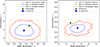 |
Fig. 16. Positional coincidences between high-energy neutrino events and the BFFs AT2019aalc and AT2021loi. The blue and red contours represent the 50% and 90%CL containment detailed contours of the high-energy neutrino events IC191119A (left) and IC230511 (right), respectively. The orange box is the 90%CL rectangular containment region. The neutrino best-fit position is shown with a blue point. The optical positions of AT2019aalc (left) and AT2021loi (right) are marked with green star signs. |
The neutrino associated with AT2021loi was detected 680 days and 290 days after the first and second optical peaks, respectively. Notably, all three nuclear transients (including AT2019aalc) associated with neutrinos exhibited a similar pattern, with neutrino detection occurring 150 − 290 days after the optical peaks. This might be explained with delayed outflow activity (van Velzen et al. 2024). In the case of AT2021loi, the inverted radio spectrum (Makrygianni et al. 2023) is compatible with a newly ejected outflow component, similarly to the case of AT2019aalc. Interactions between the out-flowing material and clouds in the surrounding of the SMBH (Wu et al. 2022) or between ultra-high-energy protons (accelerated in a jet or outflow) and infrared photons from the dust echo (Winter & Lunardini 2023) were proposed to explain the observed neutrino emission of the three nuclear transients. These findings indicate that outflows play an important role in the neutrino production. A case study for AT2021loi would help further constrain the neutrino production models of nuclear transient sources.
If the connection between the high-ionization coronal line detection and the unusually large dust echos of nuclear transients is real, this can be used to reveal more sources with strong dust echoes and therefore more candidate neutrino sources. Notably, both AT2019aalc and AT2021loi are characterized by significant dust echoes (van Velzen et al. 2024; Hinkle 2024: see also Sect. 4.2) and unusually strong high-ionization coronal lines (Makrygianni et al. 2023: see also Sect. 5.1).
6. Conclusions
We conducted a multiwavelength campaign during the re-brightening of the nuclear transient AT2019aalc, which has been associated with a high-energy neutrino event. We find that the second optical flare was more luminous and decayed more slowly than the first one. Both flares rose rapidly and with constant color. The UV emission peaked at extremely high luminosities (at ≈1044 erg/s). The re-brightening was accompanied by an IR flare, similar to the first flare, which was explained with a dust echo emission. An X-ray flare peaked before the optical/UV emission, and it preceded two subsequent flares that were nearly an order of magnitude brighter and predominantly blackbody in nature. The X-ray flares are very soft, which explains the unusually strong He II lines. In the optical spectra, persistent BF lines were detected over a year after the second flare. With VLBI, we clearly detect a non-thermal radio source, which favors an AGN-like origin. The radio flux monitoring revealed a long-term flare and an inverted spectrum above 9 GHz, which is likely explained by a newly ejected, self-synchrotron-absorbed outflow component. Altogether, our results suggest a BFF classification of AT2019aalc. We also classify AT2019aalc as an ECLE.
The two distinct optical flares might be attributed to the partial disruption of a single star within an AGN environment. The stellar debris-disk interaction in such a system could result in complex light curve variations, for example, the plateau observed in optical/UV (Chan et al. 2020). A TDE-related scenario provides an explanation for the suddenly enhanced activity of the nucleus. Importantly, future observations will lead to better understanding of the nature of AT2019aalc, as a repeating TDE would lead to a roughly periodic flaring, while some other AGN activity would lead to erratic future flares.
Motivated by the high-energy neutrino associated with AT2019aalc, we crossmatched the ICECAT-1 with the positions of the four known BFFs. We find that AT2021loi is coincident with the high-energy neutrino event IC230511, confirming the flaring AGN-neutrino connection studied by van Velzen et al. (2024). Apart from the known multiwavelength properties of BFFs, AT2021loi shares characteristics with AT2019aalc, such as a late-time IR flare (due to dust echo), high-ionization coronal lines in its spectra (and r-band excess), radio detection (and inverted radio spectrum), and a re-brightening episode in optical. In both cases, the AGNs had been classified as broad-line AGNs prior to when the transients occurred.
Data availability
The Keck and Palomar reduced spectra are available at the CDS via https://cdsarc.cds.unistra.fr/viz-bin/cat/J/A+A/706/A324
Acknowledgments
We sincerely thank the anonymous referees for their detailed comments and insightful suggestions, which have greatly enhanced the clarity and quality of this paper. We thank Benny Trakhtenbrot for useful discussions. We thank Elisa Pueschel for proofreading. PMV, AF, BA, ST, AK, DJB, EM-B acknowledge the support from the DFG via the Collaborative Research Center SFB1491 Cosmic Interacting Matters - From Source to Signal. EH acknowledges support by NASA under award number 80GSFC21M0002. We thank the Swift team for approving and conducting our ToO requests. The European VLBI Network is a joint facility of independent European, African, Asian, and North American radio astronomy institutes. Scientific results from data presented in this publication are derived from the following EVN project code: EV027. e-MERLIN is a National Facility operated by the University of Manchester at Jodrell Bank Observatory on behalf of STFC. We acknowledge the use of public data from the Swift data archive. This research has made use of the XRT Data Analysis Software (XRTDAS) developed under the responsibility of the ASI Science Data Center (ASDC), Italy. The Australia Telescope Compact Array is part of the Australia Telescope National Facility (https://ror.org/05qajvd42) which is funded by the Australian Government for operation as a National Facility managed by CSIRO. We acknowledge the Gomeroi people as the Traditional Owners of the Observatory site. Funding for the Sloan Digital Sky Survey V has been provided by the Alfred P. Sloan Foundation, the Heising-Simons Foundation, the National Science Foundation, and the Participating Institutions. SDSS acknowledges support and resources from the Center for High-Performance Computing at the University of Utah. SDSS telescopes are located at Apache Point Observatory, funded by the Astrophysical Research Consortium and operated by New Mexico State University, and at Las Campanas Observatory, operated by the Carnegie Institution for Science. The SDSS web site is www.sdss.org. SDSS is managed by the Astrophysical Research Consortium for the Participating Institutions of the SDSS Collaboration, including Caltech, The Carnegie Institution for Science, Chilean National Time Allocation Committee (CNTAC) ratified researchers, The Flatiron Institute, the Gotham Participation Group, Harvard University, Heidelberg University, The Johns Hopkins University, L’Ecole polytechnique fédérale de Lausanne (EPFL), Leibniz-Institut für Astrophysik Potsdam (AIP), Max-Planck-Institut für Astronomie (MPIA Heidelberg), Max-Planck-Institut für Extraterrestrische Physik (MPE), Nanjing University, National Astronomical Observatories of China (NAOC), New Mexico State University, The Ohio State University, Pennsylvania State University, Smithsonian Astrophysical Observatory, Space Telescope Science Institute (STScI), the Stellar Astrophysics Participation Group, Universidad Nacional Autónoma de México, University of Arizona, University of Colorado Boulder, University of Illinois at Urbana-Champaign, University of Toronto, University of Utah, University of Virginia, Yale University, and Yunnan University. This publication makes use of data products from the Wide-field Infrared Survey Explorer, which is a joint project of the University of California, Los Angeles, and the Jet Propulsion Laboratory/California Institute of Technology, and NEOWISE, which is a project of the Jet Propulsion Laboratory/California Institute of Technology. WISE and NEOWISE are funded by the National Aeronautics and Space Administration. The National Radio Astronomy Observatory is a facility of the National Science Foundation operated under cooperative agreement by Associated Universities, Inc. This work has made use of data from the Asteroid Terrestrial-impact Last Alert System (ATLAS) project. The Asteroid Terrestrial-impact Last Alert System (ATLAS) project is primarily funded to search for near earth asteroids through NASA grants NN12AR55G, 80NSSC18K0284, and 80NSSC18K1575; byproducts of the NEO search include images and catalogs from the survey area. This work was partially funded by Kepler/K2 grant J1944/80NSSC19K0112 and HST GO-15889, and STFC grants ST/T000198/1 and ST/S006109/1. The ATLAS science products have been made possible through the contributions of the University of Hawaii Institute for Astronomy, the Queen’s University Belfast, the Space Telescope Science Institute, the South African Astronomical Observatory, and The Millennium Institute of Astrophysics (MAS), Chile. This work is based on data from eROSITA, the soft X-ray instrument aboard SRG, a joint Russian-German science mission supported by the Russian Space Agency (Roskosmos), in the interests of the Russian Academy of Sciences represented by its Space Research Institute (IKI), and the Deutsches Zentrum für Luft- und Raumfahrt (DLR). The SRG spacecraft was built by Lavochkin Association (NPOL) and its subcontractors, and is operated by NPOL with support from the Max Planck Institute for Extraterrestrial Physics (MPE). The development and construction of the eROSITA X-ray instrument was led by MPE, with contributions from the Dr. Karl Remeis Observatory Bamberg & ECAP (FAU Erlangen-Nuernberg), the University of Hamburg Observatory, the Leibniz Institute for Astrophysics Potsdam (AIP), and the Institute for Astronomy and Astrophysics of the University of Tübingen, with the support of DLR and the Max Planck Society. The Argelander Institute for Astronomy of the University of Bonn and the Ludwig Maximilians Universität Munich also participated in the science preparation for eROSITA. The Pan-STARRS1 Surveys (PS1) and the PS1 public science archive have been made possible through contributions by the Institute for Astronomy, the University of Hawaii, the Pan-STARRS Project Office, the Max-Planck Society and its participating institutes, the Max Planck Institute for Astronomy, Heidelberg and the Max Planck Institute for Extraterrestrial Physics, Garching, The Johns Hopkins University, Durham University, the University of Edinburgh, the Queen’s University Belfast, the Harvard-Smithsonian Center for Astrophysics, the Las Cumbres Observatory Global Telescope Network Incorporated, the National Central University of Taiwan, the Space Telescope Science Institute, the National Aeronautics and Space Administration under Grant No. NNX08AR22G issued through the Planetary Science Division of the NASA Science Mission Directorate, the National Science Foundation Grant No. AST-1238877, the University of Maryland, Eotvos Lorand University (ELTE), the Los Alamos National Laboratory, and the Gordon and Betty Moore Foundation. These results made use of the Lowell Discovery Telescope (LDT) at Lowell Observatory. Lowell is a private, non-profit institution dedicated to astrophysical research and public appreciation of astronomy and operates the LDT in partnership with Boston University, the University of Maryland, the University of Toledo, Northern Arizona University and Yale University. The upgrade of the DeVeny optical spectrograph has been funded by a generous grant from John and Ginger Giovale and by a grant from the Mt. Cuba Astronomical Foundation. Some of the data presented herein were obtained at Keck Observatory, which is a private 501(c)3 non-profit organization operated as a scientific partnership among the California Institute of Technology, the University of California, and the National Aeronautics and Space Administration. The Observatory was made possible by the generous financial support of the W. M. Keck Foundation. The authors wish to recognize and acknowledge the very significant cultural role and reverence that the summit of Maunakea has always had within the Native Hawaiian community. We are most fortunate to have the opportunity to conduct observations from this mountain. This publication makes use of data products from the Two Micron All Sky Survey, which is a joint project of the University of Massachusetts and the Infrared Processing and Analysis Center/California Institute of Technology, funded by the National Aeronautics and Space Administration and the National Science Foundation. Based on observations obtained with the Samuel Oschin Telescope 48-inch and the 60-inch Telescope at the Palomar Observatory as part of the Zwicky Transient Facility project. ZTF is supported by the National Science Foundation under Grant No. AST-2034437 and a collaboration including Caltech, IPAC, the Weizmann Institute for Science, the Oskar Klein Center at Stockholm University, the University of Maryland, Deutsches Elektronen-Synchrotron and Humboldt University, the TANGO Consortium of Taiwan, the University of Wisconsin at Milwaukee, Trinity College Dublin, Lawrence Livermore National Laboratories, and IN2P3, France. Operations are conducted by COO, IPAC, and UW.
References
- Abazajian, K. N., Adelman-McCarthy, J. K., Agüeros, M. A., et al. 2009, ApJS, 182, 543 [Google Scholar]
- Abbasi, R., Ackermann, M., Adams, J., et al. 2023, ApJS, 269, 25 [CrossRef] [Google Scholar]
- Ahn, C. P., Alexandroff, R., Allende Prieto, C., et al. 2012, ApJS, 203, 21 [Google Scholar]
- Arcavi, I., Faris, S., Newsome, M., Sniegowska, M., & Trakhtenbrot, B. 2024, TNSAN, 53, 1 [Google Scholar]
- Arnaud, K. A. 1996, ASP Conf. Ser., 101, 17 [Google Scholar]
- Behar, E., Baldi, R. D., Laor, A., et al. 2015, MNRAS, 451, 517 [NASA ADS] [CrossRef] [Google Scholar]
- Berger, E., Zauderer, A., Pooley, G. G., et al. 2012, ApJ, 748, 36 [Google Scholar]
- Berk, D. E. V., Wilhite, B. C., Kron, R. G., et al. 2004, ApJ, 601, 692 [CrossRef] [Google Scholar]
- Bertin, E., Mellier, Y., Radovich, M., et al. 2002, ASP Conf. Ser., 281, 228 [Google Scholar]
- Berton, M., Järvelä, E., Crepaldi, L., et al. 2020, A&A, 636, A64 [NASA ADS] [CrossRef] [EDP Sciences] [Google Scholar]
- Bianchi, L., Herald, J., Efremova, B., et al. 2011, Ap&SS, 335, 161 [Google Scholar]
- Blagorodnova, N., Cenko, S. B., Kulkarni, S. R., et al. 2019, ApJ, 873, 92 [NASA ADS] [CrossRef] [Google Scholar]
- Blanchard, P. K., Nicholl, M., Berger, E., et al. 2017, ApJ, 843, 106 [Google Scholar]
- Boller, T., Brandt, W. N., & Fink, H. 1996, A&A, 305, 53 [NASA ADS] [Google Scholar]
- Bontempi, P., Giroletti, M., Panessa, F., Orienti, M., & Doi, A. 2012, MNRAS, 426, 588 [NASA ADS] [CrossRef] [Google Scholar]
- Bowen, I. S. 1934, PASP, 46, 146 [NASA ADS] [CrossRef] [Google Scholar]
- Bowen, I. S. 1935, ApJ, 81, 1 [NASA ADS] [CrossRef] [Google Scholar]
- Brown, G. C., Levan, A. J., Stanway, E. R., et al. 2015, MNRAS, 452, 4297 [NASA ADS] [CrossRef] [Google Scholar]
- Bruzual, G., & Charlot, S. 2003, MNRAS, 344, 1000 [NASA ADS] [CrossRef] [Google Scholar]
- Burrows, D. N., Hill, J. E., Nousek, J. A., et al. 2005, Space Sci. Rev., 120, 165 [Google Scholar]
- Callow, J., Graur, O., Clark, P., et al. 2024, MNRAS, 535, 1095 [Google Scholar]
- Campana, S., Mainetti, D., Colpi, M., et al. 2015, A&A, 581, A17 [NASA ADS] [CrossRef] [EDP Sciences] [Google Scholar]
- Cann, J. M., Satyapal, S., Bohn, T., et al. 2020, ApJ, 895, 147 [NASA ADS] [CrossRef] [Google Scholar]
- Cannizzaro, G., Wevers, T., Jonker, P. G., et al. 2021, MNRAS, 504, 792 [NASA ADS] [CrossRef] [Google Scholar]
- Cappellari, M. 2017, MNRAS, 466, 798 [Google Scholar]
- Cappellari, M. 2023, MNRAS, 526, 3273 [NASA ADS] [CrossRef] [Google Scholar]
- Cappellari, M., & Emsellem, E. 2004, PASP, 116, 138 [Google Scholar]
- Cardelli, J. A., Clayton, G. C., & Mathis, J. S. 1989, ApJ, 345, 245 [Google Scholar]
- Cash, W. 1976, A&A, 52, 307 [NASA ADS] [Google Scholar]
- Cendes, Y., Berger, E., Alexander, K. D., et al. 2024, ApJ, 971, 185 [NASA ADS] [CrossRef] [Google Scholar]
- Cenko, S. B., Krimm, H. A., Horesh, A., et al. 2012, ApJ, 753, 77 [NASA ADS] [CrossRef] [Google Scholar]
- Chakraborty, J., Kara, E., Masterson, M., et al. 2021, ApJ, 921, L40 [NASA ADS] [CrossRef] [Google Scholar]
- Chambers, K. C., Magnier, E. A., Metcalfe, N., et al. 2016, arXiv e-prints [arXiv:1612.05560] [Google Scholar]
- Chan, C.-H., Piran, T., Krolik, J. H., & Saban, D. 2019, ApJ, 881, 113 [Google Scholar]
- Chan, C.-H., Piran, T., & Krolik, J. H. 2020, ApJ, 903, 17 [CrossRef] [Google Scholar]
- Charalampopoulos, P., Leloudas, G., Malesani, D. B., et al. 2022, A&A, 659, A34 [NASA ADS] [CrossRef] [EDP Sciences] [Google Scholar]
- Charalampopoulos, P., Pursiainen, M., Leloudas, G., et al. 2023, A&A, 673, A95 [NASA ADS] [CrossRef] [EDP Sciences] [Google Scholar]
- Chen, J.-H., Dou, L.-M., & Shen, R.-F. 2022, ApJ, 928, 63 [NASA ADS] [CrossRef] [Google Scholar]
- Christy, C. T., Alexander, K. D., Franz, N., et al. 2024, TNSAN, 56, 1 [Google Scholar]
- Clark, P., Graur, O., Callow, J., et al. 2024, MNRAS, 528, 7076 [Google Scholar]
- Condon, J. J. 1992, ARA&A, 30, 575 [Google Scholar]
- Condon, J. J., Condon, M. A., Gisler, G., & Puschell, J. J. 1982, ApJ, 252, 102 [Google Scholar]
- Condon, J. J., Cotton, W. D., Greisen, E. W., et al. 1998, AJ, 115, 1693 [Google Scholar]
- Conroy, C., Gunn, J. E., & White, M. 2009, ApJ, 699, 486 [Google Scholar]
- Cutri, R. M., Skrutskie, M. F., van Dyk, S., et al. 2003, 2MASS All Sky Catalog of point sources [Google Scholar]
- Czerny, B., Siemiginowska, A., Janiuk, A., Nikiel-Wroczyński, B., & Stawarz, Ł. 2009, ApJ, 698, 840 [NASA ADS] [CrossRef] [Google Scholar]
- De Colle, F., & Lu, W. 2020, New Astron. Rev., 89, 101538 [Google Scholar]
- Dgany, Y., Arcavi, I., Makrygianni, L., Pellegrino, C., & Howell, D. A. 2023, ApJ, 957, 57 [NASA ADS] [CrossRef] [Google Scholar]
- Djorgovski, S. G., Drake, A. J., Mahabal, A. A., et al. 2011, arXiv e-prints [arXiv:1102.5004] [Google Scholar]
- Done, C., Davis, S. W., Jin, C., Blaes, O., & Ward, M. 2012, MNRAS, 420, 1848 [Google Scholar]
- Dou, L., Wang, T.-G., Jiang, N., et al. 2016, ApJ, 832, 188 [Google Scholar]
- Dou, L., Wang, T., Yan, L., et al. 2017, ApJ, 841, L8 [Google Scholar]
- Evans, P. A., Osborne, J. P., Beardmore, A. P., et al. 2014, ApJS, 210, 8 [Google Scholar]
- Evans, P. A., Page, K. L., Beardmore, A. P., et al. 2023, MNRAS, 518, 174 [Google Scholar]
- Fomalont, E. B. 1999, ASP Conf. Ser., 180, 301 [NASA ADS] [Google Scholar]
- Frederick, S., Gezari, S., Graham, M. J., et al. 2019, ApJ, 883, 31 [Google Scholar]
- Frederick, S., Gezari, S., Graham, M. J., et al. 2021, ApJ, 920, 56 [NASA ADS] [CrossRef] [Google Scholar]
- Gallimore, J. F., Baum, S. A., & O’Dea, C. P. 1997, Nature, 388, 852 [Google Scholar]
- Garrington, S. T., Anderson, B., Baines, C., et al. 2004, SPIE Conf. Ser., 5489, 332 [NASA ADS] [Google Scholar]
- Gehrels, N., Chincarini, G., Giommi, P., et al. 2004, ApJ, 611, 1005 [Google Scholar]
- Gelbord, J. M., Mullaney, J. R., & Ward, M. J. 2009, MNRAS, 397, 172 [NASA ADS] [CrossRef] [Google Scholar]
- Gezari, S. 2021, ARA&A, 59, 21 [NASA ADS] [CrossRef] [Google Scholar]
- Gezari, S., Martin, D. C., Forster, K., et al. 2013, ApJ, 766, 60 [NASA ADS] [CrossRef] [Google Scholar]
- Green, R. F., Schmidt, M., & Liebert, J. 1986, ApJS, 61, 305 [NASA ADS] [CrossRef] [Google Scholar]
- Greisen, E. W. 1990, in Acquisition, Processing and Archiving of Astronomical Images, 125 [Google Scholar]
- Gromadzki, M., Hamanowicz, A., Wyrzykowski, L., et al. 2019, A&A, 622, L2 [NASA ADS] [CrossRef] [EDP Sciences] [Google Scholar]
- Guedel, M., & Benz, A. O. 1993, ApJ, 405, L63 [NASA ADS] [CrossRef] [Google Scholar]
- Guo, H., Shen, Y., & Wang, S. 2018, Astrophysics Source Code Library [record ascl:1809.008] [Google Scholar]
- Hampel, J., Komossa, S., Greiner, J., et al. 2022, Res. Astron. Astrophys., 22, 055004 [Google Scholar]
- Hayashi, T. J., Hagiwara, Y., & Imanishi, M. 2024, ApJ, 970, 5 [NASA ADS] [CrossRef] [Google Scholar]
- HI4PI Collaboration (Ben Bekhti, N., et al.) 2016, A&A, 594, A116 [NASA ADS] [CrossRef] [EDP Sciences] [Google Scholar]
- Hills, J. G. 1988, Nature, 331, 687 [Google Scholar]
- Hinkle, J. T. 2024, MNRAS, 531, 2603 [Google Scholar]
- Hinkle, J. T., Holoien, T. W. S., Auchettl, K., et al. 2021, MNRAS, 500, 1673 [Google Scholar]
- Hinkle, J. T., Auchettl, K., Hoogendam, W. B., et al. 2024a, OJAp, submitted [arXiv:2412.15326] [Google Scholar]
- Hinkle, J. T., Shappee, B. J., & Holoien, T. W. S. 2024b, MNRAS, 528, 4775 [Google Scholar]
- Högbom, J. A. 1974, A&AS, 15, 417 [Google Scholar]
- Horesh, A., Sfaradi, I., Fender, R., et al. 2021, ApJ, 920, L5 [Google Scholar]
- Huang, S., Jiang, N., Shen, R.-F., Wang, T., & Sheng, Z. 2023, ApJ, 956, L46 [NASA ADS] [CrossRef] [Google Scholar]
- IceCube Collaboration. 2019, GCN, 26258, 1 [Google Scholar]
- IceCube Collaboration. 2023, GCN, 33773, 1 [Google Scholar]
- Jansen, F., Lumb, D., Altieri, B., et al. 2001, A&A, 365, L1 [NASA ADS] [CrossRef] [EDP Sciences] [Google Scholar]
- Järvelä, E., Berton, M., & Crepaldi, L. 2021, Front. Astron. Space Sci., 8, 147 [CrossRef] [Google Scholar]
- Jiang, N., Dou, L., Wang, T., et al. 2016, ApJ, 828, L14 [Google Scholar]
- Jiang, N., Wang, T., Hu, X., et al. 2021, ApJ, 911, 31 [NASA ADS] [CrossRef] [Google Scholar]
- Jiang, N., Zhou, Z., Zhu, J., Wang, Y., & Wang, T. 2023, ApJ, 953, L12 [Google Scholar]
- Johnson, B., & Leja, J. 2017, https://doi.org/10.5281/zenodo.1116491 [Google Scholar]
- Kammoun, E. S., Papadakis, I. E., & Sabra, B. M. 2015, A&A, 582, A40 [NASA ADS] [CrossRef] [EDP Sciences] [Google Scholar]
- Keimpema, A., Kettenis, M. M., Pogrebenko, S. V., et al. 2015, Exp. Astron., 39, 259 [NASA ADS] [CrossRef] [Google Scholar]
- Koay, J. Y., Vestergaard, M., Bignall, H. E., Reynolds, C., & Peterson, B. M. 2016, MNRAS, 460, 304 [Google Scholar]
- Kochanek, C. S., Shappee, B. J., Stanek, K. Z., et al. 2017, PASP, 129, 104502 [Google Scholar]
- Koljonen, K. I. I., Liodakis, I., Lindfors, E., et al. 2024, MNRAS, 532, 112 [Google Scholar]
- Kovalev, Y. Y., Kellermann, K. I., Lister, M. L., et al. 2005, AJ, 130, 2473 [Google Scholar]
- Kozák, B., Frey, S., & Gabányi, K. É. 2024, Galaxies, 12, 8 [Google Scholar]
- Kroupa, P. 2001, MNRAS, 322, 231 [NASA ADS] [CrossRef] [Google Scholar]
- Lacy, M., Baum, S. A., Chandler, C. J., et al. 2020, PASP, 132, 035001 [Google Scholar]
- Laor, A., & Behar, E. 2008, MNRAS, 390, 847 [NASA ADS] [CrossRef] [Google Scholar]
- Law, N. M., Kulkarni, S. R., Dekany, R. G., et al. 2009, PASP, 121, 1395 [NASA ADS] [CrossRef] [Google Scholar]
- Leloudas, G., Dai, L., Arcavi, I., et al. 2019, ApJ, 887, 218 [NASA ADS] [CrossRef] [Google Scholar]
- Li, J., Wang, Z.-X., Zheng, D., et al. 2023, Res. Astron. Astrophys., 23, 025012 [Google Scholar]
- Li, R. L., Yuan, C., He, H. N., et al. 2024, arXiv e-prints [arXiv:2411.06440] [Google Scholar]
- Lin, Z., Jiang, N., Wang, T., et al. 2024, ApJ, 971, L26 [NASA ADS] [CrossRef] [Google Scholar]
- Lin, Z., Jiang, N., Wang, Y., et al. 2025, ApJ, 990, 22 [Google Scholar]
- Liu, H.-Y., Liu, W.-J., Dong, X.-B., et al. 2019, ApJS, 243, 21 [NASA ADS] [CrossRef] [Google Scholar]
- Liu, Z., Malyali, A., Krumpe, M., et al. 2023, A&A, 669, A75 [NASA ADS] [CrossRef] [EDP Sciences] [Google Scholar]
- Liu, Z., Ryu, T., Goodwin, A. J., et al. 2024, A&A, 683, L13 [NASA ADS] [CrossRef] [EDP Sciences] [Google Scholar]
- Liu, C., Yarza, R., & Ramirez-Ruiz, E. 2025, ApJ, 979, 40 [Google Scholar]
- Lobanov, A. 2015, A&A, 574, A84 [NASA ADS] [CrossRef] [EDP Sciences] [Google Scholar]
- Lu, W., Kumar, P., & Evans, N. J. 2016, MNRAS, 458, 575 [Google Scholar]
- Mahadevan, R. 1997, ApJ, 477, 585 [NASA ADS] [CrossRef] [Google Scholar]
- Mainzer, A., Bauer, J., Grav, T., et al. 2011, ApJ, 731, 53 [Google Scholar]
- Makrygianni, L., Trakhtenbrot, B., Arcavi, I., et al. 2023, ApJ, 953, 32 [NASA ADS] [CrossRef] [Google Scholar]
- Makrygianni, L., Arcavi, I., Newsome, M., et al. 2025, ApJ, 987, L20 [Google Scholar]
- Malkan, M. A. 1986, ApJ, 310, 679 [NASA ADS] [CrossRef] [Google Scholar]
- Malyali, A., Rau, A., Merloni, A., et al. 2021, A&A, 647, A9 [NASA ADS] [CrossRef] [EDP Sciences] [Google Scholar]
- Mandigo-Stoba, M. S., Fremling, C., & Kasliwal, M. 2022, J. Open Source Softw., 7, 3612 [NASA ADS] [CrossRef] [Google Scholar]
- Martin, D. C., Fanson, J., Schiminovich, D., et al. 2005, ApJ, 619, L1 [Google Scholar]
- Masci, F. J., Laher, R. R., Rusholme, B., et al. 2019, PASP, 131, 018003 [Google Scholar]
- McConnell, D., Hale, C. L., Lenc, E., et al. 2020, PASA, 37, e048 [Google Scholar]
- McKernan, B., Ford, K. E. S., Cantiello, M., et al. 2022, MNRAS, 514, 4102 [CrossRef] [Google Scholar]
- Meurs, E. J. A., & Wilson, A. S. 1984, A&A, 136, 206 [NASA ADS] [Google Scholar]
- Million, C., Fleming, S. W., Shiao, B., et al. 2016, ApJ, 833, 292 [NASA ADS] [CrossRef] [Google Scholar]
- Miniutti, G., Giustini, M., Arcodia, R., et al. 2023, A&A, 670, A93 [NASA ADS] [CrossRef] [EDP Sciences] [Google Scholar]
- Mohan, P., An, T., Zhang, Y., et al. 2022, ApJ, 927, 74 [Google Scholar]
- Mundell, C. G., Ferruit, P., Nagar, N., & Wilson, A. S. 2009, ApJ, 703, 802 [Google Scholar]
- Necker, J., & Mechbal, S. 2024, https://zenodo.org/records/10473347 [Google Scholar]
- Necker, J., Graikou, E., Kowalski, M., et al. 2025, A&A, 695, A228 [NASA ADS] [CrossRef] [EDP Sciences] [Google Scholar]
- Netzer, H. 1990, in Active Galactic Nuclei, eds. R. D. Blandford, H. Netzer, L. Woltjer, T. J. L. Courvoisier, & M. Mayor, 57 [Google Scholar]
- Netzer, H., Elitzur, M., & Ferland, G. J. 1985, ApJ, 299, 752 [Google Scholar]
- Newsome, M., Arcavi, I., Howell, D. A., et al. 2024, ApJ, 977, 258 [Google Scholar]
- Nicholl, M., Pasham, D. R., Mummery, A., et al. 2024, Nature, 634, 804 [CrossRef] [Google Scholar]
- Oh, K., Choi, H., Kim, H.-G., Moon, J.-S., & Yi, S. K. 2013, AJ, 146, 151 [Google Scholar]
- Oke, J. B. 1974, ApJS, 27, 21 [Google Scholar]
- Oke, J. B., & Gunn, J. E. 1982, PASP, 94, 586 [Google Scholar]
- Oke, J. B., Cohen, J. G., Carr, M., et al. 1995, PASP, 107, 375 [Google Scholar]
- Pakull, M. W., & Angebault, L. P. 1986, Nature, 322, 511 [NASA ADS] [CrossRef] [Google Scholar]
- Pan, Y. C., Foley, R. J., Jha, S. W., Rest, A., & Scolnic, D. 2018, TNS Classif. Rep., 2018-998, 1 [Google Scholar]
- Paragi, Z., Yang, J., Komossa, S., et al. 2017, in New Frontiers in Black Hole Astrophysics, ed. A. Gomboc, 324, 119 [Google Scholar]
- Pasham, D. 2023, ATel, 16118, 1 [Google Scholar]
- Pasham, D., Coughlin, E. R., Guolo, M., et al. 2024, ApJ, 971, L31 [Google Scholar]
- Payne, A. V., Shappee, B. J., Hinkle, J. T., et al. 2021, ApJ, 910, 125 [NASA ADS] [CrossRef] [Google Scholar]
- Payne, A. V., Shappee, B. J., Hinkle, J. T., et al. 2022, ApJ, 926, 142 [NASA ADS] [CrossRef] [Google Scholar]
- Pearson, T. J. 1995, ASP Conf. Ser., 82, 267 [NASA ADS] [Google Scholar]
- Perley, D. A. 2019, PASP, 131, 084503 [Google Scholar]
- Pol, N., & Wadadekar, Y. 2017, MNRAS, 465, 95 [NASA ADS] [CrossRef] [Google Scholar]
- Pons, E., & Watson, M. G. 2014, A&A, 568, A108 [NASA ADS] [CrossRef] [EDP Sciences] [Google Scholar]
- Prochaska, J., Hennawi, J., Westfall, K., et al. 2020, J. Open Source Softw., 5, 2308 [NASA ADS] [CrossRef] [Google Scholar]
- Quintin, E., Webb, N. A., Guillot, S., et al. 2023, A&A, 675, A152 [NASA ADS] [CrossRef] [EDP Sciences] [Google Scholar]
- Reefe, M., Satyapal, S., Sexton, R. O., et al. 2022, ApJ, 936, 140 [NASA ADS] [CrossRef] [Google Scholar]
- Rees, M. J. 1988, Nature, 333, 523 [Google Scholar]
- Ren, W., Guo, H., Shen, Y., et al. 2024, ApJ, 974, 153 [NASA ADS] [CrossRef] [Google Scholar]
- Reusch, S., Stein, R., Kowalski, M., et al. 2022, Phys. Rev. Lett., 128, 221101 [NASA ADS] [CrossRef] [Google Scholar]
- Roming, P. W. A., Kennedy, T. E., Mason, K. O., et al. 2005, Space Sci. Rev., 120, 95 [Google Scholar]
- Ryu, T., McKernan, B., Ford, K. E. S., et al. 2024, MNRAS, 527, 8103 [Google Scholar]
- Santoro, F., Tadhunter, C., Baron, D., Morganti, R., & Holt, J. 2020, A&A, 644, A54 [NASA ADS] [CrossRef] [EDP Sciences] [Google Scholar]
- Sault, R. J., Teuben, P. J., & Wright, M. C. H. 1995, ASP Conf. Ser., 77, 433 [NASA ADS] [Google Scholar]
- Saxton, R., Komossa, S., Auchettl, K., & Jonker, P. G. 2020, Space Sci. Rev., 216, 85 [NASA ADS] [CrossRef] [Google Scholar]
- Schachter, J., Filippenko, A. V., & Kahn, S. M. 1990, ApJ, 362, 74 [Google Scholar]
- Schaerer, D., Fragos, T., & Izotov, Y. I. 2019, A&A, 622, L10 [NASA ADS] [CrossRef] [EDP Sciences] [Google Scholar]
- Schlafly, E. F., & Finkbeiner, D. P. 2011, ApJ, 737, 103 [Google Scholar]
- Selvelli, P., Danziger, J., & Bonifacio, P. 2007, A&A, 464, 715 [NASA ADS] [CrossRef] [EDP Sciences] [Google Scholar]
- Shappee, B. J., Prieto, J. L., Grupe, D., et al. 2014, ApJ, 788, 48 [Google Scholar]
- Shen, Y., Hall, P. B., Horne, K., et al. 2019, ApJS, 241, 34 [NASA ADS] [CrossRef] [Google Scholar]
- Shepherd, M. C., Pearson, T. J., & Taylor, G. B. 1994, BAAS, 26, 987 [NASA ADS] [Google Scholar]
- Shirazi, M., & Brinchmann, J. 2012, MNRAS, 421, 1043 [NASA ADS] [CrossRef] [Google Scholar]
- Short, P., Lawrence, A., Nicholl, M., et al. 2023, MNRAS, 525, 1568 [NASA ADS] [CrossRef] [Google Scholar]
- Shu, X. W., Wang, S. S., Dou, L. M., et al. 2018, ApJ, 857, L16 [NASA ADS] [CrossRef] [Google Scholar]
- Somalwar, J. J., Ravi, V., & Lu, W. 2025a, ApJ, 983, 159 [Google Scholar]
- Somalwar, J. J., Ravi, V., Yao, Y., et al. 2025b, ApJ, 985, 175 [Google Scholar]
- Stein, R., van Velzen, S., Kowalski, M., et al. 2021, Nat. Astron., 5, 510 [NASA ADS] [CrossRef] [Google Scholar]
- Stein, R., Reusch, S., Franckowiak, A., et al. 2023, MNRAS, 521, 5046 [CrossRef] [Google Scholar]
- Stern, D., Assef, R. J., Benford, D. J., et al. 2012, ApJ, 753, 30 [Google Scholar]
- Sun, J., Guo, H., Gu, M., et al. 2025, ApJ, 982, 150 [Google Scholar]
- Sunyaev, R., Arefiev, V., Babyshkin, V., et al. 2021, A&A, 656, A132 [NASA ADS] [CrossRef] [EDP Sciences] [Google Scholar]
- Syer, D., & Ulmer, A. 1999, MNRAS, 306, 35 [NASA ADS] [CrossRef] [Google Scholar]
- Tadhunter, C., Patel, M., & Mullaney, J. 2021, MNRAS, 504, 4377 [NASA ADS] [CrossRef] [Google Scholar]
- Thomsen, L. L., Kwan, T. M., Dai, L., et al. 2022, ApJ, 937, L28 [NASA ADS] [CrossRef] [Google Scholar]
- Trakhtenbrot, B., Arcavi, I., Ricci, C., et al. 2019, Nat. Astron., 3, 242 [Google Scholar]
- Trakhtenbrot, B., Arcavi, I., Ricci, C., & Burke, J. 2020, TNSAN, 105, 1 [Google Scholar]
- Trump, J. R., Hsu, A. D., Fang, J. J., et al. 2013, ApJ, 763, 133 [Google Scholar]
- Tucker, M. A., Shappee, B. J., Hinkle, J. T., et al. 2021, MNRAS, 506, 6014 [Google Scholar]
- Ulvestad, J. S., Antonucci, R. R. J., & Barvainis, R. 2005, ApJ, 621, 123 [Google Scholar]
- van Velzen, S., & Farrar, G. R. 2014, ApJ, 792, 53 [NASA ADS] [CrossRef] [Google Scholar]
- van Velzen, S., Holoien, T. W. S., Onori, F., Hung, T., & Arcavi, I. 2020, Space Sci. Rev., 216, 124 [CrossRef] [Google Scholar]
- van Velzen, S., Gezari, S., Hammerstein, E., et al. 2021a, ApJ, 908, 4 [NASA ADS] [CrossRef] [Google Scholar]
- van Velzen, S., Pasham, D. R., Komossa, S., Yan, L., & Kara, E. A. 2021b, Space Sci. Rev., 217, 63 [NASA ADS] [CrossRef] [Google Scholar]
- van Velzen, S., Stein, R., Gilfanov, M., et al. 2024, MNRAS, 529, 2559 [CrossRef] [Google Scholar]
- Vanden Berk, D. E., Richards, G. T., Bauer, A., et al. 2001, AJ, 122, 549 [Google Scholar]
- Veres, P. M., Reusch, S., Stein, R., et al. 2023, TNSAN, 194, 1 [Google Scholar]
- Wang, Q., & Kron, R. G. 2020, MNRAS, 498, 4550 [Google Scholar]
- Wang, T.-G., Zhou, H.-Y., Komossa, S., et al. 2012, ApJ, 749, 115 [Google Scholar]
- Wang, Y., Baldi, R. D., del Palacio, S., et al. 2023, MNRAS, 520, 2417 [NASA ADS] [CrossRef] [Google Scholar]
- Wang, Y., Pasham, D. R., Altamirano, D., et al. 2024, ApJ, 962, 78 [Google Scholar]
- Wen, S., Jonker, P. G., Levan, A. J., et al. 2024, ApJ, 970, 116 [Google Scholar]
- Wevers, T., Pasham, D. R., van Velzen, S., et al. 2019, MNRAS, 488, 4816 [Google Scholar]
- Wevers, T., Coughlin, E. R., Pasham, D. R., et al. 2023, ApJ, 942, L33 [NASA ADS] [CrossRef] [Google Scholar]
- White, R. L., Becker, R. H., Helfand, D. J., & Gregg, M. D. 1997, ApJ, 475, 479 [Google Scholar]
- Wilson, J. C., Eikenberry, S. S., Henderson, C. P., et al. 2003, SPIE Conf. Ser., 4841, 451 [Google Scholar]
- Winter, W., & Lunardini, C. 2023, ApJ, 948, 42 [NASA ADS] [CrossRef] [Google Scholar]
- Wiseman, P., Williams, R. D., Arcavi, I., et al. 2025, MNRAS, 537, 2024 [Google Scholar]
- Wright, E. L. 2006, PASP, 118, 1711 [NASA ADS] [CrossRef] [Google Scholar]
- Wright, E. L., Eisenhardt, P. R. M., Mainzer, A. K., et al. 2010, AJ, 140, 1868 [Google Scholar]
- Wu, H.-J., Mou, G., Wang, K., Wang, W., & Li, Z. 2022, MNRAS, 514, 4406 [Google Scholar]
- Yang, C.-W., Wang, T.-G., Ferland, G., et al. 2013, ApJ, 774, 46 [Google Scholar]
- Yao, Y., Ravi, V., Gezari, S., et al. 2023, ApJ, 955, L6 [NASA ADS] [CrossRef] [Google Scholar]
- Yao, Y., Lu, W., Harrison, F., et al. 2024, ApJ, 965, 39 [Google Scholar]
- Yi, I., & Boughn, S. P. 1998, ApJ, 499, 198 [Google Scholar]
- York, D. G., Adelman, J., Anderson, J. E., Jr., et al. 2000, AJ, 120, 1579 [NASA ADS] [CrossRef] [Google Scholar]
- Yu, Z., Kochanek, C. S., Mathur, S., et al. 2022, MNRAS, 515, 5198 [NASA ADS] [CrossRef] [Google Scholar]
- Yuan, C., Winter, W., & Lunardini, C. 2024, ApJ, 969, 136 [Google Scholar]
- Zhong, S. 2025, ApJ, 983, 131 [Google Scholar]
Note that the SMBH accretion rate does not peak on the same timescale as the mass fallback rate.
We retrieved the LRIS spectra from the Transient Name Server (TNS; https://www.wis-tns.org) and the ESO Faint Object Spectrograph and Camera version 2 (EFOSC2) spectra from the ESO Science Portal (archive.eso.org/scienceportal)
Appendix A: Spetroscopic details
Summary of the optical spectroscopic observations of AT2019aalc. δtf2 is time relative to the optical peak of the second flare.
Emission line properties of AT2019aalc resulted from the fitting procedure. The δt is relative to the optical peak, F(BF) represents the flux of the N IIIλ4640+He IIλ4686 complex, and ncoronal gives the number of the detected high-ionization coronal lines. Superscripts specify which lines are detected, with their labels corresponding to (a) [Fe VII]λ6087, (b) [Fe X]λ6375, (c) [Fe XIV]λ5303, (d) [Fe XII]λ5721, and (e) [Fe XI]λ7892.
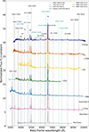 |
Fig. A.1. Raw optical spectra of AT2019aalc. The remarkable lines are indicated with dotted vertical lines. Days relative to the second optical peak are given to the right from each spectra. The SDSS pre-flare spectrum was observed around 11 years before the first optical flare. |
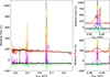 |
Fig. A.2. Pre-flare SDSS spectrum provided by PPXF supplemented by two subplots showing Hα (top right corner) and Hβ (lower right corner). The input spectrum is shown as solid black line, the best stellar and stellar + gas fit are represented as solid red and orange lines, respectively (Cappellari 2023). Additionally, plotted with an arbitrarily chosen offset, one can see the individual gas components (solid blue), total gas emission (solid magenta) and fit residuals (green diamonds) (Cappellari 2023). |
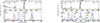 |
Fig. A.3. Examples of the extinction-corrected, continuum- and iron-subtracted over-flare-2 spectra fit using PYQSOFIT. The higher-resolution DBSP spectra were convolved to match with LRIS to allow comparison. The emission lines of interest were modeled with a set of broad and/or narrow Gaussian line components. Left: The LRIS spectrum taken on 2023-06-15, zooming into the Hβ and Hα regions. Right: The DBSP spectrum taken on 2024-05-21, where we also fit the [Fe X] λ6375 high-ionization coronal line as a separate component. |
All Tables
Summary of the optical spectroscopic observations of AT2019aalc. δtf2 is time relative to the optical peak of the second flare.
Emission line properties of AT2019aalc resulted from the fitting procedure. The δt is relative to the optical peak, F(BF) represents the flux of the N IIIλ4640+He IIλ4686 complex, and ncoronal gives the number of the detected high-ionization coronal lines. Superscripts specify which lines are detected, with their labels corresponding to (a) [Fe VII]λ6087, (b) [Fe X]λ6375, (c) [Fe XIV]λ5303, (d) [Fe XII]λ5721, and (e) [Fe XI]λ7892.
All Figures
|
Fig. 1. Pan-STARRS i-band pre-flare image centered on the host galaxy position of the transient event AT2019aalc. The object located to the west of the galaxy core is a foreground star. The green contours represent the pre-flare FIRST radio observations taken at 1.4 GHz. The lowest contour level is drawn at 3σ image noise level corresponding to 0.4 mJy beam−1. Additional positive contour levels increase by a factor of two. The peak brightness is 5.8 mJy beam−1. The red circle points to the Swift-XRT 0.3–10 keV astrometrically corrected position of AT2019aalc, determined using the Swift-XRT data products generator (Evans et al. 2014). Its size indicates the 90% confidence positional error. |
| In the text | |
|
Fig. 2. Optical light curve of AT2019aalc derived from ZTF difference photometry. The transparent markers indicate negative flux (i.e., the flux decreased below the mean flux of the reference images). Two distinct flares can be seen. The second flare peaked 4 years after the first one. The blue vertical line indicates the arrival time of the neutrino event IC191119A associated with the transient. |
| In the text | |
|
Fig. 3. Multiwavelength light curves of AT2019aalc. Bottom plot: X-ray and extinction-corrected and host-subtracted optical/UV. Middle plot: Multifrequency short-baseline radio. Upper plot: Extinction-corrected and host-subtracted IR. Here we show only the positive ZTF fluxes based on the forced photometry results. The dashed gray vertical line indicates the IceCube detection of the high-energy neutrino event IC191119A. The short, purple vertical lines on the top of the bottom panel indicate the peak times of the X-ray flares while the blue ones show the times the main optical r-band flare and later the bumps. The gray ‘S’ letters represent the observing times of the optical spectra. |
| In the text | |
|
Fig. 4. Pre-flare long-term optical light curves of the AGN hosting AT2019aalc starting approximately 14 years before the discovery of the transient in January 2019. The transient is indicated with a blue vertical line. |
| In the text | |
|
Fig. 5. Long-term IR variability of AT2019aalc. The W1−W2 color indicates heated dust as the dominant origin of the IR emission. The second optical flare is accompanied by another IR flaring episode with color change toward the blue. The plotted magnitudes are in the Vega system and have been corrected for extinction but not for host-galaxy contribution, allowing the full evolution between the flares to be visible. |
| In the text | |
|
Fig. 6. Swift-XRT count rate and photon index variability of AT2019aalc during the observing campaign. In most cases are data is well described by a power-law spectral model (black), except during the two recent flaring episodes, where blackbody or combined models are preferred (red). The blackbody temperature is indicated on the red y-axis. |
| In the text | |
|
Fig. 7. Overall Swift-XRT 0.3 − 10 keV spectrum of AT2019aalc. We binned the spectrum to have a minimum of five counts per spectral bin and fit with an absorbed blackbody plus power-law model. |
| In the text | |
|
Fig. 8. Radio spectra of AT2019aalc spanning 3–18 GHz obtained through our ATCA monitoring. We derived a prior radio flare spectrum between 888 MHz and 3 GHz from archival fluxes. The times in the legend are relative to the peak of the second optical flare. |
| In the text | |
|
Fig. 9. Naturally weighted 1.7 GHz EVN+e-MERLIN high-resolution VLBI map of AT2019aalc. The peak brightness is 17.3 mJy beam−1. The gray ellipse in the lower-left corner represents the Gaussian restoring beam. Its parameters are 4.82 mas × 3.7 mas (FWHM) at a major axis position angle of PA |
| In the text | |
|
Fig. 10. Over-flare-2 LRIS spectrum of AT2019aalc in comparison with the SDSS composite spectrum of 10112 Seyfert 1 galaxies published in Pol & Wadadekar (2017) and normalized between 7400 and 7500 Å. The most remarkable lines are shown with vertical lines. The most notable differences are the appearance of the Bowen lines (marked with blue) and the high-ionization coronal lines (marked with green) in the spectrum of AT2019aalc. |
| In the text | |
|
Fig. 11. Second LRIS spectrum of AT2019aalc zoomed in on the He IIλ4686+N IIIλ4640 complex region and compared to those of the BFFs AT2021loi (Makrygianni et al. 2023) and AT2017bgt (Trakhtenbrot et al. 2019), the peculiar transient event AT2019avd (Trakhtenbrot et al. 2020), the repeating TDE AT2020vdq (Somalwar et al. 2025b), and the TDE-Bowen AT2018dyb (Pan et al. 2018). All of the plotted spectra were normalized at 5200 Å. |
| In the text | |
|
Fig. 12. Second LRIS spectrum of AT2019aalc zoomed in on the O IIIλ3133+He IIλ3203 complex region and compared to that of the BFF AT2021loi published by Makrygianni et al. (2023). The spectra were normalized at 5200 Å. |
| In the text | |
|
Fig. 13. [Fe X]λ6375 versus [O III]λ5007 luminosities for (a) ECLEs (Wang et al. 2012; b) variable ECLEs (Yang et al. 2013; c) AT2019aalc (this work); (d) the TDEs AT2019qiz (Short et al. 2023), AT2018dyk, AT2022fpx (Lin et al. 2025), AT2018bcb, AT2021qth and the TDE/QPE AT2022upj; (e) the repeating pTDEs AT2020vdq (Somalwar et al. 2025a) and ASASSN-14ko; (f) the BFFs AT2017bgt, AT2021loi (Makrygianni et al. 2023), F01004-2237; and (g) the BFF candidate AT2019avd (Malyali et al. 2021). A sample of different types of Seyfert galaxies (Gelbord et al. 2009) is plotted as well. The orange line represents a linear fit to the sample, and the orange shaded area represents the 95% prediction interval. The transient sources have clearly higher [Fe X]/[O III] luminosity ratios than the Seyfert sample. |
| In the text | |
|
Fig. 14. Long-term optical light curves of AT2019aalc and three classified BFFs. The light curves indicate that optical re-brightening and bumps may be a common property of BFFs. However, the various sources differ in when these episodes start with regard to the initial flares. |
| In the text | |
|
Fig. 15. Extinction-corrected and host-subtracted SED of the second flare of AT2019aalc as measured around the optical peak. Two blackbody models to the optical/UV (solid curve) and IR data points (dotted curve) were fit separately. A combined fit (black dashed curve) is also shown. |
| In the text | |
|
Fig. 16. Positional coincidences between high-energy neutrino events and the BFFs AT2019aalc and AT2021loi. The blue and red contours represent the 50% and 90%CL containment detailed contours of the high-energy neutrino events IC191119A (left) and IC230511 (right), respectively. The orange box is the 90%CL rectangular containment region. The neutrino best-fit position is shown with a blue point. The optical positions of AT2019aalc (left) and AT2021loi (right) are marked with green star signs. |
| In the text | |
|
Fig. A.1. Raw optical spectra of AT2019aalc. The remarkable lines are indicated with dotted vertical lines. Days relative to the second optical peak are given to the right from each spectra. The SDSS pre-flare spectrum was observed around 11 years before the first optical flare. |
| In the text | |
|
Fig. A.2. Pre-flare SDSS spectrum provided by PPXF supplemented by two subplots showing Hα (top right corner) and Hβ (lower right corner). The input spectrum is shown as solid black line, the best stellar and stellar + gas fit are represented as solid red and orange lines, respectively (Cappellari 2023). Additionally, plotted with an arbitrarily chosen offset, one can see the individual gas components (solid blue), total gas emission (solid magenta) and fit residuals (green diamonds) (Cappellari 2023). |
| In the text | |
|
Fig. A.3. Examples of the extinction-corrected, continuum- and iron-subtracted over-flare-2 spectra fit using PYQSOFIT. The higher-resolution DBSP spectra were convolved to match with LRIS to allow comparison. The emission lines of interest were modeled with a set of broad and/or narrow Gaussian line components. Left: The LRIS spectrum taken on 2023-06-15, zooming into the Hβ and Hα regions. Right: The DBSP spectrum taken on 2024-05-21, where we also fit the [Fe X] λ6375 high-ionization coronal line as a separate component. |
| In the text | |
Current usage metrics show cumulative count of Article Views (full-text article views including HTML views, PDF and ePub downloads, according to the available data) and Abstracts Views on Vision4Press platform.
Data correspond to usage on the plateform after 2015. The current usage metrics is available 48-96 hours after online publication and is updated daily on week days.
Initial download of the metrics may take a while.