| Issue |
A&A
Volume 706, February 2026
|
|
|---|---|---|
| Article Number | A79 | |
| Number of page(s) | 21 | |
| Section | Astrophysical processes | |
| DOI | https://doi.org/10.1051/0004-6361/202555096 | |
| Published online | 02 February 2026 | |
Rethinking mass transfer: A unified semianalytical framework for circular and eccentric binaries
I. Orbital evolution due to conservative mass transfer
1
Anton Pannekoek Institute for Astronomy, University of Amsterdam Amsterdam 1098 XH, The Netherlands
2
School of Physics and Astronomy, Cardiff University Cardiff CF24 3AA, United Kingdom
3
Institute of Astronomy, KU Leuven Celestijnenlaan 200D B-3001 Leuven, Belgium
4
Leuven Gravity Institute, KU Leuven Celestijnenlaan 200D box 2415 3001 Leuven, Belgium
★ Corresponding author: This email address is being protected from spambots. You need JavaScript enabled to view it.
Received:
9
April
2025
Accepted:
15
November
2025
Abstract
Mass transfer (MT) is a fundamental process in stellar evolution. While MT in circular orbits is well studied, observations indicate that it also occurs in eccentric ones, where theoretical models are limited. We present a new semianalytic framework for the secular orbital evolution of mass-transferring binaries that treats stars as either point masses or extended bodies. For the first time, a MT model is applicable to both circular and eccentric orbits and accommodates conservative and nonconservative MT across a broad range of mass ratios and stellar spins. We derived secular orbit-averaged equations describing the orbital evolution by treating MT, mass loss, and angular momentum (AM) loss as perturbations to the general two-body problem. Assuming conservative MT, we compared our results to previous models and validated them against numerical integrations. Our model predicts eccentric post-MT systems in wider orbits than classical results. Compared to other eccentric MT frameworks, the parameter space for orbital widening and eccentricity pumping we find is broader. When extended bodies are accounted for, a stronger semimajor axis and eccentricity growth are obtained at a given mass ratio, and the parameter space is further broadened for orbital widening and eccentricity pumping. Regardless of whether extended bodies are considered, eccentric MT naturally predicts higher eccentricities at longer orbital periods. This correlation has been observed in numerous post-MT systems, and thus eccentric MT provides a robust mechanism for their formation. Our model can be integrated into binary evolution and population synthesis codes to consistently treat conservative and nonconservative MT in arbitrarily eccentric orbits. The applications range from MT on the main sequence to gravitational-wave progenitors.
Key words: celestial mechanics / binaries: close / binaries: general / stars: kinematics and dynamics / stars: mass-loss
© The Authors 2026
 Open Access article, published by EDP Sciences, under the terms of the Creative Commons Attribution License (https://creativecommons.org/licenses/by/4.0), which permits unrestricted use, distribution, and reproduction in any medium, provided the original work is properly cited.
This article is published in open access under the Subscribe to Open model. This email address is being protected from spambots. You need JavaScript enabled to view it. to support open access publication.
1. Introduction
Many binary and multiple-star systems experience at least one MT phase during their evolution (Sana et al. 2012; Moe & Di Stefano 2017). Among the mechanisms of mass exchange such as stellar winds, Roche-lobe overflow (RLOF) stands out for its association with a plethora of observational phenomena. These include X-ray binaries, nova outbursts, cataclysmic variables, Type Ia supernovae, symbiotic stars, and the spin-up of neutron stars. Furthermore, stable MT via RLOF is thought to play a critical role in the formation and evolution of certain populations, such as subdwarf B (sdB) stars (Han et al. 2002, 2003; Podsiadlowski et al. 2008; Heber 2009; Vos et al. 2015, 2017, 2020; Molina et al. 2022), blue stragglers (Geller & Mathieu 2011; Mathieu & Geller 2009), barium (Ba) stars (Jorissen et al. 2019), carbon-rich (CH) and carbon-enhanced metal-poor stars with s-process enhancement (CEMP-s) (Jorissen et al. 2016; Hansen et al. 2016; Sperauskas et al. 2016), gravitational wave (GW) sources (van den Heuvel et al. 2017; Marchant et al. 2021; Picco et al. 2024; Smith & Kaplinghat 2025), and compact double white dwarfs (Woods et al. 2012; Li et al. 2019, 2020).
Current binary evolution models continue to face difficulties in reproducing the orbital properties of many post-MT systems, particularly those with wide and eccentric orbits (Pols et al. 2003; Bonačić Marinović et al. 2008; Dermine et al. 2013; Vos et al. 2015; Oomen et al. 2018, 2020; Molina et al. 2022). Numerical models of binary evolution during RLOF have traditionally neglected orbital eccentricity, assuming that tidal forces universally circularize orbits before the onset of MT (Portegies Zwart & Verbunt 1996; Hurley et al. 2002; Pols et al. 2003; Belczynski et al. 2008; Toonen et al. 2012). This assumption, however, is challenged by observations of interacting binaries with nonzero eccentricities (Petrova & Orlov 1999; Raguzova & Popov 2005) and by inconsistencies in the implementation of tidal prescriptions (Sciarini et al. 2024) or weak tides (e.g., Eldridge 2009; Preece et al. 2022). Moreover, the wide and eccentric nature of many post-MT systems (e.q., see Jorissen et al. 2016; Kawahara et al. 2018; Jorissen et al. 2019; Vos et al. 2020; Molina et al. 2022; Yamaguchi et al. 2024; Shahaf et al. 2024, and references therein) suggests that RLOF may not only preserve, but in some cases even develops, eccentricities in these systems.
Analytical expressions for orbital evolution are crucial for studying the secular evolution of mass-transferring systems in large-scale population studies. Working within the framework established by Hadjidemetriou (e.g., 1969), later authors derived equations describing the secular evolution of orbital elements due to MT via RLOF in eccentric binaries (Sepinsky et al. 2007b, 2009; Dosopoulou & Kalogera 2016a,b). They assumed a delta-function model (the δ-function model) centered at the periapsis of the orbit. This model is physically motivated for systems with extremely high eccentricities, but is invalid for orbits with lower eccentricities. Hamers & Dosopoulou (2019) demonstrated that the equations describing the secular evolution of the orbit are invalid in the case of circular orbits and derived a new set of analytical equations assuming a phase-dependent MT rate. Their updated eccentric mass-transfer model (the emt model) eliminates the problematic behavior at the limit of circular orbits, and it is valid for any eccentricity. This formalism is limited to conservative MT, however.
We present a new semianalytical framework that describes the orbital evolution of mass-transferring binaries. It builds on the physically motivated MT rate derived by Hamers & Dosopoulou (2019). The general mass-transfer model (GeMT model) is designed to address conservative and nonconservative MT scenarios across the full range of orbital eccentricities, including circular orbits. In Sect. 2 we establish the foundation of our approach by treating the effects of MT as perturbations of the instantaneous binary orbit. In Sect. 3 we outline the key components of the model and highlight improvements over previous studies. In Sect. 4 we derive the orbit-averaged equations of the model. In Sect. 5 we explore the model behavior in various limiting cases and compare its predictions with earlier frameworks. In Sect. 6 we apply the model to isolated binaries assuming conservative MT. Finally, we discuss the limitations and implications of our work in Sect. 7, and we conclude in Sect. 8.
2. Perturbed two-body problem. Perturbations during mass transfer
Two-body systems, such as binary stars, are susceptible to gravitational perturbations; tidal dissipation, relativistic corrections, gravitational wave radiation, magnetic fields, inertial forces, mass-loss and/or mass-transfer processes, and others are examples of such agents. All of these physical processes operate as perturbing forces on the general two-body problem (Dosopoulou & Kalogera 2016a), hence the perturbed (actual) orbit of each star diverges from its osculating orbit, that is, the orbit it would have if perturbations were absent.
The perturbing force in principle depends on both the relative position, r, and velocity, ṙ, of the binary components. Therefore, the relative acceleration of the perturbed two-body problem is written as
 (1)
(1)
where f(r,ṙ) is the perturbing force per unit mass. Of course, in the absence of any perturbation f(r,ṙ) = 0 and Eq. (1) describes the general reduced unperturbed two-body problem.
Mass transfer between binary components can occur through various mechanisms yielding such perturbations. During the detached phase, a star may lose mass via stellar winds, with a fraction of the escaping material potentially accreted by the companion. In contrast, if the system transitions into a semidetached phase, the donor star can predominantly transfer mass to its companion, the accretor, through the inner Lagrangian point L1, via RLOF. During RLOF, material is ejected and accreted at specific points and with characteristic velocities, generating reaction forces on both the donor and the accretor. Hereafter, the subscripts “don” and “acc” denote parameters associated with the donor and accretor stars, respectively.
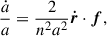
Consider a semidetached binary system. Both stars are assumed to be centrally condensed and spherically symmetric, with masses donated as Mdon and Macc, respectively. The stars rotate around each other, defining an eccentric orbit with semimajor axis a, eccentricity e and period Porb. The total system mass is M = Mdon + Macc, and the mass ratio is defined as q = Mdon/Macc. We assume the binary components rotate uniformly at spin angular velocities Ωdon and Ωacc, parallel to each other and to the orbital angular velocity Ωorb. We note that the magnitude of the vector Ωorb varies over time for eccentric orbits, but it remains directed along the orbital AM vector  , where h ≡ r × ṙ. Specifically,
  and n = 2π/Porb.
Assume that the donor loses mass at a rate Ṁdon from the position rdon (ejection point) relative to its center of mass. Similarly, the accretor gains mass at a rate Ṁacc from the position racc (accretion point) relative to its center of mass. The absolute velocities (i.e, with respect to an inertial reference frame) of the ejected and accreted matter are Wdon and Wacc, respectively. The velocities of the ejected and accreted mass relative to the donor and accretor are wdon = Wdon − dRdon/dt and wacc = Wacc − dRacc/dt, respectively, where dRdon/dt and dRacc/dt denote the absolute velocities of the centers of mass of the donor and accretor. Consequently, a perturbing acceleration acts on the system. Following Hadjidemetriou (1969), Sepinsky et al. (2007b), the perturbing acceleration is written as
 (2)
(2)
where gacc and gdon represent orbital perturbations caused by particles in the MT stream, the terms in the second line represent the change in linear momentum of the accretor and donor caused by mass ejection and accretion, respectively, and the terms in the third line account for the acceleration of the centers of mass of the accretor and donor, resulting from the instantaneous changes in their masses. The derivation is based on the assumption that second- or higher-order terms in ΔMdon and ΔMacc are ignored.
It is important to emphasize that Eq. (2) is generic. In the idealized case of isotropic mass ejection from the donor and accretion onto the companion, such as isotropic stellar winds, the points of ejection and accretion are assumed to coincide with the centers of mass of the two stars (i.e., racc = rdon = 0). In the more general case of anisotropic mass ejection and accretion such as RLOF, however, the points of ejection and accretion are offset from the centers of mass, introducing the perturbing terms proportional to racc and rdon.
In the case of conservative MT, all transferred mass is accreted by the companion, preserving the system’s total mass. In most cases, some transferred mass escapes the system, however. This is referred to as nonconservative MT. We parameterize the fraction of the transferred mass that is accreted as β,1 where 0 ≤ β ≤ 1, and thus,
 (3)
(3)
We note that β = 0 and β = 1 correspond to fully nonconservative and conservative MT, respectively. Moreover, the donor star is losing mass, thus Ṁdon < 0.
In the case of conservative MT, if mass ejection and accretion are isotropic (racc = rdon = 0), the orbital AM is conserved. In the more general case, however, MT is nonconservative, which means that some of the transferred mass escapes the system and carries orbital AM away. Additionally, mass ejection from the donor and accretion onto the companion can be anisotropic, as in the case of RLOF, further altering the orbital AM.
We denote the change in orbital AM due to mass loss as  , and the change due to anisotropic mass ejection and accretion as
  such that
 (4)
(4)
where  and μ = MdonMacc/M. The amount of AM that is carried away by the lost mass can be parametrized in different ways. Following Soberman et al. (1997), we define it to be γ times the specific AM of the binary, such as
 (5)
(5)
The γ parameter is defined relative to the center of mass frame of the system, it can be phase dependent, and it is related to the specific assumptions made about how the mass is lost from the system (Soberman et al. 1997; Parkosidis et al. 2025). In this setting, γ ≥ 0, since Ṁdon < 0, so that  . The
. The  term arises through the perturbing terms proportional to racc and rdon, which account for the impact of the reaction forces on both the donor and the accretor. Thus,
  should be zero in the limit of isotropic mass ejection and accretion, or equivalently in the limit of point masses, namely, racc = rdon = 0.
Considering all perturbations and using Eqs. (2)–(5), we write the total perturbing acceleration as
 (6)
(6)
where the new term in the first line accounts for mass lost from the system and the additional AM it may carry away.
3. Equations of motion
The relative acceleration of the binary components, as influenced by the total perturbation from the MT, is given by substituting Eq. (6) into Eq. (1). The equations are general; they are valid for any eccentricity and can be manipulated to account for different mass exchange and mass loss scenarios. In the following section, we derive the variation of the orbital elements due to MT. First, we present simplifying assumptions that we adopt in our modeling to construct analytically tractable equations. Second, we present a new prescription for the magnitude of the ejection point, rdon, based on the position of the Lagrangian L1 point as a function of various parameters of the system. Furthermore, we demonstrate that using Eq. (6) under the aforementioned basic assumptions, we recover the parameterization given by Eq. (4) and the form of  . Finally, we briefly present the phase-dependent mass-transfer model we used.
3.1. Basic assumptions
Determining the final accretion points and velocities from the initial conditions requires solving the full two-body problem coupled with the dynamics of the MT stream (Lubow & Shu 1975; Sepinsky et al. 2010; Hendriks & Izzard 2023). In general, the transferred mass can: (1) impact directly on the surface of the accretor (direct impact), (2) intersect with itself and form an accretion disk around the accretor, (3) be re-accreted onto the surface of the donor (self-accretion), or (4) escape from the system entirely. In this work, we make two simplifying assumptions to derive analytically tractable equations. The assumptions are listed below:
-
We assume that any gravitational attractions exerted by the particles in the MT stream on the binary components are negligible, thus gdon = gacc = 0.
-
We assume that the donor ejects mass with a relative velocity wdon = ṙ, the accretor accretes mass at wacc = −ṙ and that rdon, racc corotate with the orbit.
The first assumption is valid as long as Mstream ≪ Mdon, Macc (Sepinsky et al. 2007b, 2009; Dosopoulou & Kalogera 2016a,b; Hamers & Dosopoulou 2019). In Sect. 5.1 we show that by adopting the second assumption, the total perturbing acceleration leads to the canonical relation for the change in semimajor axis caused by nonconservative and conservative MT in circular orbits. Simultaneously, it reproduces the canonical expectation that the rate of change of the eccentricity is zero at exactly zero eccentricity.
Applying assumptions 1 and 2, the total perturbation arising due to MT simplifies to
 (7)
(7)
For the vector racc, we investigate two cases where the accretion point is located on the line connecting the two stars, with  . The case of
  applies when the initial velocity of the ejected mass, wdon, is such that the mass stream follows a curved trajectory and lands on the side of the accretor that does not face the donor.
3.2. Ejection point. A new model for the L1 Lagrangian point
Traditionally, the position of the Lagrangian point L1 is defined for circular orbits with synchronously rotating component stars. In eccentric orbits, though, the stars cannot remain synchronous with the orbit at all times due to the time-varying orbital angular velocity. The asynchronous rotation of the donor causes the companion to exert time-dependent tidal forces, resulting in a time-dependent potential. Sepinsky et al. (2007a) demonstrated, however, that this potential can be approximated as quasi-static. In this approximation, the donor shape conforms instantaneously to the quasi-static potential, provided the dynamical timescale of the donor is much shorter than the timescales associated with the orbital angular velocity and the donor rotation, a condition often referred to as the first approximation (Limber 1963).
Following Sepinsky et al. (2007a), the position, X, of the Lagrangian L1 point (relative to the donor center of mass) can be determined by solving the equation
 (8)
(8)
where XL is expressed in units of the instantaneous orbital separation (i.e., XL = X/r), fdon represents the angular spin velocity of the donor normalized to the orbital angular velocity at periapsis, so that
 (9)
(9)
and
 (10)
(10)
quantifies the deviation of the donor spin velocity from the orbital angular velocity at periapsis as a function of the eccentricity e and eccentric anomaly ℰ. 𝒜(fdon, e, ℰ) reaches its maximum for e approaching 1 at ℰ = π, while it is minimal for e = 0, (see Sepinsky et al. 2007a, Fig. 3). We note that we choose the eccentric anomaly to express 𝒜(fdon, e, ℰ), however other angle parameters, such as true anomaly, are equally valid parameters.
Similar to Sepinsky et al. (2007b), we solve for the periapsis of the orbit, such as 𝒜(fdon, e, ℰ = 0), and thus Eq. (8) is written as
 (11)
(11)
We fit a prescription, XL1(fdon, q, e), to the numerical solutions of Eq. (11), such as XL = XL1(fdon, q, e) and therefore, the phase-dependent position of L1 in natural units is
 (12)
(12)
The XL1(fdon, q, e) function gives the position of the L1 point at the periapsis of the binary orbit in units of the instantaneous distance between the two stars, and it is given explicitly in Appendix B. Hereafter, we refer to our prescription as the “global-L1” fit. We note that an alternative, overall less accurate, fit to the numerical solution of Eq. (11) is provided by Sepinsky et al. (2007b, see their Eq. (A15)). A comparison of the two is given in Fig. B.3.
Solving Eq. (8) is nontrivial. Hamers & Dosopoulou (2019) proposed two analytical solutions based on distinct limiting assumptions: negligible donor spin velocity, that is, fdon ≈ 0, and large mass ratio, namely, q ≫ 1. These solutions are hereafter referred to as the “low-fdon” and “high-q” models, respectively. In this work, we use the global-L1 prescription for the position of L1, which is applicable across the entire range of mass ratios while retaining sensitivity to the spin velocity of the donor.
In Fig. 1 we compare the global-L1 fit predictions to the numerical solutions of Eq. (11) for e = 0.3 and varying donor spins fdon. As q increases, the position of the L1 point shifts further from the donor center of mass. Conversely, higher donor spins bring the L1 point closer to the donor. This behavior aligns with expectations, as the centrifugal acceleration (captured by 𝒜(fdon, e, ℰ)) increases with fdon, making it easier for surface material to escape. The high-q model is independent of q and breaks down for subsynchronous donors, incorrectly placing L1 behind the accretor. The low-fdon is independent of fdon and becomes increasingly inaccurate as fdon increases. This model effectively represents the limiting case of the global-L1 model at fdon = 0.
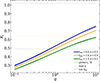 |
Fig. 1. Position of the L1 point relative to the donor center of mass at the periapsis of the binary orbit in units of the instantaneous binary separation. The thick lines show the numerical solutions of Eq. (11). The dotted, dashed, and thin lines illustrate the high-q, low-fdon, and global-L1 models, respectively. Blue, orange, and green correspond to fdon = 0.5, 1.0, and 1.5, respectively, and e = 0.3 for all models. The low-fdon prescription is independent of fdon. |
In Fig. 2 we compare our global-L1 model to the high-q and low-fdon models by tracking the predicted position of the L1 point over one orbital cycle for different eccentricities. In the high-q model, the location of L1 is independent of the orbital phase, and the approximation breaks down for circular orbits with synchronous donors, incorrectly placing L1 in the center of the accretor, and for fdon < 1, even behind it. The low-fdon model is more accurate. In this case, the location of L1 itself varies during one orbit, and it is always between the binary components, but no information about the donor rotation is included. For circular orbits, the global-L1 model provides an accurate position of the L1 point (the dashed blue line completely overlaps the thick blue line), while both low-fdon and high-q models show visible offsets. Additionally, for any e > 0 our prescription is less accurate during orbital phases when the MT rate is low, while it becomes more accurate close to the periapsis of the orbit where the MT rate is expected to be maximum. A detailed discussion is presented in Appendix B.
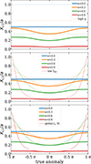 |
Fig. 2. Position of the L1 point relative to the donor center of mass in units of the semimajor axis a for q = 1 and fdon = 1 as a function of the true anomaly. The thick lines are the numerical solutions of Eq. (8). From top to bottom, the dotted, dashed, and thin lines illustrate the high-q, low-fdon, and global-L1 models, respectively. Blue, orange, green and red correspond to e = 0.0, 0.3, 0.6, and 0.9, respectively. |
3.3. Orbital-element variations during mass transfer
A perturbation induced on a binary system can give rise to changes in the Keplerian orbit elements. We highlight that Eq. (7) does not contain any components that are out of the orbital plane. A perturbing acceleration of this form does not change the inclination of the orbit i, nor the longitude of the ascending node Ω. The semimajor axis, a, the eccentricity, e, and the argument of periapsis, ω, evolve, however.
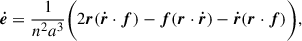
Following Hadjidemetriou (1963), Dosopoulou & Kalogera (2016a), we calculate the evolution of the orbital elements as
 (13)
(13)
 (14)
(14)
 (15)
(15)
where ![Mathematical equation: $ \boldsymbol{e} = n^{-2} a^{-3} [\boldsymbol{r} (\boldsymbol{\dot{r}} \cdot \boldsymbol{\dot{r}}) - \boldsymbol{\dot{r}}(\boldsymbol{r} \cdot \boldsymbol{\dot{r}})] - \hat{\boldsymbol{r}} $](/articles/aa/full_html/2026/02/aa55096-25/aa55096-25-eq27.gif) and
and  .
.
In principle, the derivation of Eqs. (13)–(15) assumes that the total mass of the binary is constant. The effects of mass loss and AM loss are explicitly incorporated into the perturbing acceleration ftotal, however. Specifically, consider a binary system with a constant total mass and assume that an external force per unit mass, as described by Eq. (7), acts on the system. Under these conditions, the osculating orbit would undergo the same changes as it does when the total mass varies (Hadjidemetriou 1963; Dosopoulou & Kalogera 2016a).
In Appendix A we show that using Eqs. (13), (14), and (7), we recover
 (16)
(16)
Moreover, Eqs. (4) and (16) show that
 (17)
(17)
and in the limit of point masses (i.e., racc = rdon = 0),  , thus Eq. (16) reduces to Eq.(5) as expected.
We emphasize that for isotropic ejection and accretion (i.e., racc = rdon = 0), Jorb is an integral of motion both in fully conservative MT (β = 1) and in the nonconservative case if the ejected mass carries no net AM (γ = 0). The orbital evolution differs, however, because when β < 1, the total system mass varies, even though the orbital AM does not. Essentially, γ = 0 represents an idealized scenario in which the total mass of the system varies in such a way that it does not carry away net AM; such an example would be an isotropic wind originating from the center of mass of the system. In this setup, the orbital AM can evolve only if mass is lost from the system.2 Mass can be lost from the system without removing AM (γ = 0), however. Finally, the derivation of Eq. (16) is independent of the prescription of the mass-loss rate.
3.4. Phase-dependent mass transfer rate
In a circular binary with synchronously rotating stars, the Roche lobe radius is phase-independent, and it is given in good approximation by the fit of Eggleton (1983),
 (18)
(18)
If the physical radius of the donor overflows the Roche lobe radius (i.e., ΔR = Rdon − RLc ≥ 0), then MT occurs. If ΔR < 0, no mass is transferred. The MT rate is extremely sensitive to the extent to which the physical radius overflows the Roche lobe radius.
In this work, we adopt the phase-dependent MT model developed by Hamers & Dosopoulou (2019). In this model, the MT rate is well-defined at high and low eccentricities, including circular orbits, where MT occurs continuously throughout the orbit. Below, we summarize the key aspects of the model relevant to interpreting our results; a more detailed description can be found in Hamers & Dosopoulou (2019).
The model is based on the magnitude of ΔR. By assuming a polytropic equation of state for the donor (with a polytrope index np = 1.5) and applying Bernoulli’s equation (Paczyński & Sienkiewicz 1972; Edwards & Pringle 1987), the MT rate is given by
 (19)
(19)
where Ṁdon,0 represents a phase-independent MT rate, and
 (20)
(20)
is an approximation for the instantaneous Roche lobe radius.
Using r(ℰ) = a(1 − ecosℰ), the MT rate is written as
![Mathematical equation: $$ \begin{aligned} \dot{M}_{\rm don} = \dot{M}_{\rm don,0}[1-x(1-e\cos {\mathcal{E} })]^3, \; \text{ where} \; x\equiv \frac{R_{\rm L}^c}{{R_{\rm don}}}\cdot \end{aligned} $$](/articles/aa/full_html/2026/02/aa55096-25/aa55096-25-eq35.gif) (21)
(21)
As a result, the MT rate is expected to be maximum at periapsis and minimum at apoapsis, where the instantaneous Roche lobe radius is minimum and maximum, respectively.
During one orbit, for a given e and x, a system can transfer no mass at all (no RLOF), can transfer throughout the whole orbit (full RLOF), or can transfer during part of the orbit (partial RLOF). Figure 3 visually depicts the three scenarios on the e − x plane. Additionally, for circular orbits, there is only full RLOF or no RLOF, which correspond to x < 1 or x ≥ 1, respectively. This is to be expected because for a circular orbit, x is an alternative way to measure how much or if the physical radius Rdon overflows the Roche lobe radius RLc.
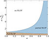 |
Fig. 3. Graphical representation of the mass-transfer regimes based on the mass-transfer rate formulation by Hamers & Dosopoulou (2019). The white region indicates no mass transfer, i.e. no RLOF. The light blue region corresponds to partial RLOF, where mass transfer occurs during part of the orbit. The light brown region represents full RLOF, with continuous mass transfer throughout the entire orbit. |
The part of the orbit in which MT takes place is given by −ℰ0 < ℰ < ℰ0. For MT occurring over the entire orbit (full RLOF), ℰ0 = π. For MT limited to a portion of the orbit (partial RLOF), ℰ0 is given by
 (22)
(22)
We note here that ℰ0 essentially defines the limits of the integration when we calculate the orbit-averaged MT rate (see below Sect. 4), because the MT rate is assumed to be zero for ℰ < −ℰ0 and ℰ > ℰ0.
Assuming Ṁdon,0,e and x are constant over one orbit,  becomes
![Mathematical equation: $$ \begin{aligned} \ddot{M}_{\rm don} = -3nxe\dot{M}_{\rm don,0}[1-x(1-e \cos {\mathcal{E} })]^2 \frac{\sin \mathcal{E} }{1-e\cos \mathcal{E} }\cdot \end{aligned} $$](/articles/aa/full_html/2026/02/aa55096-25/aa55096-25-eq38.gif) (23)
(23)
4. Orbit-averaged equations
Our aim is to retrieve the secular evolution of the orbital elements, thus we remove periodic terms by averaging over one orbit. We define orbit-averaged quantities in the following way,
 (24)
(24)
where (…) denotes the quantity to be averaged.
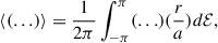
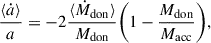
The perturbing acceleration of Eq. (7), which is responsible for the variation of the orbital elements, is inversely proportional to the MT timescale Mdon/Ṁdon = τṀdon. When  , we can assume that systematic parameters, such as Macc, Mdon, a, e, x, and so on are approximately constant over one orbit (i.e., adiabatic approximation). We substitute Eq. (21) into Eq. (7) and from Eqs. (24), (13) to (15) we derive the orbit-averaged equations of motion in the adiabatic regime as
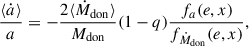
![Mathematical equation: $$ \begin{aligned} \frac{\langle \dot{a} \rangle }{a}&= -\frac{2 \dot{M}_{\rm don,0}}{M_{\rm don}} \Biggl [ \Biggl (1-\beta q-(1-\beta )\frac{(\gamma +\frac{1}{2})q}{1+q}\Biggr )f_{a}(e,x) \nonumber \\&\quad + X_{\rm L1}(f_{\rm don},q,e) g_{a}(e,x) \pm \beta q \frac{r_{\rm acc}}{a} h_{a}(e,x) \Biggr ],\\ \langle \dot{e} \rangle&= -\frac{2 \dot{M}_{\rm don,0}}{M_{\rm don}} \Biggl [ \Biggl (1-\beta q-(1-\beta )\frac{(\gamma +\frac{1}{2})q}{1+q}\Biggr )f_{e}(e,x) \nonumber \\&\quad + X_{\rm L1}(f_{\rm don},q,e) g_{e}(e,x) \pm \beta q \frac{r_{\rm acc}}{a} h_{e}(e,x) \Biggr ],\end{aligned} $$](/articles/aa/full_html/2026/02/aa55096-25/aa55096-25-eq41.gif) (25)
(25)
 (26)
(26)
where  , and he(e, x) are dimensionless functions given explicitly in Appendix E. The negative sign in front of the term associated with the accretion point corresponds to
  , while the positive sign to
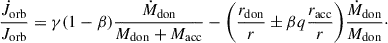
  . The dimensionless functions are equivalent to those derived by Hamers & Dosopoulou (2019). It is important to note that there is a typo in Hamers & Dosopoulou (2019, their Eq. (52)). As a result, we recommend the verification of the he(e, x) integral before using the emt model. Furthermore, Hamers et al. (2021) present an ad hoc extension of the emt model to nonconservative MT. The effects of mass loss and AM loss are not taken into account when computing the evolution of the orbital elements, however (see Parkosidis et al. 2025).
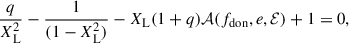
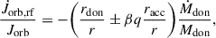
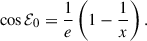
As described in Sect. 3.4, the MT rate contains a periodic term and a phase-independent MT rate (Eq. (21)). The periodic term is a consequence of the distance between the stars varying over one orbit (see Eq. (21)). When applying Eqs. (25)–(27) within detailed or rapid stellar evolution codes, one may not have direct access to the normalization parameter Ṁdon,0. For this reason, we re-express the equations in terms of the orbit-averaged MT rate ⟨Ṁdoon⟩ (in the adiabatic regime). The orbit-averaged MT rate is defined via Eqs. (21) and (24) as
![Mathematical equation: $$ \begin{aligned} \langle \dot{M}_{\rm don} \rangle&\equiv \frac{1}{2 \pi }\int _{-\pi }^{\pi } \dot{M}_{\rm don,0} [1-x(1-e\cos {\mathcal{E} })]^3 (\frac{r}{a}) d \mathcal{E} \nonumber \\&= \dot{M}_{\rm don,0} f_{\dot{M}_{\rm don}}(e,x), \end{aligned} $$](/articles/aa/full_html/2026/02/aa55096-25/aa55096-25-eq46.gif) (27)
(27)
where  is a dimensionless function acting as a normalization factor. We note that the limits of integration are effectively determined by ℰ0 via Eq. (22), since the MT rate is assumed to vanish outside the range −ℰ0 < ℰ < ℰ0. Consequently, the secular evolution equations of motion are given as
![Mathematical equation: $$ \begin{aligned} \frac{\langle \dot{a} \rangle }{a}&= -\frac{2 \langle \dot{M}_{\rm don} \rangle }{M_{\rm don}} \frac{1}{f_{\dot{M}_{\rm don}}(e,x)} \Biggl [ \Biggl (1-\beta q-(1-\beta )\frac{(\gamma +\frac{1}{2})q}{1+q}\Biggr )f_{a}(e,x) \nonumber \\&\quad + X_{\rm L1}(f_{\rm don},q,e) g_{a}(e,x) \pm \beta q \frac{r_{\rm acc}}{a} h_{a}(e,x) \Biggr ],\\ \langle \dot{e} \rangle&= -\frac{2 \langle \dot{M}_{\rm don} \rangle }{M_{\rm don}} \frac{1}{f_{\dot{M}_{\rm don}}(e,x)} \Biggl [ \Biggl (1-\beta q-(1-\beta )\frac{(\gamma +\frac{1}{2})q}{1+q}\Biggr )f_{e}(e,x) \nonumber \\&\quad + X_{\rm L1}(f_{\rm don},q,e) g_{e}(e,x) \pm \beta q \frac{r_{\rm acc}}{a} h_{e}(e,x) \Biggr ],\\ \langle \dot{\omega } \rangle&= 0. \end{aligned} $$](/articles/aa/full_html/2026/02/aa55096-25/aa55096-25-eq48.gif) (28)
(28)
Furthermore, ⟨Ṁdoon⟩ is assumed to be known and constant throughout a single orbit, serving as a free parameter within the model. It is important to note that ⟨Ṁdoon⟩ can change over long timescales due to the donor response to MT or as a result of stellar evolution. Therefore, ⟨Ṁdoon⟩ should ideally be calculated self-consistently (e.g., Rocha et al. 2025). Nevertheless, the qualitative behavior of Eqs. (29)–(31) is independent of the exact choice of ⟨Ṁdoon⟩.
We implement the secular equations of motion (Eqs. (29)–(31)) into a code named General Mass Transfer (GEMT). To ensure that our equations are only applied in the parts of the parameter space in which MT occurs, we introduce three stopping conditions. Specifically, we do not evolve the orbital elements if (1) a system detaches (i.e., is located in the no RLOF regime in Fig. 3; mathematically RLc(1 − e) > Rdon), (2) the radius of the donor is equal to or larger than the periastron distance (i.e., the system merges; mathematically Rdon ≥ a(1 − e)), and (3) the orbit becomes parabolic (mathematically e > 0.99). In the following section, we examine the behavior of the GeMT model in various limiting cases and compare its predictions with those of earlier models.
5. Properties of the orbit-averaged equations
In this section, we examine the secular rates of change for the semimajor axis a (Eq. (29)) and eccentricity e (Eq. (30)) under various limiting conditions. Section 5.1 demonstrates that the GeMT model reproduces the classical RLOF results in the limit of circular orbits and point masses. Sections 5.2 and 5.3 present the predicted orbital evolution for circular and eccentric orbits, respectively. Moreover, we compare the predictions of the GeMT model with the results derived in the limit of point masses, as well as with the δ-function and emt models. Hereafter, when referring to the case of extended bodies (i.e., rdon, racc ≠ 0), we implicitly include the impact of anisotropic mass ejection from the donor and accretion onto the companion on the secular evolution. Considering the emt model, we adopt the default low-fdon prescription throughout this work. Moreover, we adopt cos(ϕP) = − 1 for the δ-function model throughout this work. In Table 1 we summarize the initial conditions at the onset of RLOF for the different examples presented.
Initial conditions at the onset of RLOF.
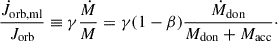
5.1. Point masses and circular orbits
In the classical picture of RLOF, the orbit is circular, and the binary components are modeled by point masses (see Postnov & Yungelson 2014). Following Soberman et al. (1997) and using the orbital AM,  , the change of the semimajor axis of the orbit is given by
 (29)
(29)
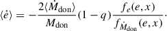
In the limit of point masses (i.e., rdon = racc = 0), the orbit-averaged equations of motion (Eqs. (29) and (30)) reduce to
![Mathematical equation: $$ \begin{aligned} \frac{\langle \dot{a} \rangle }{a}&= -\frac{2 \langle \dot{M}_{\rm don} \rangle }{M_{\rm don}} \frac{f_{a}(e,x)}{f_{\dot{M}_{\rm don}}(e,x)} \Biggl [ 1-\beta q-(1-\beta )\frac{(\gamma +\frac{1}{2})q}{1+q} \Biggr ],\end{aligned} $$](/articles/aa/full_html/2026/02/aa55096-25/aa55096-25-eq53.gif) (30)
(30)
![Mathematical equation: $$ \begin{aligned} \langle \dot{e} \rangle&= -\frac{2 \langle \dot{M}_{\rm don} \rangle }{M_{\rm don}} \frac{f_{e}(e,x)}{f_{\dot{M}_{\rm don}}(e,x)} \Biggl [ 1-\beta q-(1-\beta )\frac{(\gamma +\frac{1}{2})q}{1+q} \Biggr ]. \end{aligned} $$](/articles/aa/full_html/2026/02/aa55096-25/aa55096-25-eq54.gif) (31)
(31)
Furthermore, if the orbit is circular (see Appendix C), the resulting secular change rates simplify to
![Mathematical equation: $$ \begin{aligned} \frac{\langle \dot{a} \rangle }{a}&= -\frac{2 \langle \dot{M}_{\rm don} \rangle }{M_{\rm don}} \Biggl [ 1-\beta q-(1-\beta )\frac{(\gamma +\frac{1}{2})q}{1+q} \Biggr ].\end{aligned} $$](/articles/aa/full_html/2026/02/aa55096-25/aa55096-25-eq55.gif) (32)
(32)
 (33)
(33)
Consequently, in the limit of point masses and circular orbits, the GeMT model reproduces the canonical relation for the rate of change of the semimajor axis, given by Eq. (32). The latter is widely used in studies of nonconservative MT in circular orbits (e.g. Soberman et al. 1997; Postnov & Yungelson 2014). Notably, in the limit of ℰ0 → π, ⟨ė⟩ ∝ e, indicating that an initially circular orbit, which mathematically is e = 0, remains circular. On the other hand, if the system has some seed eccentricity (i.e., e ≠ 0), we expect ⟨ė⟩ ≠ 0.
For β = 1, Eq. (35) reduces to
 (34)
(34)
which is the canonical relation used in studies of conservative MT (e.g., Pringle & Wade 1985; Hurley et al. 2002; Kashi & Soker 2018). According to Eq. (37), the orbit expands when the donor is less massive than the accretor, and contracts otherwise. Consequently, the evolution of the semimajor axis is consistent with the conservation of  .
.
We note that the δ-function model for eccentric RLOF used in numerous studies (Sepinsky et al. 2007b, 2009; Dosopoulou & Kalogera 2016a,b; Rocha et al. 2025) is invalid in this regime. Specifically, at e = 0.0, the eccentricity derivative is nonzero, becoming negative when q > 1 and positive when q < 1, as shown by Hamers & Dosopoulou (2019).
5.2. Circular orbits and the effect of the spin velocity of the donor
For extended bodies, rdon = XL1(fdon, q, e)r, and we assume that  . In the limit of circular orbits (see Appendix C), the GeMT model simplifies to
![Mathematical equation: $$ \begin{aligned} \frac{\langle \dot{a} \rangle }{a}&= -\frac{2 \langle \dot{M}_{\rm don} \rangle }{M_{\rm don}} \Biggl [ \Biggl (1-\beta q-(1-\beta )\frac{(\gamma +\frac{1}{2})q}{1+q}\Biggr ) \nonumber \\&+ X_{\rm L1}(f_{\rm don},q,e \rightarrow 0) \pm \beta q \frac{r_{\rm acc}}{a} \Biggr ],\end{aligned} $$](/articles/aa/full_html/2026/02/aa55096-25/aa55096-25-eq60.gif) (35)
(35)
 (36)
(36)
where XL1(fdon, q, e) is given explicitly in Appendix B. From Eq. (38), we observe that the rate of change of the semimajor axis is independent of x (see also Fig. 3). Notably, this rate retains information about the spin angular velocity of the donor (fdon) star.
In Fig. 4 we show the rate of change of the semimajor axis (Eq. (38)) as function of mass ratio q varying fdon. Additionally, we compare these results with the rates predicted by the GeMT model in the limit of point masses, as well as the δ-function and the emt models. Red regions indicate orbital shrinkage, while blue regions represent orbital widening, with the color intensity reflecting the magnitude of the rate: deeper red and blue correspond to stronger shrinkage and widening, respectively.
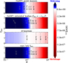 |
Fig. 4. Secular change rate of the semimajor axis as a function of the mass ratio q and the level of synchronism fdon of the donor in the limit of circular orbits. From top to bottom, GeMT model in the limit of point masses, extended bodies for |

In the point-mass limit and δ-function models, the transitional mass ratio qtrans, a separating orbital widening and shrinkage occurs at equal masses (qtrans, a = 1) and is independent of the spin velocity of the donor. This result is expected since, in the δ-function model, the terms associated with rdon, racc are proportional to the eccentricity e and vanish as e → 0, regardless of whether extended bodies are considered. Consequently, the model simplifies to the canonical relation for the semimajor axis evolution in this regime, given by Eq. (37). The color intensity indicates, however, that the δ-function model predicts weaker evolution of the semimajor axis across all mass ratios. The canonical relation for the semimajor axis evolution (Eq. (37)) and δ-function model would be exactly equivalent only if ⟨Ṁdoon⟩ in Eq. (37) is interpreted as ⟨Ṁdoon⟩ = Ṁ0/(2π) (see also Sect. 5 in Sepinsky et al. 2007b), which applies only to circular orbits (see Appendix D).
The GeMT model takes into account the position of the L1 (global-L1 model) point, and the orbital evolution deviates from the classical RLOF picture. Specifically, the parameter space for orbital widening as well as the intensity of the blue region increase. qtrans, a shifts to higher values, e.g. for synchronous donors (fdon = 1.0), our model predicts qtrans, a ≈ 1.53. Furthermore, increasingly subsynchronous donors result in higher qtrans, a and vice versa; with qtrans, a ≈ 1.57 for fdon = 0.0 and qtrans, a ≈ 1.44 for fdon = 2.0, respectively. Finally, the bluer color shows a stronger orbital widening compared to the point-mass and δ-function models.
The emt model also predicts qtrans, a > 1, but unlike the GeMT model, the rate of change of the semimajor axis is independent of the donor’s spin velocity. This is because the low-fdon prescription used for the position of the L1 point assumes fdon ≈ 0. In summary, for circular orbits, the semimajor axis in the emt model is entirely independent of fdon. Essentially, the emt model is a subset of the GeMT model under the specific condition of nonrotating donors (fdon = 0).
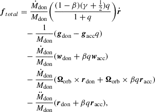
5.3. Eccentric orbits
For nonzero eccentricities, the secular rates of change of the semimajor axis a and eccentricity e are determined by Eqs. (29) and (30). In Figs. 5 and 6, we show the aforementioned rates in the limit of conservative MT as functions of the mass ratio q and the eccentricity e, respectively. Additionally, we compare these results with the rates predicted by the GeMT model in the limit of point masses, as well as with those from the δ-function and the emt models. For nonzero eccentricities, the terms associated with ejection and accretion points (rdon, racc) in the δ-function model are nonzero. Consequently, we employ the prescription of the L1 point XL1, sep(fdon, q, e) as derived by Sepinsky et al. (2007b, see their Eq. (A15)). Specifically, |rA1, P|=XL1, sep(fdon, q, e)a(1 − e).
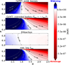 |
Fig. 5. Secular change rate of the semimajor axis in the limit of conservative mass transfer as a function of mass ratio q and eccentricity e. From top to bottom, GeMT model in the limit of point masses, extended bodies for |

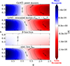 |
Fig. 6. Similar to Fig. 5, but the color gradient now illustrates the secular change rate of the eccentricity. |
In the limit of point masses, the GeMT model predicts that the orbit expands when q < 1 and shrinks when q > 1, independent of e (Fig. 5). When we account for extended bodies, however, the parameter space for orbital widening and shrinkage changes. Specifically, the GeMT model predicts that for lower eccentricities, the transitional mass ratio, qtrans, a, shifts to higher values and vice versa for higher eccentricities. The δ-function model also shows a decrease in qtrans, a with increasing eccentricity for nonzero eccentricities. The predicted qtrans, a values are significantly lower, however. Additionally, the color gradient in the δ-function model suggests a weaker evolution of the semimajor axis compared to the GeMT model. Notably, in the limit of conservative MT (β = 1) and nonrotating donors (fdon = 0.0) the GeMT and the emt models are equivalent.
The GeMT model predicts an eccentricity-evolution parameter space that closely resembles that of the semimajor axis (Figs. 6 and 5). In the limit of point masses, ė is positive for q < 1 and negative for q > 1, independent of e. When extended bodies are considered, the parameter space for eccentricity pumping broadens. Specifically, the transitional mass ratio, qtrans, e, shifts to higher values, a trend more prominent for lower eccentricities. In contrast, the δ-function model shows that qtrans, e remains largely independent of e, with the eccentricity-pumping regime confined to q ≤ 0.74. Additionally, the color gradient suggests a weaker evolution of the eccentricity compared to the GeMT model across all mass ratios and eccentricities. Finally, for β = 1 and fdon = 0.0 the GeMT and the emt models are equivalent.
6. Applications. Conservative mass transfer
In this section, we examine the orbital evolution of isolated binary systems undergoing conservative RLOF (β = 1). Using the GeMT code, we numerically integrate Eqs. (29) and (30). Here, we neglect additional physical processes such as tides or stellar evolution to isolate the effects of MT via RLOF. For simplicity, we treat the stars as rigid spheres and assume that both the donor radius Rdon and the accretor radius (or the outer edge of the accreting disc) racc remain constant throughout the integration.
6.1. Comparison to different mass-transfer frameworks
We consider a system with initial parameters: Mdon = 8 M⊙, Macc = 1.4 M⊙, Rdon = 10 R⊙, racc = 0.01 R⊙, a = 1 au and e = 0.92, equal to the example system of Hamers & Dosopoulou (2019). In this configuration, the accretor represents a neutron star. The donor initiates RLOF near periapsis at x ≈ 11.4. We assume ⟨Ṁdoon⟩ = 10−8 M⊙ yr−1 for the emt and GeMT models, and Ṁ0 = 10−8 M⊙ yr−1 for the δ-function model. For a direct comparison with previous models, we set  for the GeMT model. The evolution of the system is presented in Fig. 7.
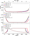 |
Fig. 7. Evolution of the semimajor axis (top), eccentricity (middle), mass ratio q, and angle ℰ (bottom) as a function of time during mass transfer. The dashed black and gray lines correspond to the emt and δ-function (fdon = 1.0) models, respectively. The orange, blue and red lines correspond to the GeMT model, for subsynchronous (fdon = 0.0), synchronous (fdon = 1.0) and supersynchronous donors (fdon = 2.0), respectively. In the bottom panel, the two horizontal dotted lines indicate ℰ0 = π and q = 1. |
Initially, the system undergoes partial RLOF, during which both the semimajor axis and the eccentricity decrease across all models. In the emt and GeMT models, the orbit becomes almost circular and the system transitions to full RLOF by t ≈ 100 Myr. Meanwhile, the orbit keeps shrinking until q ≈ 1.5 at t ∈ [200, 250] Myr. Beyond this point, the orbit begins to expand, and the system transitions back to partial RLOF at t ≈ 500 Myr. This transition marks the point that the eccentricity starts increasing again. Figure 8 illustrates how the system transitions between the partial and full RLOF regimes during its evolution.
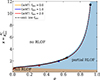 |
Fig. 8. Evolution of the systems presented in Fig. 7 in the e − x plane for subsynchronous (fdon = 0.0), synchronous (fdon = 1.0), and supersynchronous donors (fdon = 2.0). The circles and triangles indicate the initial and final positions of the systems, respectively. |
Slower donor rotation leads to greater orbital widening and eccentricity growth because lower fdon places the L1 point farther from the donor (see Fig. 1), yielding to larger initial ȧ/a and ė (see Fig. 5). Consequently, for rotating donors with lower spin (i.e., lower fdon), the system evolves into wider and more eccentric orbits. Finally, the GeMT model reproduces the results of the emt model for fdon = 0 (limit of a nonrotating donor).
The evolution predicted by the δ-function model is significantly different from other models (see also Sect. 7.3 and Appendix D). Initially, both the semimajor axis and the eccentricity decrease, with mass reversal occurring at t ≈ 330 Myr. Following mass reversal, the orbit slowly widens and eccentricity slowly increases. The change rates for both parameters are notably weaker than in the GeMT model, however. Unlike other predictions, the orbit remains highly eccentric, with emin ⪆ 0.9.
6.2. Formation of wide post-MT binaries in eccentric orbits
We consider a donor Mdon = 1.1 M⊙ in a nearly circular orbit of e = 0.001. The initial semimajor axis and accretor mass are ai = 1.08, 1.11, 1.14 au and Macc, i = 0.7, 0.8, 0.9 M⊙, respectively. In all three configurations, the donor fills its Roche lobe around the tip of the red giant branch (RGB), when Rdon ≈ 102 R⊙ (initially, x ≈ 0.95), and initiates MT; late Case B examples. Temmink et al. (2023) showed that for such mass ratios, the MT proceeds in a stable manner (they assumed a point mass accretor). During the ascent of the RGB, the donor develops a degenerate helium core that grows in mass until the occurrence of the helium flash when the core mass Mc ≈ 0.47 M⊙ (Han et al. 2002), while the accretor is still on the main sequence. In contrast to Sect. 6.1, we track the orbital evolution assuming point masses under the assumption that the AM stored in the stars in negligible compared to the orbital AM. Under the assumption of conservative MT and point masses, our model is equivalent to the emt model. We assume ⟨Ṁdoon⟩ = 10−8 M⊙ yr−1. In addition, we follow the orbital evolution under the classical RLOF framework (dotted lines in Fig. 9), assuming circularization at the onset of MT. The initial semimajor axis is set equal to the original orbital separation at periapsis,3 that is, acirc = a(1 − e). The evolution of the system is presented in Fig. 9.
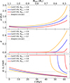 |
Fig. 9. Similar to Fig. 7, but now for an initially nearly circular binary (e = 0.001). The orange, blue, and red lines correspond to the GeMT model for a = 1.08, 1.11, and 1.14 au and Macc = 0.7, 0.8, and 0.9 M⊙, respectively. In the top panel, the dotted lines illustrate the classical analytic expectation that |

In the classical RLOF model, the orbit initially shrinks across all three models (dotted lines) until mass reversal at t ∈ [10 − 20] Myr, after which it widens. By the end of the evolution, all three post-MT systems are circular with longer orbital periods than before MT. For the GeMT model, all three systems initially undergo full RLOF, during which the semimajor axis decreases, similar to the classical model. The orbital evolution diverges when the models transition from full to partial RLOF, however. The semimajor axis changes more rapidly than in the classical case, and the eccentricity increases. Figure 10 shows how the systems alternate between partial and full RLOF during its evolution.
Systems with a higher initial accretor mass Macc (i.e., lower initial mass ratios q) evolve to wider, more eccentric final orbits (Fig. 9). These systems initiate RLOF with q closer to the critical qtrans, a = qtrans, e = 1 (bottom panel in Fig. 9), while the total transferred mass is the same across all models. Consequently, they spend a larger fraction of their evolution in the orbital widening and eccentricity pumping regions than systems with larger initial q (see also Figs. 5 and 6).
In summary, the δ-function framework yields the weakest secular evolution among the three models; in Sect. 7.3 and Appendix D we show why this is the case. Moreover, the emt model is a subset of the GeMT in the limit of conservative MT (β = 1) and nonrotating donors (fdon = 0). In the GeMT framework, for point masses under conservative MT, the secular changes in semimajor axis and eccentricity are correlated: Orbits either widen while becoming more eccentric or shrink while circularizing.
7. Discussion
7.1. Model limitations
Working in the framework established by Hadjidemetriou (1969) and by adopting the assumptions outlined in Sect. 3.1, we present a novel, semianalytical framework for describing the secular orbital evolution of semidetached systems undergoing RLOF. As Hamers & Dosopoulou (2019) previously emphasized, the validity of assumption 2 (imposing ejection (wdon = ṙ) and accretion velocities (wacc = − ṙ)) requires careful evaluation (see Luk’yanov 2008). Notably, by adopting this assumption, we recover the canonical relation for changes in the semimajor axis due to both nonconservative and conservative MT in the limit of circular orbits. While our assumptions are physically motivated, future studies are essential to thoroughly assess their validity in other regimes.
Hydrodynamical simulations of mass-transferring binaries via RLOF (e.g., Regös et al. 2005; Church et al. 2009; Lajoie & Sills 2011; van der Helm et al. 2016; Bobrick et al. 2017) would be important in estimating the validity of both assumptions 1 and 2. Furthermore, N-body simulations optimized for MT (e.g., Sepinsky et al. 2010; Davis et al. 2014; Dosopoulou et al. 2017; Hendriks & Izzard 2023) might be employed to assess the secular evolution by computing the MT stream trajectories and their impact on the orbit. Finally, our examples currently assume that the MT rate peaks at periapsis. Hydrodynamical simulations suggest, however, that it might instead peak just after periapsis (e.g. Church et al. 2009; Lajoie & Sills 2011; van der Helm et al. 2016).
7.2. Physical mechanism driving the evolution of the eccentricity
In Sect. 5.1 we demonstrate that orbital eccentricity evolves as long as e ≠ 0 at the onset of RLOF, regardless of whether the stars are treated as extended bodies. To illustrate this, let us consider the simpler case of a system undergoing conservative MT (β = 1) in an eccentric orbit, where both stars are approximated as point masses. Under these assumptions, the total AM must be conserved, and Eqs. (33) and (34) reduce to
 (37)
(37)
 (38)
(38)
The terms in these equations are always positive, except for the factor (1 − q), which is negative as long as the donor is more massive than the accretor. Over the course of MT, q decreases, hence the orbit shrinks and circularizes up to the point when q < 1. From that point on, the orbit expands and becomes more eccentric. Essentially, the sign change in (1 − q) follows the conservation of orbital AM.
To understand the physical mechanism driving eccentricity evolution, we focus on the terms fa(e, x),fe(e, x) and  . The first two arise from assumption 2 in Sect. 3.1, where we assume that the velocities of the ejected and accreted material, relative to the donor and accretor, are proportional to the relative velocity of the binary. In circular orbits, this velocity is constant and phase-independent. In eccentric orbits, however, it varies with orbital phase, peaking at periapsis and reaching a minimum at apoapsis. Consequently, in eccentric orbits, the velocity of the ejected and accreted mass is assumed higher at periapsis and lower at other orbital phases, introducing an asymmetry absent in circular orbits. In addition, the normalization term
  reflects how the mass-transfer rate varies with orbital phase for a given e and x (see Fig. D.2). In a circular orbit, the mass-transfer rate remains constant and phase-independent. In an eccentric orbit, however, it fluctuates, peaking at periapsis and reaching a minimum at apoapsis. As a result, in eccentric systems, the donor/accretor experiences a higher mass loss/accretion rate at periapsis and a lower rate at other orbital phases, further reinforcing the asymmetry. These constructive asymmetries persist as long as there is a nonzero eccentricity at the onset of MT, yielding phase-dependent RLOF, and their combined effect act as a kick around periastron driving changes in eccentricity.
In the case of extended bodies, the additional terms ga(e, x), ge(e, x), ha(e, x), and he(e, x) are associated with the reaction forces exerted on the binary components due to the anisotropic mass ejection from the donor and accretion onto the companion. In Figs. 5 and 6, we illustrate the qualitative impact of these additional perturbations on the rate of change of the semimajor axis and eccentricity, while a discussion about their quantitative effect is presented in Sect. 7.3. Importantly, regardless of whether extended bodies are assumed, the underlying mechanism behind the evolution of the eccentricity remains unchanged. In summary, the physical mechanism responsible for the nonzero rate of change of eccentricity arises from the combined effect of the aforementioned asymmetries, which emerge only in the presence of nonzero eccentricity at the onset of MT, regardless of whether point masses or extended bodies are assumed. Furthermore, conservation of orbital AM dictates the signs of ȧ/a and ė.
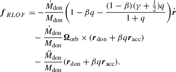
7.3. Conservation of angular momentum
Here, we investigate the evolution of the orbital AM momentum predicted by the different MT frameworks and perform a test of the consistency between the numerical and analytical expectations. For this comparison, we use the different models presented in Fig. 7. In the top panel of Fig. 11 we present the orbital AM evolution predicted by the GeMT (red and blue lines), the δ-function (black line) and emt (gray line) models. Specifically, the red line corresponds to the synchronous donor case (fdon = 1; blue line in Fig. 7), and the blue line to the evolution of the system assuming point masses (labeled PM), which neglects reaction-force contributions to the orbital evolution. In the bottom panel of Fig. 11, we compare the rate of change of the orbital AM during conservative MT with the analytical expectations.
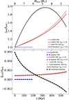 |
Fig. 11. Evolution of the orbital angular momentum (top) and its change rate (bottom) for the examples presented in Fig. 7. The blue and red lines correspond to the GeMT model for point masses and extended bodies, respectively. The black and gray lines correspond to the δ-function and emt models, respectively. The solid lines illustrate the numerical solutions, and the squares show the analytical expectations. |
We start our discussion of the orbital AM evolution with the δ-function model. Contrary to the other models, the δ-function model has been derived mathematically under the assumption of conservation of the orbital AM (Sepinsky et al. 2007b). Yet, in the limit of conservative MT, orbital AM is not conserved, as shown by the black line in the top panel of Fig. 11. The evolution of the orbital AM predicted by the δ-function model can be described analytically. Regardless of whether point masses are assumed, using Eqs. (29), (39), and (40) from Sepinsky et al. (2007b) it follows that
![Mathematical equation: $$ \begin{aligned} \frac{\langle \dot{J}_{\rm orb} \rangle }{J_{\rm orb}} = \frac{\dot{M}_{\rm 0}}{M_{1}} (1-q) \Biggl [ 1+ \frac{e}{\pi } \sqrt{\frac{1-e}{1+e}} - \frac{\sqrt{1-e^2}}{2 \pi } \Biggr ], \end{aligned} $$](/articles/aa/full_html/2026/02/aa55096-25/aa55096-25-eq70.gif) (39)
(39)
where Ṁ0 is the instantaneous MT rate and M1 is the mass of the donor (i.e., equivalent to Mdon in our notation). In the above derivation, the term ⟨Ṁ1⟩ has been replaced directly by Ṁ0. Equation (42) is shown in the bottom panel of Fig. 11 (black squares) verifying our numerical calculations.
We conclude that in the current implementation of the δ-function model, AM is not conserved in the limit of conservative MT (regardless of whether point masses are assumed), as shown in Fig. 11. Consequently, the results of studies using the δ-function model should be interpreted with caution when it comes to treatment of orbital AM. In Appendix D we provide a detailed discussion about the δ-function model and how to apply it such that orbital AM is conserved in the limit of conservative MT.
The GeMT and emt models can be used either assuming point masses or extended bodies. In the limit of point masses and conservative MT (β = 1) the models are equivalent, thus the blue line in Fig. 11 corresponds to both models, and the orbital AM is conserved, as expected (blue line in the top panel of Fig. 11). In addition, the numerical results are in very good agreement with the analytical predictions ( ; Eq. (16) overlaid in square markers in the bottom panel of Fig. 11) verifying the robustness of the models.
When accounting for extended bodies (e.g., red and gray lines in Fig. 11), reaction forces drive the secular evolution of the orbital AM; in this specific setup, it increases, and the predicted evolution differs significantly. Notably, in the point-mass approximation, the system merges at t ≈ 200 Myr, illustrating that neglecting reaction forces can significantly alter the inferred orbital evolution. Moreover, the numerical results are once again in agreement with the analytical predictions both for the GeMT and emt models. When β = 1 and rdon is given by Eq. (40) in the appendix of Hamers & Dosopoulou (2019, i.e., the low-fdon model), the orbit-averaged Eq. (16) provides also the analytical expectation for the emt model.
In general, we can thus interpret the AM evolution in the following way:
Point masses. On the one hand, the classical point-mass approximation represents a scenario where mass ejection and accretion are isotropic, making Eq. (5) well suited for studying orbital evolution due to isotropic winds but less accurate for RLOF. On the other hand, if the AM stored in the rotation of the two stars is negligible compared to the orbital AM, then point masses are valid assumptions. Fig. 11 demonstrates that the predictions of the GeMT model are robust in the point-mass limit, confirming that the examples in Fig. 9 capture both the qualitative and quantitative impact of RLOF on the orbital evolution.
Extended bodies. In Sect. 3 we demonstrated that under fully conservative MT (β = 1) the total mass is conserved, yet the orbital AM can still evolve when ejection from the donor and accretion onto the companion are anisotropic (Eq. (16)). During RLOF, the donor star loses mass anisotropically via the L1 point. The accretor also gains mass anisotropically in the case of direct accretion, while the situation becomes more complex when an accretion disk is involved. Nevertheless, if MT is conservative, the total AM must also be conserved, so any orbital gain or loss must be balanced by corresponding changes in the spin AM of the stars. In our setup (and for the emt model), the reaction force on the donor always increases the orbital AM (Eq. (16); we note that Ṁdon < 0 ), whereas the reaction force on the accretor can either increase ( ) or decrease it (
 ).
).
The extent of orbital AM that can be gained is limited by the spin AM reservoir of the donor, while the amount that can be absorbed is constrained by the critical rotational velocity of the accretor (e.g., Packet 1981) and its response to accretion (e.g., Lau et al. 2024). Fig. 11 shows that in this simplified example, the orbital AM has increased by ∼80% (red line), which is not physically expected. Therefore, the evolution presented in Fig. 7 should be interpreted qualitatively, as a self-consistent treatment of the total AM requires modeling the spin evolution of both stars. Nevertheless, Fig. 7 highlights qualitatively the impact of the donor spin fdon on the orbital evolution. Observations of systems shortly after MT with slowly spinning donors and rapidly rotating companions (e.g., Pauli et al. 2022; Müller-Horn et al. 2025) support the relevance of this mechanism.
In summary, Eqs. (40) and (41) (point-mass limit) are appropriate for studying the secular evolution of mass-transferring systems (in the limit of conservative MT, β = 1) assuming that the AM stored in the rotation of the two stars is negligible. If this assumption does not hold, however, it is necessary to account for anisotropic mass ejection and accretion, and Eqs. (29) and (30) must be adopted. A fully self-consistent treatment requires modeling the spin evolution of both stars, and enforcing conservation of the total AM, and coupling the GeMT model to detailed stellar evolution, which lies beyond the scope of this work. Nevertheless, the GeMT framework presented here captures the qualitative impact of the reaction forces on orbital AM, making its integration with binary evolution codes an important future direction.
7.4. Stability of mass transfer
RLOF in a binary system leads to either stable or unstable MT, shaping its future evolution and the properties of the final remnants. Unstable MT followed by a common-envelope (CE) phase typically results in a close binary or a merged object (e.g. Paczynski 1976), while stable MT tends to produce wider binaries (e.g. Soberman et al. 1997). The stability of the MT process and its outcomes depend mainly on two factors:4 (1) how the donor’s radius responds to mass loss and (2) how the orbit – and consequently the Roche lobe – responds to MT. Several observed systems contradict the standard understanding of MT stability. This includes systems that appear to have experienced MT from donors on the RGB (Case B) or asymptotic giant branch (AGB; Case C), yet have relatively wide orbits (Eggleton & Tout 1989), despite classical results predicting otherwise.
Numerous studies have investigated the stability of MT, suggesting that it is often severely underestimated (Woods et al. 2012; Passy et al. 2012; Pavlovskii & Ivanova 2015; Ge et al. 2010, 2015, 2020; Klencki et al. 2021; Temmink et al. 2023). In these studies, there has been great effort to model more accurately the response of the donor to mass loss, however the response of the orbit is still modeled under classical assumptions. Traditionally, the orbital response is modeled within the classical RLOF framework, assuming circular orbits and point masses. The GeMT framework improves upon these limitations in two key ways: (1) It relaxes the point-mass approximation and allows for anisotropic mass ejection and accretion, and it thereby accounts for the offset location of the L1 point. (2) It does not impose instantaneous circularization, which enables a self-consistent modeling of the orbital evolution in eccentric systems.
The deviation from the classical RLOF picture has significant implications for MT stability criteria. For instance, by relaxing the point-mass approximation, the GeMT model predicts values up to qtrans, a ≈ 1.53 for circular orbits with synchronously rotating binary components. Consequently, the critical mass ratio separating stable from unstable MT needs to increase. In summary, implementing the GeMT model in studies of mass-transferring systems using detailed evolution codes (e.g., Davis et al. 2014; Picco et al. 2026) can provide a direct comparison to observations of interacting and post-interaction binaries and help constrain binary physics.
7.5. Observed post-interaction wide binaries
Recently, it has become clear that eccentric orbits are common in wide post-interaction binary systems (see e.g., Shahaf et al. 2024). Observations reveal a notable trend: the range of eccentricities increases with orbital period (see Shahaf et al. 2024, Fig. 8), with the maximum observed eccentricities also rising as the orbital period grows. This pattern is not confined to a specific population of binaries, but is evident across diverse post-interaction systems, including long-period sdB binaries (Vos et al. 2015, 2017, 2020; Molina et al. 2022, and references therein), Barium stars (Jorissen et al. 1998; Izzard et al. 2010; Jorissen et al. 2019; Oomen et al. 2018; Escorza et al. 2019), blue stragglers (Geller & Mathieu 2011; Mathieu & Geller 2009), CH and CEMP stars (Jorissen et al. 2016; Oomen et al. 2018; Hansen et al. 2019). Despite their prevalence, the formation of these systems remains a challenge for existing models, as neither their long periods nor their high eccentricities can be reproduced by theoretical models. While several eccentricity-pumping mechanisms have been proposed, synthetic models still struggle to reproduce the general orbital properties of post-interaction binaries. Specifically:
-
The tidally enhanced wind mass-loss mechanism (Soker 2000; Bonačić Marinović et al. 2008) can generate eccentric He-WD binaries but not sdB systems, as extreme mass loss prevents helium ignition (Vos et al. 2015).
-
Circumbinary (CB) disk interactions tend to produce high eccentricities at shorter periods, contradicting observations (Dermine et al. 2013; Vos et al. 2015; Deca et al. 2018). Additionally, Oomen et al. (2020) demonstrated that binary interactions with a CB disk cannot account for the observed eccentric orbits in post-AGB binaries.
-
White dwarf kicks (e.g., Izzard et al. 2010; Chawla et al. 2025) could increase eccentricity; however, the kick mechanism remains unclear, and it is not relevant for sdB binaries.
-
Mergers in triples (Perets & Fabrycky 2009) and dynamical interactions with a tertiary companion (Toonen et al. 2020) can lead to the formation of eccentric binaries. In the first scenario, the surviving binary originates from the former outer orbit, with the merger product and the original tertiary companion as its components. In the second scenario, the Lidov-Kozai mechanism drives eccentricity growth in the inner binary. It is unlikely that triple interactions alone can account for all the eccentric orbits observed across the entire population of post-interaction binaries, however.
The long orbital periods observed (Porb ≳ 102 days) rule out a CE phase for these systems, as it would have resulted in much tighter orbits. Instead, stable MT appears to be the more plausible interaction mechanism. Classical circularization theory does not predict eccentric post-RGB and post-AGB binaries from stable RLOF, however (see Fig. 9). In summary, no proposed mechanism to date can fully explain the observed correlation between longer orbital periods and higher eccentricities, a trend that appears to hold across the entire post-interaction binary population.
At the onset of RLOF, some systems may have sufficiently low eccentricities to be classified observationally as circular binaries (Phinney 1992; Cohen et al. 2024). Isolating the effects of MT via RLOF from other physical processes, the GeMT framework, which accounts for MT in eccentric orbits, demonstrates that partial RLOF can amplify small undetectable eccentricities to measurable levels while simultaneously widening the orbit, see Fig. 9. For instance, in Fig. 12, we illustrate how the late Case B MT example presented in Fig. 9 evolves on the Porb − e plane. This evolutionary path is consistent with observed systems. We note that other physical processes, such as tides, stellar evolution, or the response of the donor and accretor to mass loss and accretion, will affect our results. Nevertheless, the GeMT model predicts a type of evolution that is relevant to all post-interaction observed systems, since it naturally predicts higher eccentricities at longer orbital periods, aligning well with numerous observed systems (see Vos et al. 2017; Jorissen et al. 2019; Kawahara et al. 2018; Molina et al. 2022; Escorza & De Rosa 2023; Yamaguchi et al. 2024, and references therein).
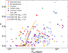 |
Fig. 12. Evolution of the system presented in Fig. 7 in the Porb − e plane. The orange, blue, and red lines correspond to the GeMT model for subsynchronous (fdon = 0.0), synchronous (fdon = 1.0), and supersynchronous donors (fdon = 2.0), respectively. The small circles and crosses indicate the initial and final positions of the systems, respectively. The red circles represent the post-AGB stars (Oomen et al. 2018). The blue triangles represent the Ba dwarfs and giants (Jorissen et al. 2019; Escorza et al. 2019, 2020), orange squares show CH subgiants (Escorza et al. 2019, 2020), green pentagons show CEMP-s stars (Hansen et al. 2016; Jorissen et al. 2016; Sperauskas et al. 2016), purple diamonds show extrinsic S stars (Fekel et al. 2000; Jorissen et al. 2019; Escorza et al. 2020), and pink plusses show wide sdB binaries (Deca et al. 2012; Barlow et al. 2012; Vos et al. 2012, 2013, 2017; Vos et al. 2019; Dorsch et al. 2021; Molina et al. 2022). |
We note, that while partial-RLOF can act as an eccentricity-pumping mechanism, the formation of wide and eccentric binaries is challenging using the δ-function model of Sepinsky et al. (2007b), except in cases where the systems start wide and eccentric at the onset of RLOF. For systems with initially low eccentricities or these that might circularize during RLOF (e → 0), the δ-function model is invalid, and the transition to the classical point-mass RLOF model cannot reproduce the formation of such systems.
Lastly, a discrepancy exists between the observed period distribution of double white dwarf (DWD) binaries and predictions from synthetic models of systems formed via stable MT. Specifically, theoretical models fail to reproduce the longest orbital periods observed in DWD binaries (see Korol et al. 2022, Fig. 11). The GeMT-model natural tendency to predict stronger orbital widening (see Fig. 9) suggests that it may help resolve this discrepancy.
8. Conclusions
We presented the general mass-transfer (GEMT) model, which is a comprehensive semianalytic framework for the orbital evolution of mass-transferring binaries. For the first time, an eccentric mass-transfer model applies to conservative and nonconservative mass transfer across the full range of eccentricities while also accounting for the spin of the donor. Our main conclusions are given below.
-
We demonstrated that for anisotropic mass ejection and accretion, such as mass transfer via RLOF, reaction forces on the donor and accretor affect the orbital evolution even in the limit of conservative mass transfer. In detailed stellar evolution studies where the component spins and angular momentum can be modeled, these additional perturbations must therefore be included when the orbital evolution driven by mass transfer is investigated.
-
For the position of the ejection point (the L1 Lagrangian point) relative to the donor, previous prescriptions introduced by Hamers & Dosopoulou (2019) were limited to cases of either massive donors (q ≫ 1) or static donors (fdon = 0.0). We introduced an accurate prescription (the most accurate to date) for the position of the Lagrangian L1 point (global-L1 model) that is applicable for any e ∈ [0.0, 0.99], q ∈ [0.1, 10.1], and fdon ∈ [0.0, 2.0]. We finally introduced a novel mass-accretion scenario in which the ejected mass follows a curved trajectory due to its initial velocity and lands on the far side of the accretor from the donor.
-
The classical RLOF framework typically assumes circularization at the onset of RLOF. In contrast, the GeMT model does not impose this assumption and instead predicts that due to phase-dependent RLOF, the orbital eccentricity can either increase or decrease. Mass-transferring binaries with up to q = Mdon/Macc ≤ 1.0 naturally evolve toward wider and more eccentric orbits, in contrast to classical expectations (Fig. 9).
-
When extended bodies are accounted for, the parameter space for orbital widening and eccentricity pumping increases (Figs. 4, 5, 6). For circular orbits, the transitional mass ratio, qtrans, a, which separates orbital widening from shrinkage, can increase from qtrans, a = 1 to qtrans, a ∼ 1.5. This implies that the critical mass ratio distinguishing stable from unstable mass transfer is systematically underestimated, regardless of the evolutionary phase of the donor. Detailed stellar evolution is necessary to quantitatively test the contribution of binary components angular momentum to the evolution of the orbital angular momentum.
-
The GeMT model predicts qualitatively and quantitatively distinct evolutionary pathways for circular and eccentric orbits. Nonetheless, we showed that in the limit of nonrotating donors (fdon = 0) and conservative mass transfer, GeMT reproduces the predictions of the emt model (Hamers & Dosopoulou 2019). Compared to the δ-function formalism (Sepinsky et al. 2007b), GeMT (point masses or extended bodies) yields a broader parameter space for eccentricity pumping and a stronger evolution of the semimajor axis and eccentricity for circular and eccentric orbits. Since the δ-function model (Sepinsky et al. 2007b) as applied in the literature does not conserve orbital angular momentum in the limit of conservative mass transfer (point mass or extended bodies), its predicted orbital evolution should be interpreted with caution (Sect. 7.3). We showed that in the limit of MT at periastron, the functional shape of the mass-transfer rate predicted by the GeMT model is a δ function, and orbital angular momentum is conserved (Appendix D). Moreover, in this limit and for point masses, the GeMT model is equivalent to the normalized δ-function model (i.e., Eqs. (D.4) and (D.5)), which verifies that the latter is also a subset of the GeMT model.
-
We demonstrated that phase-dependent RLOF can act as an eccentricity-pumping mechanism. By isolating the effects of mass transfer via RLOF from other physical processes, we showed that stable mass transfer can produce post-RLOF systems with wide and eccentric orbits. Importantly, we proved that the observed correlation of higher eccentricities and longer orbital periods naturally arises from our model. The predicted orbital evolution closely agrees with the observed properties of wide, eccentric systems containing blue stragglers (Geller & Mathieu 2011; Mathieu & Geller 2009), sdB stars (Vos et al. 2015, 2017, 2020; Molina et al. 2022), Ba stars (Jorissen et al. 1998; Izzard et al. 2010; Jorissen et al. 2019; Oomen et al. 2018; Escorza et al. 2019), CH and CEMP stars (Jorissen et al. 2016; Oomen et al. 2018; Hansen et al. 2019), and WDs (Kawahara et al. 2018; Shahaf et al. 2024; Yamaguchi et al. 2024) (see Fig. 12). Our model supports the interpretation that stable mass transfer in eccentric orbits is also relevant for other post-interaction systems with similar orbital characteristics.
Our model can be integrated into detailed and rapid stellar evolution codes to consistently treat conservative and nonconservative mass transfer in circular and eccentric orbits.
Data availability
The data necessary to reproduce Figs. 7–11 is available on Zenodo. The GeMT code will be shared upon reasonable request to the authors.
Acknowledgments
The authors would like to thank Caspar Bruenech, Floris Kummer, Martin Heemskerk, Ed van den Heuvel, Onno Pols, George Voyatzis, and Thomas Tauris for the useful discussions. The authors would like to thank Glenn-Michael Oomen for providing the observational data for Fig. 12. AP & ST acknowledges support from the Netherlands Research Council NWO (VIDI 203.061 grant). FD acknowledges support from the UK’s Science and Technology Facilities Council Grant No. ST/V005618/1. EL acknowledges support through a start-up grant from the Internal Funds KU Leuven (STG/24/073) and through a Veni grant (VI.Veni.232.205) from the Netherlands Organization for Scientific Research (NWO). This work used the following software packages: Matplotlib (Hunter 2007), Seaborn (Waskom 2021), NumPy (Harris et al. 2020), SciPy (Virtanen et al. 2020) and SymPy (Meurer et al. 2017).
References
- Barlow, B. N., Wade, R. A., Liss, S. E., Østensen, R. H., & Van Winckel, H. 2012, ApJ, 758, 58 [NASA ADS] [CrossRef] [Google Scholar]
- Belczynski, K., Kalogera, V., Rasio, F. A., et al. 2008, ApJS, 174, 223 [Google Scholar]
- Bobrick, A., Davies, M. B., & Church, R. P. 2017, MNRAS, 467, 3556 [NASA ADS] [CrossRef] [Google Scholar]
- Bonačić Marinović, A. A., Glebbeek, E., & Pols, O. R. 2008, A&A, 480, 797 [NASA ADS] [CrossRef] [EDP Sciences] [Google Scholar]
- Chawla, C., Chatterjee, S., & Breivik, K. 2025, arXiv e-prints [arXiv:2508.21805] [Google Scholar]
- Church, R. P., Dischler, J., Davies, M. B., et al. 2009, MNRAS, 395, 1127 [Google Scholar]
- Cohen, Y., Ginzburg, S., Levy, M., Bar Shalom, T., & Siman Tov, Y. 2024, MNRAS, 534, 455 [Google Scholar]
- Davis, P. J., Siess, L., & Deschamps, R. 2014, A&A, 570, A25 [NASA ADS] [CrossRef] [EDP Sciences] [Google Scholar]
- Deca, J., Marsh, T. R., Østensen, R. H., et al. 2012, MNRAS, 421, 2798 [Google Scholar]
- Deca, J., Vos, J., Németh, P., et al. 2018, MNRAS, 474, 433 [Google Scholar]
- Dermine, T., Izzard, R. G., Jorissen, A., & Van Winckel, H. 2013, A&A, 551, A50 [NASA ADS] [CrossRef] [EDP Sciences] [Google Scholar]
- Dorsch, M., Jeffery, C. S., Irrgang, A., Woolf, V., & Heber, U. 2021, A&A, 653, A120 [NASA ADS] [CrossRef] [EDP Sciences] [Google Scholar]
- Dosopoulou, F., & Kalogera, V. 2016a, ApJ, 825, 70 [NASA ADS] [CrossRef] [Google Scholar]
- Dosopoulou, F., & Kalogera, V. 2016b, ApJ, 825, 71 [NASA ADS] [CrossRef] [Google Scholar]
- Dosopoulou, F., Naoz, S., & Kalogera, V. 2017, ApJ, 844, 12 [CrossRef] [Google Scholar]
- Edwards, D. A., & Pringle, J. E. 1987, MNRAS, 229, 383 [NASA ADS] [CrossRef] [Google Scholar]
- Eggleton, P. P. 1983, ApJ, 268, 368 [Google Scholar]
- Eggleton, P. P., & Tout, C. A. 1989, Space Sci. Rev., 50, 165 [NASA ADS] [CrossRef] [Google Scholar]
- Eldridge, J. J. 2009, MNRAS, 400, L20 [NASA ADS] [CrossRef] [Google Scholar]
- Escorza, A., & De Rosa, R. J. 2023, A&A, 671, A97 [NASA ADS] [CrossRef] [EDP Sciences] [Google Scholar]
- Escorza, A., Karinkuzhi, D., Jorissen, A., et al. 2019, A&A, 626, A128 [NASA ADS] [CrossRef] [EDP Sciences] [Google Scholar]
- Escorza, A., Siess, L., Van Winckel, H., & Jorissen, A. 2020, A&A, 639, A24 [NASA ADS] [CrossRef] [EDP Sciences] [Google Scholar]
- Fekel, F. C., Joyce, R. R., Hinkle, K. H., & Skrutskie, M. F. 2000, AJ, 119, 1375 [NASA ADS] [CrossRef] [Google Scholar]
- Ge, H., Hjellming, M. S., Webbink, R. F., Chen, X., & Han, Z. 2010, ApJ, 717, 724 [NASA ADS] [CrossRef] [Google Scholar]
- Ge, H., Webbink, R. F., Chen, X., & Han, Z. 2015, ApJ, 812, 40 [Google Scholar]
- Ge, H., Webbink, R. F., Chen, X., & Han, Z. 2020, ApJ, 899, 132 [NASA ADS] [CrossRef] [Google Scholar]
- Geller, A. M., & Mathieu, R. D. 2011, Nature, 478, 356 [NASA ADS] [CrossRef] [Google Scholar]
- Hadjidemetriou, J. D. 1963, Icarus, 2, 440 [NASA ADS] [CrossRef] [Google Scholar]
- Hadjidemetriou, J. D. 1969, Ap&SS, 3, 31 [Google Scholar]
- Hamers, A. S., & Dosopoulou, F. 2019, ApJ, 872, 119 [NASA ADS] [CrossRef] [Google Scholar]
- Hamers, A. S., Rantala, A., Neunteufel, P., Preece, H., & Vynatheya, P. 2021, MNRAS, 502, 4479 [NASA ADS] [CrossRef] [Google Scholar]
- Han, Z., Podsiadlowski, P., Maxted, P. F. L., Marsh, T. R., & Ivanova, N. 2002, MNRAS, 336, 449 [Google Scholar]
- Han, Z., Podsiadlowski, P., Maxted, P. F. L., & Marsh, T. R. 2003, MNRAS, 341, 669 [NASA ADS] [CrossRef] [Google Scholar]
- Hansen, T. T., Andersen, J., Nordström, B., et al. 2016, A&A, 588, A3 [NASA ADS] [CrossRef] [EDP Sciences] [Google Scholar]
- Hansen, C. J., Hansen, T. T., Koch, A., et al. 2019, A&A, 623, A128 [NASA ADS] [CrossRef] [EDP Sciences] [Google Scholar]
- Harris, C. R., Millman, K. J., van der Walt, S. J., et al. 2020, Nature, 585, 357 [NASA ADS] [CrossRef] [Google Scholar]
- Heber, U. 2009, ARA&A, 47, 211 [Google Scholar]
- Hendriks, D. D., & Izzard, R. G. 2023, MNRAS, 524, 4315 [NASA ADS] [CrossRef] [Google Scholar]
- Hunter, J. D. 2007, Comput. Sci. Eng., 9, 90 [NASA ADS] [CrossRef] [Google Scholar]
- Hurley, J. R., Tout, C. A., & Pols, O. R. 2002, MNRAS, 329, 897 [Google Scholar]
- Izzard, R. G., Dermine, T., & Church, R. P. 2010, A&A, 523, A10 [NASA ADS] [CrossRef] [EDP Sciences] [Google Scholar]
- Jorissen, A., Van Eck, S., Mayor, M., & Udry, S. 1998, A&A, 332, 877 [NASA ADS] [Google Scholar]
- Jorissen, A., Van Eck, S., Van Winckel, H., et al. 2016, A&A, 586, A158 [NASA ADS] [CrossRef] [EDP Sciences] [Google Scholar]
- Jorissen, A., Boffin, H. M. J., Karinkuzhi, D., et al. 2019, A&A, 626, A127 [NASA ADS] [CrossRef] [EDP Sciences] [Google Scholar]
- Kashi, A., & Soker, N. 2018, MNRAS, 480, 3195 [NASA ADS] [Google Scholar]
- Kawahara, H., Masuda, K., MacLeod, M., et al. 2018, AJ, 155, 144 [Google Scholar]
- Klencki, J., Nelemans, G., Istrate, A. G., & Chruslinska, M. 2021, A&A, 645, A54 [EDP Sciences] [Google Scholar]
- Korol, V., Belokurov, V., & Toonen, S. 2022, MNRAS, 515, 1228 [NASA ADS] [CrossRef] [Google Scholar]
- Lajoie, C.-P., & Sills, A. 2011, ApJ, 726, 67 [Google Scholar]
- Lau, M. Y. M., Hirai, R., Mandel, I., & Tout, C. A. 2024, ApJ, 966, L7 [NASA ADS] [CrossRef] [Google Scholar]
- Li, Z., Chen, X., Chen, H.-L., & Han, Z. 2019, ApJ, 871, 148 [NASA ADS] [CrossRef] [Google Scholar]
- Li, Z., Chen, X., Chen, H.-L., et al. 2020, ApJ, 893, 2 [NASA ADS] [CrossRef] [Google Scholar]
- Limber, D. N. 1963, ApJ, 138, 1112 [Google Scholar]
- Lubow, S. H., & Shu, F. H. 1975, ApJ, 198, 383 [NASA ADS] [CrossRef] [Google Scholar]
- Luk’yanov, L. G. 2008, Astron. Rep., 52, 680 [Google Scholar]
- Marchant, P., Pappas, K. M. W., Gallegos-Garcia, M., et al. 2021, A&A, 650, A107 [NASA ADS] [CrossRef] [EDP Sciences] [Google Scholar]
- Mathieu, R. D., & Geller, A. M. 2009, Nature, 462, 1032 [NASA ADS] [CrossRef] [Google Scholar]
- Meurer, A., Smith, C. P., Paprocki, M., et al. 2017, PeerJ Comput. Sci., 3, e103 [CrossRef] [Google Scholar]
- Moe, M., & Di Stefano, R. 2017, ApJS, 230, 15 [Google Scholar]
- Molina, F., Vos, J., Németh, P., et al. 2022, A&A, 658, A122 [NASA ADS] [CrossRef] [EDP Sciences] [Google Scholar]
- Müller-Horn, J., El-Badry, K., Rix, H.-W., et al. 2025, A&A, 701, A9 [NASA ADS] [CrossRef] [EDP Sciences] [Google Scholar]
- Oomen, G.-M., Van Winckel, H., Pols, O., et al. 2018, A&A, 620, A85 [NASA ADS] [CrossRef] [EDP Sciences] [Google Scholar]
- Oomen, G.-M., Pols, O., Van Winckel, H., & Nelemans, G. 2020, A&A, 642, A234 [NASA ADS] [CrossRef] [EDP Sciences] [Google Scholar]
- Packet, W. 1981, A&A, 102, 17 [NASA ADS] [Google Scholar]
- Paczynski, B. 1976, IAU Symp., 73, 75 [NASA ADS] [Google Scholar]
- Paczyński, B., & Sienkiewicz, R. 1972, Acta Astron., 22, 73 [NASA ADS] [Google Scholar]
- Parkosidis, A., Toonen, S., Laplace, E., & Dosopoulou, F. 2025, arXiv e-prints [arXiv:2511.07190] [Google Scholar]
- Passy, J.-C., Herwig, F., & Paxton, B. 2012, ApJ, 760, 90 [NASA ADS] [CrossRef] [Google Scholar]
- Pauli, D., Oskinova, L. M., Hamann, W. R., et al. 2022, A&A, 659, A9 [NASA ADS] [CrossRef] [EDP Sciences] [Google Scholar]
- Pavlovskii, K., & Ivanova, N. 2015, MNRAS, 449, 4415 [Google Scholar]
- Perets, H. B., & Fabrycky, D. C. 2009, ApJ, 697, 1048 [Google Scholar]
- Petrova, A. V., & Orlov, V. V. 1999, AJ, 117, 587 [Google Scholar]
- Phinney, E. S. 1992, Philos. Trans. R. Soc. Lond. Ser. A, 341, 39 [NASA ADS] [Google Scholar]
- Picco, A., Marchant, P., Sana, H., & Nelemans, G. 2024, A&A, 681, A31 [NASA ADS] [CrossRef] [EDP Sciences] [Google Scholar]
- Picco, A., Marchant, P., Sana, H., et al. 2026, A&A, 705, A225 [NASA ADS] [CrossRef] [EDP Sciences] [Google Scholar]
- Podsiadlowski, P., Han, Z., Lynas-Gray, A. E., & Brown, D. 2008, ASP Conf. Ser., 392, 15 [NASA ADS] [Google Scholar]
- Pols, O. R., Karakas, A. I., Lattanzio, J. C., & Tout, C. A. 2003, ASP Conf. Ser., 303, 290 [NASA ADS] [Google Scholar]
- Portegies Zwart, S. F., & Verbunt, F. 1996, A&A, 309, 179 [NASA ADS] [Google Scholar]
- Postnov, K. A., & Yungelson, L. R. 2014, Liv. Rev. Relat., 17, 3 [NASA ADS] [CrossRef] [Google Scholar]
- Preece, H. P., Hamers, A. S., Neunteufel, P. G., Schaefer, A. L., & Tout, C. A. 2022, ApJ, 933, 25 [NASA ADS] [CrossRef] [Google Scholar]
- Pringle, J. E., & Wade, R. A. 1985, Interacting Binary Stars (Cambridge University Press) [Google Scholar]
- Raguzova, N. V., & Popov, S. B. 2005, Astron. Astrophys. Trans., 24, 151 [Google Scholar]
- Regös, E., Bailey, V. C., & Mardling, R. 2005, MNRAS, 358, 544 [Google Scholar]
- Rocha, K. A., Hur, R., Kalogera, V., et al. 2025, ApJ, 983, 39 [Google Scholar]
- Sana, H., de Mink, S. E., de Koter, A., et al. 2012, Science, 337, 444 [Google Scholar]
- Sciarini, L., Ekström, S., Eggenberger, P., et al. 2024, A&A, 681, L1 [NASA ADS] [CrossRef] [EDP Sciences] [Google Scholar]
- Sepinsky, J. F., Willems, B., & Kalogera, V. 2007a, ApJ, 660, 1624 [NASA ADS] [CrossRef] [Google Scholar]
- Sepinsky, J. F., Willems, B., Kalogera, V., & Rasio, F. A. 2007b, ApJ, 667, 1170 [NASA ADS] [CrossRef] [Google Scholar]
- Sepinsky, J. F., Willems, B., Kalogera, V., & Rasio, F. A. 2009, ApJ, 702, 1387 [NASA ADS] [CrossRef] [Google Scholar]
- Sepinsky, J. F., Willems, B., Kalogera, V., & Rasio, F. A. 2010, ApJ, 724, 546 [NASA ADS] [CrossRef] [Google Scholar]
- Shahaf, S., Hallakoun, N., Mazeh, T., et al. 2024, MNRAS, 529, 3729 [NASA ADS] [CrossRef] [Google Scholar]
- Smith, T., & Kaplinghat, M. 2025, AAS Meet. Abstr., 245, 419.04 [Google Scholar]
- Soberman, G. E., Phinney, E. S., & van den Heuvel, E. P. J. 1997, A&A, 327, 620 [NASA ADS] [Google Scholar]
- Soker, N. 2000, A&A, 357, 557 [NASA ADS] [Google Scholar]
- Sperauskas, J., Začs, L., Schuster, W. J., & Deveikis, V. 2016, ApJ, 826, 85 [NASA ADS] [CrossRef] [Google Scholar]
- Temmink, K. D., Pols, O. R., Justham, S., Istrate, A. G., & Toonen, S. 2023, A&A, 669, A45 [NASA ADS] [CrossRef] [EDP Sciences] [Google Scholar]
- Toonen, S., Nelemans, G., & Portegies Zwart, S. 2012, A&A, 546, A70 [NASA ADS] [CrossRef] [EDP Sciences] [Google Scholar]
- Toonen, S., Portegies Zwart, S., Hamers, A. S., & Bandopadhyay, D. 2020, A&A, 640, A16 [NASA ADS] [CrossRef] [EDP Sciences] [Google Scholar]
- van den Heuvel, E. P. J., Portegies Zwart, S. F., & de Mink, S. E. 2017, MNRAS, 471, 4256 [Google Scholar]
- van der Helm, E., Portegies Zwart, S., & Pols, O. 2016, MNRAS, 455, 462 [Google Scholar]
- Virtanen, P., Gommers, R., Oliphant, T. E., et al. 2020, Nat. Methods, 17, 261 [Google Scholar]
- Vos, J., Østensen, R. H., Degroote, P., et al. 2012, A&A, 548, A6 [NASA ADS] [CrossRef] [EDP Sciences] [Google Scholar]
- Vos, J., Østensen, R. H., Németh, P., et al. 2013, A&A, 559, A54 [NASA ADS] [CrossRef] [EDP Sciences] [Google Scholar]
- Vos, J., Østensen, R. H., Marchant, P., & Van Winckel, H. 2015, A&A, 579, A49 [NASA ADS] [CrossRef] [EDP Sciences] [Google Scholar]
- Vos, J., Østensen, R. H., Vučković, M., & Van Winckel, H. 2017, A&A, 605, A109 [NASA ADS] [CrossRef] [EDP Sciences] [Google Scholar]
- Vos, J., Vučković, M., Chen, X., et al. 2019, MNRAS, 482, 4592 [NASA ADS] [CrossRef] [Google Scholar]
- Vos, J., Bobrick, A., & Vučković, M. 2020, A&A, 641, A163 [NASA ADS] [CrossRef] [EDP Sciences] [Google Scholar]
- Waskom, M. L. 2021, J. Open Source Softw., 6, 3021 [CrossRef] [Google Scholar]
- Woods, T. E., Ivanova, N., van der Sluys, M. V., & Chaichenets, S. 2012, ApJ, 744, 12 [NASA ADS] [CrossRef] [Google Scholar]
- Yamaguchi, N., El-Badry, K., Fuller, J., et al. 2024, MNRAS, 527, 11719 [Google Scholar]
Traditionally, β is defined as the fraction of mass transferred from the donor star that is ejected from the system in the vicinity of the accretor (e.g., Soberman et al. 1997). Here, we follow the notation introduced in Sect. 7.2, pages 9–12, of lecture notes on binary star evolution by Onno Pols.
Perturbations arising from other physical processes, such as gravitational waves, can remove orbital AM without mass loss from the system. Such perturbations are beyond the scope of this paper.
In a similar approach the initial semimajor axis is determined by conserving orbital AM, yielding acirc = a(1 − e2), which also ensures circular post-MT orbits.
A third factor is the accretor response to MT (Lau et al. 2024), but it is considered of secondary importance.
The regular singular point reflects a physical assumption of the model; when approaching the boundary, the instantaneous MT rate approaches zero because the stellar radius Rdon tends to become equal to the Roche lobe equivalent radius RL (see Eq. 19).
Appendix A: Parametrizing angular momentum loss
A perturbation induced on a binary system can give rise to changes in the Keplerian orbit elements. Using the true anomaly, ν, the binary separation is
 (A.1)
(A.1)
and the relative velocity is given by
 (A.2)
(A.2)
In addition, the perturbation given by Eq. (7) has the form  , where
  ,
,  and
and  . Using Eq. (A.2) we re-write the perturbation as
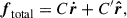 (A.3)
(A.3)
where 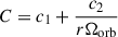 and
and 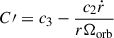 .
.
The semimajor axis and the eccentricity of the orbit change based on Eqs. (13) and (14), respectively. Under the influence of  , one derives
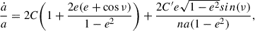 (A.4)
(A.4)
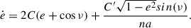 (A.5)
(A.5)
Substituting Eq. (A.5) into Eq. (A.4) and multiplying both sides by, Ma(1 − e2) we have
![Mathematical equation: $$ \begin{aligned} M(1-e^2)\dot{a} = 2C a M(1-e^2) + 2 a eM\dot{e}&\nonumber \\ a(1-e^2)\dot{M} + M(1-e^2)\dot{a} - 2 a eM\dot{e} = \nonumber \\ 2C a M(1-e^2)+ a(1-e^2)\dot{M} \nonumber \\ \frac{d}{dt} [M a (1-e^2)] = [M a (1-e^2)] \Biggl (2C +\frac{\dot{M}}{M}\Biggr )&\nonumber \\ \frac{\frac{d}{dt} [GM a (1-e^2)]}{[GM a (1-e^2)]} = \Biggl (2C +\frac{\dot{M}}{M}\Biggr )&\nonumber \\ \frac{1}{2}\frac{\frac{d}{dt} [GM a (1-e^2)]}{[GM a (1-e^2)]} = \Biggl (C +\frac{1}{2} \frac{\dot{M}}{M}\Biggr )&\nonumber \\ \frac{\dot{l}_{\rm orb}}{l_{\rm orb}} = \Biggl (C +\frac{1}{2} \frac{\dot{M}}{M}\Biggr )&\nonumber ,\\ \end{aligned} $$](/articles/aa/full_html/2026/02/aa55096-25/aa55096-25-eq86.gif) (A.6)
(A.6)
where l = J/μ the orbital AM per reduced mass. Additionally, by differentiating the orbital AM, we derive
![Mathematical equation: $$ \begin{aligned} \frac{\dot{J}_{\rm orb}}{J_{\rm orb}} + \frac{\dot{M}}{M} - \frac{\dot{M}_{\rm acc}}{M_{\rm acc}} - \frac{\dot{M}_{\rm don}}{M_{\rm don}} = \frac{1}{2} \frac{\frac{d}{dt} [GM a (1-e^2)]}{[GM a (1-e^2)]}, \end{aligned} $$](/articles/aa/full_html/2026/02/aa55096-25/aa55096-25-eq87.gif) (A.7)
(A.7)
and by substituting Eq. (A.6) into Eq. (A.7) and using Eq. (3), we find
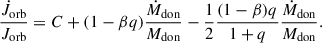 (A.8)
(A.8)
At this point, C needs to be specified. As shown by Eqs. (A.3) and (7), we define
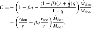 (A.9)
(A.9)
where the negative sign in front of the term associated with the accretion point corresponds to  , while the positive sign to
  . Hence, after substituting C into Eq. (A.8), we find
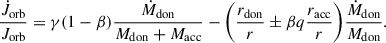 (A.10)
Appendix B: The inner Lagrangian L1 point in asynchronous and eccentric binaries
An accurate description of the location of the inner Lagrangian L1 point is essential for understanding the evolution of mass-transferring binaries via RLOF. The global-L1, XL1(fdon, q, e), determines the position of the L1 point, relative to the donor center of mass, at periapsis in units of the instantaneous distance between the two stars, given explicitly by
 (B.1)
(B.1)
Equation (B.1) achieves an accuracy better than ∼9% for 0.0 ≤ fdon ≤ 2.0, 0.1 ≤ q ≤ 10.1 and 0.0 ≤ e ≤ 0.99.
We approximate the position of L1 over a single orbit in natural units using the product XL1(fdon, q, e)r. To assess the accuracy of our prescription, we calculate the fractional error at the predicted positions, as
 (B.2)
(B.2)
where XL1(fdon, q, e, ℰ) is the numerical solution of Eq. (8) for 0.0 ≤ fdon ≤ 2.0, 0.1 ≤ q ≤ 10.1, 0.0 ≤ e ≤ 0.99 and 0.0 ≤ ℰ ≤ 2π. We have arbitrary defined the region of "good accuracy" as the part of the parameter space where the fractional error is ≤10%. Figure B.1 illustrates the fractional error at the position of the L1 point over one orbit.
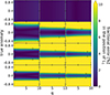 |
Fig. B.1. Fractional error of the position of the L1 point over one orbit for the global-L1 model. Top to bottom, e = 0.0, 0.3, 0.6, and 0.9. Left to right, fdon = 0.5, 1.0, and 1.5. The dashed line corresponds to a fractional error of 10%. |
In Fig. B.1 we observe that for circular orbits, the fractional error remains within ≤3% for 0.0 ≤ fdon ≤ 2.0 and 0.1 ≤ q ≤ 10.1. For eccentric orbits, the region of good accuracy becomes increasingly confined to the vicinity of periapsis as eccentricity increases. The model accuracy is largely independent of the mass ratio q, but exhibits a weak dependence on the degree of asynchronism fdon. Specifically, the region of good accuracy shrinks around periapsis for donors with progressively higher spin rates (supersynchronous rotation). We highlight that the region of "good accuracy" essentially mirrors the mass loss rate given by Eq. (28). The position of the L1 point is less accurate away from periapsis, where the mass loss rate is very low, but remains highly accurate near periapsis, where mass loss peaks. For comparison purposes, we show the same plot in Fig. B.2, for the low-fdon model.
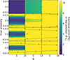 |
Fig. B.2. Fractional error of the position of the L1 point over one orbit for the low-fdon model. Top to bottom, e = 0.0, 0.3, 0.6, and 0.9. Left to right, fdon = 0.5, 1.0, and 1.5. The dashed lines correspond to fractional errors of 10% and 100%. |
The global-L1 model, XL1(fdon, q, e), is a fit to the numerical solutions of Eq. (11) over the parameter ranges 0.0 ≤ fdon ≤ 2.0, 0.1 ≤ q ≤ 10.1 and 0.0 ≤ e ≤ 0.99. An alternative fit, XL1, sep(fdon, q, e), is provided by Sepinsky et al. (2007b), see their Eq. A15). To compare the two fits, we compute the predicted positions using both XL1(fdon, q, e) and XL1, sep(fdon, q, e) and evaluate their accuracy using the root mean squared error (RMSE),
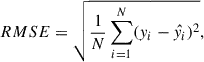 (B.3)
(B.3)
where yi represents the numerical solutions and  the predicted values from each fit. Figure B.3 illustrates the accuracy of the two fits. The global-L1 model illustrates overall a better agreement with the numerical solutions.
 |
Fig. B.3. Comparison of the accuracy of the two fits in predicting the position of the L1 point at the periapsis of the binary orbit for varying fdon, q, and e. The blue and orange colors correspond to Eq. A.15 of Sepinsky et al. (2007b) and the global-L1 model (Eq. B.1), respectively. |
Appendix C: Functions appearing in the orbit-averaged equations of motion in the limit of circular orbits
In the limit of ℰ0 → π, RLOF occurs during the whole orbit. Moreover, as the orbit circularize (e → 0), the following limits apply to the orbit-averaged equations of motion (Eqs. 29 and 30):
 (C.1)
(C.1)
assuming x ≠ 1.
Appendix D: The limit of δ-function MT rate
The GeMT and the δ−function models are two fundamentally different formalisms. The GeMT model accounts for the degree of RLOF through the parameter x (Eq. 21), which evolves self-consistently as the Roche lobe equivalent radius changes during the integration. In contrast, this parameter is absent from the secular evolution equations of the δ−function formalism (Sepinsky et al. 2007b, 2009). This is a fundamental difference between the two models. Nevertheless, the physical motivation behind the δ−function model is reflected along the border separating no from partial RLOF regions (black dashed line in Fig. D.1).
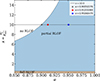 |
Fig. D.1. Zoom in region of Fig. 3 showing the parameter space of applicability of the GeMT model. The horizontal line corresponds to x = 10.0. |
In Fig. D.1 we present a small region of the e − x plane and systems for x = 10.0 and varying e. Moreover, in Fig. D.2, we present the respective normalized MT rate as a function of eccentric anomaly.
 |
Fig. D.2. Normalized mass-transfer rate as a function of eccentric anomaly. We selected ⟨Ṁdoon⟩ = 1 M⊙ yr−1 for representation purposes. |
The δ-function framework assumes that in eccentric orbits, MT occurs only at periastron, where the stellar separation is at minimum. In the GeMT formalism, this behavior naturally arises at the transition between the no RLOF and partial RLOF regimes (i.e., dashed black line in Fig D.1). Near this boundary, the functional shape of the MT rate closely resembles a δ function (gray point in D.1 and gray line in Fig. D.2) as expected when MT is strongly confined around periastron. Away from the boundary (i.e., red and blue points in Fig. D.1), however, the functional shape of the MT rate is flatter because MT occurs during a larger part of the orbit (i.e., red and blue lines in Fig. D.2).
On the boundary (i.e., cos(E0)→1, see Eq. 22), the functional shape of the MT rate approaches a δ function. In this limit, the ratios  and
and  in Eqs. (40) and (41) have a regular singular point,5 thus the true behavior of the equations is determined as
 (D.1)
(D.1)
and the secular equations of motion (Eqs. 40 and 41) become
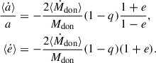 (D.2)
(D.2)
Consequently, the functional shape of the MT rate predicted by the GeMT model approaches a δ function when MT occurs only at periastron (i.e., cos(E0)→1), then the secular evolution is given by Eqs. (D.1), and (D.2).
We note that when using Eqs. (39) and (40) of Sepinsky et al. (2007b) the orbital AM is not conserved (see Fig. 11). The reason stems from the treatment of the instantaneous MT rate Ṁ0, which is assumed to be known and constant in the works of Sepinsky et al. (2007b, 2009) and it is calculated numerically in the work of Rocha et al. (2025). In the GeMT model (and in the emt model), we re-express the instantaneous MT rate Ṁdon,0 in Eqs. (25) and (26) in terms of the orbit-averaged MT rate ⟨Ṁdoon⟩, which ideally would be calculated numerically and self-consistently, as described in Sect. 4. This procedure ensures conservation of the secular orbital AM (in the point-mass limit), as shown in Fig. 11. This is expected, since secular AM conservation is obtained only when the donor and accretor masses vary in a way that is normalized to the orbit-averaged MT rate, consistent with the secular changes in a and e.
In contrast, Eq. (39) and (40) of Sepinsky et al. (2007b), and Eqs. 18 and 19 of Sepinsky et al. 2009) have been used in the literature (e.g., Sepinsky et al. 2007b, 2009; Dosopoulou & Kalogera 2016a,b; Rocha et al. 2025) without the proper normalization factor required by orbit averaging Eq. (32) of Sepinsky et al. (2007b). This is equivalent to substituting  directly with Ṁ0 during the derivation of Eq. (42), which tracks the orbital AM evolution predicted by Eqs. (39) and (40) of Sepinsky et al. (2007b), as shown in Fig. 11. This leads to a secular evolution, which although formally derived under the assumption of conserved secular orbital AM, does not actually conserve it in practice, as seen in Fig. 11.
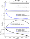 |
Fig. D.3. Secular evolution using the δ-function model. The black line shows the evolution predicted by Eqs. (39) and (40) from Sepinsky et al. (2007b), for Ṁ0 = 10−8 M⊙ yr−1. The black squares show Eq. (42). The blue line shows the evolution predicted by Eqs. (D.4), and (D.5), for |

When the same normalization procedure as used in our model is applied to the δ-function case, however, the secular orbital AM momentum is conserved. Specifically, the proper normalization can be derived by orbit averaging Eq. (32), yielding
 (D.3)
(D.3)
and finally Eqs. (39) and (40) should be written as
![Mathematical equation: $$ \begin{aligned} \langle \frac{da}{dt}\rangle _{\rm sec}&= \frac{2 \langle \dot{M}_{1} \rangle }{M_{1}} \frac{a}{(1-e)^{2}} \Biggl [qe \frac{|\boldsymbol{r}_{A_2}|}{a}\cos (\phi _P)+e\frac{|\boldsymbol{r}_{A_{1},P}|}{a} \nonumber \\&+(q-1)(1-e^2)\Biggr ], \\ \langle \frac{de}{dt}\rangle _{\rm sec}&= \frac{\langle \dot{M}_{1} \rangle }{M_{1}} \frac{1+e}{1-e} \Biggl [q \frac{|\boldsymbol{r}_{A_2}|}{a}\cos (\phi _P)+\frac{|\boldsymbol{r}_{A_{1},P}|}{a} \nonumber \\&+2(1-e)(q-1)\Biggr ]. \end{aligned} $$](/articles/aa/full_html/2026/02/aa55096-25/aa55096-25-eq105.gif) (D.4)
(D.4)
Notably, (D.4), and (D.5) have a different dependency on e than those presented by Sepinsky et al. (2007b). Using Eq. (29), (39), (40) from Sepinsky et al. (2007b), and Eqs. (D.3) it follows that
 (D.5)
(D.5)
as expected in the limit of conservative MT. Importantly, the terms related to |rA1, P| and |rA2| cancel each other out both in the derivations of Eqs. (D.6) and (42), demonstrating that in contrast to the emt and GeMT models, the orbital AM evolution predicted by the δ-function model is equivalent for point masses and extended bodies.
In Fig. D.3 we compare the secular evolution of the system introduced in Sect. 6.1 using Eqs. (39) and (40) from Sepinsky et al. (2007b) (black line; assuming Ṁ0 = 10−8 M⊙ yr−1) with our results obtained from Eqs. (D.4), and (D.5) (blue line; Ṁdon = 10−8 M⊙ yr−1).
The predicted evolution between the two sets of equations is significantly different, as expected (see Eq. D.3). In addition, the evolution shown by the blue line (Eqs. D.4, and D.5), is more similar to that predicted by the emt and GeMT models in Fig. 7. Nevertheless, we see that the normalized δ-function model can still lead to negative eccentricities similar to the δ-function model of Sepinsky et al. (2007b), as first noted by Hamers & Dosopoulou (2019), highlighting that this behavior is inherent to the model. Most importantly, though, we see that when using the normalized δ-function model, the orbital AM is conserved (blue line) in the limit of conservative MT, contrary to the case when Eqs. (39) and (40) of Sepinsky et al. (2007b), black line) are used directly. Finally, we note, that Eqs. (D.4), and (D.5) also represent the δ-function MT rate limit of our model (i.e., cos(E0)→1); they are equivalent to Eqs. (D.1), and (D.2) in the limit of point masses (i.e., |rA1, P|=|rA2| = 0) verifying that the corrected δ-function model is a subset of the GeMT model.
We conclude by mentioning the δ-function model has been implemented inconsistently in the literature. First, it has been implemented by using directly Eqs. (39) and (40) of Sepinsky et al. (2007b) (or Eqs. 18 and 19 of Sepinsky et al. 2009) without the proper required normalization factor (e.g., Sepinsky et al. 2007b, 2009; Dosopoulou & Kalogera 2016a,b; Rocha et al. 2025). This leads to a secular evolution, which although formally derived under the assumption of conserved secular orbital AM, does not actually conserve it in practice, as seen in Fig. D.3. Second, in Hamers & Dosopoulou (2019) the δ-function model was implemented by replacing Ṁ0 by 2π⟨Ṁ1⟩, which is not the proper normalization factor, and thus the orbital AM is not conserved in the limit of conservative MT in their implementation either. Here, we derive the normalized δ-function model (Eqs. D.4, and D.5), which has a different dependency on e and we verify both numerically and analytically that it conserves the orbital AM in the limit of conservative MT.
In summary, when cos(E0)→1 (i.e., MT occurs exactly at periastron), the functional shape of the MT rate predicted by the GeMT model is a δ function. In this limit, and adopting point masses, the GeMT model is equivalent to the corrected δ-function model of Sepinsky et al. (2007b), i.e., Eqs. D.4 and D.5). Nevertheless, even if the initial conditions are set to approximate this limit, the parameter x evolves over time. As a result, the secular evolution predicted by the emt and GeMT models is expected to diverge from the δ-function model as the integration proceeds, highlighting the fundamental difference between these formalisms.
Appendix E: Explicit expressions for the functions appearing in the orbit-averaged equations of motion
In this section we explicitly present the dimensionless functions  and he(e, x), as referenced in Sect. 4.
E.1. Normalization
The dimensionless normalization function obtained by orbit-averaging the mass loss rate Ṁdon given by Eq. (21),
 (E.1)
(E.1)
E.2. Dimensionless functions associated with the relative acceleration of the stars
The dimensionless functions associated with the terms in fRLOF (Eq. 7) proportional to ṙ, which are related to the distribution of the total mass in the system and the effects of mass and angular momentum loss. Furthermore, these terms appear in Eqs. (29) and (30) regardless of whether point masses or extended bodies are assumed,
 (E.2)
(E.2)
 (E.3)
(E.3)
E.3. Dimensionless functions associated with the ejection point
The dimensionless functions associated with the terms in fRLOF (Eq. 7) that are related to the ejection point. These terms appear by modeling the donor as an extended body,
![Mathematical equation: $$ \begin{aligned} g_{a}&(e,x) =\frac{1}{32 \pi } \Biggl ( ex \Bigl ( - 16(6+e^{2}(x-3) - 4x)x\sin {(\mathcal{E} _0)} \\&+ e^{2}x [16(1- x) \sin {(3 \mathcal{E} _0 )} + 3 e x \sin {(4 \nonumber \mathcal{E} _0)}] \\ \nonumber&+ 8e(((e^{2} + 2)x - 6)x + 3) \sin {(2 \mathcal{E} _0)}\Bigr ) \\ \nonumber&+ 4 \mathcal{E} _0 x(-8(3+(x-3)x)+e^{2}(12+(e^{2}-8)x^{2})) \\&+ 64 \sqrt{1 - e^{2}} {\text{ asin}}{(\frac{\sqrt{e + 1} \sqrt{\frac{1}{1 - e}} \sin {(\frac{\mathcal{E} _0}{2} )}}{\sqrt{\cos ^{2}{(\frac{\mathcal{E} _0}{2} )} + \frac{(e + 1) \sin ^{2}{(\frac{\mathcal{E} _0}{2} )}}{1 - e}}} )}\Biggr ), \\ \nonumber \end{aligned} $$](/articles/aa/full_html/2026/02/aa55096-25/aa55096-25-eq111.gif) (E.4)
(E.4)
![Mathematical equation: $$ \begin{aligned} g_{e}&(e,x) = \frac{(1 - e^{2})}{48 \pi e} \Biggl (e^{2} x \Bigl (e x [3 e x \sin {(4 \nonumber \mathcal{E} _0 )} \\ \nonumber&+ (18 - 20 x) \sin {(3 \mathcal{E} _0 )}] \\ \nonumber&+ 6([2 (e^{2} + 4)x - 15]x + 6) \sin {(2 \mathcal{E} _0 )}\Bigr ) \\ \nonumber&- 6 e \Bigl ([e^{2} x (14 x - 15) + 8\bigl ((x - 3)x + 3\bigr )]x - 4\Bigr ) \sin {(\mathcal{E} _0 )} \\ \nonumber&+ 12\Bigl (e^{2} x \bigr ([(e^{2} + 4)x - 9]x + 6 \bigl ) - 2 \Bigr ) \mathcal{E} _0 \\&+ 48 \sqrt{1 - e^{2}} {\text{ asin}}{(\frac{\sqrt{e + 1} \sqrt{\frac{1}{1 - e}} \sin {(\frac{\mathcal{E} _0}{2} )}}{\sqrt{\cos ^{2}{(\frac{\mathcal{E} _0}{2} )} + \frac{(e + 1) \sin ^{2}{(\frac{\mathcal{E} _0}{2} )}}{1 - e}}} )}\Biggr ). \\ \nonumber \end{aligned} $$](/articles/aa/full_html/2026/02/aa55096-25/aa55096-25-eq112.gif) (E.5)
(E.5)
E.4. Dimensionless functions associated with the accretion point
The dimensionless functions associated with the terms in fRLOF (Eq. 7) that are related to the accretion point. These terms appear by modeling the accretor as an extended body,
 (E.6)
(E.6)
![Mathematical equation: $$ \begin{aligned} h_{e}&(e,x) =\frac{1}{48 e\pi } \Biggl ( \frac{1}{-1+e\cos {(\mathcal{E} _0})}(-1+e^{2}) \nonumber \\&\Bigl [12 \mathcal{E} _0 (-2+e^{2}x^{2}(-3+2x)) \nonumber \\&+ 4e \Bigl (3\mathcal{E} _0(2+e^{2}(3-2x)x^{2})\cos {(\mathcal{E} _0}) +6\sin {(\mathcal{E} _0}) \nonumber \\&+x(-1+e\cos {(\mathcal{E} _0}))\Bigl (4(9+x(-9+(3+2e^{2})x)) \nonumber \\&+ ex(9(3-2x)\cos {(\mathcal{E} _0)}+4ex\cos {(2\mathcal{E} _0}))\Bigr )\sin {(\mathcal{E} _0})\Bigl )\Bigl ] \nonumber \\&+48\sqrt{1-e^2}{\text{ asin}}{(\frac{\sqrt{e + 1} \sqrt{\frac{1}{1 - e}} \sin {(\frac{\mathcal{E} _0}{2} )}}{\sqrt{\cos ^{2}{(\frac{\mathcal{E} _0}{2} )} + \frac{(e + 1) \sin ^{2}{(\frac{\mathcal{E} _0}{2} )}}{1 - e}}} )}\Biggr ). \\ \nonumber \end{aligned} $$](/articles/aa/full_html/2026/02/aa55096-25/aa55096-25-eq114.gif) (E.7)
(E.7)
All Tables
All Figures
|
Fig. 1. Position of the L1 point relative to the donor center of mass at the periapsis of the binary orbit in units of the instantaneous binary separation. The thick lines show the numerical solutions of Eq. (11). The dotted, dashed, and thin lines illustrate the high-q, low-fdon, and global-L1 models, respectively. Blue, orange, and green correspond to fdon = 0.5, 1.0, and 1.5, respectively, and e = 0.3 for all models. The low-fdon prescription is independent of fdon. |
| In the text | |
|
Fig. 2. Position of the L1 point relative to the donor center of mass in units of the semimajor axis a for q = 1 and fdon = 1 as a function of the true anomaly. The thick lines are the numerical solutions of Eq. (8). From top to bottom, the dotted, dashed, and thin lines illustrate the high-q, low-fdon, and global-L1 models, respectively. Blue, orange, green and red correspond to e = 0.0, 0.3, 0.6, and 0.9, respectively. |
| In the text | |
|
Fig. 3. Graphical representation of the mass-transfer regimes based on the mass-transfer rate formulation by Hamers & Dosopoulou (2019). The white region indicates no mass transfer, i.e. no RLOF. The light blue region corresponds to partial RLOF, where mass transfer occurs during part of the orbit. The light brown region represents full RLOF, with continuous mass transfer throughout the entire orbit. |
| In the text | |
|
Fig. 4. Secular change rate of the semimajor axis as a function of the mass ratio q and the level of synchronism fdon of the donor in the limit of circular orbits. From top to bottom, GeMT model in the limit of point masses, extended bodies for |
| In the text | |
|
Fig. 5. Secular change rate of the semimajor axis in the limit of conservative mass transfer as a function of mass ratio q and eccentricity e. From top to bottom, GeMT model in the limit of point masses, extended bodies for |
| In the text | |
|
Fig. 6. Similar to Fig. 5, but the color gradient now illustrates the secular change rate of the eccentricity. |
| In the text | |
|
Fig. 7. Evolution of the semimajor axis (top), eccentricity (middle), mass ratio q, and angle ℰ (bottom) as a function of time during mass transfer. The dashed black and gray lines correspond to the emt and δ-function (fdon = 1.0) models, respectively. The orange, blue and red lines correspond to the GeMT model, for subsynchronous (fdon = 0.0), synchronous (fdon = 1.0) and supersynchronous donors (fdon = 2.0), respectively. In the bottom panel, the two horizontal dotted lines indicate ℰ0 = π and q = 1. |
| In the text | |
|
Fig. 8. Evolution of the systems presented in Fig. 7 in the e − x plane for subsynchronous (fdon = 0.0), synchronous (fdon = 1.0), and supersynchronous donors (fdon = 2.0). The circles and triangles indicate the initial and final positions of the systems, respectively. |
| In the text | |
|
Fig. 9. Similar to Fig. 7, but now for an initially nearly circular binary (e = 0.001). The orange, blue, and red lines correspond to the GeMT model for a = 1.08, 1.11, and 1.14 au and Macc = 0.7, 0.8, and 0.9 M⊙, respectively. In the top panel, the dotted lines illustrate the classical analytic expectation that |
| In the text | |
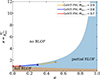 |
Fig. 10. Similar to Fig. 8, but now for the systems presented in Fig. 9. |
| In the text | |
|
Fig. 11. Evolution of the orbital angular momentum (top) and its change rate (bottom) for the examples presented in Fig. 7. The blue and red lines correspond to the GeMT model for point masses and extended bodies, respectively. The black and gray lines correspond to the δ-function and emt models, respectively. The solid lines illustrate the numerical solutions, and the squares show the analytical expectations. |
| In the text | |
|
Fig. 12. Evolution of the system presented in Fig. 7 in the Porb − e plane. The orange, blue, and red lines correspond to the GeMT model for subsynchronous (fdon = 0.0), synchronous (fdon = 1.0), and supersynchronous donors (fdon = 2.0), respectively. The small circles and crosses indicate the initial and final positions of the systems, respectively. The red circles represent the post-AGB stars (Oomen et al. 2018). The blue triangles represent the Ba dwarfs and giants (Jorissen et al. 2019; Escorza et al. 2019, 2020), orange squares show CH subgiants (Escorza et al. 2019, 2020), green pentagons show CEMP-s stars (Hansen et al. 2016; Jorissen et al. 2016; Sperauskas et al. 2016), purple diamonds show extrinsic S stars (Fekel et al. 2000; Jorissen et al. 2019; Escorza et al. 2020), and pink plusses show wide sdB binaries (Deca et al. 2012; Barlow et al. 2012; Vos et al. 2012, 2013, 2017; Vos et al. 2019; Dorsch et al. 2021; Molina et al. 2022). |
| In the text | |
|
Fig. B.1. Fractional error of the position of the L1 point over one orbit for the global-L1 model. Top to bottom, e = 0.0, 0.3, 0.6, and 0.9. Left to right, fdon = 0.5, 1.0, and 1.5. The dashed line corresponds to a fractional error of 10%. |
| In the text | |
|
Fig. B.2. Fractional error of the position of the L1 point over one orbit for the low-fdon model. Top to bottom, e = 0.0, 0.3, 0.6, and 0.9. Left to right, fdon = 0.5, 1.0, and 1.5. The dashed lines correspond to fractional errors of 10% and 100%. |
| In the text | |
|
Fig. B.3. Comparison of the accuracy of the two fits in predicting the position of the L1 point at the periapsis of the binary orbit for varying fdon, q, and e. The blue and orange colors correspond to Eq. A.15 of Sepinsky et al. (2007b) and the global-L1 model (Eq. B.1), respectively. |
| In the text | |
|
Fig. D.1. Zoom in region of Fig. 3 showing the parameter space of applicability of the GeMT model. The horizontal line corresponds to x = 10.0. |
| In the text | |
|
Fig. D.2. Normalized mass-transfer rate as a function of eccentric anomaly. We selected ⟨Ṁdoon⟩ = 1 M⊙ yr−1 for representation purposes. |
| In the text | |
|
Fig. D.3. Secular evolution using the δ-function model. The black line shows the evolution predicted by Eqs. (39) and (40) from Sepinsky et al. (2007b), for Ṁ0 = 10−8 M⊙ yr−1. The black squares show Eq. (42). The blue line shows the evolution predicted by Eqs. (D.4), and (D.5), for |
| In the text | |
Current usage metrics show cumulative count of Article Views (full-text article views including HTML views, PDF and ePub downloads, according to the available data) and Abstracts Views on Vision4Press platform.
Data correspond to usage on the plateform after 2015. The current usage metrics is available 48-96 hours after online publication and is updated daily on week days.
Initial download of the metrics may take a while.