| Issue |
A&A
Volume 706, February 2026
|
|
|---|---|---|
| Article Number | A139 | |
| Number of page(s) | 15 | |
| Section | The Sun and the Heliosphere | |
| DOI | https://doi.org/10.1051/0004-6361/202556008 | |
| Published online | 05 February 2026 | |
Constraining the magnetic flux of the CME spheromak model in EUHFORIA with the magnetic helicity budget: Case study of 10 March 2022 CME
1
Section of Astrogeophysics, Department of Physics University of Ioannina 45110, Greece
2
Institute of Physics, University of M. Curie-Skłodowska Pl. M. Curie-Skłodowskiej 1 20-031 Lublin, Poland
3
Department of Physics, University of Helsinki Helsinki, Finland
4
Centre for Mathematical Plasma Astrophysics KU Leuven 3001 Leuven, Belgium
5
Royal Observatory of Belgium B-1180 Uccle, Belgium
6
Space Exploration Sector, Johns Hopkins Applied Physics Laboratory Laurel MD 20723, USA
7
Research Centre for Astronomy and Applied Mathematics, Academy of Athens 11527 Athens, Greece (on leave)
★ Corresponding author: This email address is being protected from spambots. You need JavaScript enabled to view it.
Received:
18
June
2025
Accepted:
12
December
2025
Abstract
Aims. We propose a new method for constraining the magnetic flux of the spheromak coronal mass ejection (CME) in the European Heliospheric Forecasting Information Asset (EUHFORIA) by utilising the CME’s helicity content and comparing its efficiency with conventional methods. As a proof of concept, we analysed a CME observed on 10 March 2022 from the NOAA active region (AR) 12962. The simulation results were compared with in situ magnetic field and plasma measurements from Solar Orbiter (SolO) at 0.43 AU and WIND at 0.99 AU to assess the method’s reliability and parameter dependencies.
Methods. The CME magnetic helicity was related to the spheromak axial field strength (Bspheromak). From this result, the toroidal magnetic flux was derived using the CME geometry. Additionally, we assessed the sensitivity to CME density, insertion propagation direction, and toroidal flux through multiple simulations.
Results. Our new method effectively reproduces magnetic field strength in situ measurements at 0.43 AU and 0.99 AU. The magnetic and plasma in situ data from SolO, located approximately along the mid-Sun-Earth line, were crucial for refining input parameters and improving the predictive accuracy at L1. Compared with the flux-constraining post-eruption arcade (PEA) method for this case study, at 0.99 AU, the PEA method underestimates the peak magnetic field by 13%, while the helicity-based method underestimates it by 19%
Conclusions. Our helicity-based flux estimation method shows promise for constraining CME input parameters in spheromak CME in EUHFORIA and closely matches in situ magnetic field measurements. Incorporating diverse CME events observed by multiple spacecraft will enable more robust assessments of the method’s reliability, efficiency, and compatibility relative to other approaches, and will help clarify its suitability for use with different CME models.
Key words: Sun: corona / Sun: coronal mass ejections (CMEs)
© The Authors 2026
 Open Access article, published by EDP Sciences, under the terms of the Creative Commons Attribution License (https://creativecommons.org/licenses/by/4.0), which permits unrestricted use, distribution, and reproduction in any medium, provided the original work is properly cited.
This article is published in open access under the Subscribe to Open model. This email address is being protected from spambots. You need JavaScript enabled to view it. to support open access publication.
1. Introduction
Coronal mass ejections (CMEs) are high-energy plasma and magnetic field eruptions from the solar atmosphere (Forbes 2000; Chen 2011; Webb & Howard 2012). When directed towards Earth, CMEs may cause major geomagnetic storms with significant space weather impacts. Therefore, it is essential to constantly monitor and model CME initiation and propagation to forecast their arrival and impact on Earth. Magnetohydrodynamic (MHD) modelling is a valuable tool for understanding the propagation and geo-effectiveness of CMEs. Constraining these models’ initial and boundary conditions using early-eruption observations is crucial for reliable modelling and predictions.
The significance of magnetic helicity (hereafter referred to as helicity), which represents the twist, writhe, and linkage of magnetic field lines (Berger 1984) for understanding eruptions is well established. Helicity is a signed quantity, with positive and negative values indicating right- and left-handed chirality, respectively. Many studies have supported that the accumulation of helicity with a predominant sign, referred to as dominant helicity, in active regions (ARs) can be a reason for CME eruptions; that is, the CME acts as a ‘valve’ to relieve the accumulation of infinite helicity in the corona (Low 1994; Rust & Kumar 1996). Observational support for the importance of helicity in the initiation of solar eruptions includes works by Rust & Kumar (1996), Nindos & Andrews (2004), Park et al. (2008, 2010), Goto et al. (2012), Liu et al. (2023), Patsourakos & Georgoulis (2016), Liokati et al. (2022, 2023) and our previous study Koya et al. (2024), (hereafter Paper I). Subsequently, Patsourakos et al. (2016) introduced a method to estimate the near-Sun magnetic field of CMEs based on their estimated helicity. The overarching principle for the above assessment is the conservation of helicity accumulated in ARs and transferred to CMEs upon launch. By estimating the helicity accumulation in ARs and the helicity difference before and after an eruption, which is assumed to be transported away by the associated CME, we can gain valuable insights into the early evolution of the CME’s magnetic field strength. This information, in turn, can help constrain inner heliospheric propagation models.
Following the methodology in Patsourakos et al. (2016), in Paper I, we assessed the near-Sun magnetic field strength of the 10 March 2022 CME along with an analysis of its magnetic field evolution from near-Sun distances to near-Earth (L1). We tracked the temporal evolution of the helicity budget of the source AR of the CME, NOAA AR 12962, using the connectivity-based matrix (hereafter CB) method (Georgoulis et al. 2012). Using a single vector magnetogram at a given time, the CB method computes the instantaneous relative helicity and free magnetic energy budgets above a potential reference field. The estimated relative helicity will be a sum of self and mutual terms corresponding to the twist of the flux tubes and linkage between different tubes, respectively. By assigning the difference in pre- and post-eruption helicity budget of the source AR to the CME, we estimated the near-Sun magnetic field of a CME on 10 March 2022 at 7.6 R⊙. This event received particular attention because, at the time of the eruption, Solar Orbiter (SolO) was at 0.43 AU, 7.8 degrees east of the Sun-Earth line, providing a critical vantage point, along with WIND measurements at 0.99 AU.
By inferring magnetic field strength during the early evolution of a CME, this work investigates its potential to constrain input parameters for inner-heliospheric propagation models. To achieve this, we present a new method for constraining the magnetic flux in the spheromak CME model (Verbeke et al. 2019), implemented within the MHD-based inner heliospheric model, EUropean Heliospheric FORecasting Information Asset (EUHFORIA) (Pomoell & Poedts 2018). We further validate the method’s results by comparing them with in situ measurements at 0.43 AU and 0.99 AU.
EUHFORIA consists of two parts: a coronal domain which provides the solar wind plasma conditions at the inner boundary at 21.5 R⊙ (0.1 AU) and a heliospheric domain which is a three-dimensional, time-dependent MHD model of the inner heliosphere extending from 0.1 to 2 AU in the radial direction, ±80 degrees in the latitudinal direction, and 0–360 degrees in the longitudinal direction. EUHFORIA enables the injection of CMEs at the inner boundary as time-dependent boundary conditions, and then evolves them self-consistently by solving the MHD equations. We use the linear force-free (LFF) spheromak model (Verbeke et al. 2019), which improves on the simplified non-magnetised cone model (Pomoell & Poedts 2018) by including an internal magnetic field configuration. Constraining the CME magnetic flux from observations is crucial as it affects the representation of the magnetic field strength, kinematics, and its interaction with the ambient solar wind, as well as, hence, a credible modelling of its geo-effectiveness (Vourlidas et al. 2019). Several methods are currently used to constrain the magnetic flux for inner heliospheric CME propagation models. In Kazachenko et al. (2017), the magnetic reconnection flux is calculated by integrating the normal component of the magnetic field swept by the eruptive flare ribbons over time, where UV images are processed with intensity-based pixel masks to identify flare ribbons and to accurately contour them. On the other hand, Gopalswamy et al. (2017) focus on the properties of flux ropes in CMEs. Their method combines observations from Atmospheric Imaging Assembly (AIA; Lemen et al. 2012) and HMI (line-of-sight magnetograms) on board the Solar Dynamics Observatory(SDO) (Pesnell et al. 2012). They construct a coronal flux rope by combining the geometric properties of the flux rope obtained from coronagraph images, and the magnetic reconnection flux is determined by measuring the photospheric magnetic flux underlying the area subtended by the post-eruption arcades (PEAs). For example, Scolini et al. (2019) used the observationally estimated poloidal flux obtained by following the PEA-based method in Gopalswamy et al. (2017) to constrain the magnetic flux of a spheromak in EUHFORIA. These existing methods thus rely on a proxy-based understanding to determine the magnetic flux associated with the CME.
In this work, we introduce a new method to constrain the magnetic flux of a CME by utilising its helicity content. This approach quantitatively characterises the CME’s chirality and by linking the CME’s helicity budget to geometrical parameters, it allows us to derive the axial magnetic field strength. To validate this method, we simulated the 10 March 2022 CME from NOAA 12962, extensively studied in Paper I, and compare the results with in situ measurements. The event’s multi-spacecraft observations provide a valuable opportunity for cross-validation, enhancing our understanding of the method’s effectiveness.
The paper is organised as follows. The event under study is briefly discussed in Sect. 2. The method followed to constrain the input parameters for the EUHFORIA simulation observationally is described in Sect. 3. The results of our study and comparison of simulation results with in situ measurements are presented in Sect. 4. The discussions and conclusions of the study are summarised in Sect. 5.
2. Overview of the event and data
On 10 March 2022, starting from 17:10 UT, the first signatures of an eruption such as coronal dimming and loop expansion from AR 12962 were visible in the AIA/SDO, SWAP/PROBA-II (Seaton et al. 2013; Halain et al. 2013), and 174 Å channel of Extreme Ultraviolet Imager (EUI)/ Full Sun Imager (FSI) (Rochus et al. 2020) on board SolO. Subsequently, at around 20:17 UT, the CME was observed as a partial halo in LASCO/SOHO and as a limb event by Sun–Earth Connection Coronal and Heliospheric Investigation (SECCHI) aboard the STEREO spacecraft (Howard et al. 2008; Kaiser et al. 2008). The CME was accompanied by a Geostationary Operational Environmental Satellites (GOES) C2.8 class flare, with a start time of 2022-03-10 around 19:00 UT and a peak at 20:33 UT.
This study utilises the in situ measurements from SolO at 0.43 AU and WIND at 0.99 AU to compare with simulation results. The solar wind plasma and magnetic field measurements at 0.43 AU were obtained from the Proton and Alpha Sensor (PAS) (Owen et al. 2020) and magnetometer (MAG) (Horbury et al. 2020) instruments on board SolO. We obtained SolO Level 2 magnetometer data in Radial-Tangential-Normal (RTN) coordinates in normal mode, with a 1-minute cadence, collected from 11 March 2022, 00:00 UT, to 14 March 2022, 06:00 UT, along with corresponding solar wind bulk velocity and density level 2 data with a 1-minute cadence. The solar wind and plasma measurements at 0.99 AU are obtained from solar wind plasma measurements by the Solar Wind Experiment (SWE) (Ogilvie et al. 1995) and magnetic field measurements by the Magnetic Field Investigation (MFI) (Lepping et al. 1995) in Geocentric Solar Ecliptic (GSE) coordinates from the WIND spacecraft. These are level 2 data with a 1-minute cadence, lasting from 11 March 2022 at 02:00 UT to 16 March 2022 at 07:00 UT.
As extensively studied and inferred from Fig. 3 of Paper I, the in situ measurements at SolO mark the shock arrival on 2022-03-11 at 19:53 UT, followed by the ICME start time and end time at 2022-03-11 at 22:50 UT and 2022-03-12 at 07:00 UT, respectively. The boundaries of the magnetic cloud (MC) are generally determined when the plasma beta values become smaller than 1, along with rotation of magnetic field components (Burlaga et al. 1981; Lepping et al. 1990; Zurbuchen & Richardson 2006). There is a significant data gap in the in situ measurements from SolO, both in the MAG and PAS Level 2 measurements, during the ICME interval. The MAG data gap spans from 2022-03-12 02:29:30 to 2022-03-12 06:31:00. In contrast, the PAS data gap occurs between 2022-03-12 23:50:30 and 2022-03-12 05:06:30. This makes it challenging to calculate plasma beta during the ICME interval; hence, here the interval of rotation of magnetic field components is identified as the MC boundary. As such, the MC boundaries are identified as starting on 2022-03-11 at 22:50 and ending on 2022-03-12 at 06:59. Similarly, From WIND in situ measurements, infered from Fig. 4 of Paper I, the temporal milestones of the ICME at 0.99 AU are identified as follows: shock arrival on 2022-03-13 at 10:07:00, ICME start on 2022-03-13 at 22:40:00, and ICME end time on 2022-03-15 at 12:10:33. The MC boundaries are identified as beginning at 2022-03-13 17:24:00 and ending at 2022-03-15 12:10, when the plasma beta becomes smaller than 1.
3. Methodology
3.1. The background solar wind condition
The background solar wind was modelled using a synoptic magnetogram from the Global Oscillation Network Group (GONG) Air Force Data Assimilative Photospheric Flux Transport Model (ADAPT), dated 10 March 2022 at 16:00 UT. This magnetogram was used as the boundary condition for the default coronal model in EUHFORIA. This event occurred in a relatively quiet solar-wind background. We verified this using in situ solar wind data and standard catalogues, which show no preceding high-speed streams along the CME propagation path, CIRs, or shocks. Coronal imagery also indicates no low-latitude coronal holes along the CME’s trajectory. To match the simulation output to the in situ ambient solar wind profile ahead of ICME at 0.99 AU, the background solar wind speed in the simulation is optimised to a minimum of 350 km/s and a maximum of 625 km/s. We used EUHFORIA version 2.0 for the simulations. The radial resolution of the computational mesh is 0.0074 AU (corresponding to 1.596 R⊙) for 256 cells in the radial direction, and the angular resolution is 4° in the latitudinal and longitudinal directions with a temporal cadence of 10 min.
3.2. Constraining the spheromak input parameters
We need information on several characteristics of the spheromak CME, such as kinematic (propagation direction and speed), geometric (radius and tilt angle), and magnetic parameters (chirality and magnetic flux), along with density and temperature to constrain the spheromak, which is injected at the inner boundary of the EUHFORIA heliospheric model at 0.1 AU. Below, we explain each parameter in detail, including its derivation and use in constraining the spheromak.
3.2.1. Temperature and density
We used a temperature of 0.8 × 10⁶ K in all runs, which is the default temperature value in EUHFORIA simulations. This was set to be uniform inside the CMEs (Pomoell & Poedts 2018; Scolini et al. 2019; Asvestari et al. 2021). A CME mass density of 10−18 kg m−3 is widely used in EUHFORIA simulations and is set to be uniform inside the CMEs (Pomoell & Poedts 2018; Scolini et al. 2019; Asvestari et al. 2021). However, Sarkar et al. (2024) found that spheromak density influences the ICME magnetic field at L1. Higher-density spheromaks rotate less due to increased inertia and exhibit stronger magnetic fields despite the expected expansion. This is attributed to intense solar wind interaction compression, which enhances the north-south (Bz) component. Hence, we studied the density dependence in the CME magnetic field evolution by conducting a set of EUHFORIA simulations with different density values, namely 1, 10, 30, and 60 times of 10−18 kg m−3. In Sect. 4.1.1, we assess the effect of these density values in simulation results while comparing with the in situ measurements.
3.2.2. Propagation direction
From the graduated cylindrical shell (GCS) model (Thernisien et al. 2006, 2008) fitting of the CME in Paper I, we determined the latitude and longitude of the CME apex at a height of 7.6 R⊙ as 20.7 ± 4.3 degrees and 7.8 ± 1.8 degrees, respectively, in Stonyhurst heliographic coordinates. However, since the CME direction could vary with height due to deflection, the direction you see at 7.6 R⊙ may not be the same as that at 21.5 R⊙. Additionally as the GCS fitting can also vary depending on observer choices, to account for these possibilities, we performed three simulations with different propagation directions at insertion distance. In particular, for the first one, we used the propagation direction obtained from GCS fitting; in the second, we assumed a latitude and longitude of (0°,0°), in HEEQ cordinates where the equatorial plane approximately passes through the spheromak centroid leading to propagation along the Sun-Earth line; and, finally, in the third, we used latitude and longitude infereed from the HELiospheric Cataloguing, Analysis and Techniques Service (HELCATS)1, which uses STEREO heliospheric imager data with a extended field of view (FOV) than coronagraphs. It used the single spacecraft geometric fitting technique (Davies et al. 2013) to determine the kinematic properties of the CME. According to HELCATS, the CME’s latitude and longitude were 6° and 12°, respectively, in HEEQ coordinates. Another source from which we obtain the propagation direction of the CME is the Database Of Notifications, Knowledge, Information(DONKI) catalogue2, in which this CME has been reported with a latitude and longitude as 16° and 10° respectively, in HEEQ coordinates. In Sect. 4.1.2, we compare the in situ measurements with simulation results for these insertion propagation directions.
3.2.3. Speed
Zhuang et al. (2024) found the speed of the CME to be 800 km/s from a linear fit to the height-time data up to 0.5 AU in the GCS model by utilising an extended FOV from STEREO H1 and H2. The speed obtained from the GCS fitting can be decomposed into a translational speed (vrad) and an expansion speed of the structure. In EUHFORIA, the CME expansion is modelled self-consistently; hence, we only need vrad as input to run the simulation. From Scolini et al. (2019), the radial speed is derived as
 (1)
(1)
where hfront is the height of the CME apex, κ is the aspect ratio obtained from GCS fitting of the CME. From Paper I we have κ = 0.3. We obtain vrad = 615.3 km/s. However, using this value in the simulation results in an early arrival by 25 hours at SolO and by 27 hours at WIND. To match the shock arrival time and speed profile at SolO, we optimised the insertion speed to 450 km/s. It is also worth noting that the CME speeds at SolO and WIND were 620 km/s and 450 km/s, respectively. This signifies a deceleration of the CME due to the drag force exerted by the ambient wind (Gopalswamy et al. 2001; Tappin 2006; Sachdeva et al. 2015; Stamkos et al. 2023), which attains a speed similar to the background wind when it reaches L1.
3.2.4. Radius
In Paper I, we reconstructed the 3D morphology of the CME flux rope using the GCS model. To transfer this shape to the spheromak case, we averaged the face-on and edge-on angular width of the CME and assumed self-similar expansion from the GCS fitted height to 21.5 R⊙. Considering that the spheromak inner boundary is at 21.5 R⊙, we derived the radius (a) of the spheromak as 8.34 ± 1.84 R⊙. The uncertainty was obtained via error propagation for angular width and GCS-fitted height estimates.
3.2.5. Tilt angle
The insertion tilt of the spheromak is defined as the orientation angle of its symmetry axis, measured clockwise from the meridional direction in the tangent plane to the inner spherical boundary (r = 0.1 AU) at a given latitude and longitude (Verbeke et al. 2019). This insertion tilt differs from the axis orientation of a GCS flux rope, which is derived from morphological fitting to white-light observations. Observationally, the axial field direction of a croissant-like flux rope is inferred from near-Sun magnetic proxies, and the geometrical tilt angle is determined using the GCS model. However, the flux rope magnetic axis orientation obtained via the GCS model corresponds to the magnetic axis of a spheromak perpendicular to its symmetry axis (Asvestari et al. 2021), rather than the insertion tilt used in EUHFORIA. Therefore, when incorporating flux rope observations into EUHFORIA, the tilt angle derived from the GCS model must be appropriately translated to correspond to the spheromak’s insertion tilt (see Fig. 2 of Sarkar et al. 2024).
Based on the near-Sun magnetic proxies (i.e. the magnetic connectivity between the two footpoints of the pre-eruptive sigmoidal structure; see Fig. 1) and the GCS fitting of the CME in Paper I, the axis orientation at the apex of the CME flux rope is found to be northeast-directed with an angle of −51 ± 22° in Stonyhurst coordinates, measured counterclockwise from the solar equator (see Fig. 2 of Sarkar et al. 2024). This value is consistent with the GCS fitting of this CME in Zhuang et al. (2024). Assuming no significant rotation of the flux rope between the GCS-fitted height (7.6 R⊙) and 21.5 R⊙, we convert the magnetic-axis orientation (θ = −51 ± 22°) to a clockwise angle from the meridional direction using θ′ = 90° +θ, yielding θ′ = 39 ± 22°. Since the spheromak symmetry axis is 90° apart (counterclockwise) from its magnetic axis, the orientation of the symmetry axis is given by ϕ = −90° −θ′, resulting in ϕ = −129 ± 22° in Stonyhurst coordinates. To account for uncertainties in the tilt angle, we carried out simulations using the full range of plausible values (minimum: ϕmin = −151°, maximum: ϕmax = −107°, and mean: ϕmean = −129°). The simulations showed only minor variations across this range, and the mean value (−129°) provided the best match to the in situ measurements at Solar Orbiter and WIND. Therefore, we adopted a fixed spheromak tilt of ϕ = −129°.
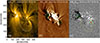 |
Fig. 1. (a) Observation of a sigmoidal loop (marked by the white dashed curve) associated with the pre-eruptive structure as seen in the AIA 171 Å channel. (b) Base difference image obtained from the AIA 193 Å channel. Green circles mark the two conjugate core-dimming regions observed during the eruption. (c) Line-of-sight component of the HMI magnetic field. The yellow dashed curve and the green circles are drawn in (a) and (b), respectively. The underlying magnetic polarities of the two conjugate core-dimming regions and the two ends of the sigmoidal loop are marked, indicating a northeast-directed left-handed flux rope. |
3.2.6. Magnetic helicity
Paper I featured a detailed analysis of the source AR of the CME, NOAA AR 12962. By employing the CB method (Georgoulis et al. 2012) for tracking the temporal evolution of the helicity budget of the region, we detected a net helicity difference of −7.1 ± 1.2 × 1041 Mx2 in its pre- and post-eruption phases. Assuming this difference in helicity is being transported to the associated CME, then the above is the helicity carried away by the CME, indicating a left-handed flux rope. This chirality aligns with the hemispheric helicity rule (Pevtsov et al. 1995, 2014) as the AR is located in the northern hemisphere and also with the morphological features of the structure as shown in Fig. 1.
3.2.7. Toroidal flux
To constrain the toroidal magnetic flux of the CME, we present a new method based on its helicity content. In this approach, we equate the near-Sun axial field strength (B0), derived from the helicity content of the CME, to the magnetic field strength (Bspheromak) at the spheromak’s magnetic axis. From the derived Bspheromak and the CME radius discussed in Sect. 3.2.4, we estimate the CME’s toroidal magnetic flux by following the method of Scolini et al. (2019), which assumes the magnetic field becomes completely axial at the spheromak magnetic axis in the linear force-free spheromak solution (Chandrasekhar & Kendall 1957; Shiota & Kataoka 2016; Verbeke et al. 2019). From Eq. (12) of Kataoka et al. (2009), the relation between the helicity of spheromak and its axial magnetic field is
 (2)
(2)
where H is the helicity content and a is the radius of the spheromak. As per Paper I and Sect. 3.2.6, H = −7.1 ± 1.2 × 1041 Mx2, while from Sect. 3.2.4, a = 8.34 ± 1.84 R⊙. This gives Bspheromak = 1178 ± 517 nT at the spheromak centre distance of 13.48 R⊙ (21.5 R⊙ − a). The uncertainty on Bspheromak is calculated by error propagation of the input parameters. Thus, the toroidal magnetic flux of the spheromak flux rope is estimated as 10.32 ± 6.35 × 10¹² Wb.
Since the estimated flux has an uncertainty range of more than 50%, we studied the influence of toroidal flux values on the simulation results, with the maximum limit being 16.7 × 10¹² Wb and the lower limit being 4 × 10¹² Wb with a mean value of 10.32 × 10¹² Wb. This is discussed in detail in Sect. 4.1.3.
4. Results
In Sect. 4.1, we iscuss the simulation results of the base run, plotted over in situ measurements by SolO and WIND at 0.43 AU and 0.99 AU, respectively. ThAn assessment of the effects of variations in density, insertion propagation direction, and toroidal flux in the simulation results follows this. In Sect. 4.2, the final simulation results at 0.43 AU and 0.99 AU, obtained with optimal parameters, are compared with in situ measurements by SolO and WIND, respectively. In Sect. 4.3, we analyse the CME’s magnetic field evolution up to 2 AU, aiming to derive the power-law index of the CME magnetic field magnitude variation. In Sect. 4.4, we compare and assess the effectiveness of our method to the PEA method.
4.1. Base run and effect of input parameters
Table 1 lists the CME input parameters obtained from Sect. 3.2. The simulation with these CME parameters is considered the base run. Fig. 2 (top to bottom) compares the magnetic field components, magnitude, and plasma parameters, such as number density and speed, from base simulation results recorded at 0.43 AU to in situ measurements at SolO. Similarly, Fig. 3 compares the modelled magnetic field components, magnetic field magnitude, and plasma parameters (e.g., number density and speed) from base-simulation results at 0.99 AU with in situ measurements from WIND.
Input parameters for the base EUHFORIA simulation.
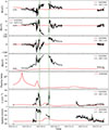 |
Fig. 2. Comparison of the base run results (model parameters in Table 1) with the in situ magnetic field components in the RTN system, magnetic field strength and plasma properties at 0.43 AU. Solid black curves denote the measurements from SolO, while solid red curves are the model outputs for the three components of the magnetic field (top three plots), the magnetic field strength (middle plot), and the plasma beta, number density and speed, respectively, in the bottom three plots. The vertical dashed green lines mark the estimated magnetic cloud boundaries. |
In both simulation results (at 0.43 AU and 0.99 AU), the base run fails to capture significant ICME milestones, such as shocks, ICME intervals, and MC boundaries discussed in Sect. 2. To improve the simulation results, we analyse how variations in density, insertion propagation direction, and toroidal flux affect simulation results at the two heliocentric distances. Fig. 4 illustrates base-run simulation results, showing the evolution of the CME in both the equatorial and meridional planes. From Fig. 4, at 09:59 UT on 12 March 2022, the CME is visible as a bipolar structure in Bz (panels a–b), with enhanced radial velocity (vr) in the same spatial region (panels e–f). The CME front is directed eastward of the Sun–Earth line, indicating that the main ejecta is not Earth-directed but propagates toward the sector where Solar Orbiter is located. The CME propagates towards the east with respect to the Sun-Earth line.
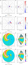 |
Fig. 4. Base simulation results showing the CME evolution in equatorial (left) and meridional (right) planes. Panels (a–d) display the magnetic field component Bz (nT). Panels (e–h) display the radial velocity Vr (km/s), at 2022-03-12 09:59 UT (a–b, e–f) and 2022-03-13 19:59 UT (c–d, g–h). Left panels (a, c, e, g) show a top-down view of the CME propagation on the equatorial plane, while the right-hand panels (b, d, f, h) show the meridional plane, giving a side-on view of its vertical extent and latitudinal structure. The concentric circles indicate heliocentric distance contours and serve as radial reference markers. |
By 13 March 2022 19:59 UT (panels c–d), the CME front has broadened, yet the strongest magnetic and velocity signatures remain eastward of Earth’s position. This spatial configuration implies that Earth encounters only the CME’s Eastern flank rather than its nose. Consequently, the simulated magnetic field and plasma parameters at Earth are weaker than those observed, indicating that the base run represents a flank encounter rather than a direct hit. Overall, the 2D visualisations provide valuable physical insight into the CME’s propagation behaviour. The comparison between the modelled CME front and spacecraft locations reveals that the apparent failure of the base run arises from a directional offset in the CME’s trajectory, leading to a missed impact at Earth.
We aim to improve the simulation results by investigating the dependence on CME input parameters, including density, propagation direction, and toroidal flux. In Sect. 4.1.1, we discuss how the simulation responds to different CME density inputs. The impact of the insertion direction is analysed in Sect. 4.1.2, followed by a discussion in Sect. 4.1.3 of simulation results using the upper and lower uncertainty limits, as well as the mean values of the estimated toroidal flux.
4.1.1. Effect of density
Figures 5 and 6 illustrate simulation results of the magnetic field and plasma parameters (from top to bottom), such as the number density (n) and speed, with density values listed in Table 2 overplotted with in situ measurements by SolO and WIND, respectively. For these runs, all other input parameters are kept as base run values except propagation direction and toroidal flux, which were kept as (0°,0°) and 1.66 × 10¹³ Wb, respectively. The procedure followed for obtaining these values is discussed in subsequent sections.
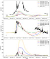 |
Fig. 5. Magnetic field strength (top panel), speed (middle), and density (bottom panel) of the ICME obtained from the model runs using different initial spheromak densities in units of kg m−3 plotted on top of the in situ measurements at 0.43 AU. |
Model runs with different CME density values for the CME spheromak model.
From Fig. 5, all simulation runs reproduce the overall ICME sequence, such as shock, sheath, and magnetic ejecta, but differ in how well they capture the timing and amplitude of each feature. The lowest density run D1 (1 × 10⁻¹⁸ kg m−3, blue) not only underestimates the shock signature but also fails to reproduce the magnetic ejecta structure, yielding magnetic field, speed, and density levels well below those observed. Increasing the CME density to 10 × 10−18 kg m−3 (D2, red) leads to a markedly improved representation of the full ICME profile: the shock and sheath arrival match the observed timing, the magnetic field enhancement agrees in magnitude, and both the speed and density evolution across the ejecta align closely with the in situ measurements. In contrast, the higher-density runs (30 × 10−18 kg m−3, D3 orange, and 60 × 10−18 kg m−3, D4 green) increasingly exaggerate the ICME signatures; they produce overly strong and broadened sheath regions and inflated density peaks within the ejecta, arriving earlier than observed. Overall, a CME density of 10 × 10−18 kg m−3 provides the most realistic reproduction of the observed magnetic and plasma parameters at SolO’s location, offering the best overall correspondence to the in situ measurements.
Similarly, from Fig. 6, all density-scaled runs reproduce the jump associated with the shock ahead of the ICME when compared with the in situ WIND measurements at 0.99 AU. The lowest density run (1 × 10⁻¹⁸ kg m−3, D1, blue) fails to reproduce the key CME signatures, strongly underestimating the magnetic field, speed, and density. The highest density run (60 × 10−18 kg m−3, D4, green) captures the peak density best but does so too early and significantly overestimates the magnetic field and speed. The intermediate-density run (30 × 10−18 kg m−3, D3, Orange) improves the overall match by aligning the shock timing more closely and reducing the overshoot. However, it still slightly overestimates both density and speed. In contrast, the 10 × 10−18 kg m−3, D2, red) provides the most balanced performance, closely matching the shock arrival time and offering a good representation of the magnetic field and speed profiles, while only modestly underestimating the density.
Hence, it is inferred that a density value ten times larger than the default density value of 10−18 kg m−3 better captures the magnetic field strength and other plasma parameter profiles at both vantage points. Hence, we fixed the density of our CME at 10 × 10−18 kg m−3.
4.1.2. Effect of propagation direction
Figures 7 and 8 (top to bottom) illustrate simulation results of the magnetic field components, magnitude, and plasma parameters, such as number density (n) and speed, with three insertion propagation directions namely, (0°,0°), (20.7°,7.8°), (6°,12°), and (16°,10°), with in situ measurements at 0.43 AU and 0.99 AU respectively. These different insertion direction runs are hereafter referred to as P1, P2, P3, and P4 as shown in Table 3. For these runs, all other input parameters are set to their base run values, but density is set as 10 × 10−18 kg m−3 as discussed above and toroidal flux is kept as and 1.66 × 10¹³ Wb, the procedure followed for choosing this value is discussed in the subsequent section.
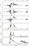 |
Fig. 7. Magnetic field components in the RTN system, magnetic field strength and plasma properties of the ICME obtained from the model runs with different insertion directions, namely, P1 (blue), P2 (red), P3 (cyan), and P4 (orange) plotted on top of the observed in situ values (black) at the SolO heliocentric distance of 0.43 AU. |
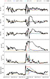 |
Fig. 8. Same as Fig. 7, but compared with in situ values at the WIND heliocentric distance of 0.99 AU. |
Model runs with different insertion propagation direction for the CME spheromak model.
From Fig. 7, we can see that all three simulation results have slight temporal shifts from each other and in situ measurements; however, all the correspondences in the comparisons below have been made on the basis of co-temporal in simulation-observation segments. In terms of magnetic field components, all runs fail to capture the polarity of Br, resulting in a direction opposite to that observed in the in situ measurements. The polarity is successfully reproduced for Bt and Br, and the P1 magnitude of the magnetic field closely matches in situ measurements. P2 fails to reproduce the key peaks and dips in both magnetic field magnitude and plasma parameters associated with shock arrival and MC regions, resulting in a less realistic representation of the ICME. P3 provides an intermediate result, capturing magnetic and plasma parameter variations more closely than P2, but these variations are still underestimated compared to P1. P4 provides results similar to P2 while producing a lower magnitude of magnetic field and other plasma parameters. In terms of n, the P1 simulation predicts a pronounced density enhancement that closely matches the observed peak, with good timing alignment with SolO measurements. P2 underestimates the density and fails to reproduce the observed variations. P3 follows the observed density trend more closely than P2, but it does not fully capture the peak density observed in P1. P4 also underestimates the density and fails to reproduce peaks similar to P2. However, the P1 simulation closely follows the observed trend for solar wind speed, capturing both the sharp rise and subsequent decline. The peak speed predicted by P1 is higher and better aligns with actual measurements.
In addition, both P4 and P2 underpredict solar wind speed increases, instead showing a gradual rise, which is inconsistent with the observed sharp transition. The P3 simulation predicts a peak speed slightly higher than the GCS case, but still falls short of matching the observed sharp transition. Overall, the P1 simulation results for (0° ,0° ) as the insertion direction provide the best representation of the ICME passage, particularly in capturing the solar wind speed, plasma density, and magnetic field magnitude.
Similarly, in Fig. 8 all four runs fail to reproduce the magnetic field components accurately, but better reproduce the magnetic field magnitude. While none of the insertion directions perfectly replicates the observed magnetic and plasma variations, the P1 results provide a better match than those of P2, P3, and P4. For n, the P1 simulation predicts a density enhancement that aligns well with the observed peak in timing. However, it slightly underestimates the maximum density value. The P2 results overestimate the density before ICME arrival, leading to an increase not observed in the in situ data. The P4 simulation shows a late density enhancement and an underestimated density. When analysing the solar wind speed, the P1 model closely follows the observed profile, accurately capturing the sharp rise at the ICME’s arrival and the gradual decline afterwards. The peak speed predicted by P1 is closer to the actual observed value, making it a better representation of the event.
In contrast, P2 underestimates the increase in speed. The P3 and P4 simulations fall between these two, providing a slightly steeper rise than GCS but not matching the observed steep velocity jump. This suggests that while (6° ,12° ) and (16° ,10° ) insertion directions offers an improvement over P2 results in capturing the speed profile, it remains less accurate than the (0° ,0° ) insertion direction simulation. Overall, the (0° ,0° ) insertion direction gives the most comparable results among the three tested insertion propagation directions at 21.5 R⊙ when compared with in situ measurements.
We further assess uncertainties in the CME deflection in latitude and longitude along its propagation path, accounting for deviations from the simulated CME trajectory. To do this, we placed multiple virtual spacecraft (VSCs) within 10°E–10°W and 10° N–10°S at 1 AU (as illustrated in Fig. 9). Adjacent VSCs are separated by 5° either longitudinally or latitudinally. We emphasise that these virtual spacecraft are used solely as sampling points to account for limitations in the simulation and are not intended to represent a change in the actual Earth position.
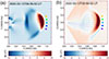 |
Fig. 9. Bz component of the spheromak in HEEQ coordinates shown on (a) the equatorial plane and (b) the meridional plane. The coloured dots indicate the locations of the virtual spacecraft at 1 AU. Adjacent spacecraft are longitudinally separated by 5°. The central dot (cyan) denotes the location of Earth. |
The comparison of simulation results obtained at different VSCs with in situ measurements at 0.99 AU is shown in Fig. 10. From this, we find that the VSC at (5°, 0°), indicated by the green dot in Fig. 9, provides the closest match to the in situ magnetic field measurements. This offset likely arises from small deviations in the simulated CME propagation due to interactions with the ambient solar wind and magnetic field structures, which can cause departures from a purely radial trajectory. For quantitative comparison with WIND measurements, we therefore use the VSC recording at (5°, 0°) at a radial distance of 1 AU. This analysis highlights the importance of multi-point observations in understanding ICME dynamics and demonstrates a practical approach to account for modelling uncertainties.
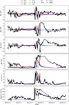 |
Fig. 10. Modelled magnetic field components in the GSE system, magnetic field strength and plasma properties, and the magnetic and plasma profiles (density and speed) obtained at the virtual spacecraft located within 10°E–10°W and 10° N–10° S at 1 AU plotted on top of WIND measurements. |
4.1.3. Effect of toroidal flux in magnetic field profile
Figures 11 and 12 (top to bottom) illustrate simulation results for the magnitude and plasma parameters, such as number density (n) and speed, with density values listed in the Table 4. For these, all other input parameters are kept as base run values except density and propagation direction, which are kept as 10 × 10−18 kg m−3 and (0°,0°) respectively as found optimal in Sect. 4.1.1 and Sect. 4.1.2.
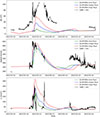 |
Fig. 11. Magnetic field strength (top panel), density (middle), and speed (bottom panel) of the ICME obtained from the model runs using different magnetic flux inputs plotted on top of the observed in situ measurements at 0.43 AU. |
Model runs with different toroidal flux values for the CME spheromak model.
In Fig. 11, we can see that the shock arrival time is well captured by all three simulations, regardless of the flux input. However, the magnitude of the toroidal flux significantly influences the simulated peaks. Higher flux levels better capture the observed peaks of the magnetic field, speed, and density. The maximum flux simulation (red curve) for magnetic field strength better matches the peak field strength observed in SolO measurements, even though the simulation underestimated the magnitude by 47%. The maximum-flux simulation reproduces the peak in the speed profile at shock arrival, consistent with the SolO measurements. For the density, the maximum flux input simulation results in a strong density peak at shock arrival, consistent with the SolO data. After the shock, the simulation result declines smoothly, whereas the in situ measured density decreases gradually.
Similarly, Fig. 12 compares the simulation results at 1 AU of |B| (top), solar wind speed (middle), and n (bottom) of different toroidal flux inputs derived in Sect. 3.2.7 (minimum, mean, and maximum) with in situ measurements at WIND. As in Fig. 11, the maximum flux produces higher peaks in |B|, speed, and n, while the minimum flux produces lower peaks. The timing of the shock arrival is well matched to the in situ data; however, the simulation results underestimate |B| by ∼20% even with the maximum magnetic flux. Solar wind speed also depends on the input flux, with higher flux leading to higher velocities, particularly near the shock arrival. The simulation results with maximum flux closely match the WIND speed trend at the shock arrival, but post-shock, the simulations show a more gradual decline compared to in situ measurements, which drop more sharply. Like speed, n shows a flux dependence where maximum flux produces significantly higher density peaks than the mean and minimum of toroidal flux. Post-shock simulation densities are higher than in situ measurements, which decline more rapidly.
The comparison of simulation results with SolO and WIND in situ measurements demonstrates that the maximum magnetic flux input in EUHFORIA simulations best matches the observed magnetic field strength, speed, and density. For both datasets, the maximum-flux simulation better captures the timing and shock-arrival peaks, particularly in terms of magnetic field and density, compared to the minimum- and mean-flux inputs.
4.2. Final simulation results and in situ comparison
Once we obtained all CME input parameters that reproduced the in situ measurements better, we went on to consider the optimal simulation results that best match the in situ observations from SolO and WIND. The optimised simulation parameters used for this final run are listed in Table 5. In previous studies, such as Samara et al. (2022), the Dynamic Time Warping (DTW) method was introduced to assess solar wind time series at L1, evaluating model performance and quantifying differences between observed and modelled time series. Maharana et al. (2024) used DTW to assess the capability of the toroidal modified Miller-Turner CME model in EUHFORIA to predict the critical Bz component of the CME’s magnetic field upon arrival at Earth. Here, however, there is no need for such a quantitative assessment since the effect of density, propagation direction, and toroidal flux on the arrival time and shock strength upon arrival is evident from the above analysis.
Input parameters for the final EUHFORIA simulation.
Fig. 13 compares the magnetic field components, magnitude, and plasma parameters, such as number density and speed, from simulation results recorded at 0.43 AU to in situ measurements at SolO. In Fig. 13, the simulation reasonably captures the overall structure of the ICME, including its elevated magnetic field strength and density. For the magnetic field components, the simulation captures the general directionality of Bt and Bn, except Br, where the polarity is captured in the opposite direction. However, the flux rope’s peak magnetic field magnitude is underestimated by 47% as seen in Sect. 4.1.3. The rotation of the Bt and Bn components (Bt transitioned from a positive to a negative value while Bn transitioned from a negative to a positive value) indicates the presence of an MC region, which further tends to progress towards the maximum magnetic field of an ICME, which is missed due to a data gap in SolO measurements. For the magnetic field magnitude, the simulation accurately captures the gradual increase and decrease in magnetic field strength during the event, exhibiting a reasonable time alignment with SolO. From Paper I, the estimated ICME |B| peak value from in situ measurements, employing data gap resolution methods of MAG/SolO in situ observations, is 109.72 ± 20.27 nT. From the simulation results, the peak magnetic field strength is underestimated by 47%. A temporal lag of 4 h and 40 minutes is observed between the front edge of the observed and modelled flux rope, even though the simulation captures the shock arrival time. This can be attributed to the non-distinguishable sheath and flux-rope boundary due to the compression effect at the front in the high-density run, as discussed in Sect. 3.2.1. In terms of plasma properties, the simulation successfully captures the overall density variations. The solar wind speed trend is well reproduced, with an increase preceding the ICME event and a gradual decline following it. Overall, the simulation results reasonably approximate the ICME’s structure and timing at 0.43 AU.
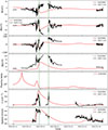 |
Fig. 13. Comparison of the model results (model parameters in Table 5) with the in situ magnetic field components in the RTN system, magnetic field strength and plasma properties at 0.43 AU. The black solid curves denote the measurements from SolO, while the red solid curves are model outputs for the three components of the magnetic field (top three plots), the magnetic field strength (middle plot), and the plasma beta, number density and speed, respectively (bottom three plots). The vertical green dashed lines mark the estimated magnetic cloud boundaries, within which the plasma beta becomes less than 1 in the simulation results. |
In Fig. 14, we compare the modelled magnetic field components, magnitude, and plasma parameters such as number density and speed, with parameters listed in Table 5 with in situ measurements by WIND. The simulation reasonably captures the overall structure of the ICME, including its elevated magnetic field strength and density. For the magnetic field components (top three plots in Fig. 14), in in situ measurements, there was a rotation of Bz as it shifted from northward to southward and By from east to west – a characteristic of an MC. However, in the simulation results, Bz shows a gradual shift but fails to reproduce the sharp rotation observed in the in situ data. The transition in the simulation appears much smoother and less pronounced, lacking the clear northward-to-southward swing seen in the measurements. The simulated By does capture a partial rotation, but it is less well-defined and occurs more gradually compared to the in situ data. The Bx component, however, is reasonably reproduced. The fourth panel displays the |B| value. The simulation captures the overall increase and subsequent decline in field strength, roughly aligning with the in situ data. The measured magnetic field strength reaches 24.41 ± 0.05 nT, and the simulation predicts 19.62 nT, underestimating the field strength by approximately 20%. Similar to the 0.43 AU simulation results, at 1 AU, the sheath region is less profound, making it challenging to discern between the sheath region and the MC region in the simulation results, even though the shock arrival time is well reproduced. In the fifth panel, illustrating plasma beta variation, the simulation overestimates plasma beta during the MC region, but it still drops below 1. In the sixth panel showing plasma density, the simulation captures the general trend: a sharp increase at the shock, followed by a decline, even though the density is lower for most of the MC. In the final panel showing solar wind speed, the simulation reproduces the overall speed profile, with a sharp increase at the shock and a gradual decline during the ICME passage. However, the quasi-linear decrease in the radial speed of the ICME with time mostly follows the expansion of the ejecta in observation. This difference suggests that the model does not fully capture the deceleration of the ICME in the solar wind. Overall, the EUHFORIA simulation reasonably approximates the ICME structure, including the peak magnetic field strength at 0.99 AU and the MC boundaries.
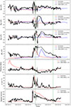 |
Fig. 14. Same as Fig. 13, but for WIND data at 0.99 AU. The blue solid lines in the top four plots are the same as the model output, indicated by the red solid lines, but shifted by 15 hours and 48 minutes so that the front edge of both the observed and modelled flux rope temporally coincides. |
4.3. Power-law variation of magnetic field strength from modelling results
In this section, we analyse the CME’s magnetic field evolution up to 2 AU, aiming to infer a single power-law index of CME magnetic field radial evolution. As CMEs propagate in the heliosphere, their magnetic field magnitude decreases with increasing distance from the Sun and subsequent expansion. Several previous studies, such as those of Bothmer & Schwenn (1997), Wang et al. (2005), Farrugia et al. (2005), Démoulin & Dasso (2009), Winslow et al. (2015), Patsourakos et al. (2016) and Paper I, have found that this decrease is close to being self-similar, hence the total magnetic field magnitude can be expected to decay with heliocentric distance D with an index of αB, expressed as
 (3)
(3)
By simulating the CME using optimal input parameters collected in the Table 5 from 21.5 R⊙ to 2 AU, we recorded the maximum magnetic field magnitude at distances ranging between 0.2 AU and 2 AU with a step of 0.2 AU. Fig. 15 illustrates this variation and a linear (power-law) regression from 21.5 R⊙ to 2 AU. The least-squares best fit gives a power-law index α = −1.63 ± 0.06. A more detailed discussion of this result, including a comparison with prior studies in this direction, is presented in Sect. 5.
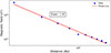 |
Fig. 15. CME magnetic field magnitude as a function of distance from 0.2 AU to 2 AU from final simulation results in log-log scale. The red line represents the least-squares power-law best fit. |
4.4. Comparison of effectiveness of our method with the PEA method
To compare our simulation results, obtained by constraining the toroidal flux from the CME’s helicity budget, with the PEA method of Gopalswamy et al. (2017), for this particular CME, we identified a fully formed PEA in source AR in over 6 h following the eruption. Applying the method described by Gopalswamy et al. (2017) to the AIA 193 Å image on a fully formed PEA on 11 March at 01:57 UT, we identified the PEA area, assumed to be where magnetic reconnection has occurred. Under this assumption, we calculate the total (unsigned) magnetic flux over the PEA area from the line-of-sight HMI magnetogram on 11 March at 02:00 UT. Dividing it by two gives the approximate (signed) reconnected flux. Hence, we estimated the reconnected magnetic flux in the PEA region as 5 × 10¹³ Wb. Assuming that all reconnected flux goes into the poloidal magnetic flux of the erupted flux rope, following Scolini et al. (2019), we estimated the spheromak axial magnetic field as 4860 nT and the flux-rope toroidal magnetic flux bounded by the spheromak of radius of 8.34 R⊙ as 4.18 × 10¹³ Wb. A simulation run with this PEA-obtained toroidal flux compared with our helicity-based estimated toroidal flux of 4 − 16.7 × 10¹² Wb is illustrated in Fig. 16. These runs included all other optimal input parameters listed in Table 5.
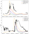 |
Fig. 16. Magnetic field strength of the ICME obtained from the model runs using different magnetic flux inputs from our methodology, and PEA estimated flux plotted against the in situ measurements at 0.43 AU (top) and 0.99 AU (bottom). |
From Fig. 16, it can be seen that the PEA method slightly better predicts the CME magnetic field magnitude at 0.43 AU and 0.99 AU, with a 13% overestimation of the peak magnetic field magnitude at both heliocentric distances. The comparison between the helicity-based and PEA methods is discussed further in some detail in Sect. 5.
5. Discussion and conclusions
In this study, we introduce a new approach to constraining the magnetic flux of a CME within the spheromak model, utilising the near-Sun magnetic field of the CME derived from its helicity content following the methodology in Patsourakos et al. (2016). This approach is implemented in EUHFORIA, an inner-heliospheric MHD CME-propagation model. To validate the method’s results, we simulated the magnetic field evolution of a CME launched from the Sun on 10 March 2022, from 21.5 R⊙ to 2 AU. The advantageous multi-spacecraft in situ measurements, one at the inner heliosphere, approximately mid-Sun-Earth line, at 0.43 AU, and another at 0.99 AU, offered a valuable opportunity to constrain the simulation’s input parameters and validate the simulated magnetic field components and plasma parameters.
With our approach, we were able to constrain the CME magnetic flux using its helicity budget. The estimated axial magnetic field at the centre distance of 13.48 R⊙ is 1178 ± 517 nT. The corresponding toroidal magnetic flux of this CME bounded with a spheromak radius of 8.34 ± 1.84 R⊙ is 10.32 ± 6.35 × 10¹² Wb. The comparison of in situ spacecraft measurements at two vantage points, one at 0.43 AU and the other at 0.99 AU, with simulation results, reveals that the model using the magnetic flux derived from the CME helicity budget successfully reproduces key aspects of the CME structure, including the shock arrival time and signatures of MC such as rotation of the magnetic field components. In situ measurements at 0.43 AU have proven particularly valuable in optimising predictions at L1. Specifically, the availability of density and speed measurements midway along the Sun-Earth line helps optimise CME properties to match SolO measurements, synchronising with the arrival time at WIND at L1. This aligns with the studies that utilised multi-point observations, such as the results by Sarkar et al. (2024), which utilised measurements at an inner spacecraft to tighten estimates of flux-rope orientation, impact distance, and axial field strength. These results, in turn, sharply reduced the parameter uncertainty and enabled highly accurate prediction of the magnetic field at the next spacecraft, achieving correlations of 90% between simulated and observed Bz at the outer location. Consistent findings across earlier studies reinforce this advantage. For instance, Möstl (2018) showed that tracking the same ICME with radially aligned spacecraft improves magnetic structure reconstruction and reduces ambiguity in model fits; Good et al. (2019a) found that inner–outer comparisons allow models to better capture rotation and expansion; and Weiss (2021) demonstrated that multi-point data help identify departures from self-similar expansion, preventing systematic underestimation of field strength at larger distances. This reinforces the importance of studying events with multi-spacecraft observations to improve space weather modelling at Earth.
In Paper I, we derived the power-law index governing the variation of the maximum magnetic field magnitude of this CME with heliocentric distance as αB = −1.23 ± 0.18, based on just three data points from 0.03 AU to 1 AU. This improved upon previous studies that typically considered the 0.3–1 AU range. This result closely aligns with studies incorporating near-Sun magnetic field data, for instance, the Parker Solar Probe observations reported in Salman et al. (2024). Using 3D MHD simulation results, in this work, we extended this analysis to a broader range from 21.5 R⊙ to 2 AU and obtained a steeper and more robust index of αB = −1.63 ± 0.06. This result is consistent, within the uncertainty limits, with previous studies on various CMEs over similar distances of 0.03–1 AU, such as (Leitner et al. 2007; Démoulin & Dasso 2009; Good et al. 2019b; Salman et al. 2020) and Patsourakos & Georgoulis (2016). Additionally, Scolini et al. (2021), who analysed the 12 July 2012 CME using EUHFORIA simulations up to 2 AU, reported an even steeper fall-off with αB = −1.9. These differences in αB values suggest that a single power-law index may not accurately represent magnetic field evolution across all CMEs, as the profile can vary significantly with event characteristics. This underscores the need for comprehensive statistical studies to better characterise the heliocentric evolution of CME magnetic fields.
Overall, although the simulations reasonably capture the ICME structure and arrival time at recorded distances, specific challenges in modelling must be acknowledged. There is an underestimation of peak magnetic field strength by approximately 47% at 0.43 AU and a corresponding underestimation of 19% at 0.99 AU. The improved agreement between the model and observations at larger heliocentric distances may be attributed to the extended propagation of the CME, which allows for increased interactions with the ambient solar wind. In contrast, closer to the Sun, the results may be more sensitive to the initial conditions, which (as is commonly acknowledged) tend to be relatively idealised. Furthermore, as discussed in Sect. 4.1.1, higher density values than the default in EUHFORIA produce a stronger magnetic field, which better matches in situ measurements. However, the higher density simulation results for the event under study fail to reproduce the sheath region of the ICME. As seen in Sect. 4.1.2, comparing simulation results with different propagation directions at the time of insertion suggests that a GCS-fitted height measurement does not necessarily provide accurate information on CME orientation at the model insertion distance. This is because such measurements correspond to the CME’s orientation at near-Sun distances (here, 7.6 R⊙), rather than at the insertion distance (21.5 R⊙). As discussed in Sect. 4.1.2, data from STEREO’s heliospheric imager, which has a field of view extending beyond coronagraphs, can offer valuable insights for refining our understanding of CME orientation. Apart from the uncertainties related to constraining the input tilt of the CME at the inner boundary (21.5 R⊙) of the heliospheric model, the spheromak tilting instability poses an additional limitation in modelling the CME orientation in the heliospheric domain (Asvestari et al. 2022; Sarkar et al. 2024). In particular, fully inserted spheromaks in the heliospheric domain may undergo significant rotation (Asvestari et al. 2022). Moreover, because fully inserted spheromak-type CME models lack attached legs at the heliospheric model’s inner boundary, the trailing part of the structure exhibits an unrealistic magnetic field profile. It is also worth noting that magnetic field strength simulation results depend on the input magnetic flux. The magnetic flux derived using our methodology exhibits a wide uncertainty limit of approximately 50%, and the maximum magnetic flux input best matches all observed magnetic field strength, speed, and density parameters.
From the comparison study of our helicity-based method in constraining magnetic flux for predicting the magnetic field strength at L1, as seen in Sect. 4.4, for the event studied, the PEA method better predicts the CME magnetic field magnitude both at 0.43 AU and at 0.99 AU, with a slight overestimation of the peak magnetic field magnitude by 13% at both heliocentric distances. However, in the PEA-based method, the area used to estimate the flux from the HMI magnetogram is larger than the area corresponding to the footpoints directly involved in the reconnection, potentially leading to an overestimation of the reconnected flux. The discrepancy in reconnected flux, compared to the ribbon-observation method of Kazachenko et al. (2017), is a factor of 2 smaller, as reported in Gopalswamy et al. (2017) when comparing the two methods. Additionally, Zhang et al. (2021) compared the helicity-based method of Patsourakos & Georgoulis (2016) and the method of Gopalswamy et al. (2017) for estimating the near-Sun CME axial magnetic fields at 10 R⊙. The results suggest a broad distribution spanning up to 12 500 nT. The Patsourakos & Georgoulis (2016) results show a peak probability density of magnetic fields of ∼3000 nT at 10 R⊙, while the Gopalswamy et al. (2017) method suggests a stronger field, with a median of 5900 nT and an average of 5190 nT.
While both approaches show some overlap, the helicity-based method generally predicts weaker fields. The PEA method yields the highest estimate of reconnected flux, leading to an overestimation of the magnetic field magnitude. In previous studies aimed at constraining the CME toroidal flux from the PEA method, these higher fluxes were used to match in situ measurements. As seen in Fig. 16, our simulation results, which constrain toroidal flux with a helicity budget, lie somewhat between the two in terms of forecasting magnetic field magnitude. This method underestimates the peak magnetic field strength but provides quantitative estimates of chirality, yielding moderately reliable results. Notably, the PEA method estimates reconnection flux by measuring the magnetic flux underlying the final arcade footprint (Qiu et al. 2007; Gopalswamy et al. 2018), but this approach carries several implicit assumptions. It assumes that the arcade fully covers the region involved in reconnection and represents the cumulative effect of ribbon separation (Longcope et al. 2007), the flare has a largely bipolar magnetic configuration (Forbes & Lin 2000), and that the bright arcade loops correspond primarily to newly reconnected field lines rather than pre-existing coronal structures (Kazachenko et al. 2017). The method further relies on the idea that a single late-phase arcade image adequately reflects the entire reconnection history (Qiu & Cheng 2022) and that photospheric line-of-sight magnetic field measurements provide a reasonable approximation of the true flux beneath the arcade, particularly for near-disk-centre events (Priest 2014). In addition, it presumes that the erupting flux rope is mainly built during the flare and that its magnetic content is not substantially modified afterwards, an assumption consistent with standard CME-flare models (Lin et al. 2004), but not necessarily with events involving gradual pre-eruptive flux-rope formation (Green et al. 2018; Patsourakos et al. 2020). As a result, PEA-based estimates effectively capture only the poloidal flux added during flare reconnection. They cannot account for magnetic flux that may have existed in a pre-eruptive flux rope, leading to potential underestimation of the total magnetic content of the CME in such cases (Patsourakos et al. 2020). In contrast, helicity-based methods do not rely on the assumption that the flux rope is formed entirely during the flare and can incorporate both pre-eruptive and flare-added components, making them applicable to a broader range of eruptive events, including those involving well-developed pre-existing flux ropes (Nindos et al. 2003; Petrie 2020; Thalmann et al. 2021).
Furthermore, irrespective of the method used to estimate the reconnection flux, uncertainties in translating this flux into the poloidal flux of the analytical flux rope (represented as a spheromak in this study) also affect the resulting magnetic field strength of the flux rope. One source of uncertainty comes from estimating the spheromak radius because if the spheromak is larger than assumed, the magnetic field strength corresponding to a given reconnection (or poloidal) flux may be underestimated. The spheromak geometry differs significantly from that of the GCS model and the spheromak radius must therefore be constrained using the average of the face-on and edge-on angular widths obtained from the GCS model, which itself involves large uncertainties in determining the CME geometry. Additional uncertainties arise from pressure imbalance conditions when the CME is inserted into the heliospheric domain in EUHFORIA. In other words, if the model underestimates the background solar wind pressure, the flux rope may undergo overexpansion during the insertion phase until it reaches pressure balance with the background solar wind, leading once again to an underestimation of the magnetic field strength relative to in situ observations. Owing to these uncertainties, even if the PEA method appears to yield slightly better results in this study, it remains difficult to prioritise one approach over another among the PEA (Gopalswamy et al. 2017), ribbon-observation (Kazachenko et al. 2017), and helicity-based methods (Patsourakos & Georgoulis 2016), particularly when the analysis is limited to a single event, as in this work.
A study such as this, with a detailed comparison of different methods to constrain the toroidal flux performed on a statistically significant set of events, would be highly valuable for optimising the methodology to improve prediction accuracy and clarify the relationships among flux-constraining approaches, such as helicity-based, PEA, and ribbon methods. Based on these insights, it will be meaningful in future work to explore hybrid methods that combine appropriate features from both PEA and helicity-based approaches, thereby enabling more robust and event-specific predictions. In addition, a comprehensive statistical investigation covering a broader range of CME models beyond the spheromak, such as the FRi3D flux rope CME model (Maharana et al. 2022), the spheroid CME model (Scolini et al. 2024), and the Toroidal/Modified Miller–Turner/horseshoe CME model (Maharana et al. 2024), is required. Incorporating diverse CME events observed by multiple spacecraft could yield robust, widely applicable conclusions on the reliability, efficiency, and compatibility of the helicity-based method relative to other approaches. Such an investigation will also help assess the method’s compatibility with other CME models, offering valuable guidelines for future modelling efforts.
Acknowledgments
The authors thank the anonymous referee for constructive suggestions and insightful comments that have significantly improved the manuscript. This work is part of the SWATNet project funded by the European Union’s Horizon 2020 research and innovation programme under the Marie Skłodowska-Curie grant agreement No 955620. This research also acknowledges the funding from the European Union’s Horizon 2020 research and innovation program under grant agreement No. 870405 (EUHFORIA 2.0). We also appreciate the availability of open-source data from the Solar Orbiter and WIND spacecraft, accessible via the Coordinated Data Analysis Web (https://cdaweb.gsfc.nasa.gov/index.html). R. Sarkar acknowledges support from the project EFESIS, under the Academy of Finland Grant 350015. A. Nindos and S. Patsourakos acknowledge support from the ERC Synergy Grant ‘Whole Sun’ (GAN: 810218). S. Poedts is funded by the European Union. Views and opinions expressed are, however, those of the author(s) only and do not necessarily reflect those of the European Union or ERCEA. Neither the European Union nor the granting authority can be held responsible. S. Poedts is funded via the project Open SESAME under the Horizon Europe programme (ERC-AdG agreement No 101141362), and the projects C16/24/010 C1 project Internal Funds KU Leuven, G0B5823N and G002523N (WEAVE) (FWO-Vlaanderen), and 4000145223 (SIDC Data Exploitation (SIDEX2), ESA Prodex).
References
- Asvestari, E., Pomoell, J., Kilpua, E., et al. 2021, A&A, 652, A27 [NASA ADS] [CrossRef] [EDP Sciences] [Google Scholar]
- Asvestari, E., Rindlisbacher, T., Pomoell, J., & Kilpua, E. K. J. 2022, ApJ, 926, 87 [NASA ADS] [CrossRef] [Google Scholar]
- Berger, M. A. 1984, Geophys. Astrophys. Fluid Dyn., 30, 79 [NASA ADS] [CrossRef] [Google Scholar]
- Bothmer, V., & Schwenn, R. 1997, Ann. Geophys., 16, 1 [Google Scholar]
- Burlaga, L., Sittler, E., Mariani, F., & Schwenn, R. 1981, J. Geophys. Res. (Space Phys.), 86, 6673 [NASA ADS] [CrossRef] [Google Scholar]
- Chandrasekhar, S., & Kendall, P. C. 1957, ApJ, 126, 457 [Google Scholar]
- Chen, P. F. 2011, Liv. Rev. Sol. Phys., 8, 1 [Google Scholar]
- Davies, J. A., Perry, C. H., Trines, R. M. G. M., et al. 2013, ApJ, 777, 167 [Google Scholar]
- Démoulin, P., & Dasso, S. 2009, A&A, 498, 551 [Google Scholar]
- Farrugia, C. J., Leiter, M., Biernat, H. K., et al. 2005, ESA SP, 592, 723 [Google Scholar]
- Forbes, T. G. 2000, J. Geophys. Res. (Space Phys.), 105, 23153 [Google Scholar]
- Forbes, T. G., & Lin, J. 2000, J. Atmos. Sol.-Terr. Phys., 62, 1499 [Google Scholar]
- Georgoulis, M. K., Tziotziou, K., & Raouafi, N.-E. 2012, ApJ, 759, 1 [NASA ADS] [CrossRef] [Google Scholar]
- Good, S. W., Forsyth, R. J., Phan, T. D., & Eastwood, J. P. 2019a, J. Geophys. Res. (Space Phys.), 124, 4960 [NASA ADS] [CrossRef] [Google Scholar]
- Good, S. W., Kilpua, E. K. J., LaMoury, A. T., et al. 2019b, J. Geophys. Res. (Space Phys.), 124, 4960 [NASA ADS] [CrossRef] [Google Scholar]
- Gopalswamy, N., Lara, A., Yashiro, S., Kaiser, M. L., & Howard, R. A. 2001, J. Geophys. Res., 106, 29207 [NASA ADS] [CrossRef] [Google Scholar]
- Gopalswamy, N., Yashiro, S., Akiyama, S., & Xie, H. 2017, Sol. Phys., 292, 65 [NASA ADS] [CrossRef] [Google Scholar]
- Gopalswamy, N., Yashiro, S., Akiyama, S., et al. 2018, J. Atmos. Sol.-Terr. Phys., 180, 35 [Google Scholar]
- Goto, M., Carmona, A., Linz, H., et al. 2012, ApJ, 748, 6 [NASA ADS] [CrossRef] [Google Scholar]
- Green, L. M., Török, T., Vršnak, B., Manchester, W., & Veronig, A. 2018, Space Sci. Rev., 214, 46 [Google Scholar]
- Halain, J. P., Berghmans, D., Seaton, D. B., et al. 2013, Sol. Phys., 286, 67 [NASA ADS] [CrossRef] [Google Scholar]
- Horbury, T. S., O’Brien, H., Carrasco Blazquez, I., et al. 2020, A&A, 642, A9 [NASA ADS] [CrossRef] [EDP Sciences] [Google Scholar]
- Howard, R. A., Moses, J. D., Vourlidas, A., et al. 2008, Space Sci. Rev., 136, 67 [NASA ADS] [CrossRef] [Google Scholar]
- Kaiser, M. L., Kucera, T. A., Davila, J. M., et al. 2008, Space Sci. Rev., 136, 5 [Google Scholar]
- Kataoka, R., Ebisuzaki, T., Kusano, K., et al. 2009, J. Geophys. Res. (Space Phys.), 114, A10102 [NASA ADS] [Google Scholar]
- Kazachenko, M. D., Lynch, B. J., Welsch, B. T., & Sun, X. 2017, ApJ, 845, 49 [NASA ADS] [CrossRef] [Google Scholar]
- Koya, S., Patsourakos, S., Georgoulis, M. K., & Nindos, A. 2024, A&A, 690, A233 [NASA ADS] [CrossRef] [EDP Sciences] [Google Scholar]
- Leitner, M., Farrugia, C. J., Möstl, C., et al. 2007, J. Geophys. Res. (Space Phys.), 112, A06113 [Google Scholar]
- Lemen, J. R., Title, A. M., Akin, D. J., et al. 2012, Sol. Phys., 275, 17 [Google Scholar]
- Lepping, R. P., Jones, J. A., & Burlaga, L. F. 1990, J. Geophys. Res. (Space Phys.), 95, 11957 [Google Scholar]
- Lepping, R. P., Acũna, M. H., Burlaga, L. F., et al. 1995, Space Sci. Rev., 71, 207 [Google Scholar]
- Lin, J., Raymond, J. C., & van Ballegooijen, A. A. 2004, ApJ, 602, 422 [NASA ADS] [CrossRef] [Google Scholar]
- Liokati, E., Nindos, A., & Liu, Y. 2022, A&A, 662, A6 [NASA ADS] [CrossRef] [EDP Sciences] [Google Scholar]
- Liokati, E., Nindos, A., & Georgoulis, M. K. 2023, A&A, 672, A38 [NASA ADS] [CrossRef] [EDP Sciences] [Google Scholar]
- Liu, Y., Welsch, B. T., Valori, G., et al. 2023, ApJ, 942, 27 [NASA ADS] [CrossRef] [Google Scholar]
- Longcope, D. W., Beveridge, C., Qiu, J., et al. 2007, Sol. Phys., 244, 45 [Google Scholar]
- Low, B. C. 1994, Phys. Plasmas, 1, 1684 [Google Scholar]
- Maharana, A., Isavnin, A., Scolini, C., et al. 2022, Adv. Space Res., 70, 1641 [NASA ADS] [CrossRef] [Google Scholar]
- Maharana, A., Linan, L., Poedts, S., & Magdalenić, J. 2024, A&A, 691, A146 [NASA ADS] [CrossRef] [EDP Sciences] [Google Scholar]
- Möstl, C., Amerstorfer, T., Palmerio, E., et al. 2018, Space Weather, 16, 216 [Google Scholar]
- Nindos, A., & Andrews, M. D. 2004, ApJ, 616, L175 [NASA ADS] [CrossRef] [Google Scholar]
- Nindos, A., Zhang, H., & Zhang, M. 2003, ApJ, 594, 1033 [Google Scholar]
- Ogilvie, K. W., Chornay, D. J., Fritzenreiter, R. J., et al. 1995, Space Sci. Rev., 71, 55 [Google Scholar]
- Owen, C. J., Bruno, R., Livi, S., et al. 2020, A&A, 642, A16 [EDP Sciences] [Google Scholar]
- Park, S.-H., Lee, J., Choe, G. S., et al. 2008, ApJ, 686, 1397 [NASA ADS] [CrossRef] [Google Scholar]
- Park, S.-H., Chae, J., & Wang, H. 2010, ApJ, 718, 43 [NASA ADS] [CrossRef] [Google Scholar]
- Patsourakos, S., & Georgoulis, M. K. 2016, A&A, 595, A121 [NASA ADS] [CrossRef] [EDP Sciences] [Google Scholar]
- Patsourakos, S., Georgoulis, M., Vourlidas, A., et al. 2016, ApJ, 817, 14 [NASA ADS] [CrossRef] [Google Scholar]
- Patsourakos, S., Vourlidas, A., Török, T., et al. 2020, Space Sci. Rev., 216, 131 [Google Scholar]
- Pesnell, W. D., Thompson, B. J., & Chamberlin, P. C. 2012, Sol. Phys., 275, 3 [Google Scholar]
- Petrie, G. 2020, Liv. Rev. Sol. Phys., 17, 5 [NASA ADS] [CrossRef] [Google Scholar]
- Pevtsov, A. A., Canfield, R. C., & Metcalf, T. R. 1995, ApJ, 440, L109 [NASA ADS] [CrossRef] [Google Scholar]
- Pevtsov, A. A., Berger, M. A., Nindos, A., Norton, A. A., & van Driel-Gesztelyi, L. 2014, Space Sci. Rev., 186, 285 [NASA ADS] [CrossRef] [Google Scholar]
- Pomoell, J., & Poedts, S. 2018, J. Space Weather Space Clim., 8, A35 [NASA ADS] [CrossRef] [EDP Sciences] [Google Scholar]
- Priest, E. 2014, Magnetohydrodynamics of the Sun (Cambridge University Press) [Google Scholar]
- Qiu, J., & Cheng, J. 2022, Front. Astron. Space Sci., 9, 877473 [Google Scholar]
- Qiu, J., Hu, Q., Howard, T. A., & Yurchyshyn, V. B. 2007, ApJ, 659, 758 [Google Scholar]
- Rochus, P., Auchère, F., Berghmans, D., et al. 2020, A&A, 642, A8 [NASA ADS] [CrossRef] [EDP Sciences] [Google Scholar]
- Rust, D. M., & Kumar, A. 1996, ApJ, 464, L199 [NASA ADS] [CrossRef] [Google Scholar]
- Sachdeva, N., Subramanian, P., Colaninno, R., & Vourlidas, A. 2015, ApJ, 809, 158 [NASA ADS] [CrossRef] [Google Scholar]
- Salman, T. M., Winslow, R. M., & Lugaz, N. 2020, J. Geophys. Res. (Space Phys.), 125, e27084 [NASA ADS] [Google Scholar]
- Salman, T. M., Nieves-Chinchilla, T., Jian, L. K., et al. 2024, ApJ, 966, 118 [NASA ADS] [CrossRef] [Google Scholar]
- Samara, E., Laperre, B., Kieokaew, R., et al. 2022, ApJ, 927, 187 [NASA ADS] [CrossRef] [Google Scholar]
- Sarkar, R., Pomoell, J., Kilpua, E., et al. 2024, ApJS, 270, 18 [NASA ADS] [CrossRef] [Google Scholar]
- Scolini, C., Rodriguez, L., Mierla, M., Pomoell, J., & Poedts, S. 2019, A&A, 626, A122 [NASA ADS] [CrossRef] [EDP Sciences] [Google Scholar]
- Scolini, C., Dasso, S., Rodriguez, L., Zhukov, A. N., & Poedts, S. 2021, A&A, 649, A69 [NASA ADS] [CrossRef] [EDP Sciences] [Google Scholar]
- Scolini, D., Verbeke, C., Pomoell, J., & Poedts, S. 2024, J. Space Weather Space Clim., 14, 14 [Google Scholar]
- Seaton, D. B., Berghmans, D., Nicula, B., et al. 2013, Sol. Phys., 286, 43 [NASA ADS] [CrossRef] [Google Scholar]
- Shiota, D., & Kataoka, R. 2016, Space Weather, 14, 56 [CrossRef] [Google Scholar]
- Stamkos, S., Patsourakos, S., Vourlidas, A., & Daglis, I. A. 2023, Sol. Phys., 298 [Google Scholar]
- Tappin, S. J. 2006, Sol. Phys., 233, 233 [NASA ADS] [CrossRef] [Google Scholar]
- Thalmann, J. K., Linan, L., Pariat, E., Valori, G., & Dalmasse, K. 2021, ApJ, 909, 113 [Google Scholar]
- Thernisien, A. F. R., Howard, R. A., & Vourlidas, A. 2006, ApJ, 652, 763 [Google Scholar]
- Thernisien, A., Howard, R., & Vourlidas, A. 2008, ApJ, 652, 763 [Google Scholar]
- Verbeke, C., Pomoell, J., & Poedts, S. 2019, A&A, 627, A111 [NASA ADS] [CrossRef] [EDP Sciences] [Google Scholar]
- Vourlidas, A., Patsourakos, S., & Savani, N. P. 2019, Phil. Trans. R. Soc. A, 377, 20180096 [Google Scholar]
- Wang, C., Du, D., & Richardson, J. D. 2005, J. Geophys. Res. (Space Phys.), 110 [Google Scholar]
- Webb, D. F., & Howard, T. A. 2012, Liv. Rev. Sol. Phys., 9, 3 [Google Scholar]
- Weiss, A. J., Möstl, C., Davies, E. E., et al. 2021, A&A, 656, A13 [NASA ADS] [CrossRef] [EDP Sciences] [Google Scholar]
- Winslow, R. M., Lugaz, N., Philpott, L. C., et al. 2015, J. Geophys. Res. (Space Phys.), 120, 6101 [NASA ADS] [CrossRef] [Google Scholar]
- Zhang, J., Temmer, M., Gopalswamy, N., et al. 2021, Prog. Earth Planet. Sci., 8, 56 [CrossRef] [Google Scholar]
- Zhuang, B., Lugaz, N., Al-Haddad, N., et al. 2024, A&A, 682, A107 [NASA ADS] [CrossRef] [EDP Sciences] [Google Scholar]
- Zurbuchen, T. H., & Richardson, I. G. 2006, Space Sci. Rev., 123, 31 [Google Scholar]
All Tables
Model runs with different insertion propagation direction for the CME spheromak model.
All Figures
|
Fig. 1. (a) Observation of a sigmoidal loop (marked by the white dashed curve) associated with the pre-eruptive structure as seen in the AIA 171 Å channel. (b) Base difference image obtained from the AIA 193 Å channel. Green circles mark the two conjugate core-dimming regions observed during the eruption. (c) Line-of-sight component of the HMI magnetic field. The yellow dashed curve and the green circles are drawn in (a) and (b), respectively. The underlying magnetic polarities of the two conjugate core-dimming regions and the two ends of the sigmoidal loop are marked, indicating a northeast-directed left-handed flux rope. |
| In the text | |
|
Fig. 2. Comparison of the base run results (model parameters in Table 1) with the in situ magnetic field components in the RTN system, magnetic field strength and plasma properties at 0.43 AU. Solid black curves denote the measurements from SolO, while solid red curves are the model outputs for the three components of the magnetic field (top three plots), the magnetic field strength (middle plot), and the plasma beta, number density and speed, respectively, in the bottom three plots. The vertical dashed green lines mark the estimated magnetic cloud boundaries. |
| In the text | |
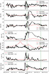 |
Fig. 3. Same as Fig. 2 but for WIND data at 0.99 AU. |
| In the text | |
|
Fig. 4. Base simulation results showing the CME evolution in equatorial (left) and meridional (right) planes. Panels (a–d) display the magnetic field component Bz (nT). Panels (e–h) display the radial velocity Vr (km/s), at 2022-03-12 09:59 UT (a–b, e–f) and 2022-03-13 19:59 UT (c–d, g–h). Left panels (a, c, e, g) show a top-down view of the CME propagation on the equatorial plane, while the right-hand panels (b, d, f, h) show the meridional plane, giving a side-on view of its vertical extent and latitudinal structure. The concentric circles indicate heliocentric distance contours and serve as radial reference markers. |
| In the text | |
|
Fig. 5. Magnetic field strength (top panel), speed (middle), and density (bottom panel) of the ICME obtained from the model runs using different initial spheromak densities in units of kg m−3 plotted on top of the in situ measurements at 0.43 AU. |
| In the text | |
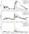 |
Fig. 6. Same as Fig. 5, but for WIND data at 0.99 AU. |
| In the text | |
|
Fig. 7. Magnetic field components in the RTN system, magnetic field strength and plasma properties of the ICME obtained from the model runs with different insertion directions, namely, P1 (blue), P2 (red), P3 (cyan), and P4 (orange) plotted on top of the observed in situ values (black) at the SolO heliocentric distance of 0.43 AU. |
| In the text | |
|
Fig. 8. Same as Fig. 7, but compared with in situ values at the WIND heliocentric distance of 0.99 AU. |
| In the text | |
|
Fig. 9. Bz component of the spheromak in HEEQ coordinates shown on (a) the equatorial plane and (b) the meridional plane. The coloured dots indicate the locations of the virtual spacecraft at 1 AU. Adjacent spacecraft are longitudinally separated by 5°. The central dot (cyan) denotes the location of Earth. |
| In the text | |
|
Fig. 10. Modelled magnetic field components in the GSE system, magnetic field strength and plasma properties, and the magnetic and plasma profiles (density and speed) obtained at the virtual spacecraft located within 10°E–10°W and 10° N–10° S at 1 AU plotted on top of WIND measurements. |
| In the text | |
|
Fig. 11. Magnetic field strength (top panel), density (middle), and speed (bottom panel) of the ICME obtained from the model runs using different magnetic flux inputs plotted on top of the observed in situ measurements at 0.43 AU. |
| In the text | |
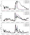 |
Fig. 12. Same as Fig. 11, but for comparison with in situ measurements at 0.99 AU. |
| In the text | |
|
Fig. 13. Comparison of the model results (model parameters in Table 5) with the in situ magnetic field components in the RTN system, magnetic field strength and plasma properties at 0.43 AU. The black solid curves denote the measurements from SolO, while the red solid curves are model outputs for the three components of the magnetic field (top three plots), the magnetic field strength (middle plot), and the plasma beta, number density and speed, respectively (bottom three plots). The vertical green dashed lines mark the estimated magnetic cloud boundaries, within which the plasma beta becomes less than 1 in the simulation results. |
| In the text | |
|
Fig. 14. Same as Fig. 13, but for WIND data at 0.99 AU. The blue solid lines in the top four plots are the same as the model output, indicated by the red solid lines, but shifted by 15 hours and 48 minutes so that the front edge of both the observed and modelled flux rope temporally coincides. |
| In the text | |
|
Fig. 15. CME magnetic field magnitude as a function of distance from 0.2 AU to 2 AU from final simulation results in log-log scale. The red line represents the least-squares power-law best fit. |
| In the text | |
|
Fig. 16. Magnetic field strength of the ICME obtained from the model runs using different magnetic flux inputs from our methodology, and PEA estimated flux plotted against the in situ measurements at 0.43 AU (top) and 0.99 AU (bottom). |
| In the text | |
Current usage metrics show cumulative count of Article Views (full-text article views including HTML views, PDF and ePub downloads, according to the available data) and Abstracts Views on Vision4Press platform.
Data correspond to usage on the plateform after 2015. The current usage metrics is available 48-96 hours after online publication and is updated daily on week days.
Initial download of the metrics may take a while.