| Issue |
A&A
Volume 706, February 2026
|
|
|---|---|---|
| Article Number | A348 | |
| Number of page(s) | 22 | |
| Section | Catalogs and data | |
| DOI | https://doi.org/10.1051/0004-6361/202556113 | |
| Published online | 25 February 2026 | |
The ANDICAM-SOFI Near-infrared and Optical type Ia Supernova (ASNOS) sample: Description and data release
1
Institut d’Estudis Espacials de Catalunya (IEEC),
08034
Barcelona,
Spain
2
Institute of Space Sciences (ICE, CSIC), Campus UAB,
Carrer de Can Magrans s/n,
08193
Barcelona,
Spain
3
School of Physics, Trinity College Dublin, The University of Dublin,
Dublin 2,
Ireland
4
Instituto de Ciencias Exactas y Naturales (ICEN), Universidad Arturo Prat,
Chile
5
Department of Physics and Astronomy, Aarhus University,
Ny Munkegade 120,
8000
Aarhus C,
Denmark
6
Observatories of the Carnegie Institution for Science,
813 Santa Barbara St, Pasadena,
CA 91101,
USA
7
Institute for Astronomy, University of Hawai ’i at Manoa,
2680 Woodlawn Drive, Hawai ’i, HI
96822,
USA
8
Oskar Klein Centre, Department of Physics, Stockholm University,
AlbaNova,
10691
Stockholm,
Sweden
9
European Southern Observatory,
Alonso de Crdova
3107,
Casilla 19 Santiago,
Chile
10
Institute for Astronomy, University of Hawaii,
2680 Woodlawn Dr., Honolulu, HI
96825,
USA
11
Astronomical Observatory, University of Warsaw,
Al. Ujazdowskie 4, 00-478
Warszawa,
Poland
12
Graduate Institute of Astronomy, National Central University,
300 Jhongda Road,
32001
Jhongli,
Taiwan
★ Corresponding author: This email address is being protected from spambots. You need JavaScript enabled to view it.
Received:
26
June
2025
Accepted:
27
November
2025
Abstract
Type Ia supernovae (SNe Ia) provide the robustest means of measuring extragalactic distances. While increasing the number of SNe Ia observed in the optical has received most effort so far, near-infrared (NIR) observations remain scarce despite their advantages. The dust extinction in NIR observations is lower and the behavior of standard candles is more intrinsic and therefore requires little to no empirical corrections. We present the ANDICAM-SOFI Near-infrared and Optical type Ia Supernova (ASNOS) dataset with sample size of 1482 epochs in the BVRIYJH filters from the ANDICAM instrument on the 1.3-meter SMARTS telescope at Cerro Tololo Inter-American Observatory, along with 125 JHK epochs from the SOFI instrument on the 3.58-meter New Technology Telescope on the La Silla Observatory. Additionally, we incorporate optical forced photometry from the Zwicky Transient Facility and the Asteroid Terrestrial-impact Last Alert System. The sample comprises 41 SNe Ia in total, including 29 normal events, eight 1991T-like objects, and four peculiar subtypes, all located at redshifts z<0.085. We provide a detailed overview of the ASNOS sample selection, data reduction, SN photometry, construction of the global and local host-galaxy spectral energy distribution, and SN light-curve fitting using three methods: SALT3-NIR, SNooPy, and BayeSN. A companion paper will present the cosmological analysis.
Key words: distance scale
© The Authors 2026
 Open Access article, published by EDP Sciences, under the terms of the Creative Commons Attribution License (https://creativecommons.org/licenses/by/4.0), which permits unrestricted use, distribution, and reproduction in any medium, provided the original work is properly cited.
This article is published in open access under the Subscribe to Open model. This email address is being protected from spambots. You need JavaScript enabled to view it. to support open access publication.
1 Introduction
Type Ia supernovae (SNe Ia) are thermonuclear explosions that occur in stellar systems with at least one white dwarf (WD). The WD is supported by electron degeneracy pressure, which counteracts gravitational collapse. Several progenitor scenarios have been proposed for SNe Ia, the most common of which is the single-degenerate scenario (Whelan & Iben 1973), which involves a WD and a main-sequence companion. The double-degenerate scenario (Webbink 1984) consists of two WDs. Configurations of triple systems (Thompson 2011) were also suggested, in which two WDs and a tertiary star can interact to induce a direct collision between the WDs (Kushnir et al. 2013). Another scenario are systems with WDs and post-asymptotic giant branch (pAGB) companions (Livio & Riess 2003; Kashi & Soker 2011). In each of these scenarios, the explosion might be triggered by either mass accretion from a companion or by stellar mergers. The explosion mechanisms include central or outer carbon ignition and ignition of the surface helium. These combination of progenitor scenarios and explosion mechanisms result in either near-Chandrasekhar-mass (MCh) or sub- MCh progenitor WDs that explode as SNe Ia (Hillebrandt & Niemeyer 2000). SNe Ia can reach a peak luminosity of about 1043 erg s−1, and their light curves are highly homogeneous, which makes them ideal for measuring cosmological distances. They have been used to demonstrate the accelerated expansion of the Universe (Perlmutter et al. 1999; Riess et al. 1998) and to measure the local expansion rate (e.g., Riess et al. 2022; Galbany et al. 2023).
In most cases, SNe Ia are observed at optical wavelengths, and more than 6000 observed objects are publicly available (Scolnic et al. 2022; Rigault et al. 2024; DES Collaboration 2024). The peak B-band brightness of SNe Ia correlates with the post-peak decline rate 15 days after maximum Δ m15 (Pskovskii 1977; Phillips 1993) and with the B−V color at peak (Riess et al. 1996; Tripp 1998). They can therefore be used as standardizable candles when stretch and color corrections have been applied. Analyses of SNe Ia in the near-infrared (NIR) have shown that they are nearly natural standard candles because the NIR light is less affected by dust and because their peak luminosities are less strongly scattered intrinsically (Krisciunas et al. 2004; Barone-Nugent et al. 2012; Stanishev et al. 2018; Jha et al. 2019; Müller-Bravo et al. 2022). Unfortunately, it is challenging to observe in the NIR because the sky background is brighter and the host galaxies are often brighter than the SNe, which hinders an accurate determination of their brightness. The largest publicly available samples of SNe Ia with NIR light curves include SNe Ia from the Carnegie Supernova Project (CSP-I: Contreras et al. 2010; Stritzinger et al. 2011; Krisciunas et al. 2017; CSP-II: Phillips et al. 2019; Hsiao et al. 2019), the Harvard Center for Astrophysics (CfA; Friedman et al. 2015), the RATIR sample (Johansson et al. 2021), SweetSpot (Weyant et al. 2018), RAISIN (Jones et al. 2022), DEHVILS (Peterson et al. 2023), and the Hawai’i Supernova Flows (Do et al. 2024). Ongoing projects such as Supernovae in the InfRAred Avec Hubble (SIRAH; Jha et al. in prep.; Galbany 2020) are expected to increase the sample size by a few dozen objects in the coming years. The total number of publicly available SNe Ia with NIR JH-band observations is currently about 300, which is significantly smaller than the number of publicly available objects at optical wavelengths.
Our aim is to expand the number of SNe observed in the NIR by presenting 41 SNe with optical (BVRI) and NIR (YJHKs) data obtained using the instrument called A Novel Dual Imaging CAMera (ANDICAM; DePoy et al. 2003) mounted on the 1.3-meter SMARTS telescope at the Cerro Tololo Inter-American Observatory (CTIO). The main goal is to provide an expanded sample of SNe Ia with NIR observations to enable precision cosmology.
Additionally, we included JHKs images taken with the instrument called Son OF ISAAC (SOFI), which is mounted on the 3.58-meter New Technology Telescope (NTT) at La Silla Observatory. We describe the methods we used to reduce the data and calculate the brightness of the SNe at various epochs to construct light curves. We then used the light-curve fitting tools SNooPy (Burns et al. 2014), BayeSN (Grayling et al. 2024), and SNCosmo (Barbary et al. 2025) with the SALT3-NIR template (Pierel et al. 2022) to fit our data and determine the light-curve parameters. Furthermore, global and local host galaxy parameters were obtained by performing photometry with Hostphot (Müller-Bravo & Galbany 2022) and conducting stellar population synthesis with Prospector (Leja et al. 2017; Johnson et al. 2021). This is the first of two papers and describes the data reduction and the release in general. The second paper will focus on studying Hubble diagram residuals using a combination of our data and other datasets that are available in the literature. The methods we applied here will serve as the basis for our project Aarhus-Barcelona cosmic FLOWS, in which we currently have more than 700 observations of SNe Ia in the NIR.
2 Data sample
2.1 Target selection and observing strategy
Our observing campaign lasted three semesters (2018A-2019A), during which the objective was to observe approximately 12 SNe per semester. To select targets for the observation, we monitored newly classified objects in the Transient Name Server (TNS1) and ensured that each object would be observable from CTIO for about two months at magnitudes brighter than 18 mag. Although our initial goal was to select nearby objects in the Hubble flow with redshifts between z=0.01 and 0.04 to accurately measure distances to their host galaxies, we included a few SNe at higher redshifts (but still within the Hubble flow). The objective was to obtain ten epochs in each band (JH) for each SN, covering a time span from −10 to +50 days past the optical peak, with observations approximately every six days. This cadence would allow us to determine the peak magnitude in JH and capture the behavior around the secondary peak in the NIR. Unfortunately, the optical camera malfunctioned in April 2019, which limited our ability to obtain optical images. As a result, the last five SNe in the sample only contained I-band images.
2.2 ANDICAM images
The images were obtained using the SMARTS telescope at CTIO with the ANDICAM camera, which had been in operation for approximately 20 years. Its last observation was taken in July 2019. We obtained simultaneous optical (BVRI) and NIR (YJH) images, with pixel scales of 0.371 and 0.271 arcsec/pixel and a field of view (FoV) of 6 × 6 and 2.4 × 2.4 arcmin2 for the optical and NIR channels, respectively. In total, 41 SNe were observed with ANDICAM, 29 of which were classified as normal SNe Ia, 8 as 1991T-like SN, 2 as 1991bg-like SN, 1 as SNe Ic-broad line, and one as a 2002cx-like SN. A total of 33 out of 41 SNe had Y-band images, and the median number of epochs in YJH was 12. The optical images were taken with an exposure time of 200 s, while the NIR images were acquired in sets of five at different dither positions by 10 or 20 arcsec, each with an exposure time of 20 s. Only one set of dithered images was obtained in the Y-band images, and two sets were taken for JH. A few K-band images were also obtained, but they were too noisy to be useful and were therefore excluded from this study. Additionally, we obtained images of standard stars on the same nights as our SN observations.
Table A.1 presents the list of SNe observed with ANDICAM, along with their subtypes, right ascensions (RA), declinations (Dec), discovery groups, classification groups, all obtained from TNS, which reports new astronomical transients such as supernova candidates. To match host galaxy and redshift, a thorough search was made in the NASA/IPAC Extragalactic Database (NED2), the SIMBAD astronomical database3 and in the second data release of the Zwicky Transient Facility (ZTF DR2; Rigault et al. 2025). In the last column, we also included the number of epochs in YJH.
2.3 Additional NIR SOFI images
Images taken with the SOFI instrument on the NTT in La Silla were obtained through the Public European Southern Observatory Spectroscopic Survey of Transient Objects (PESSTO) collaboration (Smartt et al. 2015) and typically consisted of one to five epochs of JHKs images. The pixel scale is 0.25 arcsec/pixel, and the images cover a FoV of 5 × 5 arcmin2. A summary of images collected with SOFI is also included in Table A.1.
2.4 Additional optical data
In addition to our optical ANDICAM images, we obtained optical data from the Asteroid Terrestrial-impact Last Alert System (ATLAS; Tonry et al. 2018) and the Zwicky Transient Facility (ZTF; Bellm et al. 2018). ATLAS is a highly efficient system for detecting potentially hazardous asteroids, as well as for tracking and discovering transients, with a two-day cadence in the cyan (c; 4200–6500 Å) and orange bands (o; 5600−8200 Å). Currently, ATLAS observes the whole sky with a cadence of one day between declinations of −50 and +50 and two days in the polar regions, weather permitting. The images were calibrated using the Pan-STARRS catalog (Chambers et al. 2019), and the light curves are publicly available through The ATLAS Project Fallingstar photometry service4. Optical data from the ZTF were retrieved from the ZTF second data release (Rigault et al. 2025) and were obtained using the Palomar 48-inch Schmidt telescope, which scanned the entire northern sky visible from Palomar every two days in the g(3676−5614 Å) and r band (5498–7394 Å), while alerts were distributed in real time to the brokers for the i band (6870–8964 Å).
2.5 Host-galaxy template images
When the SN occurred in a bright galaxy region, it was crucial to remove the underlying host-galaxy light contamination to precisely measure the SN brightness in the image. This was done by verifying that the background level around the SN was close to zero. Ideally, host-galaxy template images should be taken with the same instrument, but ANDICAM stopped operating immediately after our program ended in July 2019. As a result, we had to either rely on archival images or obtain new images with other facilities.
The NIR images were obtained through the European Southern Observatory (ESO) archive5 and The United Kingdom Infrared Telescope (UKIRT) Hemisphere Survey archive6. We also attempted to use 2MASS templates, but the resolution of these images was insufficient to provide a good subtraction. When no archival templates were available, new templates were obtained using the NOTCam camera at the 2.5-meter Nordic Optical Telescope (NOT) in La Palma or SOFI at the NTT in La Silla through the PESSTO collaboration. Furthermore, our project was awarded one night to observe at the 6.5-meter Magellan Baade telescope using the FourStar instrument (Persson et al. 2013) located on Las Campanas Observatory in Chile. Optical template images, on the other hand, were obtained from the Dark Energy Survey7 (DES), Pan-STARRS8, SkyMapper9, or EFOSC at NTT (again, through the PESSTO collaboration). When it was not possible to obtain BVRI templates for subtraction, we used g-band templates for B and V, r for R, and i instead of I in a few cases. Since all NIR template images were taken in 2023 or later, the SNe had long since faded because our SNe were observed in 2018–2019.
3 Data reduction
3.1 ANDICAM imaging
The optical ANDICAM images were directly retrieved from the SMARTS FTP archive and had already been reduced using the dedicated ANDICAM pipeline10, which applies bias and flat-field corrections to the images. The NIR images were provided in raw format, and we therefore describe the data reduction process here, including flat-field and dark corrections, sky subtraction, and the combination of dithered images.
3.1.1 Flat and dark correction
To reduce our ANDICAM NIR images and our standard stars, we used ccdproc11, an Astropy-affiliated package for the reduction of charge-coupled device (CCD) images. This allowed us to take an image in FITS format and convert it into a CCDData object, which is a matrix containing the photon counts at each pixel position in our images. Flats were already combined into master flats and made available in the SMARTS FTP archive. Individual dark frames taken during a night were combined into a master dark. To create the master dark for a given date, all dark images taken on that date were collected and CCDproc.combine was used to combine the dark frames entry-wise by taking the median. Because flats and darks were not taken every night, we selected the flat and dark images from the FTP archive that were closest in time to when the raw science images were taken (typically two to three days apart at worst). The master flat and master dark were used for the SN images and standard stars. The master dark was subtracted from each raw image using CCDPROC.SUBTRACT_DARK, which scales the master dark to match the exposure time of the raw image and then subtracts it. In our case, the exposure times were the same, and no scaling was therefore needed. Finally, ccdproc.flat_correct was used to normalize the master flat using the median of the matrix (if not already done), and then, the dark-subtracted images were divided by the flat entry-wise.
Figure 1 illustrates the process of dark and flat correction for a single raw image. We note an artifact in the middle right region of all our images that we were unable to remove entirely during the master flat correction. This artifact does not affect the SN magnitude, however, because the SN is consistently positioned near the center in all our images. For the Y-band images, no Y-band flats were available in the SMARTS FTP archive, and we therefore used a J-band flat instead. By comparing the differences between the J- and H-band flats, we found that the variation between them is lower than 2%, resulting in differences in the instrumental magnitudes of local sequence stars of 0.02 magnitudes in the worst cases (in either direction). As a result, an uncertainty to the instrumental magnitude in the Y band of 0.02 magnitudes was added in quadrature. Because an ∼ 2% offset in the Y-band photometry might arise from the use of J-band flats during the data reduction, we do not recommend using these data for precision cosmology and excluded them from our light-curve fitting.
3.1.2 Cosmic-ray removal
Cosmic rays were removed using the COSMICRAY_LACOSMIC module from CCDPROC, which detects and removes cosmic rays based on the readout noise, a sigma-detection threshold (which was set to the default value of 5), and the science image as input parameters. Panel F in Figure 1 shows the detected cosmic rays, and the image corrected for cosmic rays is shown in panel G.
3.1.3 Quadrant correction
In some science images, the background levels differ between quadrants, which is shown in panel G in Figure 1. To address this issue, the image was divided into four quadrants, and bright sources were masked out. The background level in each quadrant was then estimated and subtracted accordingly. The estimated background level for each quadrant is shown in panel H of Figure 1, while the science image corrected for quadrant features is shown in panel I. Before we subtracted the quadrant backgrounds, we estimated the overall background level of the full image and stored it for later use in rescaling the final science frame. Additionally, the background level was used to select images with the similar background levels to construct a sky background (see Sect. 3.1.4 for more details).
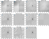 |
Fig. 1 Example of a raw image reduction for an ANDICAM J-band image. Top row (left to right): single raw image of SN 2019so, master dark, and dark-reduced raw image using the two previous images and a master flat. Middle row: flat and dark-reduced image, detected cosmic rays, cosmic-ray-corrected image, and quadrant background level. Bottom row: image corrected for quadrant features, sky image, and sky-subtracted image. The sky image was evaluated from the remaining set of dithered images taken on the same night. The host galaxy was masked out for each single image when we constructed the sky image. |
3.1.4 Sky subtraction
The next step was to remove the sky background, which can vary significantly in the NIR, even when images were taken just a few minutes apart. To achieve this, the following procedure for a set of dithered images was used: At a given epoch, the median and standard deviation of all images were evaluated. These values were saved to rescale the final science image afterward, ensuring that reliable uncertainties for the photometry were maintained. We estimated the standard deviation of the sky medians and called this value sky_std. Similarly, we estimated the average of the standard deviations and called this value sky_noise. When sky_std < sky_avg, some images had background levels that were different from the rest. These were excluded until sky_std > sky_avg. For a given image in a set of dithered images, we then used ccdproc.combine on the remaining images to create a sky background. Finally, the sky background was subtracted from each image. In some cases, a large object such as the host galaxy might be larger than the dithering step size, which might result in a brighter sky image around the location of the host galaxy. To address this issue, bright sources were masked out in each image before the images were combined into a single sky image.
Panel J of Figure 1 shows the sky image without the area around the host galaxy, and the final sky-subtracted image is shown in panel K. Here, it was possible to successfully capture and remove the wave-like structure in the sky background from the dark- and flat-corrected image.
3.1.5 World coordinate system
Only the NIR ANDICAM images lacked any world coordinate system (WCS) values in the image header. To obtain them, we used nova.Astronometry.net12, which requires at least three stars that can be detected by the code. This was difficult because the stars were faint and the FoV was quite small (2.4 × 2.4 arcmin2). For SN 2018hhn, SN 2018jag, and SN 2019cxx, we were unable to obtain a WCS. Therefore, these images were combined using the relative position of the host galaxy. This was succesful for SN 2018hhn and SN 2018jag, but we were unable to obtain any stars and galaxies in the images of SN 2019cxx.
3.1.6 Combined final images
The dithered images were then combined into a single science image. To do this, each image was projected onto a grid of NaNs based on the relative position of a star. From the list of grids, we used numpy.nanmedian to combine the images. Finally, the edges were cropped to ensure that the final image had at least 50% of the coadded images throughout.
3.2 Complementary imaging
As described above, we also obtained data from SOFI, ZTF, and ATLAS, which were used in the SN Ia template light-curve fitting process. The ZTF light-curves were retrieved from ZTF DR2 (Rigault et al. 2024). We describe the data reduction processes for each of the other datasets in detail below.
3.2.1 SOFI
The raw SOFI NIR sciences images, flats, and darks were downloaded from the ESO archive13 and reduced using the PESSTO pipeline14. This pipeline handles the flat and dark corrections of the raw science images and the sky subtraction and individual frame combination.
3.2.2 ATLAS
The ATLAS data were obtained through the ATLAS forced photometry homepage. We requested epochs between −50 to +100 days of the detection date of the SN to ensure that the LC peak(s) were obtained. ATLAS often took four measurements per night, so that the data were stacked following The ATLAS Project’s Python plotting software (Young 2020). The fluxes and errors in the output file were given in microJansky, denoted μJy and dμJy, respectively. The fluxes were converted into AB magnitudes using
 (1)
For the magnitude error, the homepage suggested a Taylor expansion of log10(μJy ± dμJy) when d μJy/μJy was small, but since this was not always the case, we chose to propagate the error instead, where we set
(1)
For the magnitude error, the homepage suggested a Taylor expansion of log10(μJy ± dμJy) when d μJy/μJy was small, but since this was not always the case, we chose to propagate the error instead, where we set
 (2)
Nondetections were removed using a 3 σ upper limit,
(2)
Nondetections were removed using a 3 σ upper limit,
 (3)
(3)
In general, no baseline correction was required for ATLAS photometry. In two epochs, however, ATLAS changed the reference images, and therefore, the baselines changed. For SN 2018bie and SN 2018exc, we observed that the flux values of nondetections before and after the SN light curve significantly deviated from zero (∼−600 in flux space). Notably, at about 400 days post-explosion, these nondetections returned to zero flux. Without a baseline correction, the apparent magnitudes appeared to be artificially faint. To account for this, a baseline correction was implemented exclusively for these two SNe. The baseline level was determined using a trimmed mean of the flux values from epochs earlier than −30 days and later than +400 days relative to the SN detection date to ensure that any residual supernova signal was excluded. When we fit the light curve (see Sect. 5), the resulting fits were significantly improved with the baseline correction, and the fits were poor without a correction.
3.3 Background subtraction
The background was finally subtracted from the optical ANDICAM images and SOFI images (this was already done for the NIR ANDICAM images). The background was subtracted using Background2D from photutils.background. Here, we used MedianBackground, which calculated the background in an array as the sigma-clipped median, with sigma set to 3. Figure 2 shows an example of the background subtraction. All reduced images can be accessed from GitHub15.
4 Photometry
We describe the methods we used to determine the apparent magnitudes of our SNe and to construct the light curves. This process includes template subtraction, aperture photometry, calculating zeropoints, and determining the color term coefficients. The color term coefficients quantify the difference of a natural system from the standard system as a function of the color of an object, and it allowed us to transform magnitudes from one system to the other. A natural system refers to the photometric system native to the telescope and detector setup, or in other words, the system response function, and a standard system refers to a widely used photometric system such as the Johnson system. The objective was to construct SN light curves in the natural system.
4.1 Template subtraction
Before our images were used for photometry, the light from the host galaxy was removed using the software ImageMatch16. This software rectifies an image by matching point-sources from the science image to the host-galaxy template and by solving for a geometric transformation from one to the other. Afterward, the software convolved one image with a seeing kernel that blurred it, so that the images matched in resolution, which resulted in clean subtractions. The seeing in the science image was better than the template in only a few cases, and the science image therefore needed to be blurred so that it matched the template for a proper subtraction. By default, ImageMatch performs the subtraction over the entire image. For photometric measurements, a small region centered on the SN from the subtracted image was instead inserted into the original unsubtracted frame containing all field stars. This procedure allowed the apparent SN magnitude to be estimated in a single step: first determining the zeropoint from local sequence stars, and then measuring the instrumental SN magnitude. To assess the quality of the subtraction, the entire subtracted image was visually inspected to confirm that nearby stars and galaxies were properly removed.
Figure 3 shows an image before and after subtraction. The light from the host galaxy was clearly subtracted around the SN. For a few cases, a proper subtraction when the SN was at the center of the host was not possible. This was likely because templates and science images were from other instruments/filters. This was the case for SNe 2018dda, 2018exb, 2018exc, and 2018feq. Light-curve fits were attempted for these SNe, but the fits were poor and the SN was not clearly isolated. We therefore did not use these images.
To confirm the effect of our template subtractions, we compared the apparent magnitude of various SNe with and without subtraction based on their distance from the host. This was accomplished using the angular distance to the SN normalized by the directional light radius of the host galaxy, denoted dDLR (Sullivan et al. 2006; Gupta et al. 2016; Sako et al. 2018), and it depends on the shape of the galaxy and the SN direction. Generally, dDLR<1 means that the SN is inside the ellipse of the host galaxy, while dDLR>1 means that it is outside and therefore would be very little affected by the light of its host. Hence, SNe with dDLR>1 were used as a consistency check to determine whether our subtractions were effective. The software SEP17 was used to determine the shape of the host galaxy. SEP is a Python implementation of Source Extractor18 and determines the sizes and shapes of stars/galaxies in an image in terms of elliptical parameters such as semimajor and semiminor axis. Figure 4 shows an example of the evaluation of dDLR for a host galaxy with its shape (in orange) determined from SEP using a 3 σ detection threshold. Table A.1 shows dDLR for all SN hosts in our sample. In each case, r-band images were used (mostly from Pan-STARRS, SDSS, and DES). The results of estimating dDLR for a few SNe are shown in Figure 5. The top panels show the apparent magnitude of some SNe with different dDLR with subtraction (filled circles) versus no subtraction (empty circles) for the ANDICAM BVRI. The bottom panels show the corresponding histograms of the apparent magnitude difference between nonsubtracted and template-subtracted images, where the median difference is presented in the legend. The subtracted and nonsubtracted images did not differ strongly, as expected, when the SN was far away from its host, but the contamination from the host was significant when the SN was close.
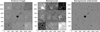 |
Fig. 2 Example of the background subtraction for a SOFI image. Left: combined J-band science image of SN 2018agk taken with SOFI. Middle: detected image background using photutils.BACKGROUND2D. Right: background- and cosmic-ray subtracted image. We were able to remove most of the quadrant structure from the image. |
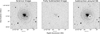 |
Fig. 3 Template subtraction using ImageMatch. Left: science image without template subtraction. Middle: fully subtracted science image. Right: template-subtracted image using ImageMatch with the SN in the middle of the subtracted area. ImageMatch does subtraction on the full image, but one can choose to have the subtracted area around the SN inserted back into the original science image. |
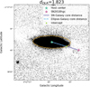 |
Fig. 4 Example of measuring dDLR. The shape of the host was measured using sep and is plotted in orange. The dDLR is the ratio of the distance from the host center to the SN (purple) and the distance from the host center to the edge of the ellipse (dashed blue). |
4.2 Absolute photometry
To evaluate the brightness of the local sequence stars and the SN in our images, we used the package photutils19. With DAOStarFinder, sources in our images that were 3 σ above background level were detected. Each source was then fit with 2D Gaussian to determine their geometric properties such as position, semimajor axis, semiminor axis, and full width at half maximum (FWHM), which is the width of the distribution measured between two points, where the value of the curve is at half its maximum amplitude. The world coordinate system (WCS) in the image header was used to assign catalog magnitudes to each object when the relative distance between the position obtained from DAOStarFinder and the catalog position was shorter than 0.5 FWHM.
4.2.1 Reference catalog
The ATLAS-REFCAT2 catalog (Tonry et al. 2018), an allsky reference catalog containing about one billion stars down to an apparent magnitude of 19, was used to assign catalog magnitudes to our sources. REFCAT2 consists of a variety of surveys such as PanSTARRS, The AAVSO Photometric AllSky Survey (APASS), SkyMapper, and the Two Micron All Sky Survey (2MASS). The PanSTARRS magnitudes (gri) from ATLAS-REFCAT2 were transformed into Johnson BVRI, which corresponded to the optical passbands of ANDICAM, using the transformations in Tonry et al. (2012),
 (4)
where the subscript p denotes Pan-STARRS passbands, and the subscript cat,std denotes the catalog magnitude in a standard photometric system such as the Johnson system. The ANDICAM Y passband was similar to the Dark Energy Camera (DECam) Y passband, so that our catalog magnitudes had to be transformed into DECam magnitudes. The color-term coefficients would be determined later on, and we therefore evaluated DECam z-band magnitudes as well in order to have a filter that was close to the Y band in terms of wavelength range. This required Pan-STARRS zy bands, but since the ATLAS-REFCAT2 only had PanSTARRS griz, we used the 2MASS transformations from Tonry et al. (2012) to obtain the PanSTARRS y band,
(4)
where the subscript p denotes Pan-STARRS passbands, and the subscript cat,std denotes the catalog magnitude in a standard photometric system such as the Johnson system. The ANDICAM Y passband was similar to the Dark Energy Camera (DECam) Y passband, so that our catalog magnitudes had to be transformed into DECam magnitudes. The color-term coefficients would be determined later on, and we therefore evaluated DECam z-band magnitudes as well in order to have a filter that was close to the Y band in terms of wavelength range. This required Pan-STARRS zy bands, but since the ATLAS-REFCAT2 only had PanSTARRS griz, we used the 2MASS transformations from Tonry et al. (2012) to obtain the PanSTARRS y band,
 (5)
where the subscript 2 denotes 2MASS magnitudes. Finally, the transformations from Abbott et al. (2021) were used to obtain DECam zY magnitudes,
(5)
where the subscript 2 denotes 2MASS magnitudes. Finally, the transformations from Abbott et al. (2021) were used to obtain DECam zY magnitudes,
 (6)
(6)
Before we determined the instrumental magnitude of our sources, a few cuts were applied: 1) Objects that were 3 • FWHM from the edges of our images were removed (our images consisted of multiple dithered images, and therefore, stars closer to the edge had fewer images than those in the center, which therefore gave less precise measurements). 2) Galaxies were removed. 3) Saturated objectives were removed. This was achieved by calculating the maximum pixel value for each source and removing objects for which the detector limit was exceeded and the detectors would become nonlinear. For ANDICAM optical, ANDICAM NIR, and SOFI, the limits were 45 000, 5000, and 10 000 ADU, respectively.
4.2.2 Instrumental magnitude
To determine the natural instrumental magnitudes of our sources, we used Circular_Aperture from photutils.aperture, which evaluated the total counts within a circle of a given radius. For each image, a 3 σ clipped median of the distribution of FWHM of our local sequence stars was evaluated. The aperture radius of all our sources (including the SN) was then set to be 0.6731 times the median FWHM, which is the optimum aperture size for photometry of sources whose profiles can be approximated as Gaussian20. An example of this procedure is shown in Figure 6.
To convert the counts inside the apertures into instrumental magnitudes in the natural system minst,nat (i.e., the magnitude system measured by the telescope), we used
 (7)
where texposure is the total exposure time divided by the number of coadds (for ANDICAM NIR, this was just the exposure time of a single image because the coadded images were divided by the mask). To correct for extinction, for instance, for the B band, we used the equation
(7)
where texposure is the total exposure time divided by the number of coadds (for ANDICAM NIR, this was just the exposure time of a single image because the coadded images were divided by the mask). To correct for extinction, for instance, for the B band, we used the equation
 (8)
Here, kB is the extinction coefficient, X is the air-mass value and was taken from the image header, and Binst,nat is the natural instrumental magnitude from Eq. (7). Table 1 in Stritzinger et al. (2005) was used to correct the ANDICAM BVRIY passbands for extinction from the central wavelength of each filter. The estimated extinction coefficients are shown in Table 1. The authors evaluated extinction coefficients at CTIO out to 11 000 Å, and the value at this wavelength was 0.003. Because this value is low, extinction corrections to the ANDICAM JH filters were not applied. Likewise,the La Silla Observatory homepage21 only lists extinction coefficients out to 9000 Å, and the value at this wavelength was 0.01. Therefore, the extinction coefficients in JHKs were assumed to be zero.
(8)
Here, kB is the extinction coefficient, X is the air-mass value and was taken from the image header, and Binst,nat is the natural instrumental magnitude from Eq. (7). Table 1 in Stritzinger et al. (2005) was used to correct the ANDICAM BVRIY passbands for extinction from the central wavelength of each filter. The estimated extinction coefficients are shown in Table 1. The authors evaluated extinction coefficients at CTIO out to 11 000 Å, and the value at this wavelength was 0.003. Because this value is low, extinction corrections to the ANDICAM JH filters were not applied. Likewise,the La Silla Observatory homepage21 only lists extinction coefficients out to 9000 Å, and the value at this wavelength was 0.01. Therefore, the extinction coefficients in JHKs were assumed to be zero.
 |
Fig. 5 Top panels: comparison of photometry using subtracted images (filled circles) vs. not using templates (empty circles) for SNe with different dDLR. Bottom: histogram of the apparent magnitude difference between subtracted and nonsubtracted images. The median value is reported in the legend for each filter. |
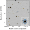 |
Fig. 6 Aperture radii (orange for the local sequence and blue for a supernova) for one of our science images. The inset at the bottom right is a zoom-in of the SN and its aperture. |
4.3 Image zeropoints
The method we used to evaluate the zeropoint for the science images is described below.
4.3.1 ANDICAM optical and SOFI
After the cuts described in the previous section, we determined the zeropoint from a sigma clipping using Chauvenet’s criterion. A linear function with a slope of unity in the form of f(x)=x+b was fit, where the zeropoint is the intercept in the instrumental versus catalog magnitude plot, where for a given star the instrumental magnitude is given by Eq. (8). Figure 7 shows an example of evaluating the image zeropoint, where sigma clipping was used to remove outliers. The error was set to be the weighted mean of the residuals between the fit and the data. The zeropoints we estimated were not the final zeropoint; they were only used to determine the color-term coefficients through an iterative process.
More generally, the y-axis in Figure 7 is the B-band instrumental magnitude in the ANDICAM natural system Binst,nat, while the x-axis is Bcat,std−CTB · (B−V)cat,std, where the subscript cat,std denotes a catalog magnitude in the Johnson standard system, and CTB is the B-band color term. Initially, the color term was unknown, and the x-axis in this case was Bcat,std. The idea was to use the initial image zeropoint to estimate an initial color term. With the initial color term, a new image zeropoint was estimated from the Bcat,std−CTB · (B−V)cat,std versus Binst,nat plot, which in turn would yield a new color term, and so forth. This iterative process is described in greater detail in Sect. 4.4.
Color-term coefficients for all filters using Emcee along with extinction coefficients.
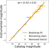 |
Fig. 7 Example of calculating an image zeropoint using bootstrapping with sigma clipping as outlier rejection, where the standard deviation from Chauvenet’s criteria was used. At the top of the panel, we show the image zeropoint and its error, the black line shows the fit using a linear function in the form of f(x)=x+b, the orange points represent the stars that remained after the sigma clipping, and the blue point(s) show rejected stars. The zeropoint is the intercept value from the fit. |
4.3.2 ANDICAM NIR
We evaluated the zeropoints of our standard field observations by plotting them as a function of observation date, as shown for the J band in Fig. 8. Even though standards were observed in the same nights, the zeropoints differed sometimes by half a magnitude, which should not be the case. This issue was also reported by Wang et al. (2020), who found differences in the nightly zeropoints of NIR standards using ANDICAM. They therefore used field stars with magnitudes in the 2MASS catalog. Attempts to apply color-term coefficients did not significantly improve the calibration. Consequently, these standard star fields were not used, and we instead adopted local sequence stars with catalog magnitudes from REFCAT2 to determine the image zeropoint.
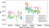 |
Fig. 8 J-band zeropoints for different nights. The zeropoints were computed using Jinst−J2, where Jinst is the instrumental magnitude evaluated from aperture photometry, and J2 is the 2MASS catalog magnitude in the J band. Standards taken in the same night give different zeropoints, which makes the standards too uncertain. |
4.4 Color-term coefficients
Ideally, color-term coefficients should be determined for each field of view in a given night, but the limited number of local sequence stars in most images prevented this. We instead combined stars observed at all epochs. To determine the color-term coefficients, for example, for the B band, the quantity Bcat,std− Binst,cor−ZPB, img was plotted against (B−V)cat,std for all B band images, and the slope of the relation was determined. Here, ZPB, img is the image zeropoint, which was determined following the procedure in Sect. 4.3.1.
For a given star observed at various epochs, a 3 σ clipping was made to remove outliers, and when the residuals were greater than 0.5 mag for a given star, the star was rejected. We thus also excluded potential variable stars. Additionally, we only selected stars whose uncertainties in instrumental magnitudes were smaller than 0.05 mag. The slope of the Bcat,std−Binst,cor− ZPB, img versus (B−V)cat plot was determined using a Markov chain Monte Carlo (MCMC) method with the Emcee package22.
The fitted slope to these data only provided an approximate color-term coefficient because the ZPB, img obtained in the previous step that was used to assemble the data from all nights into the same scale did not include any color-term correction. Therefore, an iterative approach was taken, in which we recomputed the zeropoint using the catalog magnitudes corrected for the newly computed color terms. Subsequently, the new zeropoint value ZPB,img,i was used to obtain a new color-term coefficient CTB, i. This process was iterated until the color-term value converged to four significant digits. This iterative process was essential because the zeropoint and color-term coefficients were interdependent and were only solved by a cyclic computation of the coefficients. More specifically, CTB, i, was used to colorcorrect the catalog magnitude as Bcat,std−CTB, i ·(B−V)cat,std, and a new image zeropoint, ZPB,img,i, was then evaluated in the same manner as in Fig. 7 from the Binst,nat versus Bcat,std−CTB, i. (B−V)cat, std plot. All B-band images were then used to determine a new slope from the Bcat,std−Binst,cor−ZPB,img,i versus (B−V)cat,std plot. The iterations continued until the slope value converged to four significant figures, which typically occurred after five iterations. Figure 9 shows the results of the Emcee fit for the final iteration (green) along with the slope determined from a least-squares fit in Scipy23 (orange). It shows that the Scipy and Emcee results agree. The mean and standard deviation were estimated for multiple color bins, and stars with extreme colors were excluded when the binned mean value was a 1 σ outlier from the fit relation.
Table 1 shows the estimated color-term coefficients for ANDICAM and SOFI, and Fig. F.1 in the appendix shows the corresponding fit for each filter. We realized that the color-term coefficient for Y was quite large, which was likely due to a small number of local sequence stars and the narrow color range. For Ks, the color term was large, but the error was only around 5%, which suggested that the SOFI Ks filter was different from the 2MASS Ks. After the color-term coefficients were evaluated, it was possible to evaluate the SN magnitude in the natural system. First, the catalog magnitudes of the local sequence stars in the standard system were transformed into the natural system. The relation between natural and standard magnitudes for the B band is
 (9)
where CTB is the B-band color-term coefficient. The newly obtained natural catalog magnitudes were then used to evaluate the natural image zeropoint ZPimg,nat using the same procedure as in Sect. 4.3.1, the only difference being that the catalog magnitude was transformed into the ANDICAM natural system, and the instrumental magnitudes were in the natural system and not corrected for extinction. With the natural image zeropoint, the apparent magnitude of the SN in the natural system was obtained following
(9)
where CTB is the B-band color-term coefficient. The newly obtained natural catalog magnitudes were then used to evaluate the natural image zeropoint ZPimg,nat using the same procedure as in Sect. 4.3.1, the only difference being that the catalog magnitude was transformed into the ANDICAM natural system, and the instrumental magnitudes were in the natural system and not corrected for extinction. With the natural image zeropoint, the apparent magnitude of the SN in the natural system was obtained following
 (10)
where mSN,nat is the instrumental magnitude of the SN. No extinction correction was applied to the local sequence stars/SN because they were observed in the same small FoV and therefore had the same airmass and extinction.
(10)
where mSN,nat is the instrumental magnitude of the SN. No extinction correction was applied to the local sequence stars/SN because they were observed in the same small FoV and therefore had the same airmass and extinction.
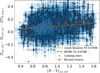 |
Fig. 9 Sigma-clipped Bcat,std−Binst−ZPB,img,i vs. (B−V)cat,std for all B band images in the sample (black). We estimated binned means (red) and their uncertainties and removed very red/blue stars when the bins did not agree with the fit. The legend gives the slope using Scipy least squares (orange) and the MCMC fitting code Emcee (green), which shows that the values agree. |
5 Light-curve fitting
We describe the light-curve fitting techniques SALT3-NIR, SNooPy, and BayeSN that we used to fit our light curves. For all three cases, we used a flat ΛCDM universe with Ωm0=0.3 and H0=70 km s−1 Mpc−1. Furthermore, the dust maps from Schlegel et al. (1998) were used to obtain the Milky Way color excess, and the reddening laws from Cardelli et al. (1989) were used to determine the Milky Way extinction for SNooPy, SALT3, and (Fitzpatrick 1999) for BayeSN (the Cardelli extinction law would have been used for BayeSN if it were possible, but this was not the case).
5.1 SALT3-NIR
SNCosmo24 is a Python library for the analysis of supernova cosmology. To fit the light curve in SNCosmo, we used the SALT3-NIR model (Pierel et al. 2022), which is an extension of the SALT3 model (Kenworthy et al. 2021). SALT3-NIR was trained on ∼ 1000 SN Ia with data at optical wavelengths and with 166 objects with NIR light curves. Additionally, SALT3-NIR was also trained with optical and NIR spectra to perform K-corrections. The output parameters included the amplitude x0, which is related to the B-band peak magnitude (Bmax ∼ −2.5 · log 10(x0)), the time of maximum t0, the stretch x1, which is related the shape of the LC, and the color c, which describes the supernova color (due to dust extinction or intrinsic properties). The model only reaches 20 000 Å, however, and we therefore did not include Ks-band images from SOFI.
We were unable to combine ATLAS data with our optical ANDICAM data in the optical wavelengths; in some cases, fitting ATLAS alone or ANDICAM alone provided succesful fits, but when we combined the two, the B-band fit was overestimated by 0.2–0.3 magnitudes with respect to the data. This was not the case for SNooPy and BayeSN. The same problems occurred for the SALT2 template. We searched the literature to determine whether some of our objects were observed by other telescopes. SN 2018aoz was studied by Ni et al. (2022) (see their supplementary Figure 3) and included B-band light curves with three different instruments (Korea Microlensing Telescope Network, KMTNet; Las Cumbres Observatory; and Swift Observatory).
The SN peaked with an apparent magnitude of Bmax=12.43 ± 0.08 mag (corrected for Milky Way extinction), which agrees with our results of 12.47 ± 0.07, while ATLAS-only data predicted that the SN peaked at 12.7 mag. Because our data agreed with three other observatories, we chose to exclude the ATLAS data whenever ANDICAM and ATLAS were incompatible.
Figure E.1 shows an example of light-curve fitting using SALT3-NIR along with BayeSN and SNooPy. From the output, we used source_peakmag to determine the peak BJH-band apparent magnitudes corrected for Milky Way extinction.
5.2 SNooPy
SNooPy (Burns et al. 2014) is a Python-based tool for modeling and analyzing Type Ia supernova photometry, calibrated using high-quality CSP light curves and templates in the uBVgriYJH filters. SNooPy has two different parameterizations for the shape of the light curves: Δ m15, which is the average decline 15 days after peak brightness when fitting all bandpasses, and the colorstretch parameter sBV (Burns et al. 2015), which measures the timing of the B−V peak with respect to the average time of 30 days past B-band maximum. For the light-curve fitting, we used the MAX_MODEL, which fits the maximum magnitude for each filter individually and performs K corrections and corrects for the Milky Way extinction. The fit model is of the form
 (11)
where TY is the light-curve template, mX is the observed magnitude in filter X, t′ is the de-redshifted time relative to B-maximum, Δ m15 is the decline rate parameter, mY is the peak magnitude in filter Y, RX is the total-to-selective absorption for filter X, and KXY is the cross-band K correction from rest-frame X to the observed filter Y. The output from using MAX_MODEL gives multiple maxima transformed into the CSP filter systems along with the time of maxima and sBV or Δ m15.
(11)
where TY is the light-curve template, mX is the observed magnitude in filter X, t′ is the de-redshifted time relative to B-maximum, Δ m15 is the decline rate parameter, mY is the peak magnitude in filter Y, RX is the total-to-selective absorption for filter X, and KXY is the cross-band K correction from rest-frame X to the observed filter Y. The output from using MAX_MODEL gives multiple maxima transformed into the CSP filter systems along with the time of maxima and sBV or Δ m15.
For the ANDICAM I-band photometry, we realized that SNooPy had a tendency to overestimate the secondary peak for most of our SNe while underestimating the first peak. This issue was also reported by Wee et al. (2018), who also found this trend in the light curve of SN 2017cbv, a nearby object (z ∼ 0.004). Since the I-band light curves were still able to reduce the uncertainties in the fitted LC parameters, the I-band light curves were still included.
5.3 BayeSN
BayeSN25 (Mandel et al. 2021; Grayling et al. 2024) is a hierarchical Bayesian model for SNe Ia SEDs that is continuous over time and wavelength. It ranges from the optical to the NIR, and the SED is modeled as a combination of distinct host galaxy dust and intrinsic spectral components. We used the Ward et al. (2023) model, which was trained on the Foundation DR1 compilation (Foley et al. 2017; Jones et al. 2019) and with Avelino et al. (2019) in the NIR. The training data included BgVrizYJH filters, which range from 3000 to 18 500 Å. The input parameters were the time of observation, the flux/magnitude, the flux error/magnitude error, a Milky Way color excess, and the redshift. The output of BayeSN gives a global distance modulus and the time of peak maximum along with their errors. From the fits, we obtained the peak magnitudes in each band (not corrected for extinction). The fitting results using the three fitters are reported in Table C.1 of the appendix. Figure 12 shows the difference in Bmax for the three light-curve fitters. BayeSN gives brighter Bmax than SNooPy, with most points lying above zero, whereas the SNe for SNooPy versus SALT are more evenly distributed around zero, and the same is true for BayeSN versus SALT. Our final SN light curves are shown in Appendix D along with the ZTF and ATLAS photometry.
6 Host galaxy masses
It was shown that the optical brightness of SNe Ia and the host mass of the SN are correlated (Kelly et al. 2010; Sullivan et al. 2010; Lampeitl et al. 2010), where SNe found in massive galaxies were intrinsically brighter after standardization than SNe in lowmass galaxies. To obtain more accurate distance measurements of the SNe, it is therefore important to take this mass step into account. In this section, we determine the host galaxy masses for our SNe.
6.1 Host galaxy photometry
Low-resolution spectral energy distributions (SEDs) of the host galaxies at various wavelengths were constructed using the Python package HostPHOt26 (Müller-Bravo & Galbany 2022). Only using the SN redshift and the host galaxy coordinates, HosPhot downloads images in various filters from several surveys archives, such as GALEX, Pan-STARRS, DES, 2MASS, and unWISE. We then calculated the global apparent magnitude of the host and at the local environment of the SN within a certain physical aperture (e.g., a diameter of 2 kpc using a flat LambdaCDM cosmology with a Hubble constant of H0=70 km s−1 Mpc−1 and a matter density parameter Ωm 0=0.3 as default) in all these filters. Before we computed the photometry, nearby foreground stars were masked out, which would otherwise cause the brightness of the galaxy to be overestimated. An example of this masking is shown in Figure 10. We defined elliptical apertures and computed global host galaxy photometry for all SNe in our sample and also local aperture photometry at 1, 2, and 3 kpc centered at the SN location.
6.2 Host galaxy properties
Prospector (Leja et al. 2017; Johnson et al. 2021) is a Python module for inferring stellar population parameters from photometry and spectroscopy. It ranges from the ultraviolet to infrared wavelengths. It is based on forward-modeling the data (i.e., predicting observational data by creating a theoretical model based on known physical principles) and Monte Carlo sampling of the posterior parameter distribution, which enables complex models and exploring moderate dimensional parameter spaces. Furthermore, Prospector uses the FSPS code (Conroy et al. 2009; Conroy & Gunn 2010), which allowed us to derive spectra of stellar populations. Emcee was used to obtain the posterior distributions of our host parameters, and for the star formation history (SFH), we used a nonparametric SFH that divided the galaxy lifetime into a series of time bins and estimated the star formation rate (SFR) in each bin independently. More specifically, we chose the continuity SFH, which, as described by Leja et al. (2019), allowed us to obtain a piecewise constant SFH without any sharp transitions in the SFH as a function of time. In order to obtain recent values in SFH, the first two bins were fixed between 0−30 Myr and 30−100 Myr, and the oldest time bin was fixed to 0.9 tuniv, where tuniv is the age of the Universe (we assumed a flat Λ CDM universe with Ωm0=0.3 and H0=70 km/s/Mpc, which is the same as for the light-curve fitters) at a given observed redshift. The remaining bins were equally spaced in time logarithmically between 100 Myr and 0.9 tuniv. Finally, the initial mass function from Kroupa (2002) was used, which is a broken power law with an exponent of −0.3 for 0.01< m/M⊙<0.08, −1.3 for 0.08<m/M⊙<0.5, and −2.3 at 0.5<m/M⊙<100. To run Prospector, we needed the galaxy SEDs from HostPhot and the redshift (held fixed). To avoid overfitting and reduce the computing time, only one filter for each wavelength regime was used (in other words, only one r band was selected when multiple r-band filters were available). For the optical regime, we therefore prioritized, based on how deep the surveys went and the number of filters, DES, SDSS, PanSTARRS, Legacy Survey, and SkyMapper, in this order. When the galaxy was too faint and resulted in negative fluxes (but consistent with zero), the flux was set to zero and the uncertainty to the 1 σ upper limit, as suggested in the Prospector documentation27. For the NIR data, the prioritization was UKIDSS, VISTA, and 2MASS. Finally, for the mid-infrared data from unWISE, only the W1 (λmean = 33 526 Å) and W2 (λmean=46 028 Å) filters were used because the image resolution in the far-infrared was usually very low. Figure 11 shows an example of the SED fitting using Prospector for the host galaxy of SN 2018ayg, LEDA 1573011. The global photometry from HostPhot and the Prospector parameters are listed in Table B.1, and the local photometry is listed in Table B.2.
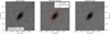 |
Fig. 10 Example of masking out stars using HostPhot. Left: initial image downloaded from Pan-STARRS. Middle: objects detected in HostPhot along with their apertures. Right: image without sources. |
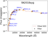 |
Fig. 11 Example of the SED fitting in Prospector. The black points show the flux (in maggies, where 1 maggie is equal to 3631 Jy) for our survey images. The fit SED profile is marked in brown, and the yellow boxes indicate the model value for a given survey. This is the initially detected aperture, not the final aperture measured by HostPhot. |
7 Summary and conclusion
We presented SMARTS-ANDICAM optical and NIR data for 41 SNe, complemented by NTT-SOFI NIR imaging. We described the data reduction and analysis procedures in detail. Far fewer NIR observations of SNe are publicly available (∼300) than observations in the optical (∼6000). The ASNOS sample increases the current NIR SN Ia dataset by approximately 10%.
The photometry of the ANDICAM NIR images could have been significantly improved if our standard stars had been more consistent with one another when observed in the same night. As demonstrated by Figure 8, this was not the case. We instead relied on faint local sequence stars within a limited field of view (FoV) of only 2.4 × 2.4 arcmin, and only three to four stars were available to determine the image zeropoint using the catalog magnitudes from ATLAS-REFCAT2. Ideally, template images for subtraction would have been taken with the same instrument after the SN had faded. Because the ANDICAM instrument was decommissioned in 2019, however, this was not possible. Additionally, the SOFI instrument ceased operation around 2023, just as our plan was to acquire template images. Archival data from different instruments therefore had to be used instead. We also observed differences in the color-term determinations from broadband photometry as compared to synthetic photometry computed using the CALSPEC spectrophotometric standards. Because the color-term coefficients remained small in both cases, however, the effect on the apparent magnitudes of the SNe is very weak.
The resulting light curves were fit using the three most widely used methods: SNCosmo with the SALT3-NIR template, SNooPy, and BayeSN. Finally, HOSTPHOT was used to derive spectral energy distributions (SEDs) of the host galaxies and local environments, and we employed Prospector to perform a stellar population synthesis and estimate the key galaxy parameters. After applying standard light-curve selection cuts, we retained a final sample of approximately 20 SNe with NIR observations. This first paper describes the data reduction process and a data release and reports all light-curve parameters and host galaxy masses. In a subsequent paper, we will combine literature SNe with our ANDICAM sample to measure extragalactic SN distances, construct Hubble diagrams, analyze the differences between optical and NIR observations, and explore the correlations between NIR Hubble residuals and host galaxy properties using various techniques such as host galaxy mass and specific star formation rate.
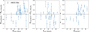 |
Fig. 12 Comparison of Bmax estimates from BayeSN, SALT3-NIR, and SNooPy. |
Data availability
The photometry catalogs are available at the CDS via https://cdsarc.cds.unistra.fr/viz-bin/cat/J/A+A/706/A348.
Acknowledgements
The SNICE group acknowledges financial support from the Spanish Ministerio de Ciencia e Innovación (MCIN) and the Agencia Estatal de Investigación (AEI) 10.13039/501100011033 under the PID2020-115253GAI00 HOSTFLOWS and the PID2023-151307NB-I00 SNNEXT projects, from Centro Superior de Investigaciones Científicas (CSIC) under projects PIE 20215AT016, ILINK23001, and the program Unidad de Excelencia María de Maeztu CEX2020-001058-M, and from the Departament de Recerca i Universitats de la Generalitat de Catalunya through the 2021-SGR-01270 grant. We acknowledge the financial support from the María de Maeztu Thematic Core at ICE-CSIC. S. Bose, M.D. Stritzinger, C. Soerensen, and the Aarhus-Barcelona FLOWS project are funded by the Independent Research Fund Denmark (IRFD, grant number 10.46540/2032-00022B) and by an Aarhus University Research Foundation Nova project (AUFF-E-2023-9-28). This research has used data from the SMARTS 1.3-m telescope, which is operated as part of the SMARTS Consortium. Based on observations at NSF Cerro Tololo Inter-American Observatory, NSF NOIRLab (NOIRLab Prop. ID NOAO-18A-0047; NOAO-18B-0016; NOAO-19A-0081; PI: L. Galbany; and ID 2025A-754097; PI: K. Phan), which is managed by the Association of Universities for Research in Astronomy (AURA) under a cooperative agreement with the U.S. National Science Foundation. This work is based (in part) on observations collected at the European Organisation for Astronomical Research in the Southern Hemisphere, Chile as part of PESSTO, (the Public ESO Spectroscopic Survey for Transient Objects Survey) ESO program 188.D-3003, 191.D-0935, 197.D-1075. K.P.’s work has been carried out within the framework of the doctoral program in Physics of the Universitat Autònoma de Barcelona. This research has made use of the NASA/IPAC Extragalactic Database (NED), which is operated by the Jet Propulsion Laboratory, California Institute of Technology, under contract with the National Aeronautics and Space Administration. This research has made use of the SIMBAD database, operated at CDS, Strasbourg, France. This research made use of Astropy, a community-developed core Python package for Astronomy (Astropy Collaboration 2018) and Photutils (Bradley et al. 2025).
References
- Abbott, T. M. C., Adamów, M., Aguena, M., et al. 2021, ApJSS, 255, 20 [Google Scholar]
- Astropy Collaboration (Price-Whelan, A. M., et al.,) 2018, AJ, 156, 123 [Google Scholar]
- Avelino, A., Friedman, A. S., Mandel, K. S., et al. 2019, ApJ, 887, 106 [Google Scholar]
- Barbary, K., Bailey, S., Barentsen, G., et al. 2025, SNCosmo [Google Scholar]
- Barone-Nugent, R. L., Lidman, C., Wyithe, J. S. B., et al. 2012, MNRAS, 425, 1007 [NASA ADS] [CrossRef] [Google Scholar]
- Bellm, E. C., Kulkarni, S. R., Graham, M. J., et al. 2018, PASP, 131, 018002 [Google Scholar]
- Bradley, L., Sipőcz, B., Robitaille, T., et al. 2025, astropy/photutils: 2.2.0 [Google Scholar]
- Burns, C. R., Stritzinger, M., Phillips, M. M., et al. 2014, ApJ, 789, 32 [Google Scholar]
- Burns, C. R., Stritzinger, M., Phillips, M. M., et al. 2015, SNooPy: TypeIa supernovae analysis tools [Google Scholar]
- Cardelli, J. A., Clayton, G. C., & Mathis, J. S., 1989, ApJ, 345, 245 [Google Scholar]
- Chambers, K. C., Magnier, E. A., Metcalfe, N., et al. 2019, The Pan-STARRS1 Surveys [Google Scholar]
- Conroy, C., & Gunn, J. E., 2010, ApJ, 712, 833 [Google Scholar]
- Conroy, C., Gunn, J. E., & White, M., 2009, ApJ, 699, 486 [Google Scholar]
- Contreras, C., Hamuy, M., Phillips, M. M., et al. 2010, ApJ, 139, 519 [Google Scholar]
- DePoy, D. L., Atwood, B., Belville, S. R., et al. 2003, SPIE Conf. Ser., 4841, 827 [Google Scholar]
- DES Collaboration (Abbott, T. M. C., et al.) 2024, The Dark Energy Survey: Cosmology Results With 1500 New High-redshift Type Ia Supernovae Using the Full 5-year Dataset [Google Scholar]
- Do, A., Shappee, B. J., Tonry, J. L., et al. 2024, MNRAS, 536, 624 [Google Scholar]
- Fitzpatrick, E. L., 1999, PASP, 111, 63 [Google Scholar]
- Foley, R. J., Scolnic, D., Rest, A., et al. 2017, MNRAS, 475, 193 [Google Scholar]
- Friedman, A. S., Wood-Vasey, W. M., Marion, G. H., et al. 2015, ApJS, 220, 9 [NASA ADS] [CrossRef] [Google Scholar]
- Galbany, L., 2020, in XIV. 0 Scientific Meeting (virtual) of the Spanish Astronomical Society, 37 [Google Scholar]
- Galbany, L., de Jaeger, T., Riess, A. G., et al. 2023, A&A, 679, A95 [NASA ADS] [CrossRef] [EDP Sciences] [Google Scholar]
- Grayling, M., Thorp, S., Mandel, K. S., et al. 2024, Scalable hierarchical BayeSN inference: Investigating dependence of SN Ia host galaxy dust properties on stellar mass and redshift [Google Scholar]
- Gupta, R. R., Kuhlmann, S., Kovacs, E., et al. 2016, ApJ, 152, 154 [Google Scholar]
- Hillebrandt, W., & Niemeyer, J. C., 2000, ARA&A, 38, 191 [Google Scholar]
- Hsiao, E. Y., Phillips, M. M., Marion, G. H., et al. 2019, PASP, 131, 014002 [NASA ADS] [CrossRef] [Google Scholar]
- Jha, S. W., Avelino, A., Burns, C., et al. 2019, Supernovae in the Infrared avec Hubble, HST Proposal. Cycle 27, ID. #15889 [Google Scholar]
- Johansson, J., Cenko, S. B., Fox, O. D., et al. 2021, ApJ, 923, 237 [NASA ADS] [CrossRef] [Google Scholar]
- Johnson, B. D., Leja, J., Conroy, C., & Speagle, J. S., 2021, ApJSS, 254, 22 [Google Scholar]
- Jones, D. O., Scolnic, D. M., Foley, R. J., et al. 2019, ApJ, 881, 19 [Google Scholar]
- Jones, D. O., Mandel, K. S., Kirshner, R. P., et al. 2022, ApJ, 933, 172 [NASA ADS] [CrossRef] [Google Scholar]
- Kashi, A., & Soker, N., 2011, MNRAS, 417, 1466 [NASA ADS] [CrossRef] [Google Scholar]
- Kelly, P. L., Hicken, M., Burke, D. L., Mandel, K. S., & Kirshner, R. P., 2010, ApJ, 715, 743 [Google Scholar]
- Kenworthy, W. D., Jones, D. O., Dai, M., et al. 2021, ApJ, 923, 265 [NASA ADS] [CrossRef] [Google Scholar]
- Krisciunas, K., Phillips, M. M., & Suntzeff, N. B., 2004, ApJ, 602, L81 [NASA ADS] [CrossRef] [Google Scholar]
- Krisciunas, K., Contreras, C., Burns, C. R., et al. 2017, AJ, 154, 211 [NASA ADS] [CrossRef] [Google Scholar]
- Kroupa, P., 2002, Science, 295, 82 [Google Scholar]
- Kushnir, D., Katz, B., Dong, S., Livne, E., & Fernández, R., 2013, ApJ, 778, L37 [NASA ADS] [CrossRef] [Google Scholar]
- Lampeitl, H., Nichol, R. C., Seo, H.-J., et al. 2010, MNRAS, 401, 2331 [NASA ADS] [CrossRef] [Google Scholar]
- Leja, J., Carnall, A. C., Johnson, B. D., Conroy, C., & Speagle, J. S., 2019, ApJ, 876, 3 [Google Scholar]
- Leja, J., Johnson, B. D., Conroy, C., van Dokkum, P. G., & Byler, N., 2017, ApJ, 837, 170 [NASA ADS] [CrossRef] [Google Scholar]
- Livio, M., & Riess, A. G., 2003, ApJ, 594, L93 [NASA ADS] [CrossRef] [Google Scholar]
- Mandel, K. S., Thorp, S., Narayan, G., Friedman, A. S., & Avelino, A., 2021, MNRAS, 510, 3939 [Google Scholar]
- Müller-Bravo, T., & Galbany, L., 2022, JOSS, 7, 4508 [Google Scholar]
- Müller-Bravo, T. E., Galbany, L., Karamehmetoglu, E., et al. 2022, A&A, 665, A123 [NASA ADS] [CrossRef] [EDP Sciences] [Google Scholar]
- Ni, Y. Q., Moon, D., et al.-S., Drout, M. R., 2022, Nat. Astron., 6, 568 [Google Scholar]
- Perlmutter, S., Aldering, G., Goldhaber, G., et al. 1999, ApJ, 517, 565 [Google Scholar]
- Persson, S. E., Murphy, D. C., Smee, S., et al. 2013, PASP, 125, 654 [NASA ADS] [CrossRef] [Google Scholar]
- Peterson, E. R., Jones, D. O., Scolnic, D., et al. 2023, MNRAS, 522, 2478 [NASA ADS] [CrossRef] [Google Scholar]
- Phillips, M. M., 1993, ApJ, 413, L105 [Google Scholar]
- Phillips, M. M., Contreras, C., Hsiao, E. Y., et al. 2019, PASP, 131, 014001 [Google Scholar]
- Pierel, J. D. R., Jones, D. O., Kenworthy, W. D., et al. 2022, ApJ, 939, 11 [NASA ADS] [CrossRef] [Google Scholar]
- Pskovskii, I. P., 1977, Soviet Ast., 21, 675 [Google Scholar]
- Riess, A. G., Press, W. H., & Kirshner, R. P., 1996, ApJ, 473, 88 [Google Scholar]
- Riess, A. G., Filippenko, A. V., Challis, P., et al. 1998, ApJ, 116, 1009 [Google Scholar]
- Riess, A. G., Yuan, W., Macri, L. M., et al. 2022, ApJ, 934, L7 [NASA ADS] [CrossRef] [Google Scholar]
- Rigault, M., Smith, M., Goobar, A., et al. 2024, ZTF SN Ia DR2: Overview [Google Scholar]
- Rigault, M., Smith, M., Goobar, A., et al. 2025, A&A, 694, A1 [NASA ADS] [CrossRef] [EDP Sciences] [Google Scholar]
- Sako, M., Bassett, B., Becker, A. C., et al. 2018, PASP, 130, 064002 [NASA ADS] [CrossRef] [Google Scholar]
- Schlegel, D. J., Finkbeiner, D. P., & Davis, M., 1998, ApJ, 500, 525 [Google Scholar]
- Scolnic, D., Brout, D., Carr, A., et al. 2022, ApJ, 938, 113 [NASA ADS] [CrossRef] [Google Scholar]
- Smartt, S. J., Valenti, S., Fraser, M., et al. 2015, A&A, 579, A40 [NASA ADS] [CrossRef] [EDP Sciences] [Google Scholar]
- Stanishev, V., Goobar, A., Amanullah, R., et al. 2018, A&A, 615, A45 [NASA ADS] [CrossRef] [EDP Sciences] [Google Scholar]
- Stritzinger, M., Suntzeff, N. B., Hamuy, M., et al. 2005, PASP, 117, 810 [NASA ADS] [CrossRef] [Google Scholar]
- Stritzinger, M. D., Phillips, M. M., Boldt, L. N., et al. 2011, ApJ, 142, 156 [Google Scholar]
- Sullivan, M., Le Borgne, D., Pritchet, C. J., et al. 2006, ApJ, 648, 868 [NASA ADS] [CrossRef] [Google Scholar]
- Sullivan, M., Conley, A., Howell, D. A., et al. 2010, MNRAS, 406, 782 [NASA ADS] [Google Scholar]
- Thompson, T. A., 2011, ApJ, 741, 82 [NASA ADS] [CrossRef] [Google Scholar]
- Tonry, J. L., Stubbs, C. W., Lykke, K. R., et al. 2012, ApJ, 750, 99 [Google Scholar]
- Tonry, J. L., Denneau, L., Flewelling, H., et al. 2018, ApJ, 867, 105 [NASA ADS] [CrossRef] [Google Scholar]
- Tonry, J. L., Denneau, L., Heinze, A. N., et al. 2018, PASP, 130, 064505 [Google Scholar]
- Tripp, R., 1998, A&A, 331, 815 [NASA ADS] [Google Scholar]
- Wang, L., Contreras, C., Hu, M., et al. 2020, ApJ, 904, 14 [NASA ADS] [CrossRef] [Google Scholar]
- Ward, S. M., Thorp, S., Mandel, K. S., et al. 2023, ApJ, 956, 111 [NASA ADS] [CrossRef] [Google Scholar]
- Webbink, R. F., 1984, ApJ, 277, 355 [NASA ADS] [CrossRef] [Google Scholar]
- Wee, J., Chakraborty, N., Wang, J., & Penprase, B. E., 2018, ApJ, 863, 90 [Google Scholar]
- Weyant, A., Wood-Vasey, W. M., Joyce, R., et al. 2018, AJ, 155, 201 [NASA ADS] [CrossRef] [Google Scholar]
- Whelan, J., & Iben Jr., I. 1973, ApJ, 186, 1007 [CrossRef] [Google Scholar]
- Young, D. R., 2020, https://zenodo.org/records/10978969 [Google Scholar]
Appendix A Supernova sample
SN types, coordinates, redshifts, host names, discovery and classfication groups and number of observations in the NIR.
Appendix B Host galaxy parameters
Global photometry for our SN hosts using HostPhot along with host galaxy properties from Prospector.
Appendix C Light curve parameters
Light curve parameters from SALT3 (t0,x0,x1,c), SNooPy (tmax,sBV,E(B–V)host) and BayeSN (PeakMJD,μ) along with peak apparent magnitudes in BJH. The errors are in the parentheses.
Appendix D Light curves
Presented here are the light curves for all SNe Ia in our sample. Filters with the subscript “_ntt” refer to SOFI.
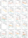 |
Fig. D.1 Final light curves. |
Appendix E Light-curve fitting examples
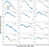 |
Fig. E.1 An example of light-curve fitting for SN 2018ilu in multiple filters using SALT3-NIR (green), BayeSN (orange), and SNooPy (purple). |
Appendix F Color terms
All Tables
Color-term coefficients for all filters using Emcee along with extinction coefficients.
SN types, coordinates, redshifts, host names, discovery and classfication groups and number of observations in the NIR.
Global photometry for our SN hosts using HostPhot along with host galaxy properties from Prospector.
Light curve parameters from SALT3 (t0,x0,x1,c), SNooPy (tmax,sBV,E(B–V)host) and BayeSN (PeakMJD,μ) along with peak apparent magnitudes in BJH. The errors are in the parentheses.
All Figures
|
Fig. 1 Example of a raw image reduction for an ANDICAM J-band image. Top row (left to right): single raw image of SN 2019so, master dark, and dark-reduced raw image using the two previous images and a master flat. Middle row: flat and dark-reduced image, detected cosmic rays, cosmic-ray-corrected image, and quadrant background level. Bottom row: image corrected for quadrant features, sky image, and sky-subtracted image. The sky image was evaluated from the remaining set of dithered images taken on the same night. The host galaxy was masked out for each single image when we constructed the sky image. |
| In the text | |
|
Fig. 2 Example of the background subtraction for a SOFI image. Left: combined J-band science image of SN 2018agk taken with SOFI. Middle: detected image background using photutils.BACKGROUND2D. Right: background- and cosmic-ray subtracted image. We were able to remove most of the quadrant structure from the image. |
| In the text | |
|
Fig. 3 Template subtraction using ImageMatch. Left: science image without template subtraction. Middle: fully subtracted science image. Right: template-subtracted image using ImageMatch with the SN in the middle of the subtracted area. ImageMatch does subtraction on the full image, but one can choose to have the subtracted area around the SN inserted back into the original science image. |
| In the text | |
|
Fig. 4 Example of measuring dDLR. The shape of the host was measured using sep and is plotted in orange. The dDLR is the ratio of the distance from the host center to the SN (purple) and the distance from the host center to the edge of the ellipse (dashed blue). |
| In the text | |
|
Fig. 5 Top panels: comparison of photometry using subtracted images (filled circles) vs. not using templates (empty circles) for SNe with different dDLR. Bottom: histogram of the apparent magnitude difference between subtracted and nonsubtracted images. The median value is reported in the legend for each filter. |
| In the text | |
|
Fig. 6 Aperture radii (orange for the local sequence and blue for a supernova) for one of our science images. The inset at the bottom right is a zoom-in of the SN and its aperture. |
| In the text | |
|
Fig. 7 Example of calculating an image zeropoint using bootstrapping with sigma clipping as outlier rejection, where the standard deviation from Chauvenet’s criteria was used. At the top of the panel, we show the image zeropoint and its error, the black line shows the fit using a linear function in the form of f(x)=x+b, the orange points represent the stars that remained after the sigma clipping, and the blue point(s) show rejected stars. The zeropoint is the intercept value from the fit. |
| In the text | |
|
Fig. 8 J-band zeropoints for different nights. The zeropoints were computed using Jinst−J2, where Jinst is the instrumental magnitude evaluated from aperture photometry, and J2 is the 2MASS catalog magnitude in the J band. Standards taken in the same night give different zeropoints, which makes the standards too uncertain. |
| In the text | |
|
Fig. 9 Sigma-clipped Bcat,std−Binst−ZPB,img,i vs. (B−V)cat,std for all B band images in the sample (black). We estimated binned means (red) and their uncertainties and removed very red/blue stars when the bins did not agree with the fit. The legend gives the slope using Scipy least squares (orange) and the MCMC fitting code Emcee (green), which shows that the values agree. |
| In the text | |
|
Fig. 10 Example of masking out stars using HostPhot. Left: initial image downloaded from Pan-STARRS. Middle: objects detected in HostPhot along with their apertures. Right: image without sources. |
| In the text | |
|
Fig. 11 Example of the SED fitting in Prospector. The black points show the flux (in maggies, where 1 maggie is equal to 3631 Jy) for our survey images. The fit SED profile is marked in brown, and the yellow boxes indicate the model value for a given survey. This is the initially detected aperture, not the final aperture measured by HostPhot. |
| In the text | |
|
Fig. 12 Comparison of Bmax estimates from BayeSN, SALT3-NIR, and SNooPy. |
| In the text | |
|
Fig. D.1 Final light curves. |
| In the text | |
|
Fig. E.1 An example of light-curve fitting for SN 2018ilu in multiple filters using SALT3-NIR (green), BayeSN (orange), and SNooPy (purple). |
| In the text | |
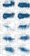 |
Fig. F.1 Same as Fig. 9, but for all ANDICAM and SOFI filters. |
| In the text | |
Current usage metrics show cumulative count of Article Views (full-text article views including HTML views, PDF and ePub downloads, according to the available data) and Abstracts Views on Vision4Press platform.
Data correspond to usage on the plateform after 2015. The current usage metrics is available 48-96 hours after online publication and is updated daily on week days.
Initial download of the metrics may take a while.