| Issue |
A&A
Volume 706, February 2026
|
|
|---|---|---|
| Article Number | A114 | |
| Number of page(s) | 16 | |
| Section | Galactic structure, stellar clusters and populations | |
| DOI | https://doi.org/10.1051/0004-6361/202556324 | |
| Published online | 09 February 2026 | |
Infrared photometry and calcium triplet spectroscopy of the most metal-poor in situ globular cluster VVV-CL001★
1
Departamento de Astronomia, Facultad de Ciencias, Universidad de La Serena.
Av. Raul Bitran 1305,
La Serena,
Chile
2
Instituto de Astronomía, Universidad Católica del Norte,
Av. Angamos 0610,
Antofagasta,
Chile
3
Observatorio Astronómico, Universidad Nacional de Córdoba,
Laprida 854,
X5000BGR,
Córdoba,
Argentina
4
Instituto de Astronomía Teórica y Experimental (CONICET-UNC),
Laprida 854,
X5000BGR,
Córdoba,
Argentina
5
Departmento de Astronomía, Universidad de Concepción,
Casilla 160-C,
Concepción,
Chile
6
Vicerrectoría de Investigación y Postgrado, Universidad de La Serena,
1700000,
Chile
7
Universidad Andres Bello, Facultad de Ciencias Exactas, Departamento de Física y Astronomía - Instituto de Astrofísica,
Autopista Concepción-Talcahuano 7100,
Talcahuano,
Chile
8
Gemini Observatory NSF’s NOIRLab,
670 N. A’ohoku Place, Hilo,
Hawaii,
96720,
USA
9
Rutgers the State University of New Jersey,
136 Frelinghuysen Ave.,
Piscataway,
NJ
08854,
USA
10
Preuniversitario Gauss,
Avda. Gabriela Mistral 2868,
La Serena,
Chile
11
Millennium Institute of Astrophysics,
Av. Vicuña Mackenna 4860,
782-0436
Macul, Santiago,
Chile
12
Instituto de Astrofísica, Pontificia Universidad Católica de Chile,
Av. Vicuña Mackenna 4860,
782-0436
Macul, Santiago,
Chile
13
Instituto de Astrofísica, Departamento de Física y Astronomía, Facultad de Ciencias Exactas, Universidad Andres Bello,
Fernandez Concha, 700,
Las Condes, Santiago,
Chile
★★ Corresponding author: This email address is being protected from spambots. You need JavaScript enabled to view it.
Received:
9
July
2025
Accepted:
11
November
2025
Abstract
Context. The characterization of globular clusters (GCs) in the Galactic bulge is a challenging task due to high extinction and severe stellar crowding. VVV-CL001 is a poorly studied GC located in the inner bulge, known for its extremely old age, extreme velocity, and low metallicity. Given its unique properties, a detailed study of this cluster can provide valuable insights into the early chemical and dynamical evolution of the Milky Way (MW).
Aims. The aim of this study was to derive the fundamental parameters of VVV-CL001 including metallicity, heliocentric radial velocity (RV), proper motions (PMs), structural properties, orbit, and age, in order to improve our understanding of its origin and role in the early evolution of the MW.
Methods. We combined spectroscopic, astrometric, and photometric data to characterize VVV-CL001. Metallicity and RV were determined from medium-resolution spectra obtained with FORS2 at the Very Large Telescope. PMs were derived using Gaia DR3 data. Near-infrared photometry from the FourStar instrument on Magellan was used to refine the cluster’s position, construct a radial density profile, and estimate its age, distance, and reddening.
Results. Our results confirm that VVV-CL001 is an old 12.1−1.2+1.0 Gyr), metal-poor ([Fe/H] = −2.25 ± 0.05 dex) globular cluster located at a heliocentric position of d⊙ = 7.1−1.1+1.3, with a reddening of E(J − Ks) = 1.40−0.02+0.01. Its mean PMs are μα* = −3.68 ± 0.09 mas yr−1 and µδ = −1.76 ± 0.10 mas yr−1, and it exhibits a RV of −334 ± 4 km s−1. The cluster follows a retrograde-prograde eccentric (e = 0.76−0.14+0.10) orbit, confined within the Galactic plane (|Z|max = 1.0−0.32+0.45 kpc) and inside the bar’s radius of influence (R < 5 kpc), with a pericenter of rperi = 0.6−0.2+0.3 kpc and an apocenter of rapo = 4.5−1.2+2.5 kpc.
Conclusions. These orbital properties, combined with its ancient age and low metallicity, strongly support an in situ origin for VVV-CL001 and likely membership of the disk GC system that was captured by the potential of the bar during its formation. Thus, VVV-CL001 emerges as a fossil remnant of the earliest phases of Galactic assembly and a valuable tracer of the population that contributed to the formation of the inner thick disk and bulge, which are likely part of the main progenitor of the MW. Our study highlights the relevance of detailed chemo-dynamical analyses in unveiling the origin of GCs in the inner Galaxy.
Key words: Galaxy: bulge / Galaxy: center / Galaxy: disk / Galaxy: formation / globular clusters: general
Based on observations gathered at the European Southern Observatory (programs ID 089.D-0392 and ID 091.D-0535A), at Las Campanas Observatory with the 6.5 m Magellan Telescopes (program ID CN2012A-034), and with the ESO-VISTA telescope (program ID 172.B-2002).
© The Authors 2026
 Open Access article, published by EDP Sciences, under the terms of the Creative Commons Attribution License (https://creativecommons.org/licenses/by/4.0), which permits unrestricted use, distribution, and reproduction in any medium, provided the original work is properly cited.
This article is published in open access under the Subscribe to Open model. This email address is being protected from spambots. You need JavaScript enabled to view it. to support open access publication.
1 Introduction
Globular clusters (GCs) are dense, gravitationally bound systems of tens of thousands to millions of stars concentrated in a small volume. Their member stars formed simultaneously from the same molecular cloud, giving them a common age and metallicity. GCs are among the oldest structures in the Universe, with ages ranging from 10 to more than 13 Gyr (e.g., Ying et al. 2023; Valcin et al. 2025). Virtually all of the older, more massive clusters display the multiple populations phenomenon. As such, they serve as important tracers of the formation and evolution of massive star clusters and indeed galaxies themselves (Gratton et al. 2019; Beasley 2020). The study of GCs provides key insights into the age, chemical enrichment history, kinematics, and dynamics of their host galaxies.
In the study of the formation and evolutionary history of the milky Way (MW), GCs have played a prominent role. Through them, we have learned much about the history of the halo, and have discovered that its population is largely accreted (Massari et al. 2019), corroborating what simulations had predicted (Tumlinson 2009). This was possible thanks to the accessibility of this component with its null or low extinction, which allowed the study of the GC population in the MW halo in great detail.
In contrast, simulations predicted that the bulge and disk populations of the MW are predominantly dominated by in situ population (Gargiulo et al. 2019; Bekki & Tsujimoto 2011), making the GC population in these regions of great interest for understanding the in situ formation and the early evolution of the proto-MW, dubbed the main progenitor. However, optical observations of these MW components are strongly inhibited by the presence of dust and gas, which generates high crowding, high and often variable extinction over even the small angular sizes of a GC at a distance of many kiloparsecs. Therefore, one must resort to observations at longer wavelengths that penetrate dust and gas, such as the near-infrared (NIR) (see Valenti et al. 2007; Lim et al. 2022; Cohen et al. 2018). In addition, crowding and field contamination also limit the study of these regions.
Over the past decades extensive photometric and spectroscopic surveys such as the Two Micron All Sky Survey (2MASS; Skrutskie et al. (2006)); the VISTA Variables in the Via Lactea Survey (VVV) and its extension, the VVVX Survey (Minniti et al. 2010; Saito et al. 2012; Smith et al. 2018); the Apache Point Observatory Galactic Evolution Experiment (APOGEE; Majewski et al. 2017); and the Gaia mission (Gaia Collaboration 2016, 2023) have provided an unprecedented amount of data for Galactic objects, allowing a much more comprehensive characterization of GCs. Additionally, observations from ground-based telescopes such as the Very Large Telescope (VLT) and GEM-INI, along with space-based observatories, for example the Hubble Space Telescope (HST) and the James Webb Space Telescope (JWST), have significantly contributed to the study of these systems by offering high-resolution imaging and spectroscopy in optical and infrared wavelengths to complement and augment the survey data. These studies have been instrumental in discovering and studying the structural and chemical properties of GCs. By combining astrometric, photometric, and spectroscopic information, researchers have refined the age–metallicity relation and calculated the orbital characteristics of most GCs, offering new insights into the assembly history of the Galaxy (Garro et al. 2021; Ceccarelli et al. 2024; Woody & Schlaufman 2021; Massari et al. 2019; Belokurov & Kravtsov 2023; Forbes & Bridges 2010; Cohen et al. 2021).
In this context, VVV-CL001 was the first GC discovered with the VVV survey (Minniti et al. 2011). Located in the Galactic bulge at coordinates l = 5.27◦, b = 0.78◦, it is projected very close to UKS1, a previously known GC, leading to speculation that both clusters might belong to the same system. Fernández-Trincado et al. (2021, hereafter FT21), using APOGEE high-resolution H-band spectra of two potential member stars and photometry from the VVV survey and 2MASS, determined that VVV-CL001 is located at a distance of  from the Sun, with an age of
  , a high heliocentric radial velocity (RV) of ∼−325 km/s, and an extremely low metallicity of [Fe/H] = −2.45 ± 0.24. They also derived an orbit, and found that it is halo-like and highly eccentric. Olivares Carvajal et al. (2022, hereafter OC22), analyzing much lower-resolution optical and NIR spectroscopic data from Multi Unit Spectroscopic Explorer (MUSE) for 55 stars in the field of the cluster and using photometry from VVV and VVVX, obtained similar values for the distance of 8.23 ± 0.46 kpc and a RV of −324.9 ± 0.8 km/s but a substantially higher, metallicity (albeit still very low) of [Fe/H] = −2.04 ± 0.02. They also concluded that it is basically confined to the bulge. These discrepancies in metallicity and orbit of the cluster highlight the need for more extensive spectroscopic studies to determine the true nature of VVV-CL001. Nevertheless, its extreme metallicity may point to an exotic early origin or unusual chemical enrichment conditions.
Belokurov & Kravtsov (2023) introduced a novel method to classify GCs as either in situ or accreted, based on their total energy (E) and the z-component of angular momentum (Lz), calibrated using [Al/Fe] abundance ratios. Applying this method to 165 GCs, they classified VVV-CL001 as an in situ object, agreeing with the orbital assessment of OC22 and in disagreement with the findings of FT21, who argued that the high orbital eccentricity of VVV-CL001 might instead favor a halo intruder and therefore accreted origin. This in situ classification is further supported by the recent CAPOS survey (Geisler et al. 2025), which analyzed bulge GCs and included VVV-CL001 in their in situ sample based on chemodynamical criteria. However, this contrasts sharply with the cosmological simulations of Boldrini et al. (2025), who identified VVV-CL001 as ex situ using a new energy threshold  . Such discrepancies underscore the challenges in disentangling the origins of GCs, particularly those in the bulge–halo transition region, where dynamical and chemical signatures often overlap.
All previous photometric analyses of VVV-CL001 were based on red-giant branch (RGB) stars, which are not ideal for precise age determinations since, the RGB locus is not very sensitive to age. This insensitivity arises because the RGB phase, while long-lived, converges stars of different initial masses onto a similar path in the color–magnitude diagram (CMD). Thus, the age of VVV-CL001 remains uncertain and needs to be determined using alternative methods. Deep photometric studies of the cluster can provide insight into evolutionary phases such as the subgiant branch (SGB) and the main sequence turnoff (MSTO), which are more suitable for age determination. Crucially, although the SGB phase is longer than the RGB phase for a given star, the position of stars on the SGB in the CMD is highly sensitive to their initial mass, and thus the cluster’s age. This sensitivity, combined with the shorter evolutionary timescales and larger separation between isochrones at the MSTO, makes these phases superior chronometers. Although current data for VVV-CL001, due to instrumental limitations, do not reach the MSTO, which is critical for deriving the most reliable age, incorporating SGB stars into the analysis represents a significant improvement over previous methods that rely solely on RGB stars.
In this work, we present a detailed analysis of the GC VVV-CL001 using spectroscopic data from the Focal Reducer and Low Dispersion Spectrograph 2 (FORS2) instrument on the Very Large Telescope (VLT), astrometric data from Gaia Data Release 3 (Gaia DR3), and photometric data from the VVV survey, 2MASS, and the FourStar instrument on the Magellan Baade Telescope. Our main objectives are to determine the cluster metallicity and age using both SGB and RGB stars and to study the cluster’s orbit within the Galaxy.
The paper is organized as follows. Section 2 describes the data and data reduction processes. Section 3 presents the methods used to determine the cluster’s RVs and metallicity. Section 4 discusses the analysis of IR photometric data, including the determination of the cluster’s center, density profile, proper motions (PMs), CMD, isochrone fitting; Section 5 explores the methodology used to determine the cluster’s Galactic orbit. Finally, Section 6 presents the discussion and our conclusions.
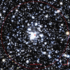 |
Fig. 1 False-color composite image using the infrared J (blue) and Ks (red) bands, centered on the GC VVV-CL001. The red dashed circle marks the core radius (rc = 0.′94), while the cross indicates the cluster’s central position. |
2 Observations and data reduction
2.1 Photometric data
Deep NIR photometric data were collected at Las Campanas Observatory during one night of observation on 2012 May 9, with the FourStar camera at the 6.5 m Baade telescope (program ID CN2012A-034, PI: S. Villanova). Five frames were collected into both the J and Ks bands, each one divided in four jittered sub-exposures, for a total exposure time of 38s (J band) and 6s (Ks) for each frame. The target cluster was not positioned at the center of the resulting 5.′7 × 5.′7 field to avoid the gaps between the four detectors. As a consequence, our data are limited to 3′ from the cluster center in the west direction (see Fig. 1).
The data were reduced using standard IRAF1 routines. The PSF photometry was performed with the VVV-SkZ_pipeline (Mauro et al. 2013), based on the DAOPHOT II and ALL-FRAME codes (Stetson 1994). The results were calibrated on the 2MASS astrometric and photometric system, as detailed in Moni Bidin et al. (2011) and Chené et al. (2012). The catalog was then cleaned of spurious detections, mainly found at redder colors around Ks ≈ 16, caused by defects of the detector and heavily saturated stars. Our FourStar photometry resulted more than two magnitudes deeper than VVV, but it lacked stars brighter than Ks = 12.6 due to saturation. We therefore obtained a shallower photometric catalog running the same pipeline on the VVV frames, and calibrated it on the 2MASS astrometric and photometric system. Then, we cross-matched the resulting catalogs, and added to our data the 2MASS and VVV sources undetected by FourStars, mainly bright objects up to Ks = 3. We thus eventually obtained our final photometric catalog, that includes 234 240 objects.
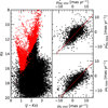 |
Fig. 2 Left panel: CMD of the VVV sources within 5′ of the cluster center with (red dots) and without (black dots) PMs from the Gaia catalog. Right panel: comparison of PMs in Galactic coordinates from Gaia and VVV. The red line indicates the fit of the data with a linear relation of unit slope. |
2.2 VVV proper motions
The large interstellar reddening along the line of sight (Minniti et al. (2011) estimate E(B − V) > 2.0) strongly limits the use of Gaia data, which are based on observations at visible wavelengths. The Gaia DR3 catalog (Gaia Collaboration 2023) reports PMs only for the bluest and brightest stars in the field, as shown in the left panel of Fig. 2. This covers only the brightest section of the cluster RGB, which is also scarcely populated, and hence only a few cluster stars are expected to be included in the catalog. We therefore measured PMs from 83 VVV epochs taken between 2010 and 2015. The VVV PMs were measured with the procedure described in detail in Contreras Ramos et al. (2017), which returns values relative to the mean motion of bulge RGB stars in Galactic coordinates ( , µb), where
  . We transformed these Galactic components to the equatorial ones (
 , µδ), where
  , by means of the formulae of Poleski (2013). The zero-point offset of the VVV relative PMs was determined from the axis intercept of the Gaia versus VVV relation for the ≈4200 stars in common, which was fit with a linear relation of unit slope, as shown in the right panels of Fig. 2. VVV frames saturated at Ks = 12.5, and the VVV PMs were eventually complemented with Gaia values for the brighter sources. The final PM catalog included ≈48 700 VVV sources down to Ks = 18.5 and within 5′ from the cluster center.
2.3 Spectroscopic data
Using the instrument FORS2 on the Very Large Telescope (Paranal, Chile), we obtained spectra of red giant stars belonging to the cluster VVV-CL001 and its surrounding field. The targets were selected according to their position in the cluster CMDs built from VVV photometry (Fig. 3). The observations were performed as part of the program 089.D-0392(PI: D Geisler) in service mode with the mask exchange unit (MXU), with the 1028z+29 grism and OG590+32 filter. The cluster was located in the master CCD and the secondary CCD was used for the observation of field stars. Slits located in the master and slave chips have a size of 1′′ wide and 4−8′′ long, and pixels were binned 2 × 2, yielding a plate scale of 0.′′25 pixel−1 and a dispersion of ∼0.85 Å pixel−1. The resulting spectra are centered in the Ca II triplet region (∼8600 Å) covering a spectral range from 7750 to 9500 Å. We obtained seven exposures of 660s each in order to reach an adequate final S/N. In this paper we only present the analysis of stars located in the master chip. The field star analysis will be included in an upcoming paper. We further note that these data were obtained during the same program as the other data reported in Geisler et al. (2023, hereafter G23).
The pipeline provided by ESO (version 2.8) was used to perform the bias, flatfield, and distortion correction and the wavelength calibration. The necessary calibration images were acquired by the ESO staff. We performed the extraction and the sky subtraction using the task apall of IRAF. IRAF was also used for the combination of the spectra (scombine task) and the normalization of the combined spectra (continuum task).
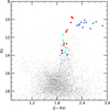 |
Fig. 3 Decontaminated VVV CMD of VVV-CL001. All sources detected within 1′ from the cluster center are shown as gray dots. Spectroscopic targets are marked as large colored points: blue, cyan, green and purple symbols are stars rejected as cluster members because they have a discrepant distance to the cluster center, mean RV, metallicity, and PMs, respectively. Red points represent spectroscopically confirmed cluster members. |
3 CaT spectroscopy
3.1 Heliocentric radial velocity and equivalent width measurements
We measured the RVs and the equivalent widths (EWs) of our targets following the method described in detail in G23. Briefly, we cross-correlated the observed spectra with template spectra, acquired with the same telescope and instrument, of stars belonging to Galactic open clusters and GCs (Cole et al. 2004) using the IRAF task fxcor. We adopt as the final RV the average of these cross-correlation results with a standard deviation of ∼6 km s−1. This standard deviation is added in quadrature to the error corresponding to the misalignment of the star in the slit (4.5 km s−1) to obtain the final adopted error for the RVs (7.5 km s−1). The procedure for correcting the effect introduced by the offset between the star and slit centers is explained in Parisi et al. (2009).
We used a combination of a Gaussian and a Lorentzian function (Cole et al. 2004) and the bandpasses from Vásquez et al. (2015) to measure the EWs of the CaT lines on the normalized spectra. The estimated errors in the EW measurements are in the range ∼0.–0.5 Å. As described in the next section, we followed the idea of G23 and calculated the cluster metallicity using three different calibrations: Vásquez et al. (2015), Vásquez et al. (2018), and Dias & Parisi (2020), hereafter V15, V18, and DP20, respectively. The sum of the EWs of the CaT lines (ΣEW) correlates with the metallicity of the clusters (Armandroff & Zinn 1988), and therefore the construction of this index is an important step. V15 and V18 are on the same scale as Saviane et al. (2012) and use only the two strongest CaT lines to calculate the ΣEW. In the case of DP20, all three CaT lines are used. The ΣEW from DP20 are based on the EW measurements from Parisi et al. (2009, 2015) so they are on the scale of Cole et al. (2004). In order to be completely consistent with these three calibrations, we calculate the ΣEW using the two strongest lines as well as all three lines. Saviane et al. (2012), V15, and V18 show that small differences exist between their EW measurements for the same spectrum even when the same pseudo-continuum and bandpass regions are adopted. Therefore, for the particular case of the calibration of V18 it is necessary to evaluate if such a difference is present between our EW measurements and those from V18. In G23 we used 119 spectra in nine Bulge Globular Clusters (BGCs) from V18 to perform this comparison. G23 found the following correlation between the sum of the EWs of the two strongest CaT lines between V18 and our work (OW):
 (1)
(1)
We then corrected our ΣEW from the two strongest lines according to Equation (1). As is shown in G23, this EW offset between the two studies implies a small error in the metallicity of only about 0.03 dex.
3.2 Metallicity determination and membership
The ΣEW depends not only on the metallicity, but also on the effective temperature and surface gravity (Armandroff & Da Costa 1991; Olszewski et al. 1991). These two latter dependences can be removed by the reduced EW (W′), which uses the dependence of these quantities along the upper giant branch and corrects for the difference of magnitude between the observed star and the horizontal branch in a particular filter. Much work has been carried out to calibrate ΣEW with metallicity using a variety of filters (see DP20 for a summary and compilation). In our case we used the Ks magnitudes from the VVV survey (Saito et al. 2012), so W′ can be expressed as follows:
 (2)
(2)
We used the corresponding  for the corresponding calibration:
  = 0.384 (V15),
  = 0.55 (V18) and
  = 0.37 (DP20).
To calculate Ks,HB we followed the procedure proposed by Mauro et al. (2014) which is explained in detail in Section 5 of G23.
The three calibrations used between [Fe/H] and W′ are:
![Mathematical equation: ${[{\rm{Fe}}/{\rm{H}}]_{{\rm{V}}15}} = - 3.150 + 0.432W' + 0.006{W^{\prime 2}},$](/articles/aa/full_html/2026/02/aa56324-25/aa56324-25-eq22.png) (3)
(3)
![Mathematical equation: ${[{\rm{Fe}}/{\rm{H}}]_{{\rm{V}}18}} = - 2.68 + 0.13W' + 0.055{W^{\prime 2}},$](/articles/aa/full_html/2026/02/aa56324-25/aa56324-25-eq23.png) (4)
(4)
![Mathematical equation: ${[{\rm{Fe}}/{\rm{H}}]_{{\rm{DP}}20}} = - 2.917 + 0.353W',$](/articles/aa/full_html/2026/02/aa56324-25/aa56324-25-eq24.png) (5)
(5)
We then calculated each target metallicity using the three calibrations, with a mean error of ∼0.20 dex. Following G23 we used the calibrations of V15, V18 and DP20 for comparison purpose, but our preferred calibration is V18 because it is based on the metallicity scale of Dias et al. (2016a,b). That scale includes MW GCs covering all the metallicity range of the bulge clusters. Therefore, in the subsequent analysis we used for our targets the metallicity values derived from the calibration of V18.
The applied discrimination method between cluster members and surrounding field stars is the same used by our group in previous work (Parisi et al. 2009, 2015; Dias et al. 2021, 2022; De Bortoli et al. 2022; Geisler et al. 2023). We refer to these papers for a detailed description but; briefly, the method discards as possible cluster members those targets that fall outside of certain cuts in distance from the mean cluster center, RV, and [Fe/H]. We adopted RV cuts of ±15 km s−1 and metallicity cuts of ±0.20 dex, which are typical errors for individual stars. The cluster core radius (rc = 0.′94) was adopted as the distance cut, in order to maximize the probability that the selected stars are members of the cluster (see Sect. 4.1 and Fig. 4).
The behavior of RV and metallicity, respectively, with distance from the cluster center are shown in Fig. 4. Fig. 5 shows the PM plane for CL001 where targets (large colored points) are plotted jointly with stars from the Gaia DR3 catalog centered on the cluster coordinates. In these plots we represent targets with the following color-coding (the same used in our previous work; e.g., G23): blue symbols represent field stars located at a distance from the cluster center larger than the adopted radius, cyan and green are for stars with RV or metallicity, respectively, outside the adopted cuts. We finally check that the stars that have passed these three cuts also have similar PMs (Fig. 5). Targets rejected because of their discrepant PMs are marked in purple. Finally, the seven stars that passed all the membership criteria, and therefore are considered cluster members, are plotted in red.
For cluster members we include in Table 1 the star identification, the equatorial coordinates, RV, Ks − Ks,HB, the sum of the measured EWs of the CaT line (ΣEW2L for two lines and ΣEW3L for three lines), the V18 metallicity, and the PMs. Using the information of this table and Equations (3) and (5) individual metallicities using V15 and DP20 calibrations can be straightforwardly calculated.
Using cluster member stars, we calculate mean values of [Fe/H]V15 = −2.31 ± 0.08 dex, [Fe/H]V18 = −2.25 ± 0.05 dex, [Fe/H]DP20 = −2.13 ± 0.09 dex, RV = −339.7± 3.5 km−1,  = −3.33 ± 0.10 and µδ = −1.61 ± 0.11 for cluster mean RVs, metallicity and PM, respectively. The quoted errors correspond to the standard error of the mean. As we found in G23 for a sample of 12 BGCs, the mean metallicities corresponding to the V15 and DP20 calibrations maintain good agreement with the values given by the V18 calibration.
Our sample has some stars in common with previous spectroscopic works. In particular, five cluster member stars in our sample were previously observed with MUSE (OC22) and two with APOGEE (FT21). Table 2 includes a comparison between the metallicity values obtained by the different works. As can be seen, the metallicity values derived in this work show a very good agreement with those derived by FT21 for the 2 stars in common. However, the values from OC22 present a mean offset of 0.27 dex with respect to our determinations.
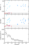 |
Fig. 4 Upper panel: RV of the spectroscopic targets as a function of distance from the cluster center. The horizontal lines represent our velocity cuts (±15 km s−1). Middle panel: metallicity of the spectroscopic targets as a function of distance from the cluster center. The horizontal lines represent our metallicity cuts (±0.20 dex). For both panels the color-coding is the same as in Fig. 3. Lower panel: radial density profile of the photometric sources with respect to the cluster center. The dotted curve indicates the best fit of a King (1962) radial profile. |
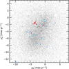 |
Fig. 5 PM plane for cluster VVV-CL001.The gray points stand for stars from the Gaia DR3 catalogue and the large colored points represent our spectroscopic targets. The color-coding is the same as in Fig. 3. |
Measured values for member stars.
Comparison with previous spectroscopic metallicity determinations.
4 Infrared photometry
4.1 Cluster center and density profile
To determine the center of the cluster, we first calculated the average position of all the sources detected within 0.′5 from the center given by Minniti et al. (2011). The result was used as the new center and the procedure iterated until convergence. The position of the center changed by less than 0.′′2 at each iteration, and eventually converged to the coordinates (RA, Dec)=(17h54m42.s22, −24◦00′52.′′3), only 1.′′8 away from the original center of Minniti et al. (2011).
The cluster density profile was obtained by measuring the stellar density in concentric annuli of width ∆r = 0.′14, centered at the coordinates derived above. We also considered different binning schemes, including wider, narrower, and/or overlapping annuli, but found no substantial difference in the results. The profile was not extended beyond 2.′5 from the center, where the mosaic nature of our photometric catalog caused a sudden discontinuity of the source density in the northwestern direction. The results are shown in the lower panel of Fig. 4, where the vertical bars indicate the Poissonian errors of stellar counts. In the figure we also show a tentative fit of the data with a King (1962) profile, which returns rc = 0.′94 and rt = 3.′48 for the core and tidal radius, respectively. These results suggest that VVV-CL001 is a small (rt = 7.6 pc at a distance of 7.5 kpc) and sparse (concentration parameter c = 0.57) object, very similar to the smallest Galactic GCs such as Whiting 1 (c=0.55, Carraro et al. 2007), FSR1735 (c=0.56, Carballo-Bello et al. 2016), and Palomar 10 (c=0.58, Kaisler et al. 1997). However, we consider this result only indicative and not fully reliable because a King profile should be inappropriate to describe a small cluster embedded in the gravitationally complex inner Galactic regions. Deviations from the King profile should be expected, in particular at intermediate radii between the innermost and the external regions, which tend to push the fit profile to higher rt and rc and lower c, as previously observed in similar situations (e.g., Moni Bidin et al. 2011; Carballo-Bello et al. 2016).
4.2 Proper motions
Figure 5 shows the PMs of all the Gaia-VVV sources within 5′ from the cluster center. Two main populations can be identified, with approximately elliptical distributions around the points  mas yr−1 and ≈ (−0.5, −2.0) mas yr−1. An inspection of the CMD reveals that the first population is clearly more distant and redder, and it lacks a noticeable group of young blue stars. These characteristics identify it as the bulge main stellar population. The second group, on the other hand, is rich in blue main sequence stars, corresponding to the foreground disk.
In the same figure, we also show the PMs of the spectroscopic targets, coded with the same colors as in Fig. 4. The stars identified as cluster members (red dots) clearly reveal the cluster. However, the small cluster is embedded in a crowded area, and its PM is not too different from the field. As a consequence, no overdensity of stars can be identified at this position in the general PM catalog, even if restricted to stars within 1′ from the center. We therefore cleaned the diagram from the field contamination, with a statistical algorithm similar to that employed later in the CMD (Sect. 4.3), but applied to the PM plane. In brief, we created a cluster catalog with all the sources within 1′ from the cluster center, and a comparison field catalog with the stars in an annulus of equal area and inner radius of 2′. This selection was made based on the density profile shown in Fig. 4. Then, the closest source in the field catalog was identified for each object in the cluster area, and if the distance was lower than 1 mas yr−1, both stars were removed from their respective catalogs. The objects of the cluster area that survived this procedure formed our final cluster catalog cleaned from field contamination, and they are indicated in Fig. 5 as color dots. Apart from some scarce and scattered residual contamination, the position of the cluster thus can be properly identified. We derived the cluster PM as the weighted average of the clumped stars in the de-contaminated list, to which we added the spectroscopically confirmed cluster members, finding  = (−3.68 ± 0.09, −1.72 ± 0.12) mas yr−1. Our results agree within approximately 1σ with those of Vasiliev & Baumgardt (2021) and FT21, while we have irreconcilable differences in the component µδ with OC22, as summarized in Table 3.
Cluster PMs from the literature.
4.3 Color–Magnitude diagram
We cleaned the CMD from field contamination following the procedure of Moni Bidin et al. (2011) and Moni Bidin et al. (2021), based on the method described by Gallart et al. (2003). For each star in the field region, the algorithm identifies the nearest star in the cluster region in terms of a distance metric d in the CMD, defined as:
 (6)
where k is an arbitrary coefficient that weights the color differences relative to magnitude differences. If d is smaller than a given threshold (dmax), the star is removed from the cluster catalog. For this study, we adopted k=2 and dmax = 0.3 (see Moni Bidin et al. 2021, for a discussion on these parameters). The cluster region is defined as a circular area with a radius of rc = 0.′94 around the estimated center (Section 4.1), while the field region is selected as an annular region with an inner radius of rin = 1.′2, chosen so that its area matches that of the cluster region.
(6)
where k is an arbitrary coefficient that weights the color differences relative to magnitude differences. If d is smaller than a given threshold (dmax), the star is removed from the cluster catalog. For this study, we adopted k=2 and dmax = 0.3 (see Moni Bidin et al. 2021, for a discussion on these parameters). The cluster region is defined as a circular area with a radius of rc = 0.′94 around the estimated center (Section 4.1), while the field region is selected as an annular region with an inner radius of rin = 1.′2, chosen so that its area matches that of the cluster region.
Any statistical decontamination procedure is based on the underlying hypothesis that the photometric properties of the contaminating field stars are identical to those in the control area. Large reddening variations in the field could violate this hypothesis, and cause the removal of the wrong stars in the cluster area, thus spoiling the results. We performed a series of decontamination tests to verify this possibility and to ensure the robustness of our results. We first selected eight circular regions of radius 0.′4, located at a distance of 1.′5 from the estimated cluster center, and we ran the decontamination procedure on each of them using as field area the circular region on the opposite side with respect to the cluster. This test revealed small but non-negligible residuals in the decontaminated CMD, due to the presence of a reddening gradient in the direction of the Galactic center, which is only 5.◦5 away. However, the residuals disappeared when we decontaminated an annular region using another annular area with larger inner radius as the control field. This showed that the annular symmetry is enough to compensate for the smooth variations of reddening in the field, and the cluster decontamination is therefore reliable.
Figure 6 shows the result of the statistical decontamination process with the orange points. The RGB is clearly visible at magnitudes brighter than ∼16. At fainter magnitudes, the SGB is less evident due to larger photometric errors and some residual contaminating stars.
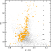 |
Fig. 6 CMD of the photometry obtained in the VVV CL001 field within a radius of 0.′94 from the center of the cluster (gray points). The orange points are the stars resulting from the statistical decontamination process. The black symbols give the average photometric errors per magnitude bin. |
4.4 Reddening and age determination
The age of VVV-CL001 was determined through isochrone fitting to NIR CMDs constructed using J, H, and Ks photometry (Section 4.3), in combination with theoretical isochrones from the PARSEC database (Bressan et al. 2012). A full description of the method is provided in Appendix A; we summarize the key aspects here.
Isochrone fitting depends on four parameters: age, metallicity, apparent distance modulus (µKs), and reddening (E(J − Ks)). In our analysis, the metallicity was fixed at [Fe/H] = −2.25 ± 0.01 dex, as derived in Section 3.2. To reduce degeneracies, E(J − Ks) and  were parameterized relative to a fiducial point (FP) placed on the RGB, where the sequence is well-defined and age-insensitive. The adopted FP coordinates are (J − Ks, Ks) = (1.92, 13.72) mag (Fig. 7, black cross).
We employed an iterative convergent approach to determine the best-fitting isochrone. Initial grids of theoretical isochrones spanning 7–13 Gyr were shifted across a range of E(J − Ks) and µKs values consistent with the FP. The optimal combination of E(J − Ks) and  was identified by minimizing the metric M (Eq. (A.4)), which quantifies the distance between the shifted isochrone and the observed CMD (inner panel of Fig. 7). With these values fixed, the best-fitting age was determined by minimizing the absolute mean residual
  (Eq. (A.6)), computed along the extinction vector and restricted to the SGB (J − Ks < 1.8 mag) to maximize age sensitivity. The process was repeated iteratively until the age varied by less than 0.1 Gyr between iterations, and consistent results were obtained whether starting from 7 or 13 Gyr, hence the term convergent approach.
The final best-fitting isochrone is overplotted on the CMD in Fig. 7. We derive an age of  , with reddening
  mag and distance modulus
  mag. The left panel of Fig. 8 shows the behavior of
  as a function of age, with a clear minimum at 12.1 Gyr. The right panel illustrates the variation in the residual R with color for a subset of isochrones; the shaded region (J − Ks > 1.8 mag) was excluded from the fit due to the weaker age sensitivity of the RGB.
Uncertainties in the age were estimated by repeating the fitting process while varying the E(J − Ks),  , and metallicity within their respective errors. The individual contributions to the age uncertainty were determined as follows: metallicity variations yielded an uncertainty of
  , while the combined variation in E(J − Ks) and
  , which are correlated parameters resulted in an uncertainty of
  . The final age uncertainty was computed as the quadratic sum of these deviations, giving
  Gyr.
Gyr.
Although a reddening gradient toward the Galactic center was identified in Section 4.3, tests confirmed that its effect on our results is negligible and already accounted for in the error estimates. We note that our photometry does not reach the main sequence turnoff, but does include the SGB, which provides a more reliable age diagnostic than previous results. Our final age is consistent within 1σ with the value of  reported by FT21.
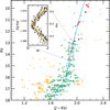 |
Fig. 7 CMD of VVV-CL001. The green points represent stars retained after the re-decontamination process, while the orange points indicate the rejected stars. The red points correspond to CaT-confirmed members of VVV-CL001. The black cross marks the adopted fiducial point, and the blue curve shows the best-fitting theoretical isochrone. Inset: value of the metric M (Eq. (A.4)) for each tested combination of E(J − Ks) and |


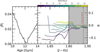 |
Fig. 8 Left panel: mean absolute residual |

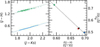 |
Fig. 9 Left panel: Color–Color diagram. Green points: only RGB stars from the photometric data resulting from statistical decontamination. Blue points: best-fit isochrone model from Section 4.4. The green and blue dotted curves show the linear fit of the green and blue points, respectively. Right panel: plane of |


4.5 Distance
The cluster distance can be derived from the apparent distance modulus  and the reddening E(J − Ks) only if the extinction law along the line of sight is well constrained (Cardelli et al. 1989). However, fluctuations in the density and composition of interstellar dust in the direction of the Galactic bulge (Nataf et al. 2010) introduce significant variations in the extinction law, and they complicate photometric measurements and precise distance estimates (Minniti et al. 2010; Gonzalez et al. 2012). Although NIR extinction is lower than in optical wavelengths, it remains a crucial factor that must be carefully modeled to minimize its effects on photometry and distance determination (Indebetouw et al. 2005).
The left panel of Fig. 9 shows our determination of the color excess E(J − H) by comparing the observed cluster RGB with the theoretical isochrone in the (J − H) versus (J − Ks) diagram. The theoretical isochrone corresponds to the best-fitting model from Section 4.4 and includes evolutionary stage labels (1: main sequence (MS), 2: SGB, 3: RGB, 4: asymptotic giant branch). We corrected the isochrone for the adopted values of E(J − Ks) and distance modulus  determined in Section 4.4, which allowed us to estimate the RGB sequence in the observational data. The vertical separation between the reddening-corrected observational data and this isochrone returned E(J − H) = 0.95± 0.01. This analysis confirms the nearly linear trend of both RGB and SGB sequences in the color-color diagram, though we note that potential spurious detections in the SGB region could slightly affect its linear fit.
Since VVV-CL001 is located in the Galactic bulge, the standard extinction law of Cardelli et al. (1989) is not suitable. Instead, the extinction law from Nishiyama et al. (2009) is more appropriate. However, this study does not cover the specific region in which VVV-CL001 is located. To determine the most applicable extinction law for the cluster, we interpolated the values of  given in these two studies, as a function of E(J − H)/E(J − Ks), as shown in Fig. 9. This interpolation yields
  for the value E(J − H)/E(J − Ks) = 0.68 ± 0.01 previously obtained for VVV-CL001. Our result is consistent with the average of the four quadrants studied by Nishiyama et al. (2009), but it deviates from the quadrant that is closest to the position of the cluster.
Finally, the cluster’s distance was determined using the distance modulus relation:
![Mathematical equation: ${{\rm{d}}_ \odot } = {10^{\left[ {{\mu _{Ks}} + 5 - E\left( {J - {K_s}} \right){{{A_{Ks}}} \over {E\left( {J - {K_s}} \right)}}} \right]/5}}$](/articles/aa/full_html/2026/02/aa56324-25/aa56324-25-eq54.png) (7)
with
(7)
with  and E(J − Ks) obtained in Section 4.4,
  determined in this section,
  the extinction in the Ks band, and d⊙ the distance in parsecs. The cluster distance was computed as
  . The uncertainty was estimated following a procedure similar to that in Section 4.4. The individual contributions to the distance uncertainty were determined as follows: metallicity variations yielded an uncertainty of ±0.2 kpc, while the combined variation in E(J − Ks) and
  , which are correlated parameters resulted in an uncertainty of
  . The final distance uncertainty was computed as the quadratic sum of these deviations. Our distance estimate is in agreement within the error bars with that reported by FT21, who determined a distance of
  . Similarly, we achieve agreement within the error bars with what was reported by OC22, who determined a distance of 8.23 ± 0.46 kpc. However, it should be noted that the latter mentions that their value should be considered an upper limit for the distance of VVV-CL001. The discrepancies between the mean values we found and those in the literature may be primarily due to the methodology used in these studies, as well as the extinction law applied in each estimation. The latter, in particular, can cause significant differences with small variations in the extinction value used.
5 Orbital properties
We derived the main orbital properties of VVV-CL001 using the observational estimates in Table 4 as initial conditions, and for the orbital calculations we used the software DELOREAN (Blaña et al. 2020). This code has an updated MW potential (Blaña et al. in prep.) that includes the MW bulge–bar stellar mass component of Sormani et al. (2022, hereafter S22), which was derived from made-to-measure models fitted to the observations (Wegg & Gerhard 2013; Portail et al. 2017). This bar model consists of an inner disky component, a thick box/peanut bulge structure extending ∼2 kpc in radius and ∼1 kpc in height, a flat or thin bar component that extends to 5 kpc in radius and 45 pc height, and another stellar disk (Bland-Hawthorn & Gerhard 2016, hereafter BG16). We adopted the bar pattern speed angular frequency of  km s−1 kpc−1 rad (equivalent to a rotation period of Tbar = 157 Myr) (Portail et al. 2017) and a bar angle of −27o (Wegg & Gerhard 2013), which encompasses other estimates in the literature within the errors. The potential model also includes components for the dark matter halo, gaseous disk, and nuclear components. In Appendix B we provide additional information, as well as the circular velocity profiles of the potential model (see Fig. B.1). For the solar parameters, we adopted the values of BG16 for the Sun’s galactocentric distance of R0 = 8.2 ± 0.1 kpc, a vertical height of z0 =25 ± 5 pc, and the solar constants of motion of (u⊙, v⊙, w⊙) = (1±1, 248±3, 7.3±0.5) km/s. With this we estimate that the current galactocentric distance of VVV-CL001 is
  and its distance from the Galactic mid-plane is
  , with errors derived from a Monte Carlo propagation of the errors of the cluster coordinates and the solar constants.
Considering this setup for the potential and the cluster coordinates, we computed the orbital properties of VVV-CL001. To explore the effects of the uncertainties, we adopted a Monte Carlo method by randomly sampling 104 values from normal distributions with standard deviations with sizes taken from the estimated errors in the coordinates shown in Table 4. We also sampled values for the bar pattern speed to account for this uncertainty. We took the orbital integration time of 6 Gyr (5 Gyr into the past and 1 Gyr into the future). While arbitrary, this time is long enough to consider multiple orbital timescales for the cluster to explore phase-space, where we find typical orbital periods of Tϕ ∼ 100 Myr. Longer orbital integrations would be comparable to changes in the MW potential evolution and/or possible orbital interactions, which would propagate these time-dependent uncertainties into the orbital parameters. Furthermore, we tested longer or shorter integration time intervals, and found similar results. From the resulting orbital distributions, we calculated the medians and 1σ confidence values of the orbital properties such as the pericenter (rperi), the apocenter (rapo), the maximum vertical height (|Z|max), eccentricity (e = (rapo − rperi)(rapo + rperi)−1), and additional relevant orbital properties. These properties were then compared with the current structural properties of the MW bulge, bar and disk. We note that in this reference system, where the Sun is located at X =−8.2 kpc, the MW disk and bar have a clockwise rotation and therefore, they have negative Z-axis specific angular momentum (lz < 0 kpc km/s).
We present the orbital computations of VVV-CL001 in Fig. 10, showing the orbit with the most likely position and a subsample of randomly selected orbits. We used the total sample of 104 orbits to calculate the distribution of the orbital parameters, presenting their medians and 1σ percentile intervals in Table 5. An inspection of Fig. 10 of the sample of possible orbits and the density probability maps reveals that the cluster lives orbiting the volume occupied by the bar and inner disk. It enters the disk region when it approaches its orbital apocenter (rapo = 4.5 kpc), and it enters the bar and central bulge when it reaches its pericenter (rperi =0.6 kpc). Moreover, we find that the orbits remain vertically close to the disk and box/peanut bulge of the MW, extending only out to |Z|max = 1 kpc. It orbits around the MW every Tϕ =107 Myr, while it enters the central region of the box/peanut bulge every TR =55 Myr, approaching the epicycle approximation (Tϕ ∼ 2TR), and a vertical period around the mid-plane every TZ =71 Myr.
We also measured the specific angular momentum of the orbit of the cluster around the MW’s rotation axis (lz) finding that it is not conserved, which is expected for a triaxial rotating potential such as the MW bar. We measured whether the cluster orbit is prograde (lz < 0 kpc km s−1) or retrograde (lz > 0 km s−1 kpc) with respect to the MW (here lzMW < 0 km s−1 kpc). We find that with the current observed positions and velocity distributions, lz has a median and deviations of  ; within the observational errors, we find prograde (28%) and retrograde (72%) orbital directions. However, given that the cluster constantly crosses between the outer and inner regions of the bar near the mid-plane, the rotating potential can perturb the orbits generating a chaotic behavior that can frequently flip the direction of rotation of the orbit, making prograde-retrograde orbits. Therefore, the median of lz covers prograde and retrograde phases with
  , where the minima of lz have a range of
  , while the maxima have lzmax = 128 ± 150 km s−1 kpc. This chaotic orbital behavior has already been identified in other star clusters in the MW (e.g.; Pichardo et al. 2004; Pérez-Villegas et al. 2018, 2019; Tkachenko et al. 2023).
We also performed tests computing the orbital properties in different potentials, using an adaptation from Plotnikova et al. (2023), and find similar values for the apocenter (rapo = 6.4 ± 1.3 kpc), the pericenter (rperi = 0.37 ± 0.16 kpc), and a vertical height of |Z|max = 0.65 ± 0.09 kpc. The differences arise due to differences of the bar mass model. To test the effects of the bar on the orbital properties, we implemented the axisymmetric MW potential MWPotential2014 from Bovy (2015) into DELOREAN. We find similar overall orbital properties, such as the orbital periods, with some differences due to conserved quantities (e.g., lz) allowed by the barless potential, producing orbits more confined to the plane of the Galaxy with  , reaching pericenter and apocenter means of
  and
and  , respectively.
Consequently, considering the orbital distribution of the cluster that concentrates its orbit around the box/peanut bulge and bar within r ∼ 5 kpc, while reaching the central region around r ∼ 0.6 kpc, its relative confinement on the vertical axis (|Z|max ∼ 1 kpc), its old age (12.1 Gyr), and its metal-poor content, we propose a scenario where this cluster was formed in the very early disk before the formation of the bar. Then it was captured during the formation of the bar, between 8 and 10 Gyr ago (Sanders et al. 2024, see also Schoedel et al. (2023)), it was then pulled into higher orbits in Z through heating mechanisms, such as bar buckling and satellite interactions. We also compared the orbital properties of VVV-CL01 with the GC orbital classification of Pérez-Villegas et al. (2019, see their Fig. 6), and find that this cluster would agree with both thick disk and the bulge–bar GC populations.
We also compared specific studies of VVV-CL001 in the literature. FT21 explored a vast parameter space, and presents different orbital solutions that depend on the adopted observational coordinates of the cluster, finding some prograde-retrograde solutions, and concluding that the star cluster could be associated with halo-like orbits and accretion events. In general, we find good agreement with their orbital calculations, particularly with their model with a cluster distance of d⊙ = 7.87−8.10 kpc, which results in a Jacobi (energy) integral and orbital energy values that can also be associated with the box/peanut bulge (see their Fig. 4). On the other hand, the model of Vasiliev & Baumgardt (2021) produces more compact orbits of rapo ∼ 2 kpc, always retrograde and regular orbits, which is due to the compact (barless) spherical bulge potential used in their models (McMillan 2017; Bovy 2015, MWPotential 2014), and due to differences in the observed coordinate values. Using the same models for the potential, OC22 determines that for this cluster rapo ∼ 3.2 kpc; given its position and very low velocity, this suggests that it is associated with the bulge or inner halo rather than with the thick disk. Moreover, in addition to the MW potential, our error propagation study shows that the cluster’s distance is the most critical variable that determines its orbital history as this cluster is so close to the bulge center ( ), where the potential is deepest. Deviations of ±1 kpc significantly change its orbital energy, as well as the conversion from PMs to physical velocities.
Derived cluster parameters.
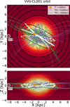 |
Fig. 10 Orbital calculations for VVV-CL001. We show the most likely current position (large orange circle) and the corresponding orbit (white curve) showing its past −150 Myr orbit (solid) and future 150 Myr orbit (dashed) seen in the X −Y plane view (top panel) and the X −Z view (bottom panel). To avoid crowding we show a subsample of 20 randomly selected orbits from the total of 104 orbits, giving their current positions (smaller circles), their past orbits (green) and future orbits (purple). The density probability (color map) shows the regions that the orbits inhabit. The stellar surface mass density contours of the MW bar and inner disk model of S22 reveal that this cluster lives between the inner disk and the bulge–bar region. We also plot the Sun’s position. We note that in this frame the MW and the bar rotate clockwise, with the bar havings a rotation period of Tbar =157 Myr. |
VVV-CL001 orbital parameters.
6 Discussion and conclusions
Our study provides a detailed characterization of the unique GC VVV-CL001, establishing it as an ancient in situ and metal-poor object located in the Galactic bulge region. The results show both agreements and discrepancies with previous studies. The derived coordinates differ by 1.′′8 compared to Minniti et al. (2011). The structural parameters obtained, with a core radius of rc = 0.′94 and a tidal radius of rt = 3.′48, suggest that it is a relatively compact cluster.
Regarding kinematics, the PMs obtained are consistent within 1σ with those of Vasiliev & Baumgardt (2021) and FT21, but show an irreconcilable difference in the component of µδ with those of OC22 (see Table 3). The RVs obtained in this work, RV = −334 ± 4 km s−1, is similar to the values reported by FT21 and OC22, who find approximately −325 km s−1 and −324.9 ± 0.8 km s−1, respectively. Methodological differences between these works could explain the small discrepancies. The metallicity value of [Fe/H] = −2.25 ± 0.05 obtained in this study is consistent with that of FT21 but not with that of OC22, who report −2.45 ± 0.24 and −2.04 ± 0.02, respectively.
However, we find significant differences in the reddening affecting the cluster. Our value of E(J − KS ) = 1.40 differs from the value of ∼1.34 adopted by OC22 in the determination of their distance. The distance derived in this work, d⊙ = 7.1 kpc, agrees within 1σ with that of FT21 but not with that of OC22. However, OC22 note that their reported distance should be considered an upper limit for VVV-CL001, and under this context, our results are consistent. Finally, our age estimate of  Gyr is consistent with that of FT21, while OC22 did not report an age estimate.
Based on our results, we can explore the possible origin of VVV-CL001. Its low metallicity and age suggest that it formed at a time when the interstellar medium had not yet been significantly enriched by supernova Ia explosions (Marin-Franch et al. 2009; Lahén et al. 2019; Chiti et al. 2021). However, to confirm this hypothesis, a more detailed spectroscopic analysis of the cluster’s stellar population is required. In this sense, conducting high-resolution NIR spectroscopic studies, similar to that of FT21 but for a larger sample of stars, would be crucial in order to continue investigating the early formation and evolution processes of this GC and, consequently, to help recover the formation history of the MW.
We also calculated the orbital properties of VVV-CL001 with updated Galactic potentials (see Section 5). We find that the cluster has a prograde-retrograde orbit type due to the barred potential (see Tkachenko et al. 2023). The orbits are eccentric (e=0.76), traveling between the box/peanut bulge central region (rperi = 0.6 pc) and the flat bar and disk region (rapo = 4.5 kpc). Moreover, the orbit lies confined within |Z|max ∼ 1 kpc from the disk mid-plane, suggesting a connection with this structure.
These orbital properties strongly suggest an in-situ origin in the early proto-Galactic disk, before the formation of the bar. It is likely that the cluster was captured by the bar’s gravitational potential in its early stages, being vertically lifted from the galactic mid-plane through dynamical mechanisms, such as the bar buckling that formed the boxy/peanut bulge, or satellite interactions. Thus, VVV-CL001 would be a fossil remnant from the earliest phases of Galactic assembly and a valuable candidate for being part of the population that gave rise to the inner disk and bulge. It is currently the most metal-poor in situ GC known with a well-determined metallicity (Geisler et al. 2025), and further study will help reveal conditions in the early history of the main progenitor of the MW.
The main uncertainties in this study arise from the lack of our knowledge of the extinction law for this region of the Galaxy, affecting the precise distance determination. Additionally, the photometry used was limited by spurious detections in the catalog and the inability to accurately characterize the cluster’s turnoff, which limits the precise age estimation.
To improve the characterization of VVV-CL001, deeper photometry is essential, and would allow a more accurate determination of the cluster’s age and other evolutionary parameters. Moreover, the development of a more detailed extinction law for the Galactic disk and bulge region would be crucial to reduce uncertainties in the distance determination, as this is the parameter that most strongly affects age estimation according to Ying et al. (2023), given sufficiently deep photometry well below the MSTO. We note that we are currently obtaining very deep J and Ks images for VVVCL1 from the GEMINI-S GeMS + GSAOI instrument, which should reach several magnitudes below the MSTO and provide a much more precise and accurate age.
This work represents one of the most comprehensive studies to date on VVV-CL001, combining astrometric, photometric, and spectroscopic information to characterize its nature. The methodology used to determine its age, distance, and metallicity provides a solid framework for future studies of GCs in highly extincted regions of the MW. Finally, the possibility that VVV-CL001 is a relic from the early stages of Galactic formation makes it an ideal candidate for more detailed studies, combining PM information with high-resolution spectroscopic data. It may well be the oldest remnant of the MW main progenitor, and a reliable age and more detailed chemistry will help constrain the formation and early chemical evolution of the main progenitor and place a lower limit to the age of the MW and indeed of the Universe.
Acknowledgements
This work has made use of data from the European Space Agency (ESA) mission Gaia (https://www.cosmos.esa.int/gaia), processed by the Gaia Data Processing and Analysis Consortium (DPAC, https://www.cosmos.esa.int/web/gaia/dpac/consortium). Funding for the DPAC has been provided by national institutions, in particular the institutions participating in the Gaia Multilateral Agreement. D.G. gratefully acknowledges the support provided by Fondecyt regular no. 1220264. D.G. also acknowledges financial support from the Dirección de Investigación y Desarrollo de la Universidad de La Serena through the Programa de Incentivo a la Investigación de Académicos (PIA-DIDULS). C.M. thanks the support provided by ANID-GEMINI Postdoctorado No.32230017. S.V. gratefully acknowledges the support provided by Fondecyt Regular n. 1220264 and by the ANID BASAL project FB210003. B.D. acknowledges support from ANID Basal project FB210003. M.B. thanks M.A. Perez Villegas and M. De Leo for helpful discussions. Finally, We thank the referee for their rigorous corrections, which significantly improved the clarity and precision of the manuscript. We also thank the language editor for polishing the manuscript.
References
- Armandroff, T. E., & Da Costa, G. S. 1991, AJ, 101, 1329 [Google Scholar]
- Armandroff, T. E., & Zinn, R. 1988, AJ, 96, 92 [Google Scholar]
- Beasley, M. A. 2020, Globular Cluster Systems and Galaxy Formation (Berlin: Springer International Publishing), 245 [Google Scholar]
- Bekki, K., & Tsujimoto, T. 2011, MNRAS, 416, L60 [NASA ADS] [CrossRef] [Google Scholar]
- Belokurov, V., & Kravtsov, A. 2023, MNRAS, 528, 3198 [Google Scholar]
- Blaña, M., Burkert, A., Fellhauer, M., Schartmann, M., & Alig, C. 2020, MNRAS, 497, 3601 [CrossRef] [Google Scholar]
- Bland-Hawthorn, J., & Gerhard, O. 2016, ARA&A, 54, 529 [Google Scholar]
- Boldrini, P., Di Matteo, P., Laporte, C., et al. 2025, A&A, 704, A81 [NASA ADS] [CrossRef] [EDP Sciences] [Google Scholar]
- Bovy, J. 2015, ApJS, 216, 29 [NASA ADS] [CrossRef] [Google Scholar]
- Bressan, A., Marigo, P., Girardi, L., et al. 2012, MNRAS, 427, 127 [NASA ADS] [CrossRef] [Google Scholar]
- Carballo-Bello, J. A., Ramírez Alegría, S., Borissova, J., et al. 2016, MNRAS, 462, 501 [NASA ADS] [CrossRef] [Google Scholar]
- Cardelli, J. A., Clayton, G. C., & Mathis, J. S. 1989, ApJ, 345, 245 [Google Scholar]
- Carraro, G., Zinn, R., & Moni Bidin, C. 2007, A&A, 466, 181 [NASA ADS] [CrossRef] [EDP Sciences] [Google Scholar]
- Catelan, M., Minniti, D., Lucas, P., et al. 2011, arXiv e-prints [arXiv:1105.1119] [Google Scholar]
- Ceccarelli, E., Mucciarelli, A., Massari, D., Bellazzini, M., & Matsuno, T. 2024, A&A, 691, A226 [NASA ADS] [CrossRef] [EDP Sciences] [Google Scholar]
- Chené, A.-N., Borissova, J., Clarke, J. R. A., et al. 2012, A&A, 545, A54 [NASA ADS] [CrossRef] [EDP Sciences] [Google Scholar]
- Chiti, A., Mardini, M. K., Frebel, A., & Daniel, T. 2021, ApJ, 911, L23 [Google Scholar]
- Cohen, R. E., Mauro, F., Alonso-García, J., et al. 2018, AJ, 156, 41 [Google Scholar]
- Cohen, R. E., Bellini, A., Casagrande, L., et al. 2021, AJ, 162, 228 [NASA ADS] [CrossRef] [Google Scholar]
- Cole, A. A., Smecker-Hane, T. A., Tolstoy, E., Bosler, T. L., & Gallagher, J. S. 2004, MNRAS, 347, 367 [NASA ADS] [CrossRef] [Google Scholar]
- Contreras Ramos, R., Zoccali, M., Rojas, F., et al. 2017, A&A, 608, A140 [NASA ADS] [CrossRef] [EDP Sciences] [Google Scholar]
- De Bortoli, B. J., Parisi, M. C., Bassino, L. P., et al. 2022, A&A, 664, A168 [NASA ADS] [CrossRef] [EDP Sciences] [Google Scholar]
- Dias, B., & Parisi, M. C. 2020, A&A, 642, A197 [EDP Sciences] [Google Scholar]
- Dias, B., Barbuy, B., Saviane, I., et al. 2016a, A&A, 590, A9 [NASA ADS] [CrossRef] [EDP Sciences] [Google Scholar]
- Dias, B., Saviane, I., Barbuy, B., et al. 2016b, The Messenger, 165, 19 [NASA ADS] [Google Scholar]
- Dias, B., Angelo, M. S., Oliveira, R. A. P., et al. 2021, A&A, 647, L9 [NASA ADS] [CrossRef] [EDP Sciences] [Google Scholar]
- Dias, B., Parisi, M. C., Angelo, M., et al. 2022, MNRAS, 512, 4334 [NASA ADS] [CrossRef] [Google Scholar]
- Fernández-Trincado, J. G., Minniti, D., Souza, S. O., et al. 2021, ApJ, 908, L42 [Google Scholar]
- Forbes, D. A., & Bridges, T. 2010, MNRAS, 404, 1203 [NASA ADS] [Google Scholar]
- Gaia Collaboration (Prusti, T., et al.) 2016, A&A, 595, A1 [NASA ADS] [CrossRef] [EDP Sciences] [Google Scholar]
- Gaia Collaboration (Vallenari, A., et al.) 2023, A&A, 674, A1 [NASA ADS] [CrossRef] [EDP Sciences] [Google Scholar]
- Gallart, C., Zoccali, M., Bertelli, G., et al. 2003, AJ, 125, 742 [Google Scholar]
- Gargiulo, I. D., Monachesi, A., Gómez, F. A., et al. 2019, MNRAS, 489, 5742 [Google Scholar]
- Garro, E. R., Minniti, D., Gómez, M., et al. 2021, A&A, 649, A86 [NASA ADS] [CrossRef] [EDP Sciences] [Google Scholar]
- Geisler, D., Parisi, M. C., Dias, B., et al. 2023, A&A, 669, A115 [NASA ADS] [CrossRef] [EDP Sciences] [Google Scholar]
- Geisler, D., Muñoz, C., Villanova, S., et al. 2025, A&A, 703, A267 [NASA ADS] [CrossRef] [EDP Sciences] [Google Scholar]
- Gonzalez, O., Rejkuba, M., Zoccali, M., et al. 2012, A&A, 543, A13 [NASA ADS] [CrossRef] [EDP Sciences] [Google Scholar]
- Gratton, R., Bragaglia, A., Carretta, E., et al. 2019, A&A Rev., 27, 1 [Google Scholar]
- Indebetouw, R., Mathis, J., Babler, B., et al. 2005, ApJ, 619, 931 [NASA ADS] [CrossRef] [Google Scholar]
- Kaisler, D., Harris, W. E., & McLaughlin, D. E. 1997, PASP, 109, 920 [Google Scholar]
- King, I. 1962, AJ, 67, 471 [Google Scholar]
- Lahén, N., Naab, T., Johansson, P. H., et al. 2019, ApJ, 879, L18 [CrossRef] [Google Scholar]
- Lim, D., Koch-Hansen, A. J., Chun, S.-H., Hong, S., & Lee, Y.-W. 2022, A&A, 666, A62 [NASA ADS] [CrossRef] [EDP Sciences] [Google Scholar]
- Majewski, S. R., Schiavon, R. P., Frinchaboy, P. M., et al. 2017, AJ, 154, 94 [NASA ADS] [CrossRef] [Google Scholar]
- Marin-Franch, A., Aparicio, A., Piotto, G., et al. 2009, ApJ, 694, 1498 [Google Scholar]
- Massari, D., Koppelman, H. H., & Helmi, A. 2019, A&A, 630, L4 [NASA ADS] [CrossRef] [EDP Sciences] [Google Scholar]
- Mauro, F., Moni Bidin, C., Chené, A.-N., et al. 2013, Rev. Mexicana Astron. Astrofis., 49, 189 [Google Scholar]
- Mauro, F., Moni Bidin, C., Geisler, D., et al. 2014, A&A, 563, A76 [NASA ADS] [CrossRef] [EDP Sciences] [Google Scholar]
- McMillan, P. J. 2017, MNRAS, 465, 76 [NASA ADS] [CrossRef] [Google Scholar]
- Minniti, D., Lucas, P., Emerson, J., et al. 2010, New A, 15, 433 [NASA ADS] [CrossRef] [Google Scholar]
- Minniti, D., Hempel, M., Toledo, I., et al. 2011, A&A, 527, A81 [NASA ADS] [CrossRef] [EDP Sciences] [Google Scholar]
- Moni Bidin, C., Mauro, F., Geisler, D., et al. 2011, A&A, 535, A33 [NASA ADS] [CrossRef] [EDP Sciences] [Google Scholar]
- Moni Bidin, C., Mauro, F., Contreras Ramos, R., et al. 2021, A&A, 648, A18 [NASA ADS] [CrossRef] [EDP Sciences] [Google Scholar]
- Nataf, D., Udalski, A., Gould, A., Fouqué, P., & Stanek, K. 2010, ApJ, 721, L28 [NASA ADS] [CrossRef] [Google Scholar]
- Nishiyama, S., Tamura, M., Hatano, H., et al. 2009, ApJ, 696, 1407 [NASA ADS] [CrossRef] [Google Scholar]
- Olivares Carvajal, J., Zoccali, M., Rojas-Arriagada, A., et al. 2022, MNRAS, 513, 3993 [NASA ADS] [CrossRef] [Google Scholar]
- Olszewski, E. W., Schommer, R. A., Suntzeff, N. B., & Harris, H. C. 1991, AJ, 101, 515 [Google Scholar]
- Parisi, M. C., Grocholski, A. J., Geisler, D., Sarajedini, A., & Clariá, J. J. 2009, AJ, 138, 517 [Google Scholar]
- Parisi, M. C., Geisler, D., Clariá, J. J., et al. 2015, AJ, 149, 154 [Google Scholar]
- Pérez-Villegas, A., Rossi, L., Ortolani, S., et al. 2018, PASA, 35, e021 [CrossRef] [Google Scholar]
- Pérez-Villegas, A., Barbuy, B., Kerber, L., et al. 2019, MNRAS, 491, 3251 [Google Scholar]
- Pichardo, B., Martos, M., & Moreno, E. 2004, ApJ, 609, 144 [NASA ADS] [CrossRef] [Google Scholar]
- Plotnikova, A., Carraro, G., Villanova, S., & Ortolani, S. 2023, ApJ, 949, 31 [NASA ADS] [CrossRef] [Google Scholar]
- Põder, S., Benito, M., Pata, J., et al. 2023, A&A, 676, A134 [NASA ADS] [CrossRef] [EDP Sciences] [Google Scholar]
- Poleski, R. 2013, arXiv e-prints [arXiv:1306.2945] [Google Scholar]
- Portail, M., Gerhard, O., Wegg, C., & Ness, M. 2017, MNRAS, 465, 1621 [NASA ADS] [CrossRef] [Google Scholar]
- Saito, R. K., Hempel, M., Minniti, D., et al. 2012, A&A, 537, A107 [NASA ADS] [CrossRef] [EDP Sciences] [Google Scholar]
- Salaris, M., Chieffi, A., & Straniero, O. 1993, ApJ, 414, 580 [NASA ADS] [CrossRef] [Google Scholar]
- Sanders, J. L., Kawata, D., Matsunaga, N., et al. 2024, MNRAS, 530, 2972 [NASA ADS] [CrossRef] [Google Scholar]
- Saviane, I., Da Costa, G. S., Held, E. V., et al. 2012, A&A, 540, A27 [NASA ADS] [CrossRef] [EDP Sciences] [Google Scholar]
- Schoedel, R., Nogueras-Lara, F., Hosek, M., et al. 2023, A&A, 672, L8 [NASA ADS] [CrossRef] [EDP Sciences] [Google Scholar]
- Skrutskie, M. F., Cutri, R., Stiening, R., et al. 2006, AJ, 131, 1163 [NASA ADS] [CrossRef] [Google Scholar]
- Smith, L., Lucas, P., Kurtev, R., et al. 2018, MNRAS, 474, 1826 [NASA ADS] [CrossRef] [Google Scholar]
- Sormani, M. C., Gerhard, O., Portail, M., Vasiliev, E., & Clarke, J. 2022, MNRAS, 514, L1 [NASA ADS] [CrossRef] [Google Scholar]
- Stetson, P. B. 1994, PASP, 106, 250 [Google Scholar]
- Tkachenko, R., Korchagin, V., Jmailova, A., Carraro, G., & Jmailov, B. 2023, Galaxies, 11, 26 [NASA ADS] [CrossRef] [Google Scholar]
- Tumlinson, J. 2009, ApJ, 708, 1398 [Google Scholar]
- Valcin, D., Jimenez, R., Seljak, U., & Verde, L. 2025, arXiv e-prints [arXiv:2503.19481] [Google Scholar]
- Valenti, E., Ferraro, F. R., & Origlia, L. 2007, AJ, 133, 1287 [Google Scholar]
- Vasiliev, E., & Baumgardt, H. 2021, MNRAS, 505, 5978 [NASA ADS] [CrossRef] [Google Scholar]
- Vásquez, S., Zoccali, M., Hill, V., et al. 2015, A&A, 580, A121 [NASA ADS] [CrossRef] [EDP Sciences] [Google Scholar]
- Vásquez, S., Saviane, I., Held, E. V., et al. 2018, A&A, 619, A13 [Google Scholar]
- Wegg, C., & Gerhard, O. 2013, MNRAS, 435, 1874 [Google Scholar]
- Woody, T., & Schlaufman, K. C. 2021, AJ, 162, 42 [NASA ADS] [CrossRef] [Google Scholar]
- Ying, J. M., Chaboyer, B., Boudreaux, E. M., et al. 2023, AJ, 166, 18 [NASA ADS] [CrossRef] [Google Scholar]
IRAF is distributed by the National Optical Astronomy Observatories, which are operated by the Association of Universities for Research in Astronomy, Inc., under cooperative agreement with the National Science Foundation.
Appendix A Isochrone fit: Considerations and method
This section describes in detail the isochrone fitting method used in this work. The procedure is based on minimizing the distance between the points in the CMD and the theoretical isochrones. A convergent approach was adopted to identify the optimal combination of parameters that best describe the stellar cluster. In this context, the method is considered converged when, starting from different sets of initial parameters, the final results agree within the error margins.
An isochrone fitting must consider four fundamental parameters: age, metallicity, distance, and reddening. Age and metallicity are intrinsic parameters of the cluster, directly related to the morphology of the isochrone. In contrast, distance and reddening are extrinsic parameters that depend on the cluster’s position relative to the observer, affecting the photometric distribution of stars in the CMD. For this reason, it is essential to determine the extrinsic parameters first, and then isolate and accurately estimate the cluster’s intrinsic parameters.
In this particular study, one of the intrinsic parameters metallicity was previously determined in Section 3.2. Therefore, the fitting was performed by adopting a fixed metallicity and exploring a wide range of ages, from 7 to 14 Gyr. The following subsections detail the considerations and steps adopted in the isochrone fitting method.
A.1 Consideration: Theoretical isochrones
Theoretical isochrones were built using version 1.2S of the stellar evolution code
PARSEC(Bressan et al. 2012). The metallicity used for generating the isochrones was computed using the equation proposed by Salaris et al. (1993), which relates the global metallicity [M/H] to the metallicity [Fe/H] and the alpha-element abundance [α/Fe]:
![Mathematical equation: $[M/H] = [Fe/H] + \log \left( {0.638 \times {{10}^{[\alpha /Fe]}} + 0.362} \right)$](/articles/aa/full_html/2026/02/aa56324-25/aa56324-25-eq86.png) (A.1)
(A.1)
In this work, we adopted [Fe/H] = −2.25 ± 0.05, determined in Section 3.2, and [α/Fe] = 0.335 dex, obtained from the mean abundances of O, Mg, and Si reported by FT21 for two cluster member stars. With these values, the global metallicity is [M/H] = −1.98 ± 0.12 dex. The ages considered for constructing the theoretical isochrones range from 7 to 14 Gyr, in steps of 0.1 Gyr, covering a representative range of typical GC ages.
It is important to note that the theoretical isochrones extracted from PARSEC are not continuous curves, but discrete and non-uniform sets of points (see Fig. A.1). This feature may introduce biases if directly compared with observational data. To mitigate this effect, a polynomial was fitted to each of the principal sequences of the theoretical isochrone MS, SGB, and RGB to generate a uniform array of points and avoid distortions caused by the non-uniformity of the original models.
Legendre polynomials were used for this fitting. In addition, the difference in magnitude between consecutive points was restricted to a maximum of 0.02 mag. Although this restriction implies a slight non-uniformity in color, the effect is minimal: in the RGB region used to determine the reddening (see Section A.2), the maximum color difference between consecutive points is only 0.0019 mag. The impact of this variation on the final reddening values is negligible, as it lies well within the associated error margins. Furthermore, its effect on the determination of age is less than 0.1 Gyrs, which is lower than the age range among the different models used.
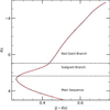 |
Fig. A.1 Example of the polynomial fitting applied to a theoretical isochrone. The black points correspond to the discrete output of the PARSECcode, while the red line represents the polynomial fit used to generate a uniform distribution of points along the sequence. The isochrone shown corresponds to an age of 12.1 Gyr and to the metallicity of the cluster. |
Figure A.1 shows an example of the polynomial fitting applied to a theoretical isochrone. For practical purposes, in sections A.2, A.3 and A.4, “theoretical isochrone” or simply “isochrone” will refer to the uniform array of points generated through this procedure, rather than the original discrete curve.
A.2 Consideration: Fiducial point (FP) and parameterization
To facilitate the comparison between observational data and theoretical isochrones, a FP was defined in the CMD. This is based on the hypothesis that, when the theoretical model is properly fitted to the observed data, there must exist a point on the isochrone that coincides or closely matches the FP within photometric uncertainties. Although an exact correspondence is not always possible due to the discrete nature of both the models and the observations, the FP provides an appropriate initial reference for exploring the E(J − Ks) and  parameter space.
The FP was determined as the average magnitude and color in the CMD region defined by 13.6 < Ks < 13.8 mag and 0.5 < J − Ks < 2.5 mag, resulting in (Ks, J − Ks) = (13.72, 0.92) mag. Fig. 7 shows the position of the FP, marked with a cross.
Once the FP is defined, the difference in magnitude and color between this point and each point of the theoretical isochrone can be computed. These differences represent the E(J − Ks) and  values required to align the isochrone with the observational data, defined as
 (A.2)
where
(A.2)
where  and
and  are the magnitude and color of the i-th point of the theoretical isochrone, while KsFP and (J − Ks)FP correspond to the coordinates of the FP. This yields a set of values
  representing the possible corrections to align the theoretical isochrone with the observations in the CMD. For a discussion of their effects on the determination, see Section A.3.
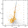 |
Fig. A.2 Same as Fig. 6 , but with overlaid isochrone curves to exemplify the fitting process. The solid blue curve represents the best-fitting isochrone resulting from the complete procedure. The dashed lines illustrate the same theoretical model shifted when choosing different comparison points; the red curve corresponds to a lower E(J − Ks)i value (1.36), while the black curve corresponds to a higher value (1.43) than that obtained for the optimal solution (blue curve). |
Applying these corrections  can be geometrically interpreted as moving the points of the isochrone across the fiducial point. Figure A.2 exemplifies this concept
A.3 Reddening E(J − Ks) and Distance modulus 
The adopted method follows a convergent approach to determine the best combination of parameters describing the stellar cluster. First, the extrinsic parameters E(J − Ks) and  are estimated, followed by the determination of the remaining intrinsic parameter, the age of the cluster, since the metallicity was already established in Section 3.2.
The process begins by selecting an initial set of parameters, including the age of the theoretical isochrone and the previously defined fiducial point. As age is the last parameter to be determined, one of the extremes of the considered range (7 or 14 Gyr) is adopted as a starting point to test convergence toward the same final value regardless of the initial choice.
Then, the values  and E(J − Ks)i are calculated for each point of the theoretical isochrone using Equation A.2. Each pair
  is applied to shift the isochrone in the CMD (see Fig. A.2), resulting in corrected points defined as
 (A.3)
where
(A.3)
where  and
and  correspond to the magnitudes and colors of the shifted isochrone, respectively. For each shift, each observed star is associated with the nearest point of the shifted isochrone, creating groups of stars linked to the same theoretical point. Then, the mean and standard deviation of magnitude and color are computed for each group and compared with the isochrone values through a likelihood function defined as
![Mathematical equation: $M = {{\mathop \sum \nolimits_j \sqrt {{{\left[ {Ks_j^{iso} - \overline {Ks} _j^{obs}} \right]}^2} + {{\left[ {(J - Ks)_j^{iso} - \overline {(J - Ks)} _j^{obs}} \right]}^2}} } \over {\sqrt {\sigma _{\overline {Ks} }^2 + \sigma _{\overline {(J - Ks)} }^2} }},$](/articles/aa/full_html/2026/02/aa56324-25/aa56324-25-eq101.png) (A.4)
where
(A.4)
where  and
and  are the theoretical values of the j-th point of the shifted isochrone;
  and
and  are the observational means of the associated set; and
  and
and  are the standard deviations of the means. The sum extends over the isochrone points with associated observed stars.
This function naturally weights configurations that produce stellar sets with lower dispersion in magnitude and color, giving them greater importance. The goal of this step is to minimize M, which corresponds to maximizing the likelihood of the fit and thus identifying the optimal values  and E(J − Ks)opt. The inner panel of Fig. 7 illustrates the calculation and minimization of M for a 12.1 Gyr isochrone.
An additional aspect to consider is the dependence of the real values of  and E(J − Ks) on the fiducial point. This can be assessed by examining the mean
  at the minimum of M, which indicates the average shift of the observational distribution relative to the isochrone. The final values of
  and E(J − Ks) are thus obtained as
 (A.5)
where δE(J−Ks) corresponds to the mean
(A.5)
where δE(J−Ks) corresponds to the mean  at the minimum of M. Therefore, the choice of the fiducial point is critical to avoid biases in determining the extrinsic parameters. Several points along the RGB were tested, yielding consistent values within the error margins. In this work, we adopted the previously defined FP, which produces δE(J−Ks) values on the order of 0.005 mag, thus minimizing any potential bias.
Finally, the obtained values of µKs and E(J − Ks) allow the calculation of the cluster distance and reddening as described in Section 4.5, providing the essential information to determine the extinction vector used in the cluster age estimation(See Section A.5).
A.4 CMD re-decontamination
To remove stars that were not properly decontaminated in the initial process (see Section 4.3), an additional CMD re-decontamination procedure was implemented. This method relies on the distance of each star to the isochrone shifted by the optimal  and E(J − Ks) values obtained in the previous section. Its goal is to eliminate stars that are too far from the isochrone, as they are likely field contaminants or photometric outliers that could compromise the fitting accuracy.
The procedure applies a 3σ rejection criterion along with a color tolerance radius of 0.2 mag. This threshold was chosen to be wide enough to retain genuine cluster stars but restrictive enough to remove most obvious contaminants. This strategy is particularly effective in mitigating spurious detections, as seen in Fig. 6.
Fig. 7 shows the CMD after applying the re-decontamination process. Removed stars are shown in orange, while retained ones appear in green. The resulting distribution is cleaner and more consistent with the shifted isochrone, indicating that the process effectively reduced the contamination level.
The outcome of this stage is a dataset more representative of the GC population, significantly improving the accuracy of the final age determination.
A.5 Age determination
With the re-decontaminated CMD and using the optimal values of E(J − Ks) and  together with the extinction vector
  computed in Section 4.5, the cluster age was determined.
This process involves iterating over the original set of isochrones obtained from
PARSEC, each with a different age between 7 and 14 Gyr, separated by intervals of 0.1 Gyr. All isochrones are shifted according to the optimal
 and E(J − Ks) values previously determined. For each point of the shifted isochrones, bins oriented along the extinction vector are built, with a length of 0.8 mag along the vector and a width of 0.4 mag in the perpendicular direction.
For each bin, the mean position of the stars in magnitude and color is computed, and then the projected distance between this mean and the corresponding point of the shifted isochrone along the extinction vector is determined as
![Mathematical equation: $\eqalign{ & R = {1 \over N}\sum\limits_{n = 1}^N {\left[ {\left( {K_s^{iso} - K_{s,n}^{iso}} \right){{\left( {{{{A_{{\rm{Ks}}}}} \over {E(J - {K_s})}}} \right)}_{{\rm{Ks}}}}} \right.} \cr & \left. { + \left( {{{(J - {K_s})}^{iso}} - (J - {K_s})_n^{obs}} \right){{\left( {{{{A_{{\rm{Ks}}}}} \over {E(J - {K_s})}}} \right)}_{(J - {K_s})}}} \right] \cr} $](/articles/aa/full_html/2026/02/aa56324-25/aa56324-25-eq118.png) (A.6)
where Ks iso and (J − Ks)iso are the theoretical magnitudes and colors of each point of the shifted isochrone,
(A.6)
where Ks iso and (J − Ks)iso are the theoretical magnitudes and colors of each point of the shifted isochrone,  and
and  are the observed magnitudes and colors of the stars in the bin, N is the number of stars per bin, and
  and
and  are the components of the extinction vector along the magnitude and color directions, respectively.
The residual R quantifies the relative position of the stars with respect to the shifted isochrone. If R > 0, the stars lie below the isochrone along the extinction vector; if R < 0, they lie above, in the opposite direction. The right panel of Fig. 8 exemplifies the calculation of R for isochrones from 7 to 14 Gyr (in 1 Gyr steps) during the convergence iteration. Older ages yield positive R values, indicating that stars lie mostly below the isochrone; conversely, younger ages result in predominantly negative R values. A color cut (J − Ks > 1.8 mag) was also applied to exclude the RGB region, keeping only the subgiant sequence, which is the CMD region most sensitive to age that we were able to sample.
The behavior of R for each shifted isochrone quantifies the quality of the fit between model and observations. Values of R close to zero indicate good alignment between the stars and the isochrone, while larger deviations indicate a poorer fit. Therefore, the absolute mean value residual R,  , is used as the fitting metric. The optimal cluster age corresponds to the minimum of
  , representing the model that best reproduces the observed stellar distribution in the CMD. The left panel of Fig. 8 illustrates the variation in
  as a function of age during the convergence iteration, showing a clear minimum around 12.1 Gyr.
Once the age minimizing  is identified, the entire procedure is repeated starting the iteration with the corresponding isochrone to recompute new optimal values of E(J − Ks) and
  . This iterative process continues until the parameters converge to stable values, i.e., when they no longer change significantly between consecutive iterations.
To test the robustness of the method, the fitting was repeated starting from both extremes of the age range (7 and 14 Gyr). In both cases, the algorithm converged to the same final values of age, E(J − Ks), and  , confirming the consistency and reliability of the approach.
The final values of the parameters derived from this method are reported in Section 4.4 of the main article, where the error analysis and astrophysical implications are discussed in detail.
Appendix B Cluster’s orbital properties: Additional information
We updated the orbital calculator software DELOREAN (Blaña et al. 2020) with new gravitational potentials for the Milk Way (Blaña et al. in prep.). The circular velocity profiles of the potential are shown in Fig.B.1. For the MW’s box/peanut bulge, flat bar, and inner disk potential we used the stellar mass density analytical model of S22 which was derived from made-to-measure orbital models fitted to MW 3D observations (Portail et al. 2017; Wegg & Gerhard 2013).
As this model traces well the stellar mass distribution within 15 kpc, we used it to obtain the gravitational potential by solving the Poisson equation with the Fast Fourier Transform method. We also adopted the bar pattern speed of Ωbar = 39.0± 3.5 km s−1 kpc−1 rad (Portail et al. 2017), and a bar angle of 27 deg(Wegg & Gerhard 2013) which encompasses other estimates in the literature within the errors. We also included the potentials of other mass components with mass and scale length estimates based on BG16. These are the nuclear components, which include the Sagittarius A∗ supermassive black hole modeled with a Plummer profile (SMBH: M•= 4.3×10⁶ M⊙ and a softening of rpl = 1.6 pc), the nuclear star cluster (NSC: MNSC = 1.8×10⁷ M⊙ and half-mass radius rpl = 4.2pc), and the nuclear stellar disk modeled with a Miyamoto-Nagai profile (NSD: MNSD = 1.4×10⁹ M⊙ and scale length and height of Rd = 90 pc and zh =45 pc, respectively). The cold gaseous disk (atomic and molecular gas) is also modeled with a Miyamoto-Nagai profile with a mass of Mgas = 7×10⁹ M⊙ and scale length and height of Rd = 2.6 kpc and zh = 0.3 kpc, respectively. For the dark matter halo we also use the Navarro-Frenk-White (NFW) profile adapted from BG16 with a virial mass of Mvir = 1.3×10¹² M⊙ and concentration of c = 16 which fits well the gas rotation curve and the circular velocity at the Sun’s location (see Fig.B.1). We note that the hot gas and stellar halo mass contributions are smaller than the dark-halo error estimates, and therefore omitted. We used Fourier analysis to determine the typical orbital periods of the cluster, finding values around Tϕ ∼ 100 Myr, allowing us to adopt a time step of dt = 0.1 Myr to ensure enough precision while allowing faster computations.
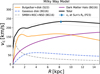 |
Fig. B.1 Circular velocity profiles (vc) for the MW potential model used here (black curve), and its components. We show vc for the stellar bar and inner disk model of S22 (orange). The additional components are derived from BG16 which are: the gaseous disk (blue), the nuclear components (gray) corresponding to the Sagittarius A* super massive black hole (SMBH), the nuclear star cluster (NSC), and the nuclear stellar disk (NSD), and the dark matter halo. More details in §B. We include the vc at Sun’s position vc =233±7 km/s (Põder et al. 2023) at its galactocentric distance R0 =8.2±0.1 kpc BG16. We include the axisymmetric MW potential MWPotential2014 from Bovy (2015) (gray dotted line) to compare the gravitational potential differences with our barred MW model. |
All Tables
All Figures
|
Fig. 1 False-color composite image using the infrared J (blue) and Ks (red) bands, centered on the GC VVV-CL001. The red dashed circle marks the core radius (rc = 0.′94), while the cross indicates the cluster’s central position. |
| In the text | |
|
Fig. 2 Left panel: CMD of the VVV sources within 5′ of the cluster center with (red dots) and without (black dots) PMs from the Gaia catalog. Right panel: comparison of PMs in Galactic coordinates from Gaia and VVV. The red line indicates the fit of the data with a linear relation of unit slope. |
| In the text | |
|
Fig. 3 Decontaminated VVV CMD of VVV-CL001. All sources detected within 1′ from the cluster center are shown as gray dots. Spectroscopic targets are marked as large colored points: blue, cyan, green and purple symbols are stars rejected as cluster members because they have a discrepant distance to the cluster center, mean RV, metallicity, and PMs, respectively. Red points represent spectroscopically confirmed cluster members. |
| In the text | |
|
Fig. 4 Upper panel: RV of the spectroscopic targets as a function of distance from the cluster center. The horizontal lines represent our velocity cuts (±15 km s−1). Middle panel: metallicity of the spectroscopic targets as a function of distance from the cluster center. The horizontal lines represent our metallicity cuts (±0.20 dex). For both panels the color-coding is the same as in Fig. 3. Lower panel: radial density profile of the photometric sources with respect to the cluster center. The dotted curve indicates the best fit of a King (1962) radial profile. |
| In the text | |
|
Fig. 5 PM plane for cluster VVV-CL001.The gray points stand for stars from the Gaia DR3 catalogue and the large colored points represent our spectroscopic targets. The color-coding is the same as in Fig. 3. |
| In the text | |
|
Fig. 6 CMD of the photometry obtained in the VVV CL001 field within a radius of 0.′94 from the center of the cluster (gray points). The orange points are the stars resulting from the statistical decontamination process. The black symbols give the average photometric errors per magnitude bin. |
| In the text | |
|
Fig. 7 CMD of VVV-CL001. The green points represent stars retained after the re-decontamination process, while the orange points indicate the rejected stars. The red points correspond to CaT-confirmed members of VVV-CL001. The black cross marks the adopted fiducial point, and the blue curve shows the best-fitting theoretical isochrone. Inset: value of the metric M (Eq. (A.4)) for each tested combination of E(J − Ks) and |
| In the text | |
|
Fig. 8 Left panel: mean absolute residual |
| In the text | |
|
Fig. 9 Left panel: Color–Color diagram. Green points: only RGB stars from the photometric data resulting from statistical decontamination. Blue points: best-fit isochrone model from Section 4.4. The green and blue dotted curves show the linear fit of the green and blue points, respectively. Right panel: plane of |
| In the text | |
|
Fig. 10 Orbital calculations for VVV-CL001. We show the most likely current position (large orange circle) and the corresponding orbit (white curve) showing its past −150 Myr orbit (solid) and future 150 Myr orbit (dashed) seen in the X −Y plane view (top panel) and the X −Z view (bottom panel). To avoid crowding we show a subsample of 20 randomly selected orbits from the total of 104 orbits, giving their current positions (smaller circles), their past orbits (green) and future orbits (purple). The density probability (color map) shows the regions that the orbits inhabit. The stellar surface mass density contours of the MW bar and inner disk model of S22 reveal that this cluster lives between the inner disk and the bulge–bar region. We also plot the Sun’s position. We note that in this frame the MW and the bar rotate clockwise, with the bar havings a rotation period of Tbar =157 Myr. |
| In the text | |
|
Fig. A.1 Example of the polynomial fitting applied to a theoretical isochrone. The black points correspond to the discrete output of the PARSECcode, while the red line represents the polynomial fit used to generate a uniform distribution of points along the sequence. The isochrone shown corresponds to an age of 12.1 Gyr and to the metallicity of the cluster. |
| In the text | |
|
Fig. A.2 Same as Fig. 6 , but with overlaid isochrone curves to exemplify the fitting process. The solid blue curve represents the best-fitting isochrone resulting from the complete procedure. The dashed lines illustrate the same theoretical model shifted when choosing different comparison points; the red curve corresponds to a lower E(J − Ks)i value (1.36), while the black curve corresponds to a higher value (1.43) than that obtained for the optimal solution (blue curve). |
| In the text | |
|
Fig. B.1 Circular velocity profiles (vc) for the MW potential model used here (black curve), and its components. We show vc for the stellar bar and inner disk model of S22 (orange). The additional components are derived from BG16 which are: the gaseous disk (blue), the nuclear components (gray) corresponding to the Sagittarius A* super massive black hole (SMBH), the nuclear star cluster (NSC), and the nuclear stellar disk (NSD), and the dark matter halo. More details in §B. We include the vc at Sun’s position vc =233±7 km/s (Põder et al. 2023) at its galactocentric distance R0 =8.2±0.1 kpc BG16. We include the axisymmetric MW potential MWPotential2014 from Bovy (2015) (gray dotted line) to compare the gravitational potential differences with our barred MW model. |
| In the text | |
Current usage metrics show cumulative count of Article Views (full-text article views including HTML views, PDF and ePub downloads, according to the available data) and Abstracts Views on Vision4Press platform.
Data correspond to usage on the plateform after 2015. The current usage metrics is available 48-96 hours after online publication and is updated daily on week days.
Initial download of the metrics may take a while.