| Issue |
A&A
Volume 706, February 2026
|
|
|---|---|---|
| Article Number | A84 | |
| Number of page(s) | 29 | |
| Section | Interstellar and circumstellar matter | |
| DOI | https://doi.org/10.1051/0004-6361/202556371 | |
| Published online | 06 February 2026 | |
Resolution and calibration effects in high contrast polarimetric imaging of circumstellar scattering regions
1
ETH Zurich, Institute for Particle Physics and Astrophysics,
Wolfgang-Pauli-Strasse 27,
8093
Zurich,
Switzerland
2
Univ. Grenoble Alpes, CNRS, IPAG,
38000
Grenoble,
France
★ Corresponding author: This email address is being protected from spambots. You need JavaScript enabled to view it.
Received:
11
July
2025
Accepted:
20
November
2025
Abstract
Context. Many circumstellar dust scattering regions have been detected and investigated with polarimetric imaging. However, the quantitative determination of the intrinsic polarization and of dust properties is difficult because of complex observational effects.
Aims. This work investigates the instrumental convolution and polarimetric calibration effects for high contrast imaging polarimetry with the aim of defining the measuring parameters and calibration procedures for accurate measurements of the circumstellar polarization.
Methods. We simulated the instrumental convolution and polarimetric cancellation effects for two axisymmetric point spread functions (PSFs), a Gaussian PSFG and an extended PSFAO, typical for a modern adaptive optics system. The PSFs have the same diameter DPSF for the PSF peak. Further, polarimetric zero-point corrections (zp-corrections) were simulated for different cases, including coronagraphic observations and systems with barely resolved circumstellar scattering regions.
Results. The PSF convolution reduces the integrated azimuthal polarization, ΣQϕ, for the scattering region, while the net Stokes signals ΣQ and ΣU are not changed. For non-axisymmetric systems, a spurious Uϕ signal is introduced by the convolution. These effects are strong for compact systems and for the convolution with an extended PSFAO. Compact scattering regions can be detected down to an inner working angle of r ≈ DPSF based on the presence of a net ΣQϕ signal. Unresolved central scattering regions can introduce a central Stokes Q, U signal that can be used to constrain the scattering geometry even at separations r < DPSF. The smearing by the halo of the PSFAO produces an extended, low surface brightness polarization signal. These effects change the angular distribution of the azimuthal polarization, Qϕ(ϕ), but the initial Qϕ′(ϕ) signal can be partly recovered with the analysis of measured Stokes Q and U quadrant pattern. We find that applying a polarimetric zp-correction for the removal of offsets from instrumental or interstellar polarization depends on the selected reference region and can introduce strong bias effects for ΣQ and ΣU and the azimuthal distribution of Qϕ(ϕ). Strategies for the zp-correction are described for different data types, such as coronagraphic data or observations of partly unresolved systems. These procedures provide polarization parameters that can be easily reproduced with model simulations.
Conclusions. The simulations describe the impact of the PSF convolution and of calibration offsets for imaging polarimetry in a systematic way, and they show when these effects are strong and how they can be considered in the analysis. This defines also suitable measuring parameters and procedures for the quantitative characterization of the intrinsic scattering polarization Qϕ′ for an accurate determination of the properties of the circumstellar dust.
Key words: scattering / instrumentation: high angular resolution / techniques: polarimetric / protoplanetary disks / circumstellar matter, dust / extinction
© The Authors 2026
 Open Access article, published by EDP Sciences, under the terms of the Creative Commons Attribution License (https://creativecommons.org/licenses/by/4.0), which permits unrestricted use, distribution, and reproduction in any medium, provided the original work is properly cited.
This article is published in open access under the Subscribe to Open model. This email address is being protected from spambots. You need JavaScript enabled to view it. to support open access publication.
1 Introduction
Dust in circumstellar disks around young stars and dust in shells around red giants have been recognized in many systems as infrared excess in the spectral energy distribution. This dust plays an important role in the formation of stars and planetary systems (Birnstiel 2024) and the mass loss of evolved stars and the dust enrichment of the interstellar medium (Ferrarotti & Gail 2006).
In the past decade, a lot of new information on circumstellar dust has been obtained with imaging observations of scattered stellar light in the near-IR and visual wavelength range. High-contrast instruments at large ground-based telescopes achieve an angular resolution of up to 20 mas, and this provides important information about the geometric distribution and the scattering properties of the circumstellar dust. In particular, the new information from scattered light observations is complementary to the extensive data already available from IR observations of the thermal emission of the dust around protoplanetary disks (e.g., Woitke et al. 2019), debris disks (e.g., Hughes et al. 2018; Chen et al. 2014), and red giants (e.g., Höfner & Olofsson 2018).
The determination of the geometric structure and the scattering properties of circumstellar dust near stars is of much interest for the investigation of the formation of planetary systems from dusty circumstellar disks around young stars. The measurement of circumstellar polarization is also important for the study of dust formation in the winds around cool, mass loosing stars. However, detection of the scattered intensity from circumstellar dust is difficult because the signal is faint and often hidden in the strong glare of the central star. This requires a careful separation of the stellar signal from the circumstellar signal, which can be achieved with high contrast techniques using space telescopes, such as the Hubble Space Telescope (HST; e.g., Kalas et al. 2013; Schneider et al. 2014; Zhou et al. 2023) or JWST (e.g., Gáspár et al. 2023; Lawson et al. 2023), or with ground-based telescopes using adaptive optics (AO) systems (Milli et al. 2017; Ren et al. 2023).
High-resolution imaging polarimetry is a very powerful method to separate the circumstellar polarization signal introduced by dust scattering from the direct light of a bright central source, which usually has no or only a small net linear polarization (e.g., Kuhn et al. 2001; Quanz et al. 2011). Great progress has been achieved with new instruments for imaging polarimetry in combination with AO systems at large ground-based telescopes, including Subaru CIAO, HiCIAO, and SCeXAO instruments (Murakawa et al. 2004; Hodapp et al. 2008; Lucas et al. 2024); Gemini GPI (Perrin et al. 2015); and VLT NACO and SPHERE (Lenzen et al. 2003; Beuzit et al. 2019). Polarimetric imaging of many objects has been obtained, including protoplanetary disks (e.g., Avenhaus et al. 2018; Benisty et al. 2023, and references therein), debris disks (e.g., Esposito et al. 2020; Crotts et al. 2024), circumstellar shells around red giants (e.g., Ohnaka et al. 2016; Khouri et al. 2020; Montargès et al. 2023), and post-AGB stars (e.g., Andrych et al. 2023).
High-resolution imaging polarimetry is a quite new and not so simple observing technique because of point spread function (PSF) smearing and polarization cancellation effects and noise in the weak differential signal (Schmid et al. 2006; Schmid 2022). In addition the polarimetric calibration of the complex high contrast imaging systems has to be considered (e.g., Tinbergen 2007; Schmid et al. 2018; de Boer et al. 2020; van Holstein et al. 2020), including the temporal PSF variations for ground-based observations using AO systems (Tschudi & Schmid 2021; Ma et al. 2023). Depite this, many impressive results on dust scattering geometry have been obtained, but for most objects, no detailed analysis of the polarized intensity has been attempted, mostly because this was not the focus of the study. For some special cases, the polarized flux is derived more accurately to constrain the properties of the scattering dust, for example, for extended circumstellar disks (Stolker et al. 2016; Monnier et al. 2019; Milli et al. 2019; Arriaga et al. 2020; Hunziker et al. 2021), axisymmetric systems (Pinilla et al. 2018; Tschudi & Schmid 2021; Ma et al. 2023), and edge-on debris disks (e.g., Graham et al. 2007; Engler et al. 2017). It is highly desirable that such detailed studies on the circumstellar polarization are applied to a larger sample and are further improved for some key objects.
Accurate polarimetric measurements for circumstellar scattering regions require a good understanding of the observational aspects. Convolution effects degrade the measurable polarization signal, as described for some cases in Schmid et al. (2006), Avenhaus et al. (2017), Heikamp & Keller (2019), Tschudi & Schmid (2021), and Ma et al. (2023, 2024b). Additional issues are polarization offsets introduced by instrumental effects, interstellar polarization, and an intrinsically polarized central star. These offsets can be eliminated with a polarimetric normalization, which sets the polarization for a certain region to zero (Quanz et al. 2011; Avenhaus et al. 2014). We call this procedure hereafter polarimetric zero-point correction (zp-correction).
A very useful and frequently used way to describe the circumstellar signal is the azimuthal polarization Qϕ (Schmid et al. 2006; Quanz et al. 2013). A convolution or an offset by a zp-correction introduces for Qϕ quite complex changes, and some of these effects have not been described in detail or have not been investigated at all. For example, it is clear that polarimetric offsets, or a zp-correction, change the polarization signal, but this work describes for the first time how this change affects the azimuthal distribution of the circumstellar Qϕ signal. Because of the lack of a systematic study, it is difficult to extrapolate findings from the papers cited above to a more general picture.
For compact scattering regions near the star, the mentioned effects are much stronger, and they must even be considered for a qualitative interpretation of the polarization signal. Therefore, the scattering regions at small separations to the star of r ≲ 5 λ/D, or r ≲ 200 mas for large telescopes with AO systems, are often disregarded despite the fact that these regions are scientifically very interesting. They correspond for protoplanetary disks at ≈ 100 pc to the innermost <20 AU, which is where planets form (e.g., Birnstiel 2024), and for nearby red giant stars, they correspond to a separation of a few stellar radii where dust particles condensate (e.g., Höfner & Olofsson 2018). In non-coronagraphic and non-saturated data, this region is sometimes masked in the data reduction process because it looks “noisy” or shows an unexplained polarization pattern. However, these features might just be caused by a polarization offset or a convolution effect.
In coronagraphic observations, the central region is hidden behind the focal plane mask to achieve observations more sensitive to the polarization signal further out. Also for this type of data, it is important to understand the impact of the convolution and of polarization offsets.
This work presents model simulations and a parameter framework for a systematic description of the PSF convolution effects and an investigation of the polarimetric offsets introduced by the instrument, the interstellar polarization, the central star, or by the zp-correction applied to the data. The results should provide a better understanding of these effects for the interpretation of observational results and be useful for the definition of observing and measuring strategies for polarimetric imaging of circumstellar scattering regions.
This paper is organized as follows. In the next section, we describe the model simulation and introduce the used polarimetric parameters. Section 3 describes the degradation of the scattering polarization by the PSF convolution for axisymmetric circumstellar scattering regions and for inclined disk models. The polarimetric calibration and zp-correction effects are investigated in Sect. 4 and discussed in particular for coronagraphic observation and for data with only partially resolved circum-stellar scattering regions. In Sect. 5 the results are summarized and discussed in the context of observational data. Detailed information, in particular numerical results for the presented simulations, are given in the appendix.
2 Model calculations
The block diagram in Fig. 1 gives an overview of the steps involved in imaging polarimetry using the Stokes Q = I0 − I90 and U = I45 − I135 polarization parameters as example. The full process is described by the boxes connected with red arrows, from the intrinsic polarization model defined in system coordinates Q′(x, y), U′(x, y) to the model in sky coordinates Q′(α, δ), U′(α, δ), including the contribution of interstellar polarization Q″(α, δ), U″(α, δ), to the observed signal Q(α, δ), U(α, δ) and the result after a possible polarimetric zp-correction Qz(α, δ), Uz(α, δ). This is simplified in the simulations according to the blue path in Fig. 1 by calculating the observed polarization signal in system coordinates Q(x, y), U(x, y) considering only convolution and polarimetric offsets and a zp-correction Qz(x, y), Uz(x, y) for the calibration of the data. This approach still considers many of the key aspects of polarimetric imaging but disregards second-order effects and particular problems of individual instruments or datasets. The parameters for the x, y coordinates are used for the description of the model simulations the x, y coordinates, while some general polarimetric principle are discussed for on sky parameters using (α, δ) coordinates. However, it is important to be aware of simplifying assumptions outlined in Fig. 1 for the interpretation of the model results.
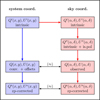 |
Fig. 1 Block diagram with the simplified description of the simulated imaging polarimetry given in blue. The red arrows show the full imaging process from the intrinsic model to the on-sky model including interstellar polarization to the observed and possibly zp-corrected polarization signal. |
2.1 Intrinsic scattering models
The intrinsic models for the circumstellar dust scattering region and a point-like central star at x0, y0 are described by 2D maps for each component of the Stokes vector
 (1)
(1)
The components describe the intensity, I′(x, y), and the linear polarization, Q′(x, y), U′(x, y), in x,y coordinates aligned with the object. The circular polarization signal V′ is expected to be much weaker for circumstellar scattering and is neglected. In principle, multiple scattering by dust can produce a circular polarization signal, in particular for (magnetically) aligned dust grains. Measurements for circumstellar circular polarization exist since many decades (e.g., Kwon et al. 2014; Bastien et al. 1989; Angel & Martin 1973), but the signals are weak, or originate from regions far away from the star, where interstellar magnetic fields may play a role. Considering this in our models is beyond the scope of this paper.
The models use  consisting of a star,
  , with or without an intrinsic polarization,
  ,
,  , and an extended dust scattering region,
  , according to the vector components
 (2)
(2)
 (3)
(3)
 (4)
(4)
In most models the star is not polarized and  and
and  are set to zero or
  and
and  .
.
Scattering geometries. We considered the axisymmetric models Ring0 and Disk0 representing circumstellar disks seen pole-on or spherical dust shells as illustrated by the intensity maps  in the upper row of Fig. 2. The intrinsic polarization flux,
  , is proportional to the intensity,
  .
.
The Ring0 models have a mean radius, r0, and a Gaussian radial profile with full width at half maximum (FWHM) of ∆r = 0.2 r0, and r0 is varied from 3.15 to 806.4 mas. The Disk0 models are axisymmetric scattering regions extending from an inner radius, rin, to an outer radius, rout, with a surface brightness described by the power law
 (5)
with reference radius rref. Three cases, Disk0α0, Disk0α−1, and Disk0α−2, are considered with α = 0 for a constant surface brightness and α = −1 and −2 for a brightness decreasing with distance. For all cases the outer radius is rout = 100.8 mas while the radius of the inner cavity is varied between rin = 3.15 mas and 50.4 mas to investigate the differences between fully resolved and partially resolved scattering regions. Figure 2 shows
(5)
with reference radius rref. Three cases, Disk0α0, Disk0α−1, and Disk0α−2, are considered with α = 0 for a constant surface brightness and α = −1 and −2 for a brightness decreasing with distance. For all cases the outer radius is rout = 100.8 mas while the radius of the inner cavity is varied between rin = 3.15 mas and 50.4 mas to investigate the differences between fully resolved and partially resolved scattering regions. Figure 2 shows  maps for Disk0α−1 with rin = 12.6 mas and 50.4 mas.
Simulations for non-axisymmetric scattering geometries are obtained by adopting the Ring0 and Disk0 geometries for inclined, flat disks with i = 60◦. The dust density in the disk plane ρd(rd) of the inclined models RingI60 and DiskI60α0, DiskI60α−1, DiskI60α−2 are described by the same radial parameters as for the axisymmetric models. The scattering angle in the inclined disk model varies as a function of azimuthal angle ϕ on the disk, and therefore the scattered intensity and polarization also depend on ϕ. This is simulated as in Schmid (2021) for flat, optically thin disks with a dust scattering phase function described by a Henyey-Greenstein function for the intensity with asymmetry parameter g = 0.6 and a Rayleigh scattering like dependence for the fractional polarization with pmax = 0.25. With these settings the resulting model maps I′(x, y) depend only on r0 for the RingI60 model and on α and the radius of the central cavity rin for the DiskI60 models. Figure 2 shows the maps for RingI60 and DiskI60α−1 with the same r0 and rin parameters as for the pole-on models. The major and minor axes of the inclined disks are aligned with the x and y coordinates and the backside of the disk is in the +y direction. Because of the strong forward scattering (g = 0.6) the intensity signal is enhanced on the front-side, and this is a frequently observed property for inclined disks (e.g., Ginski et al. 2023).
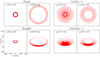 |
Fig. 2 Maps for the intrinsic disk intensity |

2.2 Sky coordinates and interstellar polarization
Observations are obtained in sky coordinates (α, δ) and the intrinsic maps in system coordinates Q′(x, y), U′(x, y) can be transformed into the sky coordinates Q′(α, δ), U′(α, δ) by a rotation of the geometry and the polarization vector (e.g., Schmid 2021). The signal reaching Earth Q″(α, δ), U″(α, δ) is often affected by interstellar polarization introduced by dichroic absorption of magnetically aligned interstellar grains (e.g., Draine 2003). This introduces a fractional polarization offset, which can be described for the usual low-polarization case (Q′, U′ ≪ I′ and q, u ≪ 1) by
 (6)
(6)
 (7)
where qis, uis are the components of the fractional interstellar polarization
(7)
where qis, uis are the components of the fractional interstellar polarization  with position angle θis = 0.5 · atan2(uis, qis)1 defined in sky coordinates. We used flux ratios to quantify the resulting intensity or polarization so that the interstellar transmission losses can be neglected. Extreme dichroic extinction by the interstellar medium can convert linear polarization partly to circular polarization (e.g., Kwon et al. 2014), but this is not considered in this work.
2.3 Signal degradation by ground-based AO observations
The turbulence in the Earth atmosphere leads to a strong seeing convolution of the incoming signal (I″, Q″, U″). With an AO system the seeing can be strongly reduced but there remain smearing and polarimetric cancellation effects that can strongly change the spatial distribution of the observed signal I(α, δ), Q(α, δ), U(α, δ) when compared to the incoming signal (e.g., Perrin et al. 2003; Fétick et al. 2019). The effects are particularly strong for not well resolved structures near the star. The AO correction depends on the atmospheric turbulence and instrument properties, and therefore the observational PSF changes with time and shows various types of non-axisymmetric structures (e.g., Cantalloube et al. 2019). In addition, AO instruments are complex and they usually introduce instrumental polarization offsets which are difficult to calibrate accurately (Tinbergen 2007). These observational effects are investigated in this work.
PSF convolution. Axisymmetric PSFs are adopted so that the convolved scattering signal does not depend on the orientation of the observed system. Therefore we can apply the convolution directly to the models described in disk coordinates (x, y). Real PSFs are variable and deviate from axisymmetry but assuming a stable, axisymmetric PSF is a reasonable approximation for PSFs with high Strehl ratio or for the averaged PSF obtained after a number of polarimetric cycles taken in field rotation mode.
We used PSFAO(x, y) representing an AO system with a narrow core with FWHM or diameter of DPSF = 25.2 mas and an extended halo. This profile is obtained by averaging azimuthally the PSF described in Schmid et al. (2018) for the standard star HD 161096 taken under excellent condition with the AO instrument VLT/SPHERE/ZIMPOL in the N_I filter (λc = 817 nm) with a Strehl ratio of about 0.4. The radial profile of PSFAO is plotted in Fig. 3 together with a Gaussian profile PSFG with the same diameter DPSF, which is used to investigate the impact of the extended halo in PSFAO on the convolved signal. Convolution with a Gaussion PSF with DPSF ≈ λ/D could also represent roughly diffraction limited imaging polarimetry with a space telescope with diameter D or ground based seeing limited imaging polarimetry with DPSF of the order ≈1000 mas.
Polarimetric calibration. Many types of instrumental effects are introduced in observations taken with high-contrast imaging polarimetry and there exist established procedures to calibrate the data, for example for SPHERE/IRDIS (de Boer et al. 2020; van Holstein et al. 2020) and SPHERE/ZIMPOL polarimetry (Schmid et al. 2018; Hunziker et al. 2020; Tschudi et al. 2024). Individual instruments show also particular effects but these aspects are beyond the scope of this paper.
A very general and important observational effect are the offsets introduced by the interstellar pis or by the instrument polarization pinst of the kind described in Eqs. (6) and (7). Because the intensity of the star ΣIs is much higher than the polarization from the circumstellar dust ΣQd, ΣUd, by about a factor 100 or even more, already a small fractional polarization offset for the central star of about p ≈ 0.001 can strongly disturb the circumstellar signal, while p ≈ 0.01 can completely mask that signal. In addition, there could also be a contribution from an intrinsic polarization of the central star. The effects of polarimetric offsets do not depend on the orientation of the selected coordinate system, and therefore they can also be treated in the (x, y) coordinate system.
Unfortunately, it can be quite difficult to disentangle the different contributions to the overall polarimetric offset, and therefore an ad hoc zp-correction for the polarization is often applied to the data based on the assumption that the polarization of the target in a selected integration region is zero, or at least very small (Quanz et al. 2011; Avenhaus et al. 2014). A polarimetric offset sets the integrated Stokes parameters in a certain region to zero ΣQz = ∫ Qz(α, δ)dαdδ = 0 and similar for ΣUz = 0, but this procedure can introduce a bias. For coronagraphic observations, the central star cannot be included for the determination of the zp-correction, and this adds another complication, which we also describe later in the text.
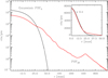 |
Fig. 3 Radial profiles for the extended PSFAO (red) and the Gaussian PSFG (black). In the main panel, the total flux is normalized to 106 counts. In the inset, PSFG is reduced by a factor of 0.4 for a comparison of the PSF cores. The pixel size is 3.6 mas × 3.6 mas. |
2.4 Analysis of diagnostic polarization parameters
The impact of the convolution and the polarimetric zp-correction, follows from the comparisons between the simulated observational maps I(x, y), Q(x, y), U(x, y) or the corresponding zp-corrected polarization Qz(x, y), Uz(x, y) with the initial maps I′(x, y), Q′(x, y), U′(x, y).
Circumstellar scattering produces predominantly a linear polarization in azimuthal direction Qϕ with respect to the central star located at x0, y0. Therefore Qϕ is a very useful polarization parameter which is defined by
 (8)
(8)
 (9)
with ϕxy = atan2((x − x0), (y − y0)) according to the description of Schmid et al. (2006) for the radial Stokes parameters Qr, Ur and using Qϕ = −Qr and Uϕ = −Ur. The Uϕ(x, y) parameter gives the linear polarization component rotated by 45◦ with respect to azimuthal component Qϕ(x, y). The different polarized intensities for a given point (x, y) in the polarization maps are related to the polarized flux for the linear polarization according to
(9)
with ϕxy = atan2((x − x0), (y − y0)) according to the description of Schmid et al. (2006) for the radial Stokes parameters Qr, Ur and using Qϕ = −Qr and Uϕ = −Ur. The Uϕ(x, y) parameter gives the linear polarization component rotated by 45◦ with respect to azimuthal component Qϕ(x, y). The different polarized intensities for a given point (x, y) in the polarization maps are related to the polarized flux for the linear polarization according to
 (10)
(10)
Figure 4 illustrates the relation between Qϕ and the Stokes parameters Q and U for a pole-on disk ring. In this model the Uϕ component is zero and P(x, y) = Qϕ(x, y) because of the axisymmetric geometry. Non-axisymmetric geometries can produce an intrinsic  signal, for example by multiple scattering (Canovas et al. 2015), but for the simple (single scattering) models adopted in this work the intrinsic
  -signal is also zero for inclined disks. However, the convolution and polarimetric offsets will introduce also for these models a Uϕ signal, which is equivalent to a non-azimuthal polarization component (Fig. 9).
The observational Q(x, y), U(x, y) or Qϕ(x, y), Uϕ(x, y) maps have in high contrast imaging polarimetry often a lower signal per pixel than the photon noise σ(x, y) or other pixel to pixel noise sources. Therefore, the polarized flux P(x, y) is biased, because it is always positive, and the measured values follow a Rice probability distribution. For a low polarization P(x, y) ≲ σ(x, y) the noise will introduce on average a signal of about P(x, y) ≈ +σ(x, y) (Simmons & Stewart 1985), and this can add up to a very significant spurious signal for the polarized flux ΣP in an integration region Σ containing many tens or more pixels. This noise problem is avoided by using Qϕ(x, y) for measuring the strength of the spatially resolved linear polarization (Schmid et al. 2006). This is a reasonable approximation, because circumstellar scattering produces predominantly a polarization in azimuthal direction with Qϕ(x, y) ≫ 0 and Uϕ(x, y) ≈ 0, and therefore one can consider Qϕ as rough proxy for P according to
 (11)
(11)
Enhanced random noise in the data does not change the mean Qϕ signal for a pixel region, but P is for observational data often very significantly affected by the bias problem described above. The simulations in this work do not consider statistical noise in the data. However, there are other systematic differences between Qϕ(x, y) and P(x, y) because of the Uϕ(x, y) signal introduced by the PSF convolution and polarization offsets, which are described by the simulation results.
The convolution and zp-correction effects are quantified using polarization parameters integrated in well-defined apertures
 (12)
where X is a place holder for the PSF convolved radiation parameters, such as X = {I, Q, U, P, Qϕ, Uϕ}, and similarly for X′ or Xz for the intrinsic models or zp-correcected models, respectively. The term Σ defines a circular aperture centered on the star for the determination of the system integrated parameters. Later, we also consider other axisymmetric circular and annular apertures for the parameters of radial subregions (see Sect. 4.3.1). Axisymmetric apertures are very useful for quantifying the convolution by an axisymmetric PSF and polarization offsets for an intensity signal dominated by the axisymmetric stellar PSF. An overview on the used polarization parameters is given in Appendix A (Tables A.1 and A.2).
(12)
where X is a place holder for the PSF convolved radiation parameters, such as X = {I, Q, U, P, Qϕ, Uϕ}, and similarly for X′ or Xz for the intrinsic models or zp-correcected models, respectively. The term Σ defines a circular aperture centered on the star for the determination of the system integrated parameters. Later, we also consider other axisymmetric circular and annular apertures for the parameters of radial subregions (see Sect. 4.3.1). Axisymmetric apertures are very useful for quantifying the convolution by an axisymmetric PSF and polarization offsets for an intensity signal dominated by the axisymmetric stellar PSF. An overview on the used polarization parameters is given in Appendix A (Tables A.1 and A.2).
For a given integration region, Σ, an “aperture” polarization, (Σ) = (ΣQ)2 + (ΣU)2)1/2. with the corresponding position angle θ(Σi) can be defined in the same way as for aperture polarimetry. These parameters are useful for specifying the polarization of the star or the fractional polarization p = (Σ)/ΣI and the fractional Stokes parameters q, u in order to quantify polarization offsets and zp-correction factors (see Appendix A).
The polarization parameters are usually normalized to the integrated intrinsic polarization  , such as
  ,
,  , because
  provides a good reference for the characterization of the impact of the convolution or of offsets on polarization parameters.
For the characterization of the azimuthal distribution of the polarization Q(ϕ) and U(ϕ), the four Stokes Q quadrants, Qxxx = {Q000, Q090, Q180, Q270}, and the four Stokes U quadrants, Uxxx = {U045, U135, U225, U315}, are used (Schmid 2021), while Xxxx stands for all eight parameters. They represent the Stokes Q and U polarization in the four wedges of 90◦ centered on the position angle ϕ = xxx, which form for well-resolved circum-stellar scattering regions the positive-negative Q and U quadrant patterns. The signals in these quadrants are changed by the convolution and polarization offsets, and they are useful to quantify the corresponding changes for the azimuthal distribution of the polarization signal Qϕ(ϕ).
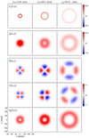 |
Fig. 4 Maps for the Ring0 models with r0 = 12.6 mas (left), 25.2 mas (middle), and 50.4 mas (right) for the intrinsic circumstellar intensities, |


3 Polarization degradation by the PSF convolution
This section describes the basic PSF smearing and cancellation effects for imaging polarimetry of circumstellar scattering regions. The convolution is always applied to the intrinsic intensity I′ and Stokes Q′, U′ maps, or from maps with a polarization offset like the Q″, U″ maps, and from the resulting Q and U one can then derive according to Eq. (8)–(10) the convolved maps for the polarization parameters Qϕ, Uϕ and P (e.g., Tschudi & Schmid 2021). Alternatively, one could also apply the convolution to the  ,
,  ,
,  , and
, and  polarization components and derive from this the convolved intensity and polarization maps, because the convolution operation is distributive (PSF ∗ A + PSF ∗ B = PSF ∗ (A + B)). However, a direct convolution of the intrinsic azimuthal polarization (
 ) or of the polarized flux (PSF ∗ P′) gives wrong results.
3.1 Convolution for axisymmetric scattering models
3.1.1 Narrow pole-on rings
The convolution depends strongly on the spatial resolution, specifically on the angular size of the scattering signal compared to the PSF widths. This can be described by an axisymmetric scattering geometry like for a dust disk seen pole-on or a spherical dust shell.
Simulations for the convolution of the Ring0 models are shown in Fig. 4 for three ring sizes with r0 = 12.6, 25.2, and 50.4 mas and using the Gaussian PSFG. Maps for the intrinsic dust scattering intensities  , and convolved intensities Id(x, y) and the polarization Qd(x, y), Ud(x, y), Qϕ,d(x, y) are given. The central star is unpolarized in this model and there is Qd = Q, Ud = U and Qϕ,d = Qϕ. All three models have the same intrinsic flux
  and
and  , and therefore the peak fluxes scale as max
  and are higher for a smaller r0. The star is unpolarized and therefore does not contribute to the polarization maps. The star Is is not included in the intensity maps because for realistic cases it would dominate strongly the scattering intensity Id. For the intrinsic model there is
  and
and  . For axisymmetric models, this property is not changed by the convolution, and therefore the maps for P(x, y) and Uϕ(x, y) are not shown in Fig. 4.
Radial profiles for the intensity and azimuthal polarization Id(r) and Qϕ(r) are plotted in Fig. 5 for the Ring0 model convolved with the Gaussian PSFG and the extended PSFAO. The profiles are normalized to the intrinsic peak flux  and
and  respectively, to illustrate the signal degradation. The intensity is smeared by the convolution and this reduces the peak surface brightness of the rings but the total intensity is preserved
  . For the smallest model with r0 = 12.5 mas the ring structure is no more visible (Fig. 4) and there is a strong maximum at the center.
The convolved polarization signal shows also a smearing and in addition a mutual polarimetric cancellation between the positive and negative quadrants in the Q and U maps (Schmid et al. 2006). This reduces strongly the polarization signal for Qd(x, y), Ud(x, y), and Qϕ(x, y) close to the star and produces also for compact rings a central zero (Figs. 4 and 5).
The integrated polarization ΣQϕ is reduced for the PSFG convolved models by factors  = 0.91, 0.66, and 0.28 for ring radii of r0 = 50.4 mas, 25.2 mas and 12.6 mas, respectively (Table 1). We measure the apparent ring size using the radius for the maximum surface brightness r(max(Qϕ)) and the size of the central cancellation hole by the radius rh at half maximum Qϕ(rh) = 0.5 · (max(Qϕ)). For r0 ≲ 0.5 DPSF the peak radius for the convolved ring is significantly larger than r0. For larger rings r0 ≳ DPSF these two radii agree well (r(max(Qϕ)) ≈ r0).
The  values in Table 1 are significantly lower for the PSFAO convolved models because of the much stronger smearing effects introduced by the PSF halo. For r0 < 4 DPSF the reduction is about a factor of 0.5 lower with respect to a convolution with PSFG, or very roughly at the level of the Strehl ratio for PSFAO simulated for the AO system.
For very small rings with r0 = 0.25 DPSF and 0.125 DPSF only a very small amount of the Qϕ polarization remains and the radial Qϕ profile has for these two cases roughly the same shape as the convolved Ring0 with r0 = 0.5 DPSF with a peak at r(max(Qϕ)) ≈ (2/3) DPSF and a hole radius rh ≈ (1/3) DPSF. This represents the simulated inner working angle for the detection of a resolved polarization signal for a circumstellar scattering region. For observational data these limits might be less good because of PSF variation and alignment errors.
Importantly, the spatial resolution is practically not reduced by the convolution with PSFAO when compared to PSFG and the radii r(max(Qϕ)) and rh(Qϕ) for PSFAO are very similar for the two cases because both PSF have the same peak width DPSF. Therefore, the shape of the radial profiles in Fig. 5 are very similar for the two cases and the morphology of the strong polarization structures in the PSFG model maps of Fig. 4, would look practically the same for a convolution with PSFAO. The halo of the PSFAO introduces faint, extended polarization artifacts for axisymmetric geometries as described in the Appendix (Appendix B), but they are very weak with a surface brightness of ≲ 1% when compared to the peak signal of the ring.
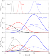 |
Fig. 5 Normalized radial profiles for the intrinsic |


Results for Ring0 models with different radii r0.
3.1.2 Radially extended scattering regions
Axisymmetric, radially extended disks or shells models are just superpositions of concentric ring signals, and the polarimetric cancellation effects will be strong for the innermost regions and much reduced further out. Therefore, the convolved polarization signal strongly underestimates the scattering near the central star and can mimic the presence of a central cavity even if no such cavity is present. The effect is illustrated in Fig. 6 with PSFAO convolved Qϕ(x, y) maps for the models Disk0α0, Disk0α−1, and Disk0α−2, with radial brightness profiles  , and Aϕ(r/rref)−2, respectively. In all three cases the intrinsic disk extends from rin = 3.15 mas or 0.125 DPSF to rout = 100.8 mas. The radius of the convolution hole (rh(Qϕ)) is slightly smaller than 0.4 DPSF for the α = −2 case and slightly larger than 0.4 DPSF for the α = −1 disk with a flatter brightness distribution (Table C.1).
Constant surface brightness. The convolution effects for Disk0α0 are shown in Fig. 7 with radial profiles for the intrinsic parameters  ,
,  and the convolved intensity Id(r) and polarization Qϕ(r) for different inner disk radii rin and for PSFG and PSFAO convolution. The profiles Id(r) show for increasing cavity size rin an increasing central dip depth and width. The surface brightness Id(r) is strongly reduced after convolution with PSFAO while the central cavity is less pronounced. The convolution does not change ΣId but for PSFAO a lot of the signal is redistributed to radii r ≫ 100 mas.
The convolved Qϕ(r) profiles show for all cases a central zero Qϕ(0) = 0, even for the disk without central cavity. Only models with rin ≈ DPSF or larger show an obvious difference when compared to the model without cavity. The Qϕ(r) profiles do not reach the intrinsic  level even for the convolution with a narrow PSFG, because of the polarimetric cancellation. For the convolution with PSFAO there is an additional reduction of the Qϕ(r) level by about 40% but despite this, the radial shape of the profiles is very similar for the two cases as follows also from hole radii rh(Qϕ) given in Table C.1.
Centrally bright scattering regions. Many circumstellar disks and shells show a steep surface brightness profile increasing strongly toward smaller radii. Therefore, the polarimetric cancellation suppresses efficiently the intrinsically very bright but barely resolved central signal (e.g., Avenhaus et al. 2018; Garufi et al. 2020; Khouri et al. 2020; Andrych et al. 2023).
Simulations of radial profiles are shown in Fig. 8 for PSFAO convolved models DiskI60α−2 with intrinsic surface brightness profile for the polarization  with rref = 12.6 mas and Aϕ = 20.7 similar to Eq. (5) and for different cavity sizes rin. The convolved profiles Qϕ(r) show clearly how the central hole size decreases for smaller rin, and how the measurable peak polarization signal max(Qϕ(r)) increases. Despite the strongly increasing intrinsic
  signal at small radii the convolved Qϕ(r) curves converge to a limiting model case with ri ≈ 0.2 DPSF (≈5 mas), because even large amounts of intrinsic signal in the center are fully cancelled by the convolution (Table C.1). The Qϕ(r) profiles are still quite sensitive for constraining the intrinsic
  signal around r ≈ DPSF based on the location of the flux maximum r(max(Qϕ)) and the amount of Qϕ(r) signal near this location. A careful analysis of Qϕ(r) can therefore constrain an inner cavity for a dust scattering region and this could be potentially useful for estimates on the dust sublimation radius for disks around young stars or the dust condensation radius for circumstellar shells around mass losing stars.
Details of the profiles Qϕ(r) depend also on the power law index α for the surface brightness. The peak radii r(max(Qϕ(r)) and central hole radii rh for a given rin are a bit larger for Disk0α−1 than Disk0α−2 (Table C.1), because in this model the contributions of smeared signal from larger separations are more important than for Disk0α−2 and this reduces the apparent sharpness of the central cancellation hole.
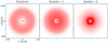 |
Fig. 6 Central cancellation holes in the Qϕ(x, y) maps for the models Disk0α0, Disk0α−1, and Disk0α−2 after convolution with the extended PSFAO. The size of the inner cavity rin = 0.125DPSF (3.15 mas) is the same for all three models and indicated by the black dot. |
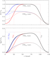 |
Fig. 7 Normalized profiles |


 |
Fig. 8 Radial profiles Qϕ(r) for the Disk0α−2 model convolved with PSFAO on a log-scale (upper panel) and a linear scale (lower panel) for different inner cavities r0 as indicated by the colors. The thin black line is the intrinsic surface brightness |

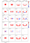 |
Fig. 9 Maps for the intensity Id and polarization Qϕ, Q, U, Qϕ, Uϕ, and P (from top to bottom) for RingI60 models with r0 = 12.6 mas, 25.2 mas, and 50.4 mas after convolution with the Gaussian PSFG (first three columns). The last column gives the same for the intrinsic model with r0 = 50.4 mas. Stokes quadrant parameters are indicated in some Q and U maps. |
3.2 Convolution for inclined disk ring models
The scattering geometry for a rotationally symmetric system with an inclined symmetry axis is not axisymmetric and then new features appear in the intensity and polarization maps. This is illustrated in Fig. 9 by the PSFG convolved maps for the scattered intensity Id and the polarization parameters Q, U, Qϕ, Uϕ, and P for RingI60 models with an inclination of i = 60◦ and r0 = 12.5 mas, 25.2 mas and 50.4 mas and including the intrinsic maps for the last case. The central star is assumed to be unpolarized, or Q = Qd, U = Ud and P = Pd, and the stellar intensity is not included in the Id(x, y) intensity maps. All RingI60 models have the same intrinsic polarization  .
.
The ring front side is much brighter because of the adopted forward scattering parameter g = 0.6 for the dust and this is clearly visible for the I′(x, y) and I(x, y) maps for r0 = 50.4 mas. This changes for the less resolved systems into a front-side intensity arc for r0 = 25.2 mas or r0 = DPSF and a slightly elongated spot offset toward the front side for r0 = 12.6 mas (0.5 DPSF).
The inclined models show a left-right symmetry for the intensity Id(x, y) = Id(−x, y), for Stokes Q, the azimuthal polarization Qϕ, and the polarized flux P. The Stokes U-parameter has a left-right antisymmetry Ud(x, y) = −Ud(−x, y), as well as the Uϕ-signal introduced by convolution effects.
The intrinsic Stokes parameters Q′(x, y) and U′(x, y) show positive and negative regions which can be characterized by the quadrant polarization parameters  ,
,  ,
,  , and
, and  for Stokes Q′ and
  ,
,  ,
,  , and
, and  for Stokes U′ as indicated in Fig. 9. They are useful for the characterization of the azimuthal distribution of the polarization based on the natural Stokes patterns produced by circumstellar scattering (Schmid 2021). Quadrant parameters have been calculated for simple models of debris disks (Schmid 2021) and of transition disks (Ma & Schmid 2022).
The intrinsic RingI60 models have strong positive Q090 and Q270 quadrants centered on the major axis of the projected disk, because of the high fractional polarization produced by scatterings with θ ≈ 90◦. The front side quadrant Q180 shows for well resolved systems a clear negative component, which is, however, less dominant than in intensity, because the fractional polarization of forward scattering is lower than for 90◦ scattering.
The negative Q000 and Q180 components disappear for not well resolved disks because the PSF smearing of the two strong positive components Q090 and Q270 cancel the signal of the negative Stokes Q quadrants. For the convolved RingI60 model with r0 = 12.6 mas there remain only two positive Qd-spots but their relative position still indicates the orientation of the projected major axis. The brighter disk front side produces in the Stokes Ud map a left side dominated by the positive U135 signal and a right side by the negative U225 component. This feature is still visible for barely resolved disks and this indicates the location of the disk front-side.
The intrinsic disk polarization of our models is azimuthal everywhere, and therefore the map  is equal P′(x, y), while
  , according to Eq. (10). The convolved maps Qϕ(x, y) for r0 = 50.4 mas represents well the intrinsic map appart from the smearing, but for less well resolved disks Qϕ(x, y) starts to display negative values above and below the center and for r0 = 12.6 mas a strong, central quadrant pattern for Qϕ(x, y) is visible as expected for an unresolved, central source with a positive Stokes ΣQ signal and ΣU = 0.
The convolution of the non-axisymmetric scattering polarization produces a Uϕ signal and we call this effect the convolution cross talks for the azimuthal polarization2 Qϕ → Uϕ. This effect increases with decreasing spatial resolution, and therefore the Uϕ(x, y) signal becomes stronger for less well resolved disks. For an unresolved disk the quadrant patterns for the azimuthal polarization Qϕ(x, y) = −Q(x, y) cos(2ϕxy) and Uϕ(x, y) = Q(x, y) sin(2ϕxy) are equally strong but rotated by 45◦. For the polarized flux P the convolved signal for large rings is roughly equal to the azimuthal polarization P(x, y) ≈ Qϕ(x, y), and for barely resolved rings it evolves toward P(x, y) ≈ Q(x, y) (Fig. 9).
3.2.1 Convolution and integrated polarization parameters
The convolution with a normalized PSF does not change the integrated Stokes polarization or the integrated intensity. Thus, there is for the RingI60 models ΣQ = ΣQ′ = 0.421  and ΣU = ΣU′ = 0, independent of the disk size or the spatial resolution. Contrary to this, the integrated polarization parameters ΣQϕ, ΣUϕ, and ΣP and the sums of absolute values Σ|Q| and Σ|U|, Σ|Qϕ| and Σ|Uϕ| depend on the resolution and the PSF convolution. The dependencies are plotted for the RingI60 models as a function of ring radius r0 convolved with PSFG and PSFAO in Fig. 10, and Table D.1 lists numerical values.
The red curves in Fig. 10 show ΣQϕ, which is large for well resolved disks and approaches zero for small, unresolved disks r0 → 0 when the Qϕ map shows a perfect positive-negative quadrant pattern with no net ΣQϕ polarization. For the intrinsic disk there is  and
and  and these relations are still approximately valid for well resolved disks convolved with PSFG because the convolution effects are small (Fig. 10a). The convolution with PSFAO introduces even for very extended disks strong smearing, because of the extended PSF halo (Fig. 10b). Therefore, ΣP is for well resolved disks larger than ΣQϕ by about 5% for the model with r0 ≈ 800 mas and about 18% for r0 = 201.6 mas (Table D.1).
For an unresolved scattering region r0 ≪ DPSF there remains only an unresolved polarized source with ΣP. Because of the alignment of the RingI60 models with the (x, y) disk coordinates, there is ΣQ = Σ|Q| = ΣP and ΣU = Σ|U| = 0. The azimuthal polarization is then zero ΣQϕ ≈ 0 and the integrated absolute values for the azimuthal polarization are Σ|Qϕ| = Σ|Uϕ| = (2/π) |ΣP| for the quadrant pattern of an unresolved source (Schmid 2021).
In the models a net signal in azimuthal polarization ΣQϕ > 0 or an integrated absolute signal Σ|Qϕ| larger than Σ|Uϕ| indicates the presence of at least a marginally resolved circumstellar polarization signal (Fig. 10). In observational data, ΣQϕ signals can also be produced by noise effects and one needs to derive for a given dataset the limits for a significant detection of a resolved circumstellar ΣQϕ-signal. However, one can expect for random noise sources introduced for example by the atmospheric turbulence, photon and read-out noise, that they produce also random positive and negative Qϕ and Uϕ signals, and different systematic effects like polarization offsets (see Sect. 4) or alignment errors produce no or only small positive or negative ΣQϕ and ΣUϕ signals. Therefore, the two criteria ΣQϕ > 0 and Σ|Qϕ| > Σ|Uϕ| are reliable indicators for the presence of resolved circumstellar polarization. Contrary to this, the ΣP signal is systematically enhanced by random noise and also polarization offsets change typically ΣP substantially.
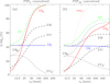 |
Fig. 10 Integrated polarization parameters for the RingI60 model as a function of the ring radius r0 after convolution with PSFG (a) and PSFAO (b). All parameters have been normalized to the intrinsic value |

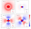 |
Fig. 11 Large-scale halo signals for the Stokes parameters Q, U and the azimuthal polarization Qϕ(x, y), Uϕ(x, y) for the RingI60 model with r0 = 50.4 mas convolved with PSFAO. The inset on the lower-right in each panel shows the disk ring in the center with a color scale reduced by 500 times. |
3.2.2 Halo signals produced by an extended PSFAO
The extended halo in the PSFAO of an adaptive optics system smears substantially the net Stokes polarization ΣQ, ΣU of a system over a large area producing an extended P(x, y) halo of linear polarization for r ≫ r0. This halo effect is illustrated in Fig. 11 for the PSFAO convolved RingI60 model with r0 = 50.4 mas, where the smeared ΣQ signal produces a polarized speckle ring ghost around r ≈ 0.4″ and a halo. The Stokes U signal in the halo is much weaker because there is no net U-signal for this model, and only a much weaker artifact pattern of the kind described in Appendix B is visible. The Q-halo produces extended Qϕ(x, y), Uϕ(x, y) quadrant patterns including the relatively strong speckle ring around r ≈ 0.4″, which shows the small scale imprint of the polarization from the bright ring.
The surface brightness of the halo is low and it can be difficult to recognize it in real data because of observational noise. Nonetheless, for the RingI60 model shown in Fig. 11 the Q-halo integrated in an annulus from r = 0.2″to 1.5″ is almost 30% of the system integrated ΣQ-signal (Table D.1). Therefore, it is important to use large integration apertures for the determination of ΣQ and ΣU for data convolved by an extended PSF.
The Qϕ signal in the halo integrated from r = 0.2″ to 1.5″ contributes less than 0.2% to the total ΣQϕ (Table D.1), because this signal has a positive-negative Qϕ, Uϕ quadrant patterns with zero net signal. Therefore, the measurement of ΣQϕ for a compact circumstellar scattering region should be restricted to a circular aperture which excludes the outer halo regions containing no net Qϕ signal but possibly substantial observational noise.
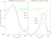 |
Fig. 12 Azimuthally averaged profiles for Qϕ(r), |Qϕ(r)|, and |Uϕ(r)| for the RingI60 models with r0 = 25.2 mas and 201.6 mas convolved with PSFAO. The green curve for the ratio |Uϕ(r)|/|Qϕ(r)| provides a rough measure for the convolution cross talk, and the dashed line indicates the system integrated value Σ|Uϕ|/Σ|Qϕ| from Table D.1. |
3.2.3 Convolution cross talk Qϕ → Uϕ or intrinsic Uϕ signal
The models considered in this work use a simpified description of the dust scattering which does no produce an intrinsic  polarization. However, it was pointed out in Canovas et al. (2015) that multiple-scattering by dust in optically thick protoplanetary disks with a non-axisymmetric scattering geometry can produce intrinsic
  signals representing non-azimuthal polarization components. Their simulations give
  signals of up to about ±5% of the azimuthal polarization
  and this U′-polarization can be useful to constrain the dust scattering properties and the disk geometry. This effect was also recognized in the disk models presented by Ma & Schmid (2022, Fig. 6).
As previously discussed, the PSF convolution can also produce very substantial Uϕ(x, y) signals for models with zero intrinsic  . This fact was already mentioned by Canovas et al. (2015), but they did not quantify this effect and their modeling used only a Gaussian PSF for the convolution.
The RingI60 simulations can be used to quantify the Qϕ → Uϕ convolution signal for different disk sizes r0. As a simple metric for this effect, we used the ratio Σ|Uϕ|/Σ|Qϕ| given in Table D.1 (see also the Σ|Uϕ| and Σ|Qϕ| curves in Fig. 10). For an unresolved disk, the convolution gives as an extreme limit a ratio of Σ|Uϕ|/Σ|Qϕ| = 1. The ratio is 0.22 and still high for the PSFG convolved disk with r0 = 50.4 mas plotted in Fig. 9. A larger disk of about r0 = 201.6 mas is requird to reach a low ratio of 0.03 so that an intrinsic Uϕ-signal could be detectable.
The situation is worse for disk models convolved with PSFAO producing substantially more Qϕ → Uϕ cross talk, and the ratio Σ|Uϕ|/Σ|Qϕ| is 0.19 for r0 = 201.6 mas and still larger than 0.1 for r0 = 806.4 mas The strong smearing of the Stokes Q-signal produces in the halo a ratio Σ|Uϕ|/Σ|Qϕ| ≈ 1. For a more detailed analysis the radial dependence of the ratio |Uϕ(r)|/|Qϕ(r)| should be considered, and such profiles are shown in Fig. 12 for PSFAO convolved RingI60 models with r0 = 25.2 mas and 201.6 mas. For the compact disk the |Qϕ(r)| signal is only at the separation of the ring r ≈ 12−35 mas substantially larger than |Uϕ(r)|, but nowhere more than a factor of 2. For the unresolved polarization near the center and for the smeared halo signal the ratio is |Uϕ(r)|/|Qϕ(r)| ≈ 1. For the larger disk, the Qϕ(r) signal dominates the Uϕ(r) cross talk signal by about a factor of 20 at the location of the inclined ring r ≈ 100−200 mas.
This indicates that an intrinsic  polarization at the level of 0.05
  is only detectable for large disks r0 ≳ 200 mas in high quality data for currently available AO systems, otherwise the convolution cross talks dominate. Helpful is, that the expected geometric structure of the observable Uϕ(x, y) signal produced by multiple scattering (see Canovas et al. 2015; Ma & Schmid 2022) is different from the Qϕ → Uϕ convolution artifacts, which can even be constrained strongly from the observed Qϕ(x, y) signal. In any case, the detection of the presence of intrinsic
  polarization requires high quality data of an extended scattering region and a very careful assessment of the convolution cross talk effects.
Uϕ signal and Qϕ uncertainty. In many studies the Uϕ signal is used as a proxy for the observational uncertainty for the measured Qϕ signal. This is a reasonable approach for cases with small Qϕ → Uϕ cross talk, like axisymmetric or close to axisymmetric scattering geometries, and very extended systems like RingI60 models with r ≳ 200 mas. The spurious signals introduces by speckle noise, read-out and photon noise, and small-scale instrumental artifacts in the Uϕ map are then larger than the convolution cross talk and therefore also representative for observational uncertainties in the Qϕ map.
However, for non-axisymmetric compact scattering regions the Uϕ signal consist mainly of the well-defined systematic convolution cross talk signal with high ratios |Uϕ(r)|/|Qϕ(r)| ≳ 0.5 like the RingI60 r0 = 25.2 mas model in Fig. 12. Despite this the azimuthal polarization signal Qϕ can still be highly significant, because for high quality data the observational noise in Qϕ is much smaller than the systematic Qϕ → Uϕ cross talk. In such cases another metric than the Uϕ signal must be used for the assessment of the observational uncertainties, like the dispersion of the measured results for different datasets or a detailed analysis of speckle and pixel to pixel noise in the data.
Nonetheless, a low |Uϕ| signal can be used to identify high quality data within a series of measurements taken under variable observing conditions. Because the systematic cross talk Qϕ → Uϕ is anti-correlated with the quality of the observational PSF one can select the polarization cycles with low |Uϕ| and this may provide a higher quality Qϕ map for a target.
3.2.4 Convolution and quadrant polarization parameters
The convolution can change for not well resolved RingI60 models strongly the azimuthal distribution of the polarization signal Qϕ(ϕ) and Uϕ(ϕ). This can be quantified with the quadrant polarization parameters which provide a simple formalism for the description of polarimetric convolution effects. We use the symbol Xxxx for all quadrant parameters, and Qxxx or Uxxx for the four Stokes Q or Stokes U quadrants, respectively. The quadrant values are related to the integrated Stokes parameters according to
 (13)
(13)
 (14)
(14)
For the mirror-symmetric RingI60 models, there is also ΣQ000 = ΣQ270, ΣU045 = −ΣU315, and ΣU135 = −ΣU225 (Schmid 2021).
The convolution changes the flux in the different Stokes quadrants because of smearing and mutual cancellation as can be seen in Fig. 9. This degradation is also illustrated for the normalized quandrant parameters  for the PSFG and PSFAO convolved RingI60 models as a function of r0 in the upper panels of Fig. 13 (see also Table D.1). For smaller and less resolved disks all Q-quadrants approach the same value ΣQxxx = ΣQd/4 as expected for an unresolved system with an integrated polarization ΣQd. For the Stokes U quadrants the effects are equivalent on both sides of the y-axis, and strong smearing turns the sign of the weaker back-side quadrants values U045 and U135 to the sign of the strong front side quadrants. This produces for compact disks positive signals for U045 and U135 “on the left side” of the star, and negative signals for U225 and U315 “on the right” side in Fig. 9 for the RingI60 model with r0 = 12.6 mas.
Differential quadrant parameters. Despite the smearing and polarimetric cancellation the information about the relative intrinsic strengths of the quadrant parameters can still be recovered to some degree as long as the scattering region is partially resolved. This is possible, because the mutual compensation of the polarization signal changes opposite sign quadrants roughly by similar amounts (Fig. 13 upper panel), and in step with the degradation of the total azimuthal polarization ΣQϕ shown in Fig. 10 for the same models.
Therefore, good values to constrain the intrinsic  fluxes are the relative differential values
 (15)
which quantify how much the individual Stokes Q quadrants contribute to the total Stokes Q signal (Eq. (13)) or how much more or less than the average contribution Q/4. According to Fig. 13 (lower left and Table D.2), the ∆Qxxx/ΣQϕ values are quite independent of the resolution for disks with r0 ≥ 50 mas, and one can still recognize for a RingI60 model disk with r0 ≈ 25 mas that the front side deviates more from the average than the back side. The relative differential quadrant values (Eq. (15)) are also practically the same for a convolution with PSFG and PSFAO and in very good agreement with the intrinsic values
(15)
which quantify how much the individual Stokes Q quadrants contribute to the total Stokes Q signal (Eq. (13)) or how much more or less than the average contribution Q/4. According to Fig. 13 (lower left and Table D.2), the ∆Qxxx/ΣQϕ values are quite independent of the resolution for disks with r0 ≥ 50 mas, and one can still recognize for a RingI60 model disk with r0 ≈ 25 mas that the front side deviates more from the average than the back side. The relative differential quadrant values (Eq. (15)) are also practically the same for a convolution with PSFG and PSFAO and in very good agreement with the intrinsic values
 (16)
(16)
The equivalent quantities for the Stokes U quadrants are just ratios (ΣUxxx/ΣQϕ) because the average value (ΣU/4) is zero. Figure 13 (lower right) shows, that the relative Stokes U quadrant ratios deviate for small disks with r0 ≲ 25 mas substantially from a constant. This is caused by the morphology of the Stokes U map for the RingI60 model, which has one dominant positive U135 and one dominant negative U225 quadrant. Smearing and cancellation affect the weak quadrants ΣU045 and ΣU315 stronger than the reference value ΣQϕ, while the effects between the strong components U135 and U225 are smaller than for ΣQϕ, because the separation between the strong components is relatively large.
A useful alternative are the relative differential values between the U quadrants on the positive or negative x-axis side:
 (17)
(17)
There is ∆U+ = −∆U− because of the symmetry of the RingI60 models. The ratio ∆U+/ΣQϕ is almost independent of the disk size r0 and the used PSF, according to the red line and points in Fig. 13 (lower right) and the values in Table D.2, which are very similar to the parameters ∆Qxxx/ΣQϕ. This demonstrates that differential quadrant parameters are useful to push the characterization of Qϕ(ϕ) and Uϕ(ϕ) for circumstellar scattering regions toward smaller separations.
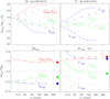 |
Fig. 13 Quadrant polarization parameters ΣXxxx normalized to the intrinsic azimuthal polarization |

3.3 Convolution of inclined extended disks
Extended disks with unresolved or partially unresolved central regions are frequently observed (e.g., Garufi et al. 2022) and it is of interest to investigate regions close to the star r < DPSF because they correspond to the zone of terrestrial planet formation ≲ 3 AU for systems in nearby star forming regions. In particular, the polarization of the unresolved part of the disk at r ≲ 0.5 DPSF (<12.6 mas) can be compared with the polarization of the resolved region r ≳ DPSF to constrain the presence or absence of significant changes in the scattering properties between the two regions.
Polarization maps for the inclined and extended DiskI60α-2 models are plotted in Fig. 14 with radii for the inner cavities of rin = 0.125 DPSF, 0.5 DPSF, and DPSF, or 3.15 mas, 12.6 mas, and 25.2 mas, respectively. The inner disk rim is very bright for these models, and therefore the convolved disk maps look similar to the images in Fig. 9 for small disk rings. The model with rin = DPSF in Fig. 14 shows a resolved Qϕ disk image with small cross talk residuals in Uϕ, while the disk with a very small cavitiy of rin = 0.125 DPSF has strong quadrant patterns for Qϕ and Uϕ as expected from the net Q-signal of a bright, unresolved central disk region.
The integrated polarization parameters for the DiskI60α−2 models depend strongly on the inner disk radius rin according to Fig. 15 or the numerical values given in Table D.3. The parameters are all normalized to the intrinsic azimuthal polarization  for the disk with rin = 0.5 DPSF. The intrinsic polarization parameters
  and ΣQ = ΣQ′ = 0.421
  are much larger for disks with small inner radii, for example by a factor 1.7 for rin = 0.125 DPSF when compared to rin = 0.5 DPSF. The convolution does not change the integrated Stokes polarization ΣQ = ΣQ′ but only redistributes spatially the signal Q′(x, y) → Q(x, y), and therefore the ΣQ curves are identical in the two panels of Fig. 15 for the models convolved with PSFG and PSFAO.
Contrary to this, the PSF convolution reduces or even cancels the strong  -signal of the central region and the effect is more important for PSFAO than for PSFG. Therefore, ΣQϕ reaches for a given convolution PSF a limiting value for models with a cavity smaller than rin < 0.5 DPSF, despite the fact that the intrinsic
  and ΣQ′ increase steeply for rin → 0 for the DiskI60α−2 model.
The central quadrant patterns in the convolved Qϕ and Uϕ maps have a strength proportional to the net Q signal from the unresolved inner disk region. The central Stokes signal ΣQc ≈ ΣQ(r ≲ 0.5 DPSF) and ΣUc can be used to constrain the amount of polarization Pc and the averaged polarization position angle (θc = 0.5 · arctan2(ΣUc, ΣQc)) for the unresolved part. Differences between θc and the averaged polarization position angle of the resolved signal θd for ΣQ(r≳ 0.5 DPSF) can point to a structural change between the unresolved and the resolved part of the scattering region, or to a contribution from interstellar or instrumental polarization as discussed in the next section.
The intrinsic profile  for the DiskI60α−2 models is steep, and therefore the ratio of convolved parameters ΣQ/ΣQϕ changes strongly with the radius of the inner cavity rin (Fig. 10). According to Table D.3 the dependence is smaller for the DiskI60α0 and DiskI60α−1 models. Nonetheless, ΣQ/ΣQϕ could be a good parameter to derive from observational data the radius rin of an unresolved central cavity or other disk properties at r < DPSF, in particular when using constraints about disk inclination and surface brightness profile from the resolved part of the disk at r ≳ DPSF.
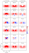 |
Fig. 14 Intrinsic maps |


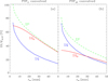 |
Fig. 15 Integrated polarization parameters ΣQϕ, ΣP, ΣQd for the inclined DiskI60α−2 model as a function of the radius of the inner cavity rin and for PSFG and PSFAO convolution. All values have been normalized to the intrinsic value |

3.4 The contribution of a polarized central star
The simulations presented up to now assume that the central star is unpolarized ( and
and  in Eqs. (3) and (4)), and therefore it does not affect the polarization signal of the circumstellar scattering region. However, often the stars with resolved circumstellar dust scattering regions have also unresolved components, as inferred for example from the thermal emission of hot dust. This dust can produce for the central, unresolved point-like source an intrinsic polarization, if scattering occurs in a non-symmetric structure. The central star can also be polarized by uncorrected contributions from interstellar or instrumental polarization. As the star is typically much brighter than the resolved circumstellar scattering already a small fractional polarization of the order ps = ΣQs/ΣIs ≈ 0.001 can have a strong impact on the observable polarization, and the following Sect. 4 addresses the question on how to correct for this.
In this subsection we explore the impact of a polarized central source on the imaging polarimetry of a circumstellar scattering region. For this, we have to distinguish between the stellar Qs, Us and circumstellar Qd, Ud polarization components. We consider a central point source with a fractional polarization  and position angle θs = 0.5 · atan2(us, qs) defined in disk coordinates (x, y). The convolved intensity distribution of the central source is Is(x, y) = ΣIs · PSF(x, y) and the corresponding Stokes parameter maps are Qs(x, y) = qs Is(x, y) and Us(x, y) = us Is(x, y). The integrated azimuthal polarization signals of the star are zero ΣQϕ,s = ΣUϕ,s = 0, but the corresponding convolved signal maps show the quadrant patterns
 (18)
(18)
 (19)
(19)
The strengths of these Qϕ,s and Uϕ,s quadrant patterns are independent of θs, but their orientation is defined by θs. The impact of the polarized intensity of the star ΣPs = ps ΣIs on the disk polarization map in convolved data depends of course on the relative strength between ΣPs and ΣQϕ,d.
Figure 16 shows as example a disk plus star system with an intrinsic ratio of of  for a system with disk intensity
  , disk polarization
  , and a stellar polarization of
  . The scattering region is simulated with the inclined disk model DiskI60α−2 with rin = 0.5 DPSF. The star polarization has an orientation θs = 67.5◦ (qs = −0.71ps, us = +0.71ps) and the whole system is convolved with PSFAO. This reduces the azimuthal polarization Qϕ,d of the disk and it results a ratio of ΣPs/ΣQϕ,d = 0.635 for the convolved model.
The polarization of the star has a strong impact on the polarization maps, despite the fact that ΣPs is weaker than the circumstellar polarization ΣQϕ,d. This is apparent in the maps in Fig. 16, in particular when compared to the disk maps of Fig. 14 without stellar polarization. The star produces in the center of the Stokes Q(x, y) map a strong negative signal, and in U(x, y) the antisymmetric appearance for the inner disk region is distorted. For the azimuthal polarization strong quadrant patterns for Qϕ(x, y) and Uϕ(x, y) are visible around the position of the central star.
The azimuthally averaged radial profiles for psIs(r) and Qϕ,d(r) in Fig. 17 show that the stellar polarization dominates strongly for r < 20 mas, where the stellar intensity Is(r) is much higher than the disk intensity Id(r), while the disk polarization is the main polarization component in the range r ≈ 30–120 mas.
There are three important properties for the interpretation of the polarization signal: (i) the integrated Stokes parameters do not depend on the PSF convolution, and therefore the disk and star signal are added together
 (20)
(20)
 (21)
(21)
(ii) ΣQϕ and ΣUϕ do not depend on the polarization signal of an unresolved central object because the introduced quadrant patterns add no net signal, i.e., ΣQϕ,s = 0 and ΣUϕ,s = 0; (iii) the orientation of the central Qϕ and Uϕ quadrant patterns are defined by θs of the central source.
If the polarization of the central source is aligned with the resolved disk θs = θd, then we expect a left right symmetry Qϕ(x, y) = Qϕ(−x, y) for the overall Stokes Qϕ map and an antisymmetry Uϕ(x, y) = −Uϕ(−x, y) for Stokes Uϕ like for the partially resolved disks shown in Fig. 14. Deviations from these properties are indicative for a more complicated polarization structure with a stellar polarization component not aligned with the disk polarization.
Interstellar and instrumental polarization. The impact of polarization offsets from interstellar pisI(x, y) or instrumental pinstI(x, y) polarization are proportional to the total intensity, while an offset from an intrinsically polarized star psIs(x, y) is proportional to the PSF of the star. However, for many typical cases one can approximate ps Is(x, y) ≈ ps I(x, y) because the difference between stellar and total intensity, which is equivalent to the scattered intensity from the dust Id(x, y), is very small for circumstellar scattering regions.
This is is supported by the azimuthal profiles in Fig. 17 for the disk plus star model described above (Fig. 16). In this example the disk polarization in the range r ≈ 30–120 mas is much larger than the difference between the polarization offsets of p = 0.001 for the total intensity and the stellar intensity Qϕ(r) ≫ (p(I(r) − Is(r)). Therefore it makes for this example practically no difference for the disk polarization signal Qϕ(x, y) whether one uses p I(x, y) or p Is(x, y) for the polarization offset correction.
This approximation is also valid for faint circumstellar scattering regions, if the fractional scattering polarization is at the same level ΣQϕ ≈ 0.1 ΣId as in the example shown above, because the difference for the two cases of polarization offsets scales still with ΣId according to p (I(r) − Is(r)) = p Id(r). The approximation I ≈ Is is less good for a bright scattering region Id, in particular if the polarization offsets is large p ≳ 0.01 and the scattering region weakly polarized ΣQϕ/ΣId ≲ 0.1, and combination of these cases.
We treat in this study an intrinsic stellar polarization like an interstellar polarization offset. Interstellar and instrumental polarization offsets can be corrected using pis I(x, y) or pinst I(x, y) with the advantage, that the system intensity I(x, y) can be derived from unsaturated observations of the target. In the best case I(x, y) is obtained simultaneously with the polarization signal Q(x, y) and U(x, y) so that atmospheric variations can be taken accurately into account (e.g., Tschudi & Schmid 2021). Using the system intensity I(x, y) also as approximation for the correction of an intrinsic stellar polarization ps I(x, y) ≈ ps Is(x, y) overestimates slightly the offset, but avoids the difficult procedure of splitting I(x, y) into a stellar PSF component Is(x, y) and a disk component Id(x, y). Using Is(x, y) instead of I(x, y) would provide in many cases only a marginal improvement for the offset correction when considering other PSF calibration issues in high contrast imaging polarimetry.
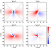 |
Fig. 16 Polarization maps Q, U, Qϕ, Uϕ for the model DiskI60α−2 (rin = 0.5 DPSF or 12.6 mas) and a polarized central star with |


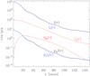 |
Fig. 17 Azimuthally averaged intensity profiles for the disk, Id(r); the star, Is(r); and the total, I(r), for the disk polarization, Qϕ(r), and the intrinsic stellar polarization, psIs(r), or interstellar polarization, pisI(r), introduced by a fractional offset of p = 0.1%. The same disk model, polarization offset psIs(r), and PSFAO convolution as in Fig. 16 is used, while the interstellar offset for pisI(r) is applied to the total intensity. |
4 Polarimetric calibration and zp-correction
4.1 The impact of a fractional polarization offset
Already a small fractional polarization offset of the order p ≈ 0.1% from an intrinsic polarization of the central star, from interstellar polarization, or from instrumental polarization can have a strong impact on the observed polarization maps of circumstellar scattering regions (Fig. 16). Unfortunately, the different polarization effects are often not well known, and after a calibration there can remain non-negligible polarization residuals, pres, with an arbitrary position angle, θres, or a residual fractional Stokes values, qres and ures:
 (22)
(22)
 (23)
(23)
This can also be expressed by the integrated parameters
 (24)
and equivalent for the Stokes U polarization component. The residual offset pres ΣI can strongly disturb or even dominate the weak polarization signal Qd, Ud of the circumstellar scattering region. The standard method to improve the situation is a polarimetric zp-correction, which cancels the integrated Stokes signals,
(24)
and equivalent for the Stokes U polarization component. The residual offset pres ΣI can strongly disturb or even dominate the weak polarization signal Qd, Ud of the circumstellar scattering region. The standard method to improve the situation is a polarimetric zp-correction, which cancels the integrated Stokes signals,
 (25)
(25)
 (26)
in a certain apperture, Σ, using the fractional Stokes parameters ⟨qobs⟩ = ΣQobs/ΣI and ⟨uobs⟩ = ΣUobs/ΣI (e.g., Quanz et al. 2011; Avenhaus et al. 2014). This is a powerful method to find the circumstellar polarization component in data dominated by residual interstellar, instrumental, or stellar polarization offsets.
(26)
in a certain apperture, Σ, using the fractional Stokes parameters ⟨qobs⟩ = ΣQobs/ΣI and ⟨uobs⟩ = ΣUobs/ΣI (e.g., Quanz et al. 2011; Avenhaus et al. 2014). This is a powerful method to find the circumstellar polarization component in data dominated by residual interstellar, instrumental, or stellar polarization offsets.
The zp-correction is also very useful for data, where a circumstellar polarization is detected, but where the signal might be affected by an unknown offset qres. Because ⟨qobs⟩ = ΣQ/ΣI + qres according to Eq. (24) and using Eq. (25) gives
 (27)
with ⟨q⟩ = ΣQ/ΣI and equivalent for ΣUz. This means, that the zp-corrected signals of a Stokes map with a fractional polarization offset, e.g. because of calibration uncertainties, is equal to the zp-corrected signal of the map without offsets like for perfectly calibrated data. Therefore, the zp-correction provides data with a well-defined offset correction, which can be re-calibrated later Qz(α, δ) → Q(α, δ) in a second step once the intrinsic offset value ⟨q⟩ is known from more accurate polarimetry or constraints from scattering models. For example, for a given object the same zp-corrected Stokes signals ΣQz, ΣUz should result for data affected by different instrumental polarization offsets pres. The Stokes maps Qz(α, δ), Uz(α, δ) still depend on the observational PSF.
(27)
with ⟨q⟩ = ΣQ/ΣI and equivalent for ΣUz. This means, that the zp-corrected signals of a Stokes map with a fractional polarization offset, e.g. because of calibration uncertainties, is equal to the zp-corrected signal of the map without offsets like for perfectly calibrated data. Therefore, the zp-correction provides data with a well-defined offset correction, which can be re-calibrated later Qz(α, δ) → Q(α, δ) in a second step once the intrinsic offset value ⟨q⟩ is known from more accurate polarimetry or constraints from scattering models. For example, for a given object the same zp-corrected Stokes signals ΣQz, ΣUz should result for data affected by different instrumental polarization offsets pres. The Stokes maps Qz(α, δ), Uz(α, δ) still depend on the observational PSF.
The zp-correction has practically no impact on the integrated azimuthal polarization ΣQϕ, and there is
 (28)
because a fractional Stokes polarization offset introduces for the Qϕ(α, δ) and Uϕ(α, δ) maps positive-negative quadrant patterns with a zero net signal. Therefore, ΣQϕ is a very robust quantity, which is hardly affected by polarization offsets introduced by calibration uncertainties. However, it is important to note that the zp-correction changes the signal distribution in the Stokes maps Qz(α, δ), and Uz(α, δ) and this can produce a strong bias for the measured azimuthal distribution of the
(28)
because a fractional Stokes polarization offset introduces for the Qϕ(α, δ) and Uϕ(α, δ) maps positive-negative quadrant patterns with a zero net signal. Therefore, ΣQϕ is a very robust quantity, which is hardly affected by polarization offsets introduced by calibration uncertainties. However, it is important to note that the zp-correction changes the signal distribution in the Stokes maps Qz(α, δ), and Uz(α, δ) and this can produce a strong bias for the measured azimuthal distribution of the  polarization which must be considered for the interpretation of zp-corrected data.
4.2 Cases without zp-correction bias
Polarimetric calibration uncertainties can be corrected with a zp-correction without introducing a bias, if the central source is intrinsically unpolarized ( ,
,  or ΣQd = ΣQ, ΣUd = ΣU) and can be used as zero polarization reference. The zp-correction value ⟨q1⟩ = Σ1Q/Σ1I derived for a small stellar aperture Σ1 then accounts for the polarization offsets, qres, introduced by the interstellar and instrumental polarization according to
 (29)
and equivalent for Stokes Uz1 component. This approximation assumes that the scattering region does not contribute to the polarization signal in Σ1.
(29)
and equivalent for Stokes Uz1 component. This approximation assumes that the scattering region does not contribute to the polarization signal in Σ1.
The central star cannot be used as calibration source for coronagraphic observations. However, if the object has an axisymmetric scattering geometry with zero or close to zero net polarization Σ2Q ≈ 0 and Σ2U ≈ 0, measured in an annular aperture Σ2, then this signal can be used as zero polarization reference. Good examples for such axisymmetric systems are circumstellar disks seen pole-on, like for TW Hya, HD 169142 or RX J1604 (Rapson et al. 2015; van Boekel et al. 2017; Poteet et al. 2018; Tschudi & Schmid 2021; Ma et al. 2023).
4.3 Bias introduced by the polarimetric zp-correction
The zp-correction is usually applied to the Q(α, δ) and the U(α, δ) frames in the sky coordinate system. We investigate the zp-correction effects in the (x, y) coordinate system of inclined disks, because the impact of polarization offsets does not depend on the orientation of the selected coordinate system. This simplifies the comparison of Qz(x, y), Uz(x, y) with the signal of the convolved models Q(x, y), U(x, y) representing perfectly calibrated data. The corrected signal depends on the selected correction region Σzp and different cases are considered including the zp-correction of coronagraphic data, or systems with partly unresolved disks.
4.3.1 ZP-correction for an inclined disk ring model
We considered the inclined model RingI60 with r0 = 100.8 mas in (x, y) coordinates convolved with the extended PSFAO, applied a zp-correction, and compared the corrected Stokes signal Qz(x, y) with the corresponding disk signal Q(x, y) without offsets. An overview on the used polarization parameters for zp-corrected models is given in Table A.2.
The zp-correction offset derived from a large aperture Σzp = Σ with a radius of r = 1.5″ yields for the corrected signal integrated in the same aperture ΣQz = ΣQ − ⟨q⟩ ΣI = 0 according to Eq. (27). This procedure compensates the positive disk polarization ΣQ by a negative offset −⟨q⟩ ΣI. The spatial distribution of the Stokes Q signal differs between the zp-corrected and the initial signals by
 (30)
(30)
For Stokes U there is Uz(x, y) = U(x, y) for the RingI60 models because ΣU = 0, and therefore ⟨u⟩ = 0. Thus, a Stokes Q zp-correction has no impact on the Stokes U signal and vice versa. Therefore the zp-correction effects described for Stokes Q can be generalized to an offset with Q and U components.
The zp-correction effects are illustrated in Fig. 18 with RingI60 maps of the polarization parameters X = {Q, U, Qϕ, Uϕ, P} for the convolved model X(x, y), the Σzp = Σ corrected model Xz(x, y), and the Σ2 corrected case Xz2(x, y) to be discussed later (Sect. 4.3.3). For Stokes Q a strong negative signal is introduced in the Qz(x, y) map at the position of the star, and because of the extended PSFAO, there are also negative contributions further out. Therefore, the corrected polarization Qz is also lower than Q at the location of the disk ring, while there is no difference between Uz(x, y) and U(x, y). The zp-corrected azimuthal polarizations  and
and  show the additional quadrant patterns for a convolved central point source with a negative Stokes Q polarization. For the polarized intensity P the offset −⟨q⟩ ΣI adds predominantly a positive component to the Pz(x, y) map.
The impact of the zp-correction in the Stokes polarization maps depends on the separation from the center, and therefore in addition to the total system integration region Σint = Σ, we can also consider three radial integration regions: Σ1, Σ2, and Σ3. These regions are indicated in Fig. 18 in the Qϕ(x, y) panel. They represent the star, the disk, and the halo regions, and they cover together the total system integration region Σ1 + Σ2 + Σ3 = Σ.
In the following a detailed description for the system-corrected map Qz(x, y) in Fig. 18 is given. The negative signal Σ1Qz in the stellar aperture Σ1 with r < 0.027″ introduced by the zp-correction can be estimated using Σ1Qz = Σ1Q − ⟨q⟩ Σ1I, which is Eq. (27) applied to the integration region Σ1. The disk contribution is very small Σ1Q ≈ 0 and the PSFAO convolved intensity Σ1I is about 40% of the total intensity ΣI (see Table E.1 for accurate values), and we obtained
 (31)
(31)
In the halo region Σ3 (0.2″ < r < 1.5″) there is roughly everywhere the same fractional polarization Q(x, y)/I(x, y) ≈ Σ3Q/Σ3I ≈ ⟨q⟩ for the convolved model, because far from the center the PSFAO smearing of the intrinsic Stokes signal Q′(x, y) of a compact disk is very similar to the smearing of the total intensity I′(x, y) dominated by the central star. Therefore, the halo signal is practically cancelled by the zp-correction and Eq. (27) for Σ3 can be approximated by
 (32)
(32)
Of importance for the analysis of the disk polarization is the annular aperture Σ2 with 0.027″ < r < 0.2″ covering the disk, and there is (using Eq. (27) for Σ2)
 (33)
(33)
Because ΣQz = 0 for the entire system r < 1.5″ and Σ3Qz ≈ 0 for the halo, the polarization for the zp-corrected disk region Σ2Qz is equal to the negative signal of the central star, or
 (34)
where the second relation is equal to Eq. (31). The Stokes Q polarization is after zp-correction Σ2Qz ≈ +0.44 ΣQ, which is significantly lower than for the non-corrected disk Σ2Q ≈ +0.71 ΣQ (Table E.1). Thus, the zp-correction introduces for the PSFAO convolved RingI60 model a strong bias for Stokes Q, changing also the angular distribution of the azimuthal polarization
(34)
where the second relation is equal to Eq. (31). The Stokes Q polarization is after zp-correction Σ2Qz ≈ +0.44 ΣQ, which is significantly lower than for the non-corrected disk Σ2Q ≈ +0.71 ΣQ (Table E.1). Thus, the zp-correction introduces for the PSFAO convolved RingI60 model a strong bias for Stokes Q, changing also the angular distribution of the azimuthal polarization  .
.
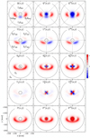 |
Fig. 18 Polarization maps for the RingI60 model with r0 = 100.8 mas convolved with PSFAO. The columns shows, from left to right, the convolved maps X(x, y), the maps Xz(x, y) for a system zp-correction, and Xz2(x, y) for disk zp-correction. The circles describe the integration regions Σ1, Σ2, and Σ3 as indicated in the Qϕ(x, y) panel and quadrant regions Σ2Xxxx are identified in the Q(x, y) and U(x, y) panels. |
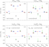 |
Fig. 19 Relative quadrant polarization parameters Σ2Xxxx (♢) and their azimuthal values Σ2Xxxx|ϕ (horizontal bars) for the disk integration region Σ2 for RingI60 with r0 = 100.8 mas: (a) instrinsic model, (b) convolved model, (c) Σ corrected model, and (d) Σ2 corrected model. The green and grey lines in (b) indicate the change of Σ2Xxxx and Σ2Xxxx|ϕ, respectively, with respect to panel a, and in the panels c and d with respect to panel b. All vallues are normalized to |

4.3.2 ZP-correction and quadrant polarization parameters
The intrinsic angular distribution of the azimuthal polarization  is changed in polarimetric observations, first by the instrumental convolution as described by the quadrant parameters ΣXxxx in Sect. 3.2.4, and, if applied, also by the polarimetric zp-correction. A Stokes Q zp-correction adds a signal −⟨q⟩ I(x, y), and because we adopted only axisymmetric PSFs and approximate I(x, y) ≈ Is(x, y), this introduces for all Stokes quadrants ΣintQxxx practically the same offset. These simple dependencies of the quadrant parameters is very useful to describe the convolution and zp-correction effects of the observed azimuthal polarization signal Qϕ(ϕ), which contains important information about the scattering geometry and the dust scattering properties.
The impact of the convolution and zp-correction are illustrated in Fig. 19 (upper panels) for the RingI60 (r0 = 100.8 mas) model with the quadrant polarization parameters Σ2Xxxx (diamonds) measured inside the integration region Σ2 extending from r = 27 mas to 200 mas as defined in Fig. 18 (panels Q(x, y) and U(x, y)). The quadrant values Xxxx represent different azimuthal parts ϕxxx of the polarizaton signal Qϕ(ϕ), but one needs also to consider whether the sign of Xxxx corresponds to a positive or negative contributions to the azimuthal polarization Qϕ. Therefore, we defined azimuthal quadrant values ΣiXxxx|ϕ, that account for the sign of the Stokes polarization with respect to Qϕ(ϕxxx) as follows:
For the Stokes Q quadrants, ΣiQ000|ϕ = −ΣiQ000, ΣiQ090|ϕ = +ΣiQ090, ΣiQ180|ϕ = −ΣiQ180, and ΣiQ270|ϕ = +ΣiQ270.
For the Stokes U quadrants, ΣiU045|ϕ = −ΣiU045, ΣiQ135|ϕ = +ΣiU135, ΣiU225|ϕ = −ΣiU225, and ΣiU315|ϕ = +ΣiU315.
The ΣiXxxx|ϕ values are plotted in Fig. 19 as horizontal bars. For the intrinsic disk model they are just equal to the absolute value of the quadrant values  , but this is not always the case for convolved and corrected models. From the change of the ΣiXxxx|ϕ values for the different cases one can estimate the change of the azimuthal distribution of Qϕ(ϕ) for angles ϕxxx representative for a particular quadrant.
The convolution changes the relative strengths of the quadrants as already described in Sect. 3.2.4 for the total system integration region Σ. In this section, we concentrate on the quadrant signals in the disk integration region Σ2 of the model RingI60 (r0 = 100.8 mas) and in Fig. 19 (panel b) the differences between the intrinsic and the convolved quadrant values Σ2Xxxx (diamonds) are illustrated by the vertical green lines and for the azimuthal quadrant values Σ2Xxxx|ϕ (bars) by grey lines. The mutual cancellation and the smearing of signal into the halo region Σ3 reduces the signal in Σ2 for the positive quadrants and enhances it for the negative quadrants and this corresponds to a substantial reduction of the absolute quadrant values |Σ2Xxxx| and of the corresponding azimuthal values Σ2Xxxx|ϕ in step with reduction for ΣQϕ (see also Table E.1).
The zp-correction compensates the disk polarization Σ2Q by adding a negative signal −Σ2Q with a distribution like I(x, y) and this reduces the polarization in Σ2 by ∆2Q = Σ2Qz − Σ2Q = −⟨q⟩ Σ2I according to Eq. (33). For the RingI60 model with r0 = 100.8 mas the effect is equal to  (Table E.1). All the Stokes Q quadrant values are changed by roughly the same amount,
 (35)
with
(35)
with  . The Stokes U quadrants are not changed, because Σ2U = 0 for the used model. Also the integrated azimuthal polarization Σ2Qϕ is practically not changed by the zp-correction offset.
Because of the correspondence between Qϕ(ϕ) for different ϕ-wedges and the azimuthal quadrant parameters, the negative Σ2Q/4 contribution is equivalent to a positive contribution for Σ2Q000|ϕ and Σ2Q180|ϕ, and a negative contribution for Σ2Q090|ϕ and Σ2Q270|ϕ as illustrated by the grey vertical lines in panel (c) of Fig. 19. This zp-correction enhances the relative signal of the disk front side by more than 50% or from  to
to  between the “non-corrected” and the zp-corrected disk maps (Table E.1). If one compares the ratio Σ2Q180|ϕ/Σ2Q090|ϕ between the signal on the front side with respect to the signal in the left or right quadrants, which are reduced by the zp-correction then the initial ratio is boosted from Σ2Q180|ϕ/Σ2Q090|ϕ = 0.32 to
  , or almost a factor of two. This example illustrates that the azimuthal distribution of the polarization signal Qϕ(ϕ) can be very significantly changed by a polarimetric zp-correction.
4.3.3 ZP-correction for coronagraphic observations
Annular appertures must be used for the zp-correction of coronagraphic observations or data with detector saturation at the position of the bright central star. Thus, one needs to consider other zp-correction regions than Σzp = Σ for the whole system. The resulting zp-corrected maps, integrated Stokes parameters, or quadrant parameters are identified with a superscript like Qz2, Qz3 or Qz2+3 for zp-corrections applied to the annuli Σzp = Σ2, Σ3 or Σ2+3 representing the disk region, the halo region, or the disk plus halo region, respectively. Table E.1 gives an overview on how the polarization parameters for different integration regions Σi depend on the used correction region Σzp for the model RingI60 with r0 = 100.8 mas. Important are the resulting polarization values for the annular aperture Σ2 which includes the disk ring.
The zp-correction applied to a given annulus Σzp = Σi sets the corrected Stokes value in this region ΣiQzi to zero according to ΣiQzi = ΣiQ − ⟨qzi⟩ ΣiI = 0, which is a generalization of Eq. (27). Selecting different zp-correction regions introduces different offsets ⟨qzi⟩ factors, and for the RingI60 models, the ⟨qzi⟩ values behave as follows:
 (36)
(36)
ZP-correction for the disk. The largest offset ⟨q2⟩ results for a zp-correction based on the disk region with a strong positive Σ2Q polarization. This sets Σ2Qz2 polarization to zero, or the positive quadrants ( ) equal to the negative quadrants
  and produces apparently a very strong
  signal for the disk front side as shown in panel d of Fig. 19 (Table E.1). This is only a zp-correction effect and should not be interpreted as real azimuthal distribution of the Qϕ(ϕ) signal, as would be expected for a disk with highly forward scattering dust.
Moreover, the derived correction offset ⟨q2⟩Σ2I = Σ2Q depends on the quality of the PSF. It is difficult to account for this, particularly for extended disks without sharp structures as in the RingI60 models. Thus, whenever possible one should avoid a zp-correction based on the disk region. This can be problematic for coronagraphic observation of faint disks with large outer radii r0, where the halo region r > r0 has not enough signal for a well-defined offset correction.
A zp-correction based on the whole region outside the coronagraphic mask Σzp = Σ2+3 reduces the correction offset (Table E.1). In the halo the smeared stellar intensity dilutes more efficiently the smeared disk Stokes signal, and there is ⟨q2+3⟩ < ⟨q2⟩. Thus, the zp-correction offset is reduced, but it depends still significantly on the PSF profile.
ZP-correction for the halo. For the halo there is ⟨q3⟩ ≈ ⟨q⟩ because the smearing of a ΣQ signal of a compact disk model like RingI60 with r0 = 100.8 mas is very similar to the smearing of the intensity, which is dominated by the star. Therefore the halo zp-corrected disk polarization is practically identical to the system zp-corrected signal (Table E.1), or
 (37)
(37)
The offset defined by the system zp-correction −⟨q⟩ΣI does not depend on the PSF profile, and this is also the case for the halo corrected models. This also applies, at least approximately, for coronagraphic observations and they should be corrected based on the halo region Σzp = Σ3 outside the disk because of the well-defined and relatively small bias offset.
For coronagraphic observations or data with detector saturation at the position of the star there is the fundamental issue that the PSF profile and the total intensity of the system ΣI cannot be derived from the same data. Flux and PSF calibrations are therefore required for quantitative measurements to allow for a correction of the convolution effects and to relate the measured polarization signal to the intensity of the central star, which is typically a good flux reference.
Coronagraphic observations of a large ring. A RingI60 model with r0 = 403.2 mas convolved with PSFAO provides a good example for the effects of a zp-correction for coronagraphic observations of an extended disk taken with a currently available instrument. Figure 20 shows the Stokes Q(x, y) map, and the zp-corrected maps Qz3(x, y), Qz2+3(x, y), and Qz2(x, y) while corresponding numerical values are given in Table E.2. The Σ1 region with the central star is defined by r < 100 mas and assumed to be covered by a coronagraphic mask. The region Σ2 with the circumstellar disk is described by the annulus 0.1″ < r < 0.5″ and Σ3 for the halo by 0.5″ < r < 1.5″. A very narrow color scale was selected to illustrate the weak extended signal.
The intrinsic disk has a positive net signal ΣQ and this produces in the convolved map Q(x, y) an extended halo with a faint, positive Q signal (Fig. 20a). A zp-correction applied to the coronagraphic data Σzp = Σ2+3 cancels the net positive polarization in the Σ2+3 region and this turns the positive background in Q(x, y) into a negative background in the corrected map for Qz2+3 (Fig. 20c). Moreover, the subtraction −⟨q2+3⟩ I(x, y) produces a quite significant ring of negative Q polarization at the position of the PSF speckle ring typical for AO systems. This correction artifact can disturb significantly the analysis despite the fact that the disk signal is very well resolved. The bias effects is smaller, if the halo region is used for the zp-correction Σzp = Σ3 and larger, if only the disk region is used Σzp = Σ2 (see Figs. 20b,d or Table E.2).
Determining the zp-offset ⟨q3⟩ from the halo is therefore also for coronagraphic observations of extended disks, like the example in Fig. 20, a good approach for a well-defined ⟨q3⟩ ≈ ⟨q⟩ zero point correction. For this, one should select a region which represents well the average fractional polarization of the system, like the region outside the AO speckle ring. This feature should be avoided, because it overrepresents the stellar contribution.
Speckle ring as stellar polarization signal. The AO speckle ring in high contrast coronagraphic data can be strong and could be used to measure or estimate the polarization of the star ΣQs/ΣIs and ΣUs/ΣIs. The requirement is, that stellar light in the speckle ring can be separated well from the circumstellar scattering signal.
This could be the case for a small scattering region located clearly between coronagraphic mask and the stellar speckle ring in particular if the disk polarization has a small net Stokes Q and U signal so that the smeared halo of the disk is almost unpolarized. The polarization of the stellar speckle ring can probably also be measured quite well for a circumstellar regions similar to the coronagraphic model in Fig. 20 because the speckle halo at ∆y ± 450 mas above and below the star is well separated from the disk signal.
The derived fractional polarization from the stellar speckles can then be used as approximation for ΣQs/ΣIs and ΣUs/ΣIs and be used for a polarimetric zp-correction. If the star is unpolarized, then one would get well calibrated coronagraphic polarization data Q(x, y) and U(x, y) like for the case described in Sect. 4.2. Applying specific procedures for a given dataset must probably be considered to achieve the best results, but this is beyond the scope of this paper.
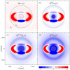 |
Fig. 20 Effects of the zp-correction for Stokes Q for the PSFAO convolved RingI60 model with r0 = 403.2 mas for observations with a coronagraphic mask, indicated by the central hatched area. Panel a shows the convolved signal Q(x, y), b shows the map after a correction based on the halo Qz3, c shows the map after correction based on the disk plus halo Qz2+3, and d shows the map after correction based on the disk region Qz2. The peak Q signal is in all panels between 22 and 23 units with respect to the indicated color scale. |
4.4 Partially resolved circumstellar scattering regions
Many circumstellar disks and shells are too small to be fully separated from the star. The PSFAO convolved DiskI60α−2 model with a small inner cavity rin = 3.15 mas represents such a situation. The circumstellar scattering in this model produces a substantial amount of unresolved Stokes Qd signal in the center (Fig. 21, left panels). The zp-correction for the system (middle panels) sets the integrated ΣQz signal to zero and therefore produces a strong −Q signal in the center and correspondingly strong central quadrant patterns for the Qϕ and Uϕ map with opposite sign when compared to the convolved model. In both cases the strong central Q signal disturbs substantially the relatively faint signal of the spatially resolved part of the disk, and it is difficult to separate the two polarization components.
4.4.1 ZP-correction for the center
The polarization offset introduced by the central source can be removed with a star peak or center zp-correction where the offsets, ⟨q0⟩ = Σ0Q/Σ0I and ⟨u0⟩ = Σ0Q/Σ0I, are derived from a few pixels centered on the intensity peak. This sets the Stokes Q polarization signal at the center to zero,
 (38)
and equivalent for the Stokes U component Uz0(0, 0). In Fig. 21 it removes the strong central Stokes Q-component and quadrant patterns in the Qϕ and Uϕ maps. The center correction leaves an extended polarization signal from circumstellar scattering, called hereafter Qex, Uex, according to
(38)
and equivalent for the Stokes U component Uz0(0, 0). In Fig. 21 it removes the strong central Stokes Q-component and quadrant patterns in the Qϕ and Uϕ maps. The center correction leaves an extended polarization signal from circumstellar scattering, called hereafter Qex, Uex, according to
 (39)
(39)
 (40)
(40)
The polarization in the PSF peak ⟨q0⟩ I(0, 0) and ⟨u0⟩ I(0, 0) can include contributions from the following components: (i) offsets introduced by (residual) interstellar and instrumental polarization, (qis + qinst) I, (uis + uinst) I, and (ii) the intrinsic central polarization, Qc = qsIs + qd,cIs and Uc = usIs + ud,cIs, from the star and the unresolved part of the scattering region.
The offset from the center correction is proportional to I(α, δ) and therefore it corrects accurately the signal introduced by the interstellar and instrumental polarization. In addition also the contribution from the intrinsic stellar polarization Qc, Uc are corrected, but only approximately because the intensity distribution of the convolved central signal is ∝PSF(α, δ) and differs slightly from I(α, δ) used for the correction offset. This introduces a small overcorrection at the level of (qs + qd,c) Iext(α, δ)/Is(α, δ) and similar for Stokes U, where Iext corresponds to the resolved part of the scattering intensity. There is typically (qs + qd,c)Iext(r) ≪ Qϕ(r) based on simular arguments as discussed in Sect. 3.4, and therefore we can assume that the center correction accounts for many cases well for all contributions to the polarization of the central source.
The center-corrected maps Xex(x, y) for the DiskI60α−2 model with small cavity rin = 0.125 DPSF in Fig. 21 look very similar to the non-corrected DiskI60α−2 model with a larger inner cavity with r0 = 0.5 DPSF plotted in Fig. 14. Thus, the effect of the center zp-correction is very similar to the removal of the polarization signal from the non-resolved inner disk region r < 0.5 DPSF (Table E.3).
The zp-correction for the center splits the integrated polarization into a central unresolved component and an extended resolved component:
 (41)
(41)
For simulations with a given intrinsic model but using different PSFs for the convolution the total Stokes signals, ΣQ and ΣU are conserved, but the splitting between the ΣQ0 and ΣQex or the ΣU0 and ΣUex components depends on the PSF profile. For a more extended PSF a larger fraction of the polarization signal will contribute to the unresolved central source and a smaller fraction to the extended (resolved) component.
The impact of the center correction for the ΣQ splitting is illustrated in the left panel of Fig. 22 for DiskI60α−2 models with different rin. For large central cavities rin > DPSF (>25 mas) there is practically no difference between ΣQex and ΣQ because of the lack of a central component. For small cavitity rin < DPSF the unresolved central signal ΣQ0 ≈ ⟨q0⟩ ΣI plotted by the green curve increases strongly for rin → 0, while the extended polarization ΣQex approaches a limiting value.
Equation (41) for Stokes Q can also be written as ΣQex/ΣI = ΣQ/ΣI − ΣQ0/ΣI = ⟨q⟩ − ⟨q0⟩ ΣI0/ΣI and the same applies for Stokes U. In observational data, one can often assume that the central object dominates the total intensity of the system, and use the rough approximation ΣI0/ΣI = 1 − ϵ ≈ 1. For such cases one can then derive the approximative Stokes flux Qex for the resolved scattering region from the total intensity and the difference between the fractional polarization measured for the whole system and the center according to
 (42)
and equivalent for the ΣUex. The two fractional polarization values ⟨qobs⟩ and ⟨q0,obs⟩ depend equally or practically equally on the various polarization offsets listed above. Therefore the differential value is barely affected by polarimetric offset, even if their nature is unclear. This could provides for many cases useful Stokes ΣQex and ΣUex parameters for the spatially resolved circumstellar scattering polarization.
(42)
and equivalent for the ΣUex. The two fractional polarization values ⟨qobs⟩ and ⟨q0,obs⟩ depend equally or practically equally on the various polarization offsets listed above. Therefore the differential value is barely affected by polarimetric offset, even if their nature is unclear. This could provides for many cases useful Stokes ΣQex and ΣUex parameters for the spatially resolved circumstellar scattering polarization.
The resulting values for the Stokes parameters ΣQex and ΣUex describe like ΣQϕ properties of the resolved part of the circumstellar scattering and all three parameters depend on the spatial resolution of the observations. Simulations of the convolution can be used to obtain from the ratios of convolved or observed polarization values ΣQex/ΣQϕ and ΣUex/ΣQϕ stronger constraints on the intrinsic polarization Q′(x, y), U′(x, y), and  .
.
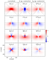 |
Fig. 21 Zero-point correction effects for DiskI60α−2 with a small rin = 0.125DPSF (3.15 mas) and strong unresolved scattering polarization. The panel columns give, from left to right, the polarization maps for the PSFAO convolved disk X(x, y), system-corrected maps Xz(x, y), and center-corrected maps for the extended polarization region Xex(x, y). |
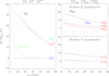 |
Fig. 22 Dependence of the polarization ΣX/Qϕ,ref and quadrant parameters ΣXxxx/Qϕ,ref for DiskI60α−2 as a function of rin for the PSFAO convolved, system-corrected Xz and the center-corrected Xex model parameters. All disks have the same outer boundary of rout = 100.8 mas. For Stokes U quadrants, there is |

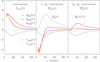 |
Fig. 23 Radial profiles for the polarization signal in the Stokes quadrants for the DiskI60α−2 model with rin = 0.125 DPSF (3.15 mas). The panels give Xxxx(r) for the convolved, |


4.4.2 Quadrant parameters for the extended polarization
The maps for the extended polarization Qex and Uex are useful for the characterization of the azimuthal polarization Qϕ(ϕ). This is illustrated for the DiskI60α−2 models in the right panels of Fig. 22, which show ΣXxxx/Qϕ,ref for the convolved models, and also for the system-corrected  , and center-corrected
  models plotted by black dotted, blue dashed and solid red lines respectively (see also Table E.3).
The behavior of the Q quadrants is very similar to the integrated Stokes parameter ΣQ, with  for rin > DPSF, with a strong increase of ΣQxxx for rin < DPSF, and much lower values for the system-corrected quadrants
  . The Stokes U quadrant values are for all three cases the same because they are not affected by Stokes Q zp-corrections.
The differences between the lines for Q quadrants with xxx = 090, 000 and 180 are the same for the three cases, and this is equivalent to the differential quadrant values (Eq. (35)), which practically do not depend on a polarization offset. Thus, the differential quadrant values and the corresponding information on the azimuthal distribution of Qϕ(ϕ) is preserved by the zp-correction for the central peak.
Central zero. A most important advantage of the center-corrected maps Qex(x, y) is the central zero (Fig. 21) with facilitates for observational data very significantly the splitting of the Qex-signal into quadrant values. This is illustrated in Fig. 23 with radial profiles for the polarization signal Xxxx(r) obtained by averaging azimuthally the polarization signal within the 90◦ wedges of the individual quadrants. The profiles show for small r some sampling noise because of the used finite pixel size of 0.9 mas × 0.9 mas for the model maps.
The strong central Qc signal, which is positive for the convolved map and negative for the map with a system zp-correction, dominates at small r strongly the Qxxx(r) and  profiles. In these cases the determination of quadrant values ΣQxxx and
  depend critically on the splitting of the strong central signal. This can introduce significant uncertainties for AO data with a variable and not exactly axisymmetric PSF core (e.g., Cantalloube et al. 2019). The splitting of the Stokes signal into quadrant values is less critical for the center-corrected Qex map with a signal close to zero in the center, where the borderlines between the quadrants intersect. Therefore, the center zp-correction is very helpful for the derivation of the azimuthal distribution of the Stokes parameters Q(ϕ) and U(ϕ) using quadrant parameters and for the azimuthal parameters Qϕ(ϕ) and Uϕ(ϕ) for barely resolved observational data. This is also supported by recent results for observations of the circumstellar dust around post-AGB stars (Andrych et al. 2024, 2025).
5 Summary and discussion
High resolution imaging polarimetry is a very attractive differential technique for the detection of a circumstellar scattering regions because the produced polarization signal can be separated from the strong radiation of the central star (e.g., Kuhn et al. 2001; Perrin et al. 2004; Hinkley et al. 2009). However, imaging polarimetry is affected by observational convolution effects and by calibration offsets which must be taken into account for a quantitative analysis (e.g., Schmid et al. 2006; Monnier et al. 2019; Hunziker et al. 2021; Tschudi & Schmid 2021; Ma et al. 2024b). This work investigates these effects systematically and provides guide lines for the derivation of quantitative polarimetric results from observational data. Basic effects are treated with simple model simulations using axisymmetric PSFs, considering only axisymmetric or mirror symmetric scattering geometries aligned with the Stokes Q polarization direction, and circular or annular apertures for the determination of zp-correction offsets and integrated flux parameters.
The convolved azimuthal polarization for intrinsically axisymmetric models is also axisymmetric Qϕ(r) and depends on the PSF profile. The mirror-symmetric models RingI60 and DiskI60 for inclined disks have an azimuthal dependence for  and they produce a net Stokes ΣQ signal. The PSF convolution and polarization offsets both change the azimuthal distribution of the signal, which is described by Stokes quadrant polarization parameters ΣXxxx. Because only faint disks are considered ΣId ≲ 0.05 ΣIs a polarimetric offset for Stokes Q is close to axisymmetric q I(x, y) ≈ q I(r) and this changes the four quadrants ΣQxxx practically equally, while the Stokes U signal is not changed by a Stokes Q offset. Observational data are more complex than the presented simple simulations and instrumental effects introduce additional noise, but many basic results of this study are still applicable or approximately valid for the interpretation of real data.
Presence of circumstellar polarization. In all models a net positive azimuthal polarization ΣQϕ > 0 indicates the presence of resolved circumstellar scattering polarization. Measurements of ΣQϕ are ideal for the detection of faint, extended circumstellar scattering regions, because the signal is not biased by pixel to pixel noise and can be summed up for large image areas (Schmid et al. 2006). For observational data one needs to define ΣQϕ detection limits considering spurious signals from PSF variations or systematic instrumental noise (e.g., Cantalloube et al. 2019; Tschudi et al. 2024). According to the presented noise free simulations a measurable ΣQϕ-signal can be obtained for very compact scattering regions down to a separation of about r ≈ DPSF and this has also been achieved for observational data (e.g., Avenhaus et al. 2017; Schmid et al. 2018; Andrych et al. 2025). In addition the ΣQϕ value is not significantly changed by a polarization offset p I(r) because this adds for Qϕ(x, y) only a positive-negative quadrant pattern with practically no net ΣQϕ signal.
Degradation of the Qϕ signal. The PSF convolution degrades the ΣQϕ signal because of the smearing and polarimetric cancellation (Schmid et al. 2006). The effect is particularly strong for small separations from the star and there results practically no net ΣQϕ signal for a scattering regions with separation r ≲ 0.5 DPSF from the star. For resolved but compact scattering regions 0.5 DPSF < r < 5 DPSF the degradation depends strongly on the PSF structure and is about a factor of a few for the PSFAO used in the simulations. For scattering regions at larger separation r ≳ 10 DPSF the ΣQϕ degradation is at a level of about ≈10−30% according to Table 1 and the tables in the appendix. For AO observations with high PSF Strehl ratio of about S ≈ 0.8 or a space instrument with S ≈ 1, the degradation would be closer or comparable to the model results using the Gaussian PSFG.
A measurement of the azimuthal polarization ΣQϕ/ΣI should always include an assessment of the convolution effects based on the observational PSF and provide an estimate or even a derivation of the intrinsic circumstellar polarization  . This allows for individual objects comparisons between results from different observations and enables investigations about temporal variations and the wavelength dependence of the polarized reflectivity (e.g., Ma et al. 2024a,b; Andrych et al. 2025).
The PSFAO convolution of inclined disks introduces a cross talk signal Qϕ → Uϕ, significant differences between the azimuthal polarization Qϕ and the polarized flux P, extended Stokes Q, U polarization halos, and central Stokes signals Q, U for unresolved inner scattering regions. These extended and central Stokes components produce in the azimuthal polarization maps Qϕ(x, y) and Uϕ(x, y) quadrant patterns with practically zero net Qϕ, Uϕ signal, if measured in axisymmetric apertures as illustrated in Figs. 9 and 11.
Stokes polarization parameters. The integrated Stokes parameters ΣQ and ΣU do not depend on the PSF convolution but the smearing leads to a mutual averaging of the polarization between the positive and negative Stokes ΣQxxx or ΣUxxx quadrants toward the mean value ΣQ/4 or ΣU/4, respectively. This changes also the azimuthal distribution Qϕ(ϕ) of the circumstellar polarization in step with the degradation of the integrated ΣQϕ signal. Differential quadrant values expressed relative to ΣQϕ, such as(ΣQxxx − ΣQ/4)/ΣQϕ, are much less changed by the PSF convolution, and therefore they provide for convolved data still strong constraints on the intrinsic azimuthal distribution of  . For complex scattering geometries it is more difficult to account for the mutual averaging effect between the polarization quadrants, but the basic principle is still valid and can be considered for the interpretation of the data.
An unresolved central scattering region can produces a central signal ΣQc, ΣUc with a spatial distribution similar to the PSF. This can be compared with the spatially resolved polarization Q(x, y) and U(x, y) at r ≳ DPSF providing potentially strong constraints on the presence and the radius of a central cavity caused by dust sublimation for accretion disks or dust condensation for shells around mass losing stars.
Polarization offsets and zp-correction. Measurements of Stokes parameters ΣQ, ΣU and quadrant values ΣQxxx, ΣUxxx are often affected by residual polarimetric offsets pres I(x, y) introduced by not so well known amounts of intrinsic stellar polarization, or by interstellar and instrumental polarization. Already, an offset of pres ≳ 0.001 can introduce strong bias effects or even mask the circumstellar polarization signal.
A polarimetric zero point or zp-correction accounts for a fractional Stokes polarization offset ⟨q⟩I(x, y) and ⟨u⟩I(x, y), and this is for many observations a key step to reveal better the circumstellar polarization signal.
A correction offset −⟨q⟩ I(x, y) has for all four Stokes Q quadrants the same impact with practically no change for the differential quadrant values Σ2Qxxx − Σ2Q/4. The same would applies for Stokes U offset, and the corrected Stokes values ΣQz, ΣUz and quadrant  ,
,  can be recalibrated, if accurate determination of the intrinsic ΣQ′ and ΣU′ are available.
A zp-correction does not change significantly the integrated azimuthal polarization ΣQϕ, but it introduces a bias effect for the azimuthal signal distribution  . A negative offset −⟨q⟩ I(x, y) reduces for the RingI60 and DiskI60 models the positive Q090 and Q270 quadrants and makes the negative quadrants Q000 and Q180 even more negative. For Qϕ(ϕ), this is equivalent to a weakening around ϕ ≈ 90◦ and ≈270◦, while the signals around ϕ ≈ 0◦ and ≈180◦ are enhanced. The zp-corrected RingI60 model shows for the quadrant ratio
  a value which is more than 50% enhance when compared to the model without zp-correction (Fig. 19, Table E.1), equivalent to a much enhanced front side brightness. This effect must be taken into account for the derivation of the polarized scattering phase functions for the dust in the disk.
A positive Stokes U offset would enhance the U135 and U315 components and make the negative quadrants U045 and U225 even more negative as shown in Fig. 16 and in principle similar to the case of Stokes Q. However, because the U direction is not aligned with the symmetry of the adopted model geometries an U offset distorts the antisymmetric or symmetric appearance of the U, Uϕ and Qϕ maps.
Important for the zp-correction are well-defined correction region Σzp and different useful cases are illustrated in the sketch in Fig. 24. The reference case is a circumstellar signal without intrinsic stellar polarization and observational polarization offset. A system normalization Σzp = Σ sets the net polarization to zero ΣQz = 0, and introduces for the RingI60 model a negative polarization for the star which compensates the circumstellar signal Σ1Qz = −Σ2Qz.
Practically the same Qz maps are obtained for the same circumstellar model, but “affected” by an offset from interstellar, instrumental or intrinsic stellar polarization. Therefore, the zp-correction is very useful to mitigate offsets and calibration uncertainties, because one can search for an intrinsic Q′(x, y), U′(x, y) model, which matches after convolution and a zp-correction the observed and zp-corrected data despite some undefined offsets.
If other data provide accurate values (ΣQ′, ΣU′) = (ΣQ, ΣU), then one can correct the zp-corrected data and derive Q(x, y), U(x, y) maps without offsets. Alternatively, if the central star can be used as zero polarization standard, then a zp-correction based on the star Σzp = Σ1 provides directly the intrinsic Stokes signal  and
and  .
.
A good solution for coronagraphic observations or data with saturated star is the use of the halo region Σzp = Σ3 for the zp-correction, because the fractional polarization of the smeared signal in the halo approximates well the value for the whole system ⟨q3⟩ ≈ ⟨q⟩. This correction provides then a good match for the reference case Qz3(x, y) ≈ Qz(x, y) outside of the coronagraphic mask (Fig. 24). This procedure requires enough signal and the absence of significant systematic errors in the halo for the determination of ⟨q3⟩, what may be critical for some observations. In addition, one needs also a separate PSF calibration to estimate the smearing degradation of the derived Qϕ signal.
For partially resolved scattering regions a zp-correction based on a few of the brightest pixels of the PSF peak Σzp = Σ0 can be very favorable. This approach splits the signal into two components: (i) an unresolved polarization for the central source Q0, U0 with a spatial distribution similar to the PSF and zero azimuthal polarization ΣQϕ,0 ≈ 0 and (ii) extended polarization maps Qex(x, y), Uex(x, y) and  with a central zero, and quadrant values
  ,
,  constraining the azimuthal distribution of Qϕ(ϕ) down to a separation of r ≈ DPSF. The center correction accounts for offsets introduced by interstellar and instrumental polarization, and for the contributions from the intrinsic polarization of the unresolved, central source. The resulting maps represent the resolved part of the circumstellar polarization signal Qex(x, y) ≈ Qd(x, y) and Uex(x, y) ≈ Ud(x, y).
Conclusions. With the presented model simulations, we have systematically explored the PSF convolution effects and the impact of polarization offsets for the imaging polarimetry of circumstellar scattering regions. The simple models we used are ideal for a description of the basic principles that also apply for more complex systems and should be considered for the planning of new observations and for the interpretation and analysis of observational data. Of importance in this approach is that the observational data can be corrected for the instrumental PSF convolution using PSF calibrations and that polarimetric offsets are corrected with a well-defined zp-correction procedure. In particular, for coronagraphic high-contrast observations, a good PSF calibration and polarimetric measurements for the central bright object with non-coronagraphic exposures could provide higher quality results.
Future instruments may target more demanding objects and effects introduced by non-axisymmetric features in the PSF convolution, and field-dependent polarimetric offsets could significantly affect the data. Analysis procedures considering only axisymmetric PSFs and simple fractional polarization offset may not be sufficient. However, an important first step are investigations of the achievable limits using the procedures discussed in this work for available data, which have barely been started despite the existence of many high quality observations in data archives (e.g., Benisty et al. 2023). Pushing the observational limits and the analysis of data from existing instruments will provide useful insights on the next level of challenges to be considered for future improvements in polarimetric imaging.
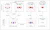 |
Fig. 24 Sketch for the polarimetric zp-corrections procedures for Stokes Q. The system correction Σzp = Σ gives the same Qz for the first two cases, while a star correction Σzp = Σ1 can recover the convolved Qz1 = Q case for data with a polarization offset. A halo correction Σzp = Σ3 is a good approach for coronagraphic data (Qz3 ≈ Qz outside of the coronagraphic disk). A center correction Σzp = Σ0 provides the resolved circumstellar signal Qex for compact regions. |
Acknowledgements
We thank the referee, Frans Snik, for very thoughtful and supportive comments, which improved the manuscript. J.M. thanks the Swiss National Science Foundation for financial support under grant number P500PT_222298.
References
- Andrych, K., Kamath, D., Kluska, J., et al. 2023, MNRAS, 524, 4168 [NASA ADS] [CrossRef] [Google Scholar]
- Andrych, K., Kamath, D., Van Winckel, H., et al. 2024, MNRAS, 535, 1763 [Google Scholar]
- Andrych, K., Kamath, D., Van Winckel, H., et al. 2025, PASA, 42, e125 [Google Scholar]
- Angel, J. R. P., & Martin, P. G. 1973, ApJ, 180, L39 [Google Scholar]
- Arriaga, P., Fitzgerald, M. P., Duchêne, G., et al. 2020, AJ, 160, 79 [Google Scholar]
- Avenhaus, H., Quanz, S. P., Schmid, H. M., et al. 2014, ApJ, 781, 87 [Google Scholar]
- Avenhaus, H., Quanz, S. P., Schmid, H. M., et al. 2017, AJ, 154, 33 [Google Scholar]
- Avenhaus, H., Quanz, S. P., Garufi, A., et al. 2018, ApJ, 863, 44 [NASA ADS] [CrossRef] [Google Scholar]
- Bastien, P., Robert, C., & Nadeau, R. 1989, ApJ, 339, 1089 [Google Scholar]
- Benisty, M., Dominik, C., Follette, K., et al. 2023, ASP Conf. Ser., 534, 605 [NASA ADS] [Google Scholar]
- Beuzit, J. L., Vigan, A., Mouillet, D., et al. 2019, A&A, 631, A155 [NASA ADS] [CrossRef] [EDP Sciences] [Google Scholar]
- Birnstiel, T. 2024, ARA&A, 62, 157 [Google Scholar]
- Canovas, H., Ménard, F., de Boer, J., et al. 2015, A&A, 582, L7 [NASA ADS] [CrossRef] [EDP Sciences] [Google Scholar]
- Cantalloube, F., Dohlen, K., Milli, J., Brandner, W., & Vigan, A. 2019, The Messenger, 176, 25 [NASA ADS] [Google Scholar]
- Chen, C. H., Mittal, T., Kuchner, M., et al. 2014, ApJS, 211, 25 [Google Scholar]
- Crotts, K. A., Matthews, B. C., Duchêne, G., et al. 2024, ApJ, 961, 245 [NASA ADS] [CrossRef] [Google Scholar]
- de Boer, J., Langlois, M., van Holstein, R. G., et al. 2020, A&A, 633, A63 [NASA ADS] [CrossRef] [EDP Sciences] [Google Scholar]
- Draine, B. T. 2003, ARA&A, 41, 241 [Google Scholar]
- Engler, N., Schmid, H. M., Thalmann, C., et al. 2017, A&A, 607, A90 [NASA ADS] [CrossRef] [EDP Sciences] [Google Scholar]
- Esposito, T. M., Kalas, P., Fitzgerald, M. P., et al. 2020, AJ, 160, 24 [Google Scholar]
- Ferrarotti, A. S., & Gail, H. P. 2006, A&A, 447, 553 [CrossRef] [EDP Sciences] [Google Scholar]
- Fétick, R. J. L., Fusco, T., Neichel, B., et al. 2019, A&A, 628, A99 [NASA ADS] [CrossRef] [EDP Sciences] [Google Scholar]
- Garufi, A., Avenhaus, H., Pérez, S., et al. 2020, A&A, 633, A82 [NASA ADS] [CrossRef] [EDP Sciences] [Google Scholar]
- Garufi, A., Dominik, C., Ginski, C., et al. 2022, A&A, 658, A137 [NASA ADS] [CrossRef] [EDP Sciences] [Google Scholar]
- Gáspár, A., Wolff, S. G., Rieke, G. H., et al. 2023, Nat. Astron., 7, 790 [CrossRef] [Google Scholar]
- Ginski, C., Tazaki, R., Dominik, C., & Stolker, T. 2023, ApJ, 953, 92 [NASA ADS] [CrossRef] [Google Scholar]
- Graham, J. R., Kalas, P. G., & Matthews, B. C. 2007, ApJ, 654, 595 [Google Scholar]
- Heikamp, S., & Keller, C. U. 2019, A&A, 627, A156 [NASA ADS] [CrossRef] [EDP Sciences] [Google Scholar]
- Hinkley, S., Oppenheimer, B. R., Soummer, R., et al. 2009, ApJ, 701, 804 [NASA ADS] [CrossRef] [Google Scholar]
- Hodapp, K. W., Suzuki, R., Tamura, M., et al. 2008, SPIE Conf. Ser., 7014, 701419 [Google Scholar]
- Höfner, S., & Olofsson, H. 2018, A&A Rev., 26, 1 [Google Scholar]
- Hughes, A. M., Duchêne, G., & Matthews, B. C. 2018, ARA&A, 56, 541 [Google Scholar]
- Hunziker, S., Schmid, H. M., Ma, J., et al. 2021, A&A, 648, A110 [NASA ADS] [CrossRef] [EDP Sciences] [Google Scholar]
- Hunziker, S., Schmid, H. M., Mouillet, D., et al. 2020, A&A, 634, A69 [NASA ADS] [CrossRef] [EDP Sciences] [Google Scholar]
- Kalas, P., Graham, J. R., Fitzgerald, M. P., & Clampin, M. 2013, ApJ, 775, 56 [NASA ADS] [CrossRef] [Google Scholar]
- Khouri, T., Vlemmings, W. H. T., Paladini, C., et al. 2020, A&A, 635, A200 [NASA ADS] [CrossRef] [EDP Sciences] [Google Scholar]
- Kuhn, J. R., Potter, D., & Parise, B. 2001, ApJ, 553, L189 [NASA ADS] [CrossRef] [Google Scholar]
- Kwon, J., Tamura, M., Hough, J. H., et al. 2014, ApJ, 795, L16 [Google Scholar]
- Lawson, K., Schlieder, J. E., Leisenring, J. M., et al. 2023, AJ, 166, 150 [NASA ADS] [CrossRef] [Google Scholar]
- Lenzen, R., Hartung, M., Brandner, W., et al. 2003, SPIE Conf. Ser., 4841, 944 [Google Scholar]
- Lucas, M., Norris, B., Guyon, O., et al. 2024, PASP, 136, 114504 [Google Scholar]
- Ma, J., & Schmid, H. M. 2022, A&A, 663, A110 [NASA ADS] [CrossRef] [EDP Sciences] [Google Scholar]
- Ma, J., Schmid, H. M., & Tschudi, C. 2023, A&A, 676, A6 [NASA ADS] [CrossRef] [EDP Sciences] [Google Scholar]
- Ma, J., Ginski, C., Tazaki, R., et al. 2024a, A&A, 691, L16 [NASA ADS] [CrossRef] [EDP Sciences] [Google Scholar]
- Ma, J., Schmid, H. M., & Stolker, T. 2024b, A&A, 683, A18 [NASA ADS] [CrossRef] [EDP Sciences] [Google Scholar]
- Milli, J., Vigan, A., Mouillet, D., et al. 2017, A&A, 599, A108 [NASA ADS] [CrossRef] [EDP Sciences] [Google Scholar]
- Milli, J., Engler, N., Schmid, H. M., et al. 2019, A&A, 626, A54 [NASA ADS] [CrossRef] [EDP Sciences] [Google Scholar]
- Monnier, J. D., Harries, T. J., Bae, J., et al. 2019, ApJ, 872, 122 [Google Scholar]
- Montargès, M., Cannon, E., de Koter, A., et al. 2023, A&A, 671, A96 [NASA ADS] [CrossRef] [EDP Sciences] [Google Scholar]
- Murakawa, K., Suto, H., Tamura, M., et al. 2004, PASJ, 56, 509 [NASA ADS] [Google Scholar]
- Ohnaka, K., Weigelt, G., & Hofmann, K. H. 2016, A&A, 589, A91 [NASA ADS] [CrossRef] [EDP Sciences] [Google Scholar]
- Perrin, M. D., Sivaramakrishnan, A., Makidon, R. B., Oppenheimer, B. R., & Graham, J. R. 2003, ApJ, 596, 702 [NASA ADS] [CrossRef] [Google Scholar]
- Perrin, M. D., Graham, J. R., Kalas, P., et al. 2004, Science, 303, 1345 [Google Scholar]
- Perrin, M. D., Duchene, G., Millar-Blanchaer, M., et al. 2015, ApJ, 799, 182 [Google Scholar]
- Pinilla, P., Benisty, M., de Boer, J., et al. 2018, ApJ, 868, 85 [NASA ADS] [CrossRef] [Google Scholar]
- Poteet, C. A., Chen, C. H., Hines, D. C., et al. 2018, ApJ, 860, 115 [Google Scholar]
- Quanz, S. P., Schmid, H. M., Geissler, K., et al. 2011, ApJ, 738, 23 [Google Scholar]
- Quanz, S. P., Avenhaus, H., Buenzli, E., et al. 2013, ApJ, 766, L2 [Google Scholar]
- Rapson, V. A., Kastner, J. H., Millar-Blanchaer, M. A., & Dong, R. 2015, ApJ, 815, L26 [Google Scholar]
- Ren, B. B., Benisty, M., Ginski, C., et al. 2023, A&A, 680, A114 [NASA ADS] [CrossRef] [EDP Sciences] [Google Scholar]
- Schmid, H. M. 2021, A&A, 655, A83 [NASA ADS] [CrossRef] [EDP Sciences] [Google Scholar]
- Schmid, H. M. 2022, arXiv e-prints [arXiv:2207.14511] [Google Scholar]
- Schmid, H. M., Joos, F., & Tschan, D. 2006, A&A, 452, 657 [NASA ADS] [CrossRef] [EDP Sciences] [Google Scholar]
- Schmid, H. M., Bazzon, A., Roelfsema, R., et al. 2018, A&A, 619, A9 [NASA ADS] [CrossRef] [EDP Sciences] [Google Scholar]
- Schneider, G., Grady, C. A., Hines, D. C., et al. 2014, AJ, 148, 59 [NASA ADS] [CrossRef] [Google Scholar]
- Simmons, J. F. L., & Stewart, B. G. 1985, A&A, 142, 100 [NASA ADS] [Google Scholar]
- Stolker, T., Dominik, C., Avenhaus, H., et al. 2016, A&A, 595, A113 [NASA ADS] [CrossRef] [EDP Sciences] [Google Scholar]
- Tinbergen, J. 2007, PASP, 119, 1371 [NASA ADS] [CrossRef] [Google Scholar]
- Tschudi, C., & Schmid, H. M. 2021, A&A, 655, A37 [NASA ADS] [CrossRef] [EDP Sciences] [Google Scholar]
- Tschudi, C., Schmid, H. M., Nowak, M., et al. 2024, A&A, 687, A74 [NASA ADS] [CrossRef] [EDP Sciences] [Google Scholar]
- van Boekel, R., Henning, T., Menu, J., et al. 2017, ApJ, 837, 132 [Google Scholar]
- van Holstein, R. G., Girard, J. H., de Boer, J., et al. 2020, A&A, 633, A64 [NASA ADS] [CrossRef] [EDP Sciences] [Google Scholar]
- Woitke, P., Kamp, I., Antonellini, S., et al. 2019, PASP, 131, 064301 [NASA ADS] [CrossRef] [Google Scholar]
- Zhou, Y., Bowler, B. P., Yang, H., et al. 2023, AJ, 166, 220 [NASA ADS] [CrossRef] [Google Scholar]
Defined as in the FORTRAN function atan2(y,x) for Cartesian to polar coordinate conversions.
This convolution cross talk is different from instrumental polarization cross talks which are introduced by optical components (e.g., Tinbergen 2007).
Appendix A Polarization parameters
Stokes polarization parameters Q, U and azimuthal polarization parameters Qϕ, Uϕ are used in this work for the description of the model results. Convolution and polarization offset are simple mathematical operations for the Stokes parameters, but quite complex for the azimuthal parameters. Therefore, a comprehensive quantitative description of the circumstellar scattering polarization requires an extensive framework of parameters, which is outlined in Table A.1 for the convolved models and in Table A.2 for zp-corrected models in the system aligned x, y coordinates.
Here we give a few remarks on the entries in the tables. The integration regions, Σint, and the zp-calibration regions, Σzp, are defined on a model-by-model basis. The aim is to quantify the polarization signal for the whole system, Σ, only the central source, Σ1; the disk, Σ2; and the halo, Σ3, or a combination of these subregions, such as Σ1+2.
It is also important to distinguish between ΣP and (Σ). ΣP is the sum of the degree of linear polarization measured for each pixel in the resolved map in the integration region Σ (Eq. 10). This is not considering the position angle θ of the polarization. In addition, the polarization ΣP depends in a complex way on the spatial resolution, on instrumental noise, and on polarization offsets.
Therefore it is useful to characterize the “aperture” polarization (Σi) for a given integration region Σi using the sums of the Stokes parameters according to
 (A.1)
with the corresponding position angle
(A.1)
with the corresponding position angle
 (A.2)
(A.2)
The fractional polarization can then be defined by pi = (Σi)/ΣiI or for the Stokes components by qi = ΣiQ/ΣiI and ui = ΣiU/ΣiI, from which one can also derive a position angle θi. The polarization of the star, or all the fractional polarization parameters like qis, ⟨qi⟩, or q0, are defined with these “aperture” polarization parameters.
Appendix B Faint PSFAO artifacts
The extended halo of the PSFAO, in particular the strong speckle ring at a separation of about 0.45″, can introduce weak artifacts in the convolved polarization maps. For an axisymmetric, compact system with r0 < 100 mas the positive-negative Stokes Q and U quadrant patterns are not resolved by the PSF halo, and therefore there is no net ΣQ and ΣU signal that can produce a polarized halo ghost signal. However, for more extended scattering regions the quadrant patterns are also resolved by the PSF halo and this can produce various kinds of weak spurious features.
One example is illustrated in Fig. B.1 for the Ring0 model with r0 = 201.6 mas convolved with PSFAO, but also with PSF1 representing the full 2D speckle structure of a single frame from SPHERE/ZIMPOL (see Schmid et al. 2018, for PSF details). If multiple polarimetric measurements are taken in field rotation mode and then combined in a derotated dataset, then the patterns in PSF1 will average toward the case PSFAO. The panels in Fig. B.1 emphasize the weak outer structure in the convolved Qϕ(x, y) and Q(x, y), U(x, y) maps using a strongly saturated color scale. The insets on the lower right show the central ring signals with a 200 × wider color scale.
The PSFAO speckle ring, indicated in Fig. B.1 for the PSFs by a dashed circle, produces in the Stokes maps for the positive or negative Stokes quadrants of the circumstellar polarization ring, a corresponding circular positive and negative ghost on top of the disk signal. This is indicated in the U(x, y) maps with four dashed circles centered on the U ring quadrants. These ghosts add up to a weak positive/negative tile pattern for the convolution with PSF1 with its quadratic substructure, while the pattern is much smoother for the PSFAO convolved U maps. The same ghosts, but rotated by 45◦, are present in the Stokes Q maps. Therefore, there results for the convolved Qϕ(x, y) map a weak, negative ring (a radial polarization signal!) just outside the disk ring, and a weak positive ring further out. This is a special case because the polarization is concentrated in a narrow ring with a radius of about half the size of the PSFAO speckle ring. The surface brightness of the spurious negative Qϕ-signal at r ≈ 460 mas is at the level of −0.2 % of the positive Qϕ surface brightness peak signal of the disk ring. The negative Qϕ signal introduces also a small discrepancy between the integrated ΣQϕ and ΣP values despite the strict axisymmetry.
Polarization parameters for convolved and intrinsic models.
Polarization parameter for the zp-corrected models.
Another type of circular ghost pattern appears for the large Ring0 model with r0 ≈ 800 mas, where the PSFAO convolution produces two weak, positive Qϕ ghost rings, one just outside and one just inside of the bright disk ring. These features are also very faint and can often be neglected in typical polarimetric data taken with current AO systems. However, one should be careful with the interpretation of faint structures near bright scattering regions. The protoplanetary disk around HD 169142 is a case with a narrow bright ring, where this type of ghost had to be taken into account in the measurements of Tschudi & Schmid (2021) for the determination of the faint signal from the disk region located further out.
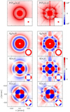 |
Fig. B.1 Faint polarization artifacts in the maps Qϕ(x, y), Q(x, y), U(x, y) of the Ring0 model r0 = 201.6 mas produced by the axisymmetric PSFAO(x, y) (left column) and a 2D single-frame speckle PSF1 of an AO system (right column). Dashed circles are indicated for the PSFs and the Stokes U maps to indicate the location of the halos produced by the speckle ring. The color scale is strongly saturated in the center of the main maps, and therefore this region is plotted as inset in the lower right with a 200 times wider color scale. |
Appendix C Parameters for Disk0 models
Table C.1 gives numerical values for the simulation of the axisymmetric, extended models Disk0α0, Disk0α−1, and Disk0α−2 described in Sect. 3.1.2. For all models with the same α-index the intrinsic  , and the PSFG and PSFAO convolved ΣQϕ values are given relative to the reference value
  .
.
The intrinsic  value for the Disk0α0 model with a flat surface brightness plotted in Fig. 7 does not change much between rin = 0 and 0.5 DPSF. For the convolved signal there is almost no difference in
  for rin ≲ DPSF and one cannot distinguish easily between different rin cases. One can use the hole radius rh(Qϕ) to distinguish between models with rin = 0.5 DPSF and 1.0 DPSF, but this would require for observational studies high quality data.
For the Disk0α−2 the intrinsic  signal for a small cavity rin = 0.125 DPSF is much larger than the reference value, because the brightness increases rapidly toward the center (see Fig. 8). For the convolved signal
  the contributions from the central disk regions are strongly suppressed by polarimetric cancellation, but there is still a difference of about 20 % to 30 % between the model with rin = 0.5 DPSF and 1.0 DPSF. Also the radii r(max(Qϕ)) and rh(Qϕ) are quite different between these two cases. For the Disk0α−1 models these relative differences are intermediate between Disk0α0 and Disk0α−2.
Results for the axisymmetric models Disk0α0, Disk0α−1, and Disk0α−2.
Appendix D Parameters for inclined disks
D.1 RingI60 models
Results of the RingI60 simulations discussed in Sect. 3.2 are listed in Table D.1. All values for the integrated polarization parameters are normalized  to the intrinsic azimuthal polarization with X = {Qϕ, Q, P, |Qϕ|, |Uϕ|, |Q|, |Q|}.
The same normalization is applied to the five quadrant polarization values  with Xxxx = {Q000, Q090, Q180, U045, U135}. Also given is the ratio between Σ|Uϕ|/Σ|Qϕ| as measure for the Qϕ → Uϕ convolution cross talk. The values in Table D.1 were numerically integrated for an aperture with r = 1.5″.
The first line in Table D.1 gives the values for the intrinsic model and the second line for a convolved but spatially unresolved RingI60 model. For Σ|Qϕ| and Σ|Uϕ| of the unresolved model the value (2/π) ΣQ is given, which follows from the analytic solution for the azimuthal integration of Qϕ(ϕ) = −Q cos(2ϕ) and Uϕ = −Q sin(2ϕ) of a “perfect” quadrant pattern for a PSF convolved point source with a polarization Q
The  -values for the PSFG and PSFAO convolved models with different r0 correspond to the diagrams in Fig. 10, while the curves for the quadrant values
  are shown in the upper panels of Fig. 13.
For the PSFAO convolved model with r0 = 50.4 mas not only values for an aperture with r = 1.5″ are given, but also the splitted values for the disk region using a circular aperture with r = 0.2″ and for the halo region using an annular aperture from r = 0.2″ to 1.5″. These values are given to support the discussion of the weak halo signal in Sect. 3.2.2 and Fig. 11.
The numerical integration of the polarization fluxes is affected for the smallest rings by the limited spatial sampling of 0.9 mas × 0.9 mas per pixel. This produces errors larger than two units in the last indicated digit for some tabulated values for the PSFG convolved model with r0 = 3.15 mas and for the PSFAO convolved model with r0 = 6.3 mas.
Smearing for PSFAO convolved models puts some flux outside of the aperture radius r = 1.5″. The strength of this effect follows from convolved small disk models r0 ≤ 201.6 mas which give  instead of the intrinsic value 42.1 %. For extended disks with r0 > 200 mas additional disk polarization is “lost” outside the aperture because of the convolution.
The differential Stokes quadrant values ∆Q000, ∆Q090, ∆Q180, and ∆U+ are listed in Table D.2. They are expressed as ratio relative to ΣQϕ for the RingI60 models with different r0 based on the values given in Table D.1. They are derived according to the Eqs. 15 and 17 and are also plotted in the lower panels of Fig. 13.
D.2 DiskI60 models
Table D.3 gives integrated polarization parameters for the extendend, i = 60◦ inclinded disk models DiskI60α0, DiskI60α−1, and DiskI60α−2 for different cavity sizes rin. The outer disk radius is in all cases rout = 100.8 mas. The model with rin = 0.5 DPSF (12.6 mas) represents for all models with the same α-index the reference value  (rin = 0.5 DPSF) as in Table C.1.
The model parameters α, rin, and rout for the inclined disks corresponds to Table C.1 for pole-on models, except for the disk inclination. Therefore, the intrinsic polarization values  are practically the same apart for some numerical sampling errors for disks with bright (α = −2) and barely resolved (rin < 0.5 DPSF) inner regions. For the selected disk inclination the ratio
  is for all intrinsic models 0.421. The Stokes value ΣQ is not changed by the convolution ΣQ/ΣQ′ = 1, but for the PSFAO convolved results this value is ΣQ/ΣQ′ = 0.98 because a small amount of the smeared Q-signal is located outside the used aperture with r = 1.5″.
The values for  and ΣP are plotted for convolved DiskI60α−2 models in Fig. 15 as a function of rin. Of interest is the ratio ΣQϕ/ΣQ, which depends on the cancellation of the Qϕ signal in particular for bright, barely resolved inner disk regions. Table D.3 gives the values for this dependence also for the models DiskI60α0 and DiskI60α−1.
The convolved polarized flux ΣP differs for DiskI60 models significantly from ΣQϕ, unlike for the pole-on models where ΣP ≈ ΣQϕ. The polarized flux ΣP represents a complex mix (Eq. 10) of the azimuthal polarization Qϕ and Uϕ or of the Stokes Q and U components.
Appendix E ZP-corrected disk models
E.1 RingI60 model with r0 = 100.8 mas
Table E.1 lists polarization parameters Qϕ, Q, P and Stokes Q quadrant values Q000, Q090, Q180 for the RingI60 models with r0 = 100.8 mas. Results for many combination of used regions for the zp-correction Σzp and integration regions Σint are given as described in Sects. 4.3.1 and 4.3.2 and partly shown in Figs. 18 and 19.
Results for RingI60 models with different r0.
Differential quadrant values ∆Qxxx and ∆U+ for RingI60 models.
The integration apertures are defined as follows: round apertures Σ with r ≤ 1.5″ for the entire system and Σ1 with r ≤ 0.027″ for the star, and annular aperture Σ2 with 0.027″ < r ≤ 0.2″ for the disk region and Σ3 with 0.2″ < r ≤ 1.5″ for the halo. There is Σ1 + Σ2 + Σ3 = Σ. All polarization values in Table E.1 are given relative to  .
.
The first line gives values for the intrinsic model which are identical to the first line in Table D.3, where also the Stokes U quadrant values  and
and  are given. For the intrinsic model the values for Σ2 are identical to the system values Σ, because the polarization signal in Σ1 and Σ3 are zero.
The lines 2 to 5 in Table E.1 list the polarization for the PSFAO convolved RingI60 model for different integration regions Σi. The values for Σ are identical to entries in the fourth last line of Table D.3, which gives also the Stokes U quadrant values  and
and  . The values for the halo are
  ,
,  , while they are zero for the Σ1 region. The values for Σi = Σ1, Σ2, and Σ3 show how the convolution changes the distribution of the polarization radially.
The following lines in Table E.1 give the same parameters as for the convolved model, but after zp-correction using different reference regions Σzp = Σ, Σ1, Σ2, Σ2+3 and Σ3. It is obvious that the different zp-correction offsets change strongly the values for ΣiQ, ΣiP, and the Stokes quadrants ΣiQxxx.
Results for the DiskI60α0, DiskI60α−1, and DiskI60α−2 models.
An important result is, that the azimuthal polarization  is practically not changed by the applied correction offsets. Also the Stokes U quadrant values are not changed because only offsets for the Stokes Q polarization component are applied in these simulations. The Q quadrant values
  ,
,  , and
, and  for the halo region have after a zp-correction practically the same value, because all quadrants are offset by the same amount. The same also applies roughly for the Stokes Qz quadrants integrated in the stellar aperture Σi = Σ1.
E.2 ZP-corrected model RingI60 with r0 = 403.2 mas
Table E.2 gives polarization parameters for the very large RingI60 model with r0 = 403.2 mas of Fig. 20 in Sect. 4.3.3, and they quantify the impact of different zp-correction for a disk with r0 similar to the radius of the PSF speckle ring of an AO-system.
The first line in Table E.2 gives values identical to the second last line of Table D.1, where also the ΣUxxx quadrant parameters for this model are given. The values for Σint = Σ1, Σ2, and Σ3 give the radial distribution of the PSFAO-convolved polarization signal. The integration regions are defined by the circular aperture r ≤ 0.1″ for Σ1 representing the star or the coronagraphic mask, and by the annular apertures 0.1″ < r ≤ 0.5″ for Σ2 and 0.5″ < r ≤ 1.5″ for Σ3. For the Stokes U quadrants there is  and
and  , the corresponding Σ1 values are zero and the Σ3 values are the differences between the Σ and Σ2 values. The distribution of the intensity
  in the PSFAO convolved images are 66.2 %, 13.5 % and 18.1 % for the integration regions Σ1, Σ2 and Σ3, respectively. The intrinsic disk signal is
  and
and  .
.
Results for the RingI60 models with r0 = 100.8 mas using different zp-corrections.
The last five lines in Table E.2 give the polarization values for the disk aperture Σi = Σ2 after zp-correction in different apertures Σzp. The Σ2Uxxx values given above for the convolved model are not changed by a Stokes Q zp-correction.
The ideal case is the zp-correction using the unpolarized star signal in Σzp = Σ1, which yields the same result as the (initial) PSFAO convolved model. For coronagraphic observations a zp-correction including the Σ1 region is not possible. The Σzp = Σ2 correction sets the Stokes Σ2Q signal to zero and this introduces for this model a very large polarization offset. Using the halo for the zp-correction Σzp = Σ3 is practically equivalent to the case Σzp = Σ for a total system correction, which is a good approach to account for undefined instrumental polarization effects, which may be re-calibrated with aperture polarimetry. A Σ or system zp-correction means also ΣQz = 0 ≈ Σ3Qz and Σ2Qz ≈ −Σ1Qz (Table E.1). Measuring the halo polarization signal can be problematic, if the halo signal is noisy. A zp-correction based on a region including disk and halo regions Σzp = Σ2+3 is also problematic because this depends on the PSF-convolution.
Comparison for different zp-corrections for the extended model RingI60 with r0 = 403.2 mas.
For all Σzp regions practically the same azimuthal polarization Σ2Qϕ is obtained, emphasizing the important invariance of ΣQϕ with respect to polarization offset. Of course, this property is based on the use of an axisymmetric PSF and axisymmetric integration regions in the simulations. Contrary to this, the integrated polarization Σ2P changes by the use of different integration region by up to about 20 %, and this does not include the problem of the noise bias, which might be very significant for observations of extended, low surface brightness scattering regions.
E.3 Center-corrected DiskI60α-2 models
The Table E.3 gives numerical values for the PSFAO convolved DiskI60α−2 models, and for center-corrected Σzp = Σ0 and system-corrected Σzp = Σ models. For the size of the inner disk cavity the two cases rin = 0.125 DPSF (3.15 mas) and rin = 0.5 DPSF (12.6 mas) were selected. The latter case is the reference disk with  for the intrinsic azimuthal polarization. For the model with the small cavity the intrinsic polarization
  is much larger when compared to Qref, but most of the additional azimuthal polarization is not resolved (see Table D.3). Also the ΣQ signal is high for the rin = 0.125 DPSF model and Fig. 21 shows the PSFAO convolved polarization maps X(x, y) for X = {Q, U, Qϕ, Uϕ}, and the resulting maps after a system zp-correction Xz and a center zp-correction Xex. The integration regions Σi are defined by round apertures r ≤ 1.5″ for the whole system Σ, and r ≤ 0.2″ for the star and disk region Σ1+2, and by an annular aperture 0.2″ < r ≤ 1.5″ for the halo region Σ3.
Comparison of values for two compact DiskI60α−2 models without and with two types of zp-correction.
The system zp-correction Σzp = Σ sets the ΣQ signal to zero and this reduces for both rin cases strongly the ΣQxxx quadrant values. The center-corrected values for the disk with the small cavity rin = 0.125DPSF are very similar (within 15 %) to the case of the reference model with a cavity size of rin = 0.5DPSF. Thus, the center zp-correction accounts practically for the Stokes Q polarization offset introduced by the unresolved central region. This correction offset is  for the model with rin = 0.125DPSF and 3.9 % for rin = 0.5DPSF. The quadrant values for U045 and U135 are practically unchanged for a zp-correction of a Stokes Q polarization.
All Tables
Results for the RingI60 models with r0 = 100.8 mas using different zp-corrections.
Comparison for different zp-corrections for the extended model RingI60 with r0 = 403.2 mas.
Comparison of values for two compact DiskI60α−2 models without and with two types of zp-correction.
All Figures
|
Fig. 1 Block diagram with the simplified description of the simulated imaging polarimetry given in blue. The red arrows show the full imaging process from the intrinsic model to the on-sky model including interstellar polarization to the observed and possibly zp-corrected polarization signal. |
| In the text | |
|
Fig. 2 Maps for the intrinsic disk intensity |
| In the text | |
|
Fig. 3 Radial profiles for the extended PSFAO (red) and the Gaussian PSFG (black). In the main panel, the total flux is normalized to 106 counts. In the inset, PSFG is reduced by a factor of 0.4 for a comparison of the PSF cores. The pixel size is 3.6 mas × 3.6 mas. |
| In the text | |
|
Fig. 4 Maps for the Ring0 models with r0 = 12.6 mas (left), 25.2 mas (middle), and 50.4 mas (right) for the intrinsic circumstellar intensities, |
| In the text | |
|
Fig. 5 Normalized radial profiles for the intrinsic |
| In the text | |
|
Fig. 6 Central cancellation holes in the Qϕ(x, y) maps for the models Disk0α0, Disk0α−1, and Disk0α−2 after convolution with the extended PSFAO. The size of the inner cavity rin = 0.125DPSF (3.15 mas) is the same for all three models and indicated by the black dot. |
| In the text | |
|
Fig. 7 Normalized profiles |
| In the text | |
|
Fig. 8 Radial profiles Qϕ(r) for the Disk0α−2 model convolved with PSFAO on a log-scale (upper panel) and a linear scale (lower panel) for different inner cavities r0 as indicated by the colors. The thin black line is the intrinsic surface brightness |
| In the text | |
|
Fig. 9 Maps for the intensity Id and polarization Qϕ, Q, U, Qϕ, Uϕ, and P (from top to bottom) for RingI60 models with r0 = 12.6 mas, 25.2 mas, and 50.4 mas after convolution with the Gaussian PSFG (first three columns). The last column gives the same for the intrinsic model with r0 = 50.4 mas. Stokes quadrant parameters are indicated in some Q and U maps. |
| In the text | |
|
Fig. 10 Integrated polarization parameters for the RingI60 model as a function of the ring radius r0 after convolution with PSFG (a) and PSFAO (b). All parameters have been normalized to the intrinsic value |
| In the text | |
|
Fig. 11 Large-scale halo signals for the Stokes parameters Q, U and the azimuthal polarization Qϕ(x, y), Uϕ(x, y) for the RingI60 model with r0 = 50.4 mas convolved with PSFAO. The inset on the lower-right in each panel shows the disk ring in the center with a color scale reduced by 500 times. |
| In the text | |
|
Fig. 12 Azimuthally averaged profiles for Qϕ(r), |Qϕ(r)|, and |Uϕ(r)| for the RingI60 models with r0 = 25.2 mas and 201.6 mas convolved with PSFAO. The green curve for the ratio |Uϕ(r)|/|Qϕ(r)| provides a rough measure for the convolution cross talk, and the dashed line indicates the system integrated value Σ|Uϕ|/Σ|Qϕ| from Table D.1. |
| In the text | |
|
Fig. 13 Quadrant polarization parameters ΣXxxx normalized to the intrinsic azimuthal polarization |
| In the text | |
|
Fig. 14 Intrinsic maps |
| In the text | |
|
Fig. 15 Integrated polarization parameters ΣQϕ, ΣP, ΣQd for the inclined DiskI60α−2 model as a function of the radius of the inner cavity rin and for PSFG and PSFAO convolution. All values have been normalized to the intrinsic value |
| In the text | |
|
Fig. 16 Polarization maps Q, U, Qϕ, Uϕ for the model DiskI60α−2 (rin = 0.5 DPSF or 12.6 mas) and a polarized central star with |
| In the text | |
|
Fig. 17 Azimuthally averaged intensity profiles for the disk, Id(r); the star, Is(r); and the total, I(r), for the disk polarization, Qϕ(r), and the intrinsic stellar polarization, psIs(r), or interstellar polarization, pisI(r), introduced by a fractional offset of p = 0.1%. The same disk model, polarization offset psIs(r), and PSFAO convolution as in Fig. 16 is used, while the interstellar offset for pisI(r) is applied to the total intensity. |
| In the text | |
|
Fig. 18 Polarization maps for the RingI60 model with r0 = 100.8 mas convolved with PSFAO. The columns shows, from left to right, the convolved maps X(x, y), the maps Xz(x, y) for a system zp-correction, and Xz2(x, y) for disk zp-correction. The circles describe the integration regions Σ1, Σ2, and Σ3 as indicated in the Qϕ(x, y) panel and quadrant regions Σ2Xxxx are identified in the Q(x, y) and U(x, y) panels. |
| In the text | |
|
Fig. 19 Relative quadrant polarization parameters Σ2Xxxx (♢) and their azimuthal values Σ2Xxxx|ϕ (horizontal bars) for the disk integration region Σ2 for RingI60 with r0 = 100.8 mas: (a) instrinsic model, (b) convolved model, (c) Σ corrected model, and (d) Σ2 corrected model. The green and grey lines in (b) indicate the change of Σ2Xxxx and Σ2Xxxx|ϕ, respectively, with respect to panel a, and in the panels c and d with respect to panel b. All vallues are normalized to |
| In the text | |
|
Fig. 20 Effects of the zp-correction for Stokes Q for the PSFAO convolved RingI60 model with r0 = 403.2 mas for observations with a coronagraphic mask, indicated by the central hatched area. Panel a shows the convolved signal Q(x, y), b shows the map after a correction based on the halo Qz3, c shows the map after correction based on the disk plus halo Qz2+3, and d shows the map after correction based on the disk region Qz2. The peak Q signal is in all panels between 22 and 23 units with respect to the indicated color scale. |
| In the text | |
|
Fig. 21 Zero-point correction effects for DiskI60α−2 with a small rin = 0.125DPSF (3.15 mas) and strong unresolved scattering polarization. The panel columns give, from left to right, the polarization maps for the PSFAO convolved disk X(x, y), system-corrected maps Xz(x, y), and center-corrected maps for the extended polarization region Xex(x, y). |
| In the text | |
|
Fig. 22 Dependence of the polarization ΣX/Qϕ,ref and quadrant parameters ΣXxxx/Qϕ,ref for DiskI60α−2 as a function of rin for the PSFAO convolved, system-corrected Xz and the center-corrected Xex model parameters. All disks have the same outer boundary of rout = 100.8 mas. For Stokes U quadrants, there is |
| In the text | |
|
Fig. 23 Radial profiles for the polarization signal in the Stokes quadrants for the DiskI60α−2 model with rin = 0.125 DPSF (3.15 mas). The panels give Xxxx(r) for the convolved, |
| In the text | |
|
Fig. 24 Sketch for the polarimetric zp-corrections procedures for Stokes Q. The system correction Σzp = Σ gives the same Qz for the first two cases, while a star correction Σzp = Σ1 can recover the convolved Qz1 = Q case for data with a polarization offset. A halo correction Σzp = Σ3 is a good approach for coronagraphic data (Qz3 ≈ Qz outside of the coronagraphic disk). A center correction Σzp = Σ0 provides the resolved circumstellar signal Qex for compact regions. |
| In the text | |
|
Fig. B.1 Faint polarization artifacts in the maps Qϕ(x, y), Q(x, y), U(x, y) of the Ring0 model r0 = 201.6 mas produced by the axisymmetric PSFAO(x, y) (left column) and a 2D single-frame speckle PSF1 of an AO system (right column). Dashed circles are indicated for the PSFs and the Stokes U maps to indicate the location of the halos produced by the speckle ring. The color scale is strongly saturated in the center of the main maps, and therefore this region is plotted as inset in the lower right with a 200 times wider color scale. |
| In the text | |
Current usage metrics show cumulative count of Article Views (full-text article views including HTML views, PDF and ePub downloads, according to the available data) and Abstracts Views on Vision4Press platform.
Data correspond to usage on the plateform after 2015. The current usage metrics is available 48-96 hours after online publication and is updated daily on week days.
Initial download of the metrics may take a while.