| Issue |
A&A
Volume 706, February 2026
|
|
|---|---|---|
| Article Number | A113 | |
| Number of page(s) | 9 | |
| Section | Catalogs and data | |
| DOI | https://doi.org/10.1051/0004-6361/202556381 | |
| Published online | 09 February 2026 | |
A survey for radio pulsars and transients in the 10 pc region around Sgr A*
1
Max-Planck-Institut für Radioastronomie,
Auf dem Hügel 69,
53121
Bonn,
Germany
2
National Astronomical Observatories, Chinese Academy of Sciences,
20A Datun Road, Chaoyang District,
Beijing
100101,
PR China
3
INAF – Osservatorio Astronomico di Cagliari,
Via della Scienza 5,
09047
Selargius
(CA),
Italy
4
Jodrell Bank Centre for Astrophysics, Department of Physics and Astronomy, The University of Manchester,
Manchester
M13 9PL,
UK
5
State Key Laboratory of Radio Astronomy and Technology, Shanghai Astronomical Observatory, CAS,
80 Nandan Road,
Shanghai
200030,
PR China
6
Kavli Institute for Astronomy and Astrophysics, Peking University,
Beijing
100871,
PR China
7
Instituto de Radioastronomía Milimetrica,
Avda. Divina Pastora 7, Núcleo Central,
18012
Granada,
Spain
★ Corresponding author: This email address is being protected from spambots. You need JavaScript enabled to view it.
Received:
11
July
2025
Accepted:
8
December
2025
Abstract
Here we report on a new survey for pulsars and transients in the 10 pc region around Sgr A∗ using the Effelsberg radio telescope at frequencies between 4 and 8 GHz. Our calibrated full-Stokes data were searched for pulsars and transients using PULSARX, TRANSIENTX, and PRESTO. Polarisation information is used in the scoring of the candidates. Our periodicity acceleration and jerk searches allowed us to maintain good sensitivity towards binary pulsars in ≳10-h orbits. In addition, we performed a dedicated search in linear polarisation for slow transients. While our searches yielded no new discovery beyond the redetection of the magnetar SGR J1745−2900, we report on a faint single pulse candidate in addition to several weak periodicity search candidates. After thoroughly assessing our survey’s sensitivity, we determined that it is still not sensitive to a population of millisecond pulsars. Next generation radio interferometers can overcome the limitations of traditional single-dish pulsar searches of the Galactic Centre.
Key words: methods: data analysis / pulsars: general / galaxy: center
© The Authors 2026
 Open Access article, published by EDP Sciences, under the terms of the Creative Commons Attribution License (https://creativecommons.org/licenses/by/4.0), which permits unrestricted use, distribution, and reproduction in any medium, provided the original work is properly cited.
This article is published in open access under the Subscribe to Open model.
Open Access funding provided by Max Planck Society.
1 Introduction
The timing of a radio pulsar in a sufficiently close orbit (orbital period Pb ≲ 1 yr) around Sagittarius A* (Sgr A∗) – the super-massive black hole at the heart of our Galaxy – promises unrivalled tests of gravitational physics (Liu et al. 2012) and would allow for complimentary constraints on the results from the Event Horizon Telescope (EHT) and the GRAVITY experiment at the Very Large Telescope Interferometer (Psaltis et al. 2016). It was demonstrated recently that pulsars with slightly larger orbital periods, Pb ∼ 2–5 yr, are also useful to measure the black hole spin to good precision (Hu & Shao 2024).
For these reasons, the Galactic Centre (GC) has been the subject of numerous pulsar surveys over the past few decades. Despite this (see e.g. Kramer et al. 2000; Klein 2005; Macquart et al. 2010), only five slow pulsars were found in the GC region until 2013; all with a projected distance >25 pc from Sgr A∗ (Johnston et al. 2006; Deneva et al. 2009). Wharton et al. (2012) predicted up to about 100 canonical pulsars (i.e. with spin period Ps of order 0.1–1 s ) and 1000 recycled pulsars (i.e. with spin Ps ≲ 30 ms ) in the central parsec of the GC. The GC could also harbour several recycled pulsars in binary orbits with stellar mass black hole companions (Faucher-Giguère & Loeb 2011). As described above, none of the past surveys detected a pulsar closer than 25 pc in projection from Sgr A∗. Nominally “hyper-strong” scattering towards the GC was blamed for this lack of detection, with an estimated scattering time τ1GHZ of about 1000 s at 1 GHz (Cordes & Lazio 2002). Assuming a Kolmogorov spectrum with spectral index α = −4.4, the scattering time would scale as τ ∼ f α prohibiting any detection of a millisecond-duration pulsed signal at frequencies below ∼10 GHz.
This explanation has come under debate since the discovery of an X-ray outburst and pulsations from the magnetar SGR J1745–2900 (Kennea et al. 2013) and eventually the detection of radio pulsations just a few days later (Eatough et al. 2013). Magnetars are short-lived, slowly-spinning neutron stars whose emissions are powered by the rapid decay of their large, twisted magnetic fields (Kaspi & Beloborodov 2017). With a projected distance of only 2.4 arcsec (Rea et al. 2013), a dispersion measure (DM; the integrated free electron column density along the line of sight) of 1778 pc cm−3, and a rotation measure (RM; the rotation in the plane of polarisation of emission due to an external magnetic field) of −66 960 rad m−2 at the time of discovery (Eatough et al. 2013), this magnetar is thought to be within the Bondi–Hoyle accretion limit of Sgr A∗. Measurements of the scattering time of SGR J1745–2900’s pulsed emission (Spitler et al. 2014) revealed an unexpectedly small scattering time of τ1GHZ = 1.3 ± 0.2 s, compared to the hyper-strong scattering predicted by the NE2001 model (Cordes & Lazio 2002). This result implies a scatter broadening time between 7 ms and 0.5 ms at observing frequencies between 4 and 8 GHz, respectively, potentially hindering the detection of millisecond pulsar (MSP) with Ps below 10 ms but allowing for the detection of non-fully-recycled (Ps ≳ 10 ms) MSPs. And despite more recent surveys with increased sensitivity to both canonical and recycled pulsars (Wharton 2017; Suresh et al. 2022; Torne et al. 2021; Eatough et al. 2021; Torne et al. 2023), no new pulsars with Ps ≲ 1 s have been found within the 25 pc region around Sgr A∗. Dexter & O’Leary (2014) interpreted this discrepancy as possible evidence that the massive stars in the GC predominantly form magnetars instead of canonical pulsars.
We report here on new observations of the GC region (Section 2) intended to better constrain the GC pulsar population. We describe our search pipeline for pulsar and transients in Section 3 and discuss the results of this work in Section 4. We present our conclusions in Section 5.
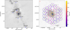 |
Fig. 1 Left panel: image of the GC region produced by MeerKAT at 1.28 GHz (Heywood et al. 2022) with the positions of the known pulsars indicated by blue crosses (or a blue arrow in the case of the recently discovered millisecond pulsar J1744−2946, 9′ away from the edge of the map). The region delineated by the square box marked with the letter A is displayed in the right hand panel. The dashed grey circle delimits the 10 pc region around Sgr A∗ at the distance of the GC. Right panel: observing grid superimposed on a radio map of the GC obtained at 5.5 GHz with the Very Large Array (Zhao et al. 2016). Each coloured circle with the pointing number at its center represents the beam size at HPBW at 8 GHz θ8GHz = 1.55′ with the color corresponding to the pointing System Equivalent Flux Density (SEFD) value shown with the vertical colour bar. The blue cross at the center of the dotted circle indicate the location of the magnetar SGR J1745−2900. For clarity, we omit the numerical label of the inner pointing centred on Sgr A∗. The dotted grey circle delimits the 10 pc region around Sgr A*. |
2 Observations
We used the 100-m Effelsberg radio telescope of the Max Planck Institute for Radio Astronomy and its C-X band receiver, with a 4–9.3 GHz frequency coverage, to survey the projected 10 pc region around Sgr A∗. The PSRIX2 backend allowed us to record two contiguous frequency bands of 2 GHz with full Stokes information centred at 5 and 7 GHz, each split into 2048 frequency channels, with a sampling time δt of 131.072 µs. The two bands were combined offline with the data converted into PSRFITS1 search mode format and recorded with 8-bit values.
We adopted the following strategy in our survey of the GC. Due to the large fractional bandwidth of our observations, we took the half power beam width (HPBW) of the Effelsberg telescope at 8 GHz (i.e. HPBW8GHz = 1.55′) to tessellate our observing grid around the inner pointing centred at the position of the GC magnetar SGR J1745−2900 (αJ2000 = 17h45m40.190s, δJ2000 = −29◦00′30′′) (Rea et al. 2013). With the GC being at a distance dGC = 8.25 kpc (GRAVITY Collaboration 2020), three consecutive tightly-bound rings of 6, 12, and 18 pointings with HPBW8GHz = 1.55′ cover the inner 10 pc around Sgr A∗, corresponding to a sky area of about 0.025 deg2. The observing grid is shown in Fig. 1. Observations were carried out between April 2019 and April 2020 and have an integration time Tint of 1 h. Prior to each observation, we recorded a 2-min scan with the pulsed noise diode on the same sky position to allow for the polarimetric calibration of the data. Observations of the noise diode fired at the sky location of the planetary nebula NGC 7027 (and also 1◦ away from it) were scheduled monthly to assess the exact sensitivity of the survey (as discussed in Section 4).
3 Data processing
We started by manually cleaning the noise diode observations from the effects of radio frequency interference (RFI) for the 37 pointings of our survey using PSRCHIVE (van Straten et al. 2012). On average, approximately 15% of the bandpass was flagged in each observation, leading to an effective 3.4 GHz bandwidth. Then we used the cleaned noise diode observation to calibrate in polarisation the PSRFITS search mode data. To do this PSRCHIVE is used to compute the Mueller matrix response for each frequency channel taking into account the effect of the parallactic angle and the differential phase and gain between the two linear feeds of the receiver. This matrix is then inverted and applied to the Stokes vectors recorded in the PSRFITS data (for a review, see also e.g. Lorimer & Kramer 2004). This step requires floating-point arithmetic, and to avoid requantisation, the calibrated full Stokes data are recorded with 32-bit float values. The frequency channels of the noise diode observation that were zapped due to RFI are zero-weighted in the PSRFITS calibrated output file and therefore discarded in the subsequent analysis.
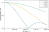 |
Fig. 2 Polarisation ratio (Lobs/Lint) of the linear polarisation as a function of RM for a frequency channel of width ∼0.976 MHz at three reference frequencies ν of 4, 5 and 6 GHz shown in blue, orange and green, respectively. Lobs is the observed linear polarisation and Lint is the intrinsic linear polarisation of the signal. The polarisation ratio is computed following Schnitzeler & Lee (2015) and starts to show significant depolarisation across our channel bandwidth at 4 GHz with RM ≳500 000 rad m−2. The RM polarisation ratio curve is symmetric around RM zero. |
3.1 Search in total intensity
We used PULSARX (Men et al. 2023) to dedisperse the total intensity data (Stokes I) in the DM range from 0 to 5000 pc cm−3 with DM steps of 2 pc cm−3 while simultaneously applying the zero-DM and Kadane filters (Eatough et al. 2009; Men et al. 2023) for further RFI cleaning. The search for periodicities in the dedispersed time series is performed in the Fourier domain with PRESTO (Ransom et al. 2002) in two passes: the first “low acceleration” pass allowing a frequency drift caused by a constant acceleration of up to 50 Fourier bins with up to 16 harmonics summed. The second pass is tuned to be more sensitive to non-linearly accelerated signals with up to 200 and 600 Fourier bins for the frequency drift and its derivative (the “jerk” search, Andersen & Ransom 2018), respectively. Due to limits in computing resources, we restricted the summation to 8 harmonics in the acceleration plus jerk search pass. Candidates for each pass are sifted separately to remove harmonically linked candidates or candidates with non-contiguous DM detections (see for more details Lazarus et al. 2015).
The folding of the remaining candidates is also done with PULSARX after we implemented the handling of full Stokes data and folding with “jerk” information. For each folded candidate with a measured pulse window, we could then apply within PULSARX the Faraday rotation measure (RM) synthesis method (Brentjens & de Bruyn 2005) to the detected pulse in the RM-range from −100 000 to +100 000 rad m−2 with steps of 5 units of RM. Beyond this range, the intra-channel depolarisation in the lowest part of our frequency band becomes detrimental (see Fig. 2). The RM synthesis plot along with the RM value that maximise the amount of linear polarisation are added to the traditional PULSARX inspection plot of each candidate. Due to memory limits in the computing nodes, we restricted the folding of the candidates with PULSARX to the first 210 candidates, sorted by PRESTO’s “sigma” values, the significance of each candidate in the Fourier domain for both the low acceleration and the acceleration plus jerk search pass. All candidates produced were visually inspected.
In addition to the periodicity search, we performed a search for single pulses on all pointings with TRANSIENTX (Men & Barr 2024) with the same RFI cleaning and dedispersion parameters as described above. Similar to our periodicity search, we modified TRANSIENTX such that it could handle our full Stokes search data and perform RM synthesis on the detected single pulse candidate. We recorded all events with a S/N greater than 6 for visual inspection.
3.2 Search for slow transients in linear polarization
Single-dish observations of the GC typically show a large amount of power fluctuations seen as red noise in the total intensity of the recorded time series due to, e.g. variations in atmospheric conditions and observed GC continuum emission (Eatough et al. 2021; Torne et al. 2021). This justified our choice of using the zero-DM technique in the total intensity search described in the previous section, but, in turn, it decreases our sensitivity towards very wide pulses as the dispersion delay (Lorimer & Kramer 2004) is limited to <1 s across our frequency band with our maximum DM trial.
In the light of the recent discoveries of slow and highly linearly polarised transients with periods greater than tens of seconds (e.g. Caleb et al. 2022; Hurley-Walker et al. 2022), we investigated a different approach to search for these very wide pulses in our data. First, the PSRFITS data were time-scrunched by a factor of 128 after the polarisation calibration step, resulting in a new time resolution of ∼16.7 ms. This allows us to limit the width of the boxcar used during the matched filtering process (Cordes & McLaughlin 2003) and drastically reduce the total number and length of time-series to be searched, making it more tractable with our current computing resources. Then we dedispersed the Stokes data with DM steps of 200 pc cm−3 up to a maximum value of 5000 pc cm−3 and applied a Faraday correction in the RM-range from −500 000 to +500 000 rad m−2 with steps of 40 rad m−2 using the complex linear polarisation form,  , where λ is the observed wavelength and Q, U are the Stokes Q and U vectors. Then we performed the frequency summation of the magnitude of L that was written to disk in PRESTO format to be later searched with PRESTO’s SINGLE_PULSE_SEARCH.PY using boxcar width up to 300 bins and a minimum S/N detection threshold of 7. Liu et al. (2021) have argued that searching in linear polarisation with data recorded with a linear feed is still plagued with the red noise fluctuations as in the total intensity search. However, Faraday correction with large RM values, i.e. |RM| ≳ 10 000 rad m−2, depolarises the baseline fluctuations, thus making our search insensitive to these fluctuations. We therefore applied this minimum RM-threshold when producing the summary plot and restricted our search in linear polarisation to the inner pointing on Sgr A∗ where RM is expected to be the largest.
3.3 Testing the processing pipeline
The processing pipeline described above was first tested on an 1-hr long observation of PSR J1746–2850, recorded as part of the RM monitoring of the GC pulsars with Effelsberg (Abbate et al. 2023), with the same observing setup as the one used in this work. PSR J1746–2850 (Deneva et al. 2009) is located about 12 arcmin away from Sgr A∗, close to the Quintuplet cluster, within the Radio Arc Bubble (Simpson et al. 2007). It has a rotational period of 1.07 s, a DM of about 960 pc cm−3, an RM of −12 234 ± 181 rad m−2 (Abbate et al. 2023) and a pulse profile that is roughly 50% linearly polarised. We successfully redetected PSR J1746−2850 in our low acceleration search pipeline with a S/N of 16. The RM estimated from the detected pulse window is −12 190 rad m−2 (see Fig. 3 for the detection plot) consistent with the measurement reported by Abbate et al. (2023).
To test the pipeline for slow-transient search in linear polarisation, we injected into one of our calibrated PSRFITS data three simulated full-Stokes pulse profiles created with PSRCHIVE that are fully linearly polarised with an RM of 10 000 rad m−2. These simulated pulse profiles of Gaussian shape share the same DM of 1750 pc cm−3 but have widths at a 50% intensity level of 0.2, 1.5, and 3 s, respectively. The dedispersed Stokes I time series with and without zero-DM subtraction are shown in Fig. 4 along with the Faraday rotation corrected linear polarisation time series (Ld). We ran SINGLE_PULSE_SEARCH.PY on the three time series and found that only the Ld dataset successfully recovered all three injected pulses without any other spurious candidates with a S/N above 7. This demonstrates that polarised bursts with wide widths can be efficiently detected in our survey through the search in linear polarisation.
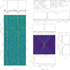 |
Fig. 3 Detection plot of the pulsar J1746−2850 produced by PulsarX. In addition to the panels described in Men et al. (2023), a new additional panel (a) shows the results of the RM synthesis analysis of the pulse delimited by the two vertical dashed lines of panel (b) for an evenly spaced grid of RM comprised between –50 000 rad m−2 and +50 000 rad m−2 with an RM step of 5 rad m−2. |
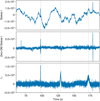 |
Fig. 4 Top panel: an excerpt of the total intensity (Stokes I) time series dedispersed at the DM of the injected pulses and exhibiting large amount of red noise. Middle panel: a view of the Stokes I time series dedispersed at the DM of the injected pulses and after subtraction of the zero DM time series. Bottom panel: time series of the linear polarisation Ld after dedispersion and the correction of Faraday rotation at RM = 10 000 rad m−2. For clarity, the average value of Ld has been subtracted from it. In all three panels, the grey dashed lines indicate the location of the three injected pulses. |
4 Results and discussion
4.1 Survey sensitivity
We compute the minimum mean flux density Smin of a pulsar with spin period Ps that can be detected by our survey with a significance σ using the modified radiometer equation from Cordes & Chernoff (1997),
 (1)
with Ssys = Tsys/G being the System Equivalent Flux Density (SEFD). Here β ≈ 1 is the degradation factor due to the 8-bit initial digitisation of the data, G = 1.5 K Jy−1 is the average gain of the Effelsberg telescope over our receiver bandwidth, and Tsys is the total system noise temperature. The number of summed polarisations np = 2, the chosen number of summed harmonics Nh, the effective bandwidth ∆f ∼ 3400 MHz after RFI cleaning, and the integration time Tint are parameters of the survey. The amplitude ratio in the Fourier domain of the h-th harmonic is
(1)
with Ssys = Tsys/G being the System Equivalent Flux Density (SEFD). Here β ≈ 1 is the degradation factor due to the 8-bit initial digitisation of the data, G = 1.5 K Jy−1 is the average gain of the Effelsberg telescope over our receiver bandwidth, and Tsys is the total system noise temperature. The number of summed polarisations np = 2, the chosen number of summed harmonics Nh, the effective bandwidth ∆f ∼ 3400 MHz after RFI cleaning, and the integration time Tint are parameters of the survey. The amplitude ratio in the Fourier domain of the h-th harmonic is  , see also e.g. Torne et al. (2023) for more details. The duty cycle of a pulsar’s averaged pulse, denoted ϵ = Weff/Ps with Weff being the effective pulse width, is affected by the sampling time, the intra-channel dispersion and temporal scattering that broadens the intrinsic pulse width Wi such that
 (2)
(2)
κ = 4.1488 × 10³ MHz2 pc−1 cm3 s is known as the dispersion constant, δf ≃ 0.97 MHz is the width of a single frequency channel, τ1GHz is the scattering timescale at a reference frequency ν of 1 GHz. For the inner pointing centred on the GC magnetar, we took τ1GHz = 1.3 s (Spitler et al. 2014). For all other pointings and without prior information, we assumed τ1GHz = 0.5 s. In all cases, the scattering index is α = −3.8 (Spitler et al. 2014).
As reported previously by e.g. Johnston et al. (2006) and Eatough et al. (2021), thermal and non-thermal emission from the GC dominate the contribution to Tsys at frequencies ≲8 GHz. Tsys also includes elevation-dependent contribution from spillover radiation from the ground (see measurements in Eatough et al. 2021). Continuum maps of the GC region (see e.g. Seiradakis et al. 1989; Reich et al. 1990; Law et al. 2008) shows that the continuum emission from the GC at a frequency of 5 GHz can reach up to a few hundreds of Jy at the position of Sgr A∗ and extend several arcmin away from the position of Sgr A∗ with a contribution of a few tens of Jy. This contradicts the assumption used in Suresh et al. (2022) to neglect the GC background contribution in the sensitivity calculations of their outer pointings.
To properly account for the GC contribution to our survey sensitivity, we used the individual pulsed noise diode observations fired at the sky position of each pointing and our observations of NGC 7027 to derive the SEFD for all pointings. SEFD measurements from inner to outer pointings are shown in Fig. 5 as well as with the SEFD measured at the sky location of PSR J1746−2850. We found an average SEFD value of 112 Jy (equivalent to Tsys = 168 K) for the inner pointing that encompasses Sgr A∗ and the GC magnetar J1745−2900. This result is consistent with the results from Eatough et al. (2021) when averaging their measurements at 4.85 GHz and 8.35 GHz. For the three outer rings, from inner to outer rings, we measured an SEFD average value of 87, 72, and 68 Jy, respectively. In addition, we measured an average SEFD value towards PSR J1746−2850 similar to the value for the outermost ring. This is again consistent with the continuum map from Law et al. (2008) as PSR J1746−2850 is located towards the Radio Arc.
Assuming a σ detection threshold of 8 and an intrinsic pulse duty cycle ϵi = Wi/Ps of 5%, we can derive our sensitivity limits in terms of pulsar luminosity and plot these curves as a function of spin period Ps in Fig. 6. For pulsars with Ps ≳ 50 ms, we obtain sensitivity limits between 2.8 and 1.7 mJy kpc2, from the inner pointing on Sgr A∗ towards the outer ring. Below these spin period, scattering effects degrade our survey sensitivity. These limits are significantly higher than the values reported in the GC survey by Suresh et al. (2022) done at a similar frequency with luminosity of 0.9 and 0.5 mJy kpc2, for the inner pointing on Sgr A∗ and all other pointings, respectively. However, we note here that Suresh et al. (2022) did neglect the GC continuum contribution to all off-Sgr A∗ pointings and used a continuum emission model (Rajwade et al. 2017) derived from maps produced by Law et al. (2008).
Now, we can estimate the fraction of the known Galactic pulsar population with a reported flux at 1.4 GHz (2350 pulsars in the ATNF Pulsar Catalog v 2.6.22 including 270 pulsars with Ps ≲ 30 ms) that would be detected by our survey, if placed at the distance of the GC. Following Jankowski et al. (2018), we drew, for each of the 2350 pulsars, a spectral index drawn from a normal distribution of mean –1.6 with standard deviation of 0.54 to derive the pulsar flux at 6 GHz. We find that not even the currently known most luminous MSPs would be detected if located in the inner pointing on Sgr A∗ while just some of the brightest MSPs could be detected in the outer pointings. Regarding the normal pulsar population (defined as Ps > 30 ms), up to 30% of this population could be detected by our survey assuming the best hypothesis (i.e. a pulsar located on-axis of the outer beam). This percentage decreases to 10% if we assume the sensitivity of a pulsar located on the edge of the inner beam. It could decrease even further as red noise in the data has been shown to reduce a survey’s sensitivity towards long period pulsars (Lazarus et al. 2015). We note here that our observing grid has been tightly packed assuming the HPBW at our highest observing frequency of 8 GHz, guaranteeing a more uniform sensitivity compared to past surveys.
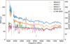 |
Fig. 5 Measured SEFD and Tsys as a function of observing frequency for a set of 4 survey pointings, from inner to outer rings (see Fig. 1). For comparison, we also added the SEFD measured at the sky location of PSR J1746–2850. The discontinuities in the SEFD curves are due to zapped frequency channels. |
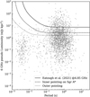 |
Fig. 6 Sensitivity curves of our GC survey as a function of pulsar spin period. The dashed and dotted lines indicate our sensitivity limits for the inner and most outer pointings of our grid with the grey points representing the inferred pseudo-luminosity of a galactic pulsar population at 6 GHz. For comparison, we added the well estimated sensitivity limit (the plain line) derived from the Sgr A∗ survey at 4.85 GHz by Eatough et al. (2021). |
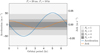 |
Fig. 7 Acceleration (blue line) and jerk (orange line) as a function of time for a binary pulsar of spin period 20 ms in a 6.7-h circular orbit around another neutron star of mass 1.35 M⊙. This simulation assumes an inclination angle of 60 degrees. The intersection of the grey bands indicate the sections of the orbit where our PRESTO acceleration and jerk search remains sensitive to the pulsar signal with the specified number of harmonics Nh. |
4.2 Sensitivity to orbital motion
The PRESTO binary pulsar search routine ACCELSEARCH performs matched filtering to remove Doppler induced frequency drifts in the Fourier detection spectrum. Following Ransom (2001) and Andersen & Ransom (2018), the frequency drift (expressed in Fourier bins) of pulsars under a constant acceleration, and constant jerk, are given by  and
and  respectively. Here f = 1/Ps is the spin frequency (or chosen harmonic of the spin frequency), a is the line of sight (l.o.s.) acceleration, j is the l.o.s jerk and c is the speed of light. Eatough et al. (2021), Liu et al. (2021), and Suresh et al. (2022) already discussed in detail the impact of orbital motion on the search sensitivity for pulsars orbiting Sgr A∗. Here our discussion primarily concerns the sensitivity to compact binary systems, although following Section 4.2 of Eatough et al. (2021) and given our maximum z-value of zmax = 200 bins, we expect to maintain a high degree of sensitivity to spin frequencies up to 1000 Hz from pulsars with circular orbital periods, Pb ≳ 120 d around Sgr A∗ in the central pointing.
Constant acceleration searches are sensitive to binaries where Tobs ≲ 0.1Pb, and acceleration plus jerk searches where Tobs ∼ 0.05Pb − 0.15Pb (Ransom 2001; Andersen & Ransom 2018). Therefore, with observations of Tint = 1 h it is expected that our survey remains sensitive to minimum orbital periods of Pb ∼ 6.7 h with our acceleration plus jerk search. If we consider a pulsar with spin frequency of 50 Hz in orbit around a second neutron star, we want to establish here if our chosen search range in z and w is sufficient for this detection. Fig. 7 shows the fraction of the 6.7 h-long orbit where our search can recover the drifted signal of the pulsar up to the desired number of harmonics. We estimate that only 15 and 30% of the orbit give acceleration low-enough such that the signal can be recovered with up to 8 and 4 harmonics, respectively, potentially severely degrading our sensitivity towards this tight binary. Our w-range is enough to cover the full orbit for frequencies up to the 4-th harmonic of the pulsar spin period.
Considering now a wider Pb ∼ 10 h orbit (see Fig. 8), the frequency drift due to acceleration can be recovered in 25%, 56%, 100% of the orbit with up to 8, 4 and 2 harmonics, respectively. In this case, the w-range is sufficient to recover the jerk through the full orbit up to the 8-th harmonic of the pulsar’s spin period.
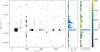 |
Fig. 9 Summary plot of the linear polarisation search. The left panel shows the RM of the single pulse candidates versus time with the size of the open circle marker indicating larger S/N (σ) with larger marker. The middle panel shows the number of single pulse detection per bin of RM. The panel on the right shows σ of the burst as function of its RM with a color scale corresponding to the detection DM. For clarity, the RM-range (y-axis) shown on all panels is restricted to −250 000; +250 000 rad m−2. As described in Section 3.2, candidates with |RM| <10 000 rad m−2 are excised. The detection of several bright pulses at DM of 1800 pc cm−3 and peaking at RM=−66 000 rad m−2 correspond to single pulses emitted by the SGR J1745−2900. |
4.3 Outcome of the survey
We visually inspected all periodicity candidates produced by PULSARX and found no new pulsar to date. The GC magnetar SGR J1745−2900 was not detected in the periodicity search of the inner pointing with the data recorded on March 2nd, 2020. The TRANSIENTX search for single pulses produced a set of about 2500 candidates and inspection plots from the 37 pointings. Among these candidates, about a tenth were attributed to the GC magnetar SGR 1745−2900, with 90% of them coming from the inner pointing. No promising candidate single pulse has been found with S/N above 8 and we report here on one tentative detection of a narrow pulse at DM = 4550 pc cm−2 with a S/N above 7 (see Fig. A.1).
After excluding several two-seconds time windows with ∼ 5 min periodicity that showed a large number of events with wide ranging RMs, the slow transient search in linear polarisation resulted in a set of 1033 pulses with S/N > 7 as reported by SINGLE_PULSE_SEARCH.PY (Fig. 9). The spurious candidates were attributed to a weather radar emitting polarised radio waves around 5.6 GHz in Germany. All the bright (i.e. with S/N > 10) SPs are clustered around DM = 1800 pc cm−3 and RM= −64 000 rad m−2 and most likely originate from the magnetar SGR J1745−2900. No other promising candidate was found.
5 Conclusions
We conducted between 2019 and 2020 a survey for pulsars and transients within the 10 pc region centred around Sgr A∗ at a central frequency of 6 GHz with the Effelsberg radio telescope.
The survey’s sensitivity was maximised by building a compact observing grid of 37 pointings around the sky location of SGR J1745−2900. We analysed the calibrated full-Stokes data with acceleration plus jerk search techniques such that our survey remained sensitive to non-fully recycled MSPs (i.e. with Ps ∼ 20 ms) in a putative 10-hr long circular orbit. The polarisation information provided another scoring input in the manually inspected diagnostic plots of pulsar and single pulse candidates produced by PULSARX and TRANSIENTX, respectively. No new pulsar or transient pulsed emission have been detected so far.
For the inner pointing encompassing Sgr A∗, we performed an additional search for slow transient emission in linear polarisation corrected for Faraday rotation. This analysis was justified by the presence of strong red noise in the data inherent to the nature of our single dish observations of the GC and it is shown to dramatically reduce the number of false alarm events in the single pulse diagnostic plot. However, this analysis only redetected the bright single pulse emission of the magnetar SGR J1745−2900.
A careful estimate of our survey sensitivity shows that, although it is a factor of three more sensitive than the limit presented by Eatough et al. (2021), it is still not sensitive to a population of MSPs in the vicinity of Sgr A∗ and hampered by the strong GC background emission. We also demonstrated that previous sensitivity limits for pulsar searches in the wider GC region were greatly overestimated and that the background noise contribution must be properly assessed as previously reported in Eatough et al. (2021). Yet, radio interferometers such as MeerKAT (Padmanabh et al. 2023) or the ngVLA (Bower et al. 2018) have the ability to resolve the background emission (see e.g. Hankins 1999; Kudale & Chengalur 2017) from the Sgr A∗ complex, and to allow for the subtraction of the incoherent beam and thus show exciting prospects for future GC pulsar surveys.
Acknowledgements
Based on observations with the 100-m telescope of the Max-Planck-Institut für Radioastronomie at Effelsberg. We acknowledge the use of the HPC systems Hercules and Raven at the Max Planck Computing and Data Facility where all computations were performed. The authors gratefully acknowledge support from the European Research Council (ERC) Synergy Grant “Black-HoleCam” Grant Agreement Number 610058. R.P.E. is supported by the Chinese Academy of Sciences President’s International Fellowship Initiative, grant No. 2021FSM0004. LS was supported by the National SKA Program of China (2020SKA0120100) and the Max Planck Partner Group Program funded by the Max Planck Society.
References
- Abbate, F., Noutsos, A., Desvignes, G., et al. 2023, MNRAS, 524, [Google Scholar]
- Andersen, B. C., & Ransom, S. M. 2018, ApJ, 863, L13 [Google Scholar]
- Bower, G. C., Chatterjee, S., Cordes, J., et al. 2018, in Astronomical Society of the Pacific Conference Series, 517, Science with a Next Generation Very Large Array, ed. E. Murphy, 793 [NASA ADS] [Google Scholar]
- Brentjens, M. A., & de Bruyn, A. G. 2005, A&A, 441, 1217 [NASA ADS] [CrossRef] [EDP Sciences] [Google Scholar]
- Caleb, M., Heywood, I., Rajwade, K., et al. 2022, Nat. Astron., 6, 828 [NASA ADS] [CrossRef] [Google Scholar]
- Cordes, J. M., & Chernoff, D. F. 1997, ApJ, 482, 971 [Google Scholar]
- Cordes, J. M., & Lazio, T. J. W. 2002, arXiv e-prints [arXiv:astro-ph/0207156] [Google Scholar]
- Cordes, J. M., & McLaughlin, M. A. 2003, ApJ, 596, 1142 [NASA ADS] [CrossRef] [Google Scholar]
- Deneva, J. S., Cordes, J. M., & Lazio, T. J. W. 2009, ApJ, 702, L177 [Google Scholar]
- Dexter, J., & O’Leary, R. M. 2014, ApJ, 783, L7 [Google Scholar]
- Eatough, R. P., Keane, E. F., & Lyne, A. G. 2009, MNRAS, 395, 410 [Google Scholar]
- Eatough, R. P., Falcke, H., Karuppusamy, R., et al. 2013, Nature, 501, 391 [Google Scholar]
- Eatough, R. P., Torne, P., Desvignes, G., et al. 2021, MNRAS, 507, 5053 [NASA ADS] [CrossRef] [Google Scholar]
- Faucher-Giguère, C.-A., & Loeb, A. 2011, MNRAS, 415, 3951 [Google Scholar]
- GRAVITY Collaboration (Abuter, R., et al.) 2020, A&A, 636, L5 [NASA ADS] [CrossRef] [EDP Sciences] [Google Scholar]
- Hankins, T. H. 1999, in Astronomical Society of the Pacific Conference Series, 180, Synthesis Imaging in Radio Astronomy II, eds. G. B. Taylor, C. L. Carilli, & R. A. Perley, 613 [Google Scholar]
- Heywood, I., Rammala, I., Camilo, F., et al. 2022, ApJ, 925, 165 [NASA ADS] [CrossRef] [Google Scholar]
- Hu, Z., & Shao, L. 2024, Phys. Rev. Lett., 133, 231402 [Google Scholar]
- Hurley-Walker, N., Zhang, X., Bahramian, A., et al. 2022, Nature, 601, 526 [NASA ADS] [CrossRef] [Google Scholar]
- Jankowski, F., van Straten, W., Keane, E. F., et al. 2018, MNRAS, 473, 4436 [Google Scholar]
- Johnston, S., Kramer, M., Lorimer, D. R., et al. 2006, MNRAS, 373, L6 [Google Scholar]
- Kaspi, V. M., & Beloborodov, A. M. 2017, ARA&A, 55, 261 [Google Scholar]
- Kennea, J. A., Burrows, D. N., Kouveliotou, C., et al. 2013, ApJ, 770, L24 [Google Scholar]
- Klein, B. 2005, PhD thesis, Rheinische Friedrich Wilhelms University of Bonn, Germany [Google Scholar]
- Kramer, M., Klein, B., Lorimer, D., et al. 2000, in Astronomical Society of the Pacific Conference Series, 202, IAU Colloq. 177: Pulsar Astronomy – 2000 and Beyond, eds. M. Kramer, N. Wex, & R. Wielebinski, 37 [Google Scholar]
- Kudale, S., & Chengalur, J. N. 2017, Exp. Astron., 44, 97 [Google Scholar]
- Law, C. J., Yusef-Zadeh, F., Cotton, W. D., & Maddalena, R. J. 2008, ApJSS, 177, 255 [Google Scholar]
- Lazarus, P., Brazier, A., Hessels, J. W. T., et al. 2015, ApJ, 812, 81 [NASA ADS] [CrossRef] [Google Scholar]
- Liu, K., Wex, N., Kramer, M., Cordes, J. M., & Lazio, T. J. W. 2012, ApJ, 747, 1 [Google Scholar]
- Liu, K., Desvignes, G., Eatough, R. P., et al. 2021, ApJ, 914, 30 [NASA ADS] [CrossRef] [Google Scholar]
- Lorimer, D. R., & Kramer, M. 2004, Handbook of Pulsar Astronomy, CUP, eds. R. Ellis, J. Huchra, S. Kahn, G. Rieke, & P. B. Stetson [Google Scholar]
- Macquart, J. P., Kanekar, N., Frail, D. A., & Ransom, S. M. 2010, ApJ, 715, 939 [Google Scholar]
- Men, Y., & Barr, E. 2024, A&A, 683, A183 [NASA ADS] [CrossRef] [EDP Sciences] [Google Scholar]
- Men, Y., Barr, E., Clark, C. J., Carli, E., & Desvignes, G. 2023, A&A, 679, A20 [NASA ADS] [CrossRef] [EDP Sciences] [Google Scholar]
- Padmanabh, P. V., Barr, E. D., Sridhar, S. S., et al. 2023, MNRAS, 524, 1291 [NASA ADS] [CrossRef] [Google Scholar]
- Psaltis, D., Wex, N., & Kramer, M. 2016, ApJ, 818, 121 [Google Scholar]
- Rajwade, K. M., Lorimer, D. R., & Anderson, L. D. 2017, MNRAS, 471, 730 [Google Scholar]
- Ransom, S. M. 2001, PhD thesis, Harvard University, Massachusetts, USA Ransom, S. M., Eikenberry, S. S., & Middleditch, J. 2002, AJ, 124, 1788 [Google Scholar]
- Rea, N., Esposito, P., Pons, J. A., et al. 2013, ApJ, 775, L34 [Google Scholar]
- Reich, W., Fürst, E., Reich, P., & Reif, K. 1990, A&AS, 85, 633 [Google Scholar]
- Schnitzeler, D. H. F. M., & Lee, K. J. 2015, MNRAS, 447, L26 [Google Scholar]
- Seiradakis, J. H., Reich, W., Wielebinski, R., Lasenby, A. N., & Yusef-Zadeh, F. 1989, A&AS, 81, 291 [Google Scholar]
- Simpson, J. P., Colgan, S. W. J., Cotera, A. S., et al. 2007, ApJ, 670, 1115 [Google Scholar]
- Spitler, L. G., Lee, K. J., Eatough, R. P., et al. 2014, ApJ, 780, L3 [Google Scholar]
- Suresh, A., Cordes, J. M., Chatterjee, S., et al. 2022, ApJ, 933, 121 [NASA ADS] [CrossRef] [Google Scholar]
- Torne, P., Desvignes, G., Eatough, R. P., et al. 2021, A&A, 650, A95 [NASA ADS] [CrossRef] [EDP Sciences] [Google Scholar]
- Torne, P., Liu, K., Eatough, R. P., et al. 2023, ApJ, 959, 14 [NASA ADS] [CrossRef] [Google Scholar]
- van Straten, W., Demorest, P., & Oslowski, S. 2012, Astron. Res. Technol., 9, 237 [NASA ADS] [Google Scholar]
- Wharton, R. S. 2017, PhD thesis, Cornell University, New York, USA [Google Scholar]
- Wharton, R. S., Chatterjee, S., Cordes, J. M., Deneva, J. S., & Lazio, T. J. W. 2012, ApJ, 753, 108 [Google Scholar]
- Zhao, J.-H., Morris, M. R., & Goss, W. M. 2016, ApJ, 817, 171 [NASA ADS] [CrossRef] [Google Scholar]
Appendix A Inspection plot
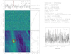 |
Fig. A.1 Single pulse candidate produced by TransientX, see Men & Barr (2024) for a description of the panels. Faraday synthesis is applied to the detected pulse window with the result shown in the bottom-right panel. No significant peak in the RM spectrum is detected. |
All Figures
|
Fig. 1 Left panel: image of the GC region produced by MeerKAT at 1.28 GHz (Heywood et al. 2022) with the positions of the known pulsars indicated by blue crosses (or a blue arrow in the case of the recently discovered millisecond pulsar J1744−2946, 9′ away from the edge of the map). The region delineated by the square box marked with the letter A is displayed in the right hand panel. The dashed grey circle delimits the 10 pc region around Sgr A∗ at the distance of the GC. Right panel: observing grid superimposed on a radio map of the GC obtained at 5.5 GHz with the Very Large Array (Zhao et al. 2016). Each coloured circle with the pointing number at its center represents the beam size at HPBW at 8 GHz θ8GHz = 1.55′ with the color corresponding to the pointing System Equivalent Flux Density (SEFD) value shown with the vertical colour bar. The blue cross at the center of the dotted circle indicate the location of the magnetar SGR J1745−2900. For clarity, we omit the numerical label of the inner pointing centred on Sgr A∗. The dotted grey circle delimits the 10 pc region around Sgr A*. |
| In the text | |
|
Fig. 2 Polarisation ratio (Lobs/Lint) of the linear polarisation as a function of RM for a frequency channel of width ∼0.976 MHz at three reference frequencies ν of 4, 5 and 6 GHz shown in blue, orange and green, respectively. Lobs is the observed linear polarisation and Lint is the intrinsic linear polarisation of the signal. The polarisation ratio is computed following Schnitzeler & Lee (2015) and starts to show significant depolarisation across our channel bandwidth at 4 GHz with RM ≳500 000 rad m−2. The RM polarisation ratio curve is symmetric around RM zero. |
| In the text | |
|
Fig. 3 Detection plot of the pulsar J1746−2850 produced by PulsarX. In addition to the panels described in Men et al. (2023), a new additional panel (a) shows the results of the RM synthesis analysis of the pulse delimited by the two vertical dashed lines of panel (b) for an evenly spaced grid of RM comprised between –50 000 rad m−2 and +50 000 rad m−2 with an RM step of 5 rad m−2. |
| In the text | |
|
Fig. 4 Top panel: an excerpt of the total intensity (Stokes I) time series dedispersed at the DM of the injected pulses and exhibiting large amount of red noise. Middle panel: a view of the Stokes I time series dedispersed at the DM of the injected pulses and after subtraction of the zero DM time series. Bottom panel: time series of the linear polarisation Ld after dedispersion and the correction of Faraday rotation at RM = 10 000 rad m−2. For clarity, the average value of Ld has been subtracted from it. In all three panels, the grey dashed lines indicate the location of the three injected pulses. |
| In the text | |
|
Fig. 5 Measured SEFD and Tsys as a function of observing frequency for a set of 4 survey pointings, from inner to outer rings (see Fig. 1). For comparison, we also added the SEFD measured at the sky location of PSR J1746–2850. The discontinuities in the SEFD curves are due to zapped frequency channels. |
| In the text | |
|
Fig. 6 Sensitivity curves of our GC survey as a function of pulsar spin period. The dashed and dotted lines indicate our sensitivity limits for the inner and most outer pointings of our grid with the grey points representing the inferred pseudo-luminosity of a galactic pulsar population at 6 GHz. For comparison, we added the well estimated sensitivity limit (the plain line) derived from the Sgr A∗ survey at 4.85 GHz by Eatough et al. (2021). |
| In the text | |
|
Fig. 7 Acceleration (blue line) and jerk (orange line) as a function of time for a binary pulsar of spin period 20 ms in a 6.7-h circular orbit around another neutron star of mass 1.35 M⊙. This simulation assumes an inclination angle of 60 degrees. The intersection of the grey bands indicate the sections of the orbit where our PRESTO acceleration and jerk search remains sensitive to the pulsar signal with the specified number of harmonics Nh. |
| In the text | |
 |
Fig. 8 Same as Fig. 7 but assuming a 10-h circular orbit. |
| In the text | |
|
Fig. 9 Summary plot of the linear polarisation search. The left panel shows the RM of the single pulse candidates versus time with the size of the open circle marker indicating larger S/N (σ) with larger marker. The middle panel shows the number of single pulse detection per bin of RM. The panel on the right shows σ of the burst as function of its RM with a color scale corresponding to the detection DM. For clarity, the RM-range (y-axis) shown on all panels is restricted to −250 000; +250 000 rad m−2. As described in Section 3.2, candidates with |RM| <10 000 rad m−2 are excised. The detection of several bright pulses at DM of 1800 pc cm−3 and peaking at RM=−66 000 rad m−2 correspond to single pulses emitted by the SGR J1745−2900. |
| In the text | |
|
Fig. A.1 Single pulse candidate produced by TransientX, see Men & Barr (2024) for a description of the panels. Faraday synthesis is applied to the detected pulse window with the result shown in the bottom-right panel. No significant peak in the RM spectrum is detected. |
| In the text | |
Current usage metrics show cumulative count of Article Views (full-text article views including HTML views, PDF and ePub downloads, according to the available data) and Abstracts Views on Vision4Press platform.
Data correspond to usage on the plateform after 2015. The current usage metrics is available 48-96 hours after online publication and is updated daily on week days.
Initial download of the metrics may take a while.