| Issue |
A&A
Volume 706, February 2026
|
|
|---|---|---|
| Article Number | A134 | |
| Number of page(s) | 9 | |
| Section | Stellar structure and evolution | |
| DOI | https://doi.org/10.1051/0004-6361/202556462 | |
| Published online | 05 February 2026 | |
Studying the surface effect in Procyon A as an F-type star
INAF-IAPS Via del Fosso del Cavaliere 100 00133 Roma, Italy
★ Corresponding author: This email address is being protected from spambots. You need JavaScript enabled to view it.
Received:
17
July
2025
Accepted:
26
December
2025
Abstract
Context. Procyon A is an F-type main-sequence star in a binary system. It has been the subject of numerous ground-based and space-based observing campaigns, providing precise classical constraints, including a well-determined mass. It was also among the first stars in which individual frequencies were detected, making it a crucial benchmark for F-type stars.
Aims. Our goal is to investigate the surface effect, namely the discrepancy between observed and model oscillation frequencies due to inadequate modeling of the surface stellar layers, which is especially important in F-type stars. Using Procyon A as a case study, we aim to understand how different surface correction prescriptions impact the inference of the fundamental properties of this star, and to compare the results with those obtained when the surface corrections are neglected.
Methods. We inferred the fundamental stellar properties by employing a grid of models computed with Modules for Experiments in Stellar Astrophysics (MESA), including gravitational settling, radiative accelerations, and turbulent mixing. We selected the best-fit models using the Asteroseismic Inference on a Massive Scale (AIMS) code, taking into account different methods to fit the individual frequencies.
Results. We find that the use of surface corrections can introduce uncertainties of up to 7% in the inferred stellar mass. We obtain the most reliable stellar mass estimates when using frequency ratios, the Sonoi surface correction, or direct fitting of the individual frequencies.
Conclusions. Our results indicate that the surface effects in F-type stars differ from those found in the Sun and in solar-like stars, highlighting the need for caution when considering the surface corrections for these stars.
Key words: asteroseismology / stars: evolution / stars: individual: Procyon A
© The Authors 2026
 Open Access article, published by EDP Sciences, under the terms of the Creative Commons Attribution License (https://creativecommons.org/licenses/by/4.0), which permits unrestricted use, distribution, and reproduction in any medium, provided the original work is properly cited.
This article is published in open access under the Subscribe to Open model. This email address is being protected from spambots. You need JavaScript enabled to view it. to support open access publication.
1. Introduction
Procyon is a binary star system consisting of an F-type main-sequence primary and a white dwarf secondary component. Procyon A has been the focus of various studies because it is the first star, other than the Sun, in which solar-like oscillations were clearly detected (Brown et al. 1991).
Early attempts to resolve the seismic frequencies yielded unsatisfactory results. Ground-based observations by Martić et al. (1999) succeeded in detecting the presence of oscillations, but were unable to resolve the individual modes. Subsequently, Eggenberger et al. (2004) confirmed oscillations and identified a few individual mode frequencies. Attempts to confirm the individual frequencies using space photometry were carried out with the Canadian Microvariability and Oscillations of STars satellite (MOST; Walker et al. 2003); however, because of suboptimal noise levels and lower-than-expected oscillation amplitudes, it was not possible to resolve any excess power (Bedding et al. 2005). More recently, Bedding et al. (2010) analyzed a combined series of data collected from high-precision, ground-based observations and successfully identified more than fifty individual oscillation frequencies. This accurate set of oscillation frequencies can be combined with precise determinations of the radius and luminosity from interferometry and parallax, as measured by the Very Large Telescope Interferometer (Aufdenberg et al. 2005) and Gaia DR3 (Soubiran et al. 2024), together with spectroscopic determination of metallicity and effective temperature from the High Accuracy Radial Velocity Planet Searcher (HARPS; Perdelwitz et al. 2024). Furthermore, since Procyon is a binary system, the masses of both components are tightly constrained (Girard et al. 2000; Gatewood & Han 2006; Bond et al. 2015). Due to this wealth of high-quality data, Procyon has become a unique testing ground for stellar models (e.g., Eggenberger et al. 2005; Straka et al. 2005; Guenther et al. 2014).
F-type stars are particularly challenging to study due to their distinct stellar structure, characterized by a convective core during the main sequence (MS) and a very thin convective envelope. A major difficulty lies in the detection of solar-like oscillations, as their high effective temperatures lead to shorter mode lifetimes and broader line widths, which render the oscillation modes unresolved and difficult to distinguish (White et al. 2012).
Only a limited number of F-type stars exhibit detectable individual oscillation mode frequencies. HD 49933, an F-type star similar to Procyon A, exhibits solar-like oscillations detected by the onvection, Rotation and planetary Transits mission (CoRoT; Michel et al. 2008). Along with Procyon, HD 49933 is among the most studied F-type stars and has been widely used as a laboratory for magnetic activity (e.g., Garcia et al. 2010; Ceillier et al. 2011). Other F-type stars showing high-quality individual frequencies include 22 stars in the Kepler LEGACY sample (Lund et al. 2017), which represents the best seismic detections obtained with the Kepler telescope (Borucki et al. 2010). These stars have been used in various studies to test stellar models and investigate different physical properties, such as determining the depth of the convective zone (e.g., Deal et al. 2023, 2025) and understanding the surface chemical evolution (e.g., Verma et al. 2019; Verma & Silva Aguirre 2019; Moedas et al. 2025). Nevertheless, Procyon A remains one of the few F-type stars with a dynamical mass determination. This provides an invaluable constraint that can be used to validate stellar models.
With the upcoming launch of the PLAnetary Transits and Oscillations of stars space mission (PLATO/ESA; Rauer et al. 2025), high-precision asteroseismic data will become available, providing mass, radius, and age determinations with expected uncertainties of 15%, 2%, and 10% for Sun-like stars, respectively. Achieving this level of precision requires accurate stellar models. However, current stellar models remain subject to significant uncertainty. Therefore, it is necessary to identify and quantify the inaccuracies in stellar models and to improve our modeling techniques. One of the current challenges in stellar modeling is the treatment of surface effects. A well-known systematic discrepancy exists between the observed and modeled frequencies of the Sun and solar-type stars (Christensen-Dalsgaard et al. 1988, 1996; Dziembowski et al. 1988; Christensen-Dalsgaard & Thompson 1997). This discrepancy arises from inadequacies in our modeling of the stellar surface layer. We still have an incomplete understanding of how to model the internal thermal gradient in the superadiabatic regions of stars. Currently, we use the adiabatic approximation to calculate the seismic frequencies. Additionally, we do not fully understand how to model convection and magnetic fields correctly in the surface layer. These issues are collectively referred to as surface effects. Several empirical formulas have been developed to correct for the discrepancies caused by these surface effects (see, for example, Kjeldsen et al. 2008; Ball & Gizon 2014; Sonoi et al. 2015). However, these surface corrections were developed for the Sun, and while they may be applicable to solar-type stars, their validity for stars with different effective temperatures may be limited, particularly in the case of F-type stars. These stars exhibit distinct stellar structures and possess remarkably thin convective envelopes, suggesting that the level and nature of surface effects may differ. Moreover, these corrections lack a direct physical interpretation. In this study, we focus on Procyon A because its stellar parameters, particularly its mass, are well constrained. We used Procyon A to examine how surface corrections perform in inferring the global stellar properties and to determine whether the corrections remain valid for an F-type star.
This article is structured as follows: in Sect. 2, we present the most recent observable parameters of Procyon A. In Sect. 3, we describe the optimization method and the models used. The test performed to select the frequency scenarios is presented in Sect 4. We present our results from testing the different surface corrections in Sect. 5 and summarize our conclusions in Sect. 6.
2. Observable parameters
Procyon is a well-known binary star system. Astrometric measurements allow the precise determination of the stellar masses of its two components. The most recent estimates, based on Hubble Space Telescope data, were provided by Bond et al. (2015), who derived masses of 1.478 ± 0.012 M⊙ for Procyon A and 0.592 ± 0.006 M⊙ for Procyon B. These values provide strict constraints for validating stellar evolution and asteroseismic models.
To constrain the primary component, Procyon A, we adopted the most recent spectroscopic and photometric measurements. The stellar luminosity (L = 7.049 ± 0.064 L⊙) and the radius (R = 2.046 ± 0.009 R⊙) were determined by Soubiran et al. (2024) using Gaia parallaxes and interferometric angular diameters Gaia Collaboration (2021). We adopted spectroscopic parameters such as effective temperature (Teff), surface gravity (log(g)), and iron content ([Fe/H]) from Perdelwitz et al. (2024), who report Teff = 6768.8 ± 70.0 K, log(g) = 4.056 ± 0.066 dex, and [Fe/H] = 0.00 ± 0.056 dex (see Table 1). Figure 1 shows the location of Procyon A in the Kiel diagram.
Fundamental parameters of Procyon A.
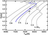 |
Fig. 1. Kiel diagram showing computed evolutionary tracks with metallicity [M/H]i = 0.0 and Yi = 0.26 (solar composition) as solid gray lines. The star symbol marks the location of Procyon A in the diagram. The solid blue line represents the evolutionary track of the best model (circle symbol) from the r02 test, considering the radius in the inference of scenario A. |
High-precision asteroseismic observations by Bedding et al. (2010) revealed a set of individual p-mode frequencies (νn, ℓ) with radial order n and harmonic degree ℓ in Procyon A, based on combined data from 11 telescopes (Arentoft et al. 2008). Two alternative mode identifications were proposed, referred to as scenario A and scenario B, each comprising approximately 50 modes of degree ℓ = 0, 1, and 2. Due to challenges in ridge identification in the échelle diagram (a plot in which oscillation frequencies are folded modulo the large frequency separation to reveal regular mode patterns), we considered both scenarios, focusing on the ℓ = 0 and ℓ = 1 modes. Observationally, Bedding et al. (2010) and White et al. (2012) found some evidence favoring scenario B. However, several modeling studies (Doğan et al. 2010; Guenther et al. 2014; Compton et al. 2019) have shown that only scenario A leads to acceptable stellar models that are consistent with the observed global and seismic parameters.
3. Stellar models and inference method
3.1. Stellar models
In this study, we used grid C of the stellar models developed by Moedas et al. (2025), which was computed using the MESA code (Paxton et al. 2011, 2013, 2015, 2018, 2019). This grid incorporates up-to-date stellar physics. In particular, it includes atomic diffusion and the effects of radiative acceleration, which are calculated using the single-valued parameter (SVP) method (LeBlanc & Alecian 2004; Alecian & LeBlanc 2020). To avoid unrealistic surface chemical variations caused by diffusion, the grid uses a turbulent mixing prescription calibrated by Verma & Silva Aguirre (2019) to reproduce the observed surface helium abundance in F-type stars.
The impact of using chemical transport mechanisms, such as radiative accelerations and turbulent mixing, to characterize F-type stars is investigated in Moedas et al. (2024, 2025). Using a sample of 91 FGK-type stars from Davies et al. (2016), Lund et al. (2017), the authors find that neglecting atomic diffusion in stellar models of F-type stars can introduce uncertainties of up to 10%, 4%, and 29% when inferring the stellar mass, radius, and age, respectively. Since this is outside the scope of our work, we did not investigate how chemical transport mechanisms affect modeling Procyon A; however, the results and conclusions should remain consistent when the same physical inputs are used in stellar models.
3.2. Optimization
For the inference of the stellar properties, we employed the AIMS code (Rendle et al. 2019), following the approach of Moedas et al. (2024, 2025). Here, we provide a brief overview of the optimization process. The AIMS code is a Bayesian optimization tool that uses Markov chain Monte Carlo (MCMC) methods to explore the parameter space of stellar-model grids and identify the model that best fits the observational constraints. The AIMS framework distinguishes between the contributions of the global constraints, Xi (in our case Teff, [Fe/H], and R),
 (1)
(1)
and the constraints from individual frequencies, νi,
 (2)
(2)
where “(obs)” corresponds to the observed values and “(mod)” corresponds to the calculated model values. The weight that AIMS assigns to the seismic contribution can be absolute (3:N), in which each individual frequency has the same weight as each global constraint,
 (3)
(3)
It is important to note that the χ2 values reported in this work (and provided by AIMS) are the raw sums of squared residuals, not divided by the number of degrees of freedom (reduced χ2). Therefore, they should be interpreted primarily as the objective function minimized by the Bayesian optimization engine to select the best-fit models, rather than as a standard goodness-of-fit statistic for strictly comparing models with different degrees of freedom.
To interpret the statistics, we can calculate a reduced χr2, defined as
 (4)
(4)
where N is the number of constraints in the calculation of χ2.
3.3. Data analysis
Because this study uses a single star to compare surface corrections, we cannot make strong statistical claims. However, since several stellar properties of Procyon A, such as its mass determined from interferometry, are well known, we can evaluate how accurately each surface prescription characterizes this star. To compare the inferred results with the observational parameters, we computed the relative difference, defined as
 (5)
(5)
where X represents a given stellar parameter, Xm is the value inferred from the model, and Xr is the reference observational value. This expression provides a measure of the discrepancy between the model prediction and the reference observed values. Additionally, we computed a normalized difference, defined as
 (6)
(6)
where σ(Xm) is the uncertainty of the inferred parameter. This quantity indicates how far the model result deviates from the expected values in units of the 1σ uncertainty. We caution, however, that z depends on the model-inferred uncertainties σ(Xm), which can vary significantly between different models and parameters, depending on the shape of the posterior distribution. Therefore, z is not a standard statistical metric and should not be used as a primary diagnostic for model selection. Instead, we used it as a qualitative indicator to easily visualize the agreement between the inferred and reference values.
3.4. Surface corrections
A well-known issue in asteroseismic modeling is the surface effect, which is a systematic discrepancy (δν) between observed and theoretical frequencies of individual stars that arises from simplified modeling of the near-surface stellar layers. Two main approaches are used to compare observations and models. The first involves applying empirical surface corrections to compensate for the offset between modeled and observed frequencies, while the second relies on comparing ratios of small to large frequency separations rather than the individual frequencies. Several surface-correction prescriptions exist; in this work, we investigate the three most commonly applied formulations.
The first correction we considered was developed by Kjeldsen et al. (2008, hereafter KJ08). Using the Sun as a reference, they found that the offset between the observed and model frequencies could be described by a power law:
 (7)
(7)
where a and b are the correction parameters and ν(max) is the maximum power frequency.
The second prescription was proposed by Ball & Gizon (2014, hereafter BG14). In their approach, the discrepancy was described by two terms that account for the mode inertia (I). The correction is described as
![Mathematical equation: $$ \begin{aligned} \delta \nu =\left[a_3\left(\frac{\nu _i}{\nu _\mathrm{ac} }\right)^3+a_{-1}\left(\frac{\nu _i}{\nu _\mathrm{ac} }\right)^{-1}\right]/I, \end{aligned} $$](/articles/aa/full_html/2026/02/aa56462-25/aa56462-25-eq8.gif) (8)
(8)
where a3 and a−1 are the correction parameters and νac is the acoustic cut-off frequency, which is the maximum frequency at which pressure modes can be reflected back into the stellar interior rather than escaping into the atmosphere. The first term describes the contribution of the magnetic field (∝νi3), and the second term accounts for the contribution of the convection (∝νi−1). As shown by BG14, the first term dominates the correction, allowing the second term to be neglected so that Eq. (8) can be simplified as
![Mathematical equation: $$ \begin{aligned} \delta \nu =\left[a_3\left(\frac{\nu _i}{\nu _\mathrm{ac} }\right)^3\right]/I. \end{aligned} $$](/articles/aa/full_html/2026/02/aa56462-25/aa56462-25-eq9.gif) (9)
(9)
Hereafter, we refer to the two-term correction (Eq. (8)) as BG142 and the one-term correction (Eq. (9)) as BG141.
The final prescription we investigated was proposed by Sonoi et al. (2015, hereafter SO15). According to SO15, previously formulated surface corrections depend strongly on the star’s Teff and log(g), because the structure of the stellar surface varies with these parameters. They also emphasize that the surface corrections should not be calibrated on the Sun, but should instead be constrained by model physics. Based on 3D models of stellar surface layers, SO15 proposed a modified Lorentzian function to describe the frequency offsets, given by
![Mathematical equation: $$ \begin{aligned} \frac{\delta \nu }{\nu _\mathrm{max} }=\alpha \left[1-\frac{1}{1-\left(\nu _\mathrm{(obs)} /\nu _\mathrm{max} \right)^\beta }\right], \end{aligned} $$](/articles/aa/full_html/2026/02/aa56462-25/aa56462-25-eq10.gif) (10)
(10)
where α and β are free parameters.
The second method for comparing stellar models with asteroseismic observations was introduced by Roxburgh & Vorontsov (2003) and is based on the ratio of the small to large frequency separations. The most commonly used small separation is calculated as the difference between two modes with consecutive radial order n but different ℓ:
 (11)
(11)
Here, νn, 0 is the frequency of the radial mode (ℓ = 0) of radial order n, and νn − 1, 2 is the frequency of the quadrupole mode (ℓ = 2) of radial order n − 1.
This quantity is particularly useful because it is sensitive to the structure of the stellar core. It is defined by the integral of the sound-speed gradient in the core, which depends on the composition gradients and is therefore directly related to the evolutionary stage of the star:
 (12)
(12)
where c(r) is the sound speed and r is the radius. The calculation of Eq. (11) requires the detection of modes with ℓ = 2, which are not always observable. Therefore, other small separations can be considered, such as d01 and d10, which are defined by the so-called five-point separations:
 (13)
(13)
Using the small separations, we can define the frequency ratios as
 (14)
(14)
where Δνℓ(n) is the large frequency separation, defined by the asymptotic relation (Tassoul 1980)
 (15)
(15)
For a more detailed description, we refer to Roxburgh & Vorontsov (2003). These ratios constitute a set of constraints that are more sensitive to the interior of the star and nearly independent of the structure of the outer layers. These ratios allow us to avoid surface corrections and compare models with observations more robustly. However, they require a sufficiently large set of individual frequencies and lose some information about the outer layers, making it more difficult to accurately infer the mean density of the observed star.
4. Scenario A versus scenario B
Our goal is to evaluate how different surface corrections perform in inferring stellar properties. However, we must adopt one of the frequency sets provided in Bedding et al. (2010). To avoid dependence on surface corrections, we tested both frequency scenarios using frequency ratios, which are independent of surface corrections and thus provide more robust constraints on the stellar interior. We performed three tests. In test 1, we used the three frequency ratios (r01, r10, and r02), and therefore all mode frequencies were included. In test 2, we used r02 and only modes with ℓ = 0 and ℓ = 2 were considered, excluding ℓ = 1 modes in the optimization process. This approach avoids issues arising from mixed modes or incorrect mode identification. In test 3 (rℓ, red), we neglected the frequencies above which a discontinuity in the solar-like asymptotic behavior occurs (Eq. (15)). To infer the stellar properties, we used the frequency ratios as seismic constraints. These constraints were computed from the individual mode frequencies corresponding to each scenario. For the classic constraints, we performed two tests: one considering Teff and [Fe/H] and another that included R as an additional constraint. For each test, we obtained four sets of inferred stellar properties: two for each scenario depending on whether R was included as a constraint. This setup allowed us to investigate the impact of including R on the results. Table 2 shows the results of each test, while the relative and normalized differences are reported in Table 3.
Inferred stellar properties from each test for the two frequency scenarios.
Relative and normalized differences of the inferred stellar properties for each test and for the two frequency scenarios.
Figure 2 shows the relative differences for test 1. When using all the frequency ratios, the model fails to reproduce the stellar properties accurately (except for log g), yielding unrealistic values for the stellar mass. Including the radius as an additional constraint in the fitting procedure does not improve the stellar inference, as all tests show a relative mass difference of approximately 17–18%. Only scenario B is able to recover the stellar radius, even without explicitly using it as a constraint. Moreover, the normalized differences indicate that none of the inferred parameters (except R in scenario B) fall within the expected observational uncertainties, either at the 1σ (z ≤ 1) or 3σ (z ≤ 3) level, with z defined in Eq. (6). Nevertheless, the χ2 values for both frequency sets are extremely large, suggesting poor convergence in the optimization process and indicating that the difference in frequencies is the main contributor to the χ2 estimate. This may point to an issue with the seismic constraints themselves. As noted by Bedding et al. (2010), the presence of a low-frequency mixed mode for ℓ = 1 could introduce inconsistencies during the optimization process.
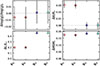 |
Fig. 2. Relative difference between the inferred and reference values (subscript r) obtained in test 1 for the two frequency sets (Scenarios A and B). The top-left panel shows the surface gravity, the top-right panel the surface radius, bottom-left panel the surface luminosity, and bottom-right panel the stellar mass. The dotted line indicates where the relative difference is zero. |
Figure 3 shows the results for test 2, where we observe significant improvements in the determination of the stellar parameters. For scenario A, the stellar mass of Procyon A is reproduced within 1σ uncertainties, with a relative difference of 4% when R is neglected and 1% when included in the optimization. Scenario B also shows an improvement, but the inferred stellar mass still deviates by approximately 10%. The χ2 values from the optimization show a substantial improvement compared to test 1. To illustrate the frequency fits, Figs. 5 and 6 show the r02 ratios and the échelle diagrams of the individual frequencies for the best-fit model. Both scenarios fit the ratios reasonably well, but in the échelle diagram, the high-frequency modes of Scenario A deviate slightly from the observations, as expected due to surface effects. In contrast, scenario B does not reflect the expected asymptotic behavior in the diagram, and the inferred frequencies cannot be explained by surface effects. Overall, scenario A reproduces the stellar parameters more accurately. It also matches the observed ridge pattern more accurately and provides a more reliable basis for inferring the stellar properties.
Before selecting the frequency set, we highlight the frequency glitch visible in Fig. 6, which appears at high frequencies in scenario A for ℓ = 1 and in scenario B for ℓ = 0 and 2. To assess its impact on the inference and any resulting bias toward scenario A, we performed test 3, excluding the affected high-frequency modes from the optimization. Figure 4 shows the resulting parameter differences. In this test, scenario B reproduces the stellar mass of Procyon A when the radius is included in the optimization process, whereas scenario A shows a slightly larger discrepancy and recovers the expected mass only within 2σ uncertainties. Nevertheless, scenario A yields a smaller χ2 and a smaller relative difference than scenario B. In the échelle diagram (bottom row of Fig. 6), scenario A performs worse than in test 2, but still follows the observed pattern more closely than scenario B, which does not show significant changes from the previous test. Compared to test 1, test 3 represents a significant improvement. This suggests that the optimization issue may arise from fitting the glitch at higher frequencies, likely due to missing physics in the stellar models, rather than in the possible mixed-mode at low frequencies for ℓ = 1.
Tests 2 and 3 indicated that scenario A best fits Procyon A, whereas White et al. (2012) favored scenario B. However, other modeling studies of Procyon A (Doğan et al. 2010; Guenther et al. 2014; Compton et al. 2019) reproduce its stellar mass adopting the frequencies of scenario A. We consider two possible explanations. The first is that inaccuracies in the stellar models are compensated for by scenario A. However, because previous studies Doğan et al. (2010), Guenther et al. (2014), Compton et al. (2019) and the present study use different input physics in the stellar models, and all favor scenario A, model inaccuracies alone are unlikely to explain the discrepancy. This supports the idea that Scenario A represents the correct frequency identification. The second possibility is a misidentification of the observed modes, which could render the inferences for scenario B inconsistent and those for scenario A more coherent. This issue remains under debate, and we hope that forthcoming observations from the Transiting Exoplanet Survey Satellite (TESS; Ricker 2016) will provide a definitive answer. Although White et al. (2012) found observational evidence that favors scenario B based on the identification of the ridge in the échelle diagram, our modeling results align with previous theoretical studies (e.g., Guenther et al. 2014) in favor of scenario A. While the statistical difference in terms of raw χ2 is moderate, scenario A consistently yields a dynamical mass in better agreement with the precise interferometric value (1.478 M⊙), particularly when the radius is included as a constraint. In contrast, scenario B often requires stellar parameters that deviate significantly from the spectroscopic or dynamical constraints to achieve a seismic fit. Therefore, we adopt scenario A as the seismic constraint for the remainder of this work. Although scenario A has the smaller χ2, the reduce value is similar to that of scenario B and is not statistically significant. Nevertheless, scenario A offers the most physically consistent agreement with the global observational parameters, showing smaller relative differences and reproducing the expected asymptotic behavior of the frequencies.
In the following sections, we adopt the result from test 2 including R as the reference, since it provides the best characterization of Procyon A. For the surface corrections tests, we exclude the ℓ = 1 modes from the optimizations and keep R as a constraint for consistency.
5. Testing surface corrections
In Sect. 4, our tests indicate that scenario A best reproduces Procyon A. Here, we examine how well the surface corrections under study reproduce the stellar properties of our star. Tables 4 and 5 present the stellar parameters obtained for each surface correction, along with their respective normalized differences from the observed values (Fig. 7).
Inferred properties for the different surface corrections.
Relative and normalized differences of stellar properties for tests of different surface-frequency corrections.
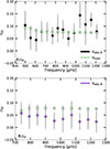 |
Fig. 5. Ratios r02 from test 2 for scenario A (top panel) and scenario B (bottom panel). The black points with error bars are computed from the observed frequencies and the green points correspond to the best-fit model. |
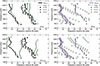 |
Fig. 6. Échelle diagram of the frequencies of the best models from test 2 (top row) and 3 (bottom row) including the ratios. The left columns show frequencies from scenario A, while the right columns show frequencies from scenario B. Circles represent modes ℓ = 0, triangles represent modes ℓ = 1, and diamonds represent modes with ℓ = 2. The black symbols with error bars indicate the observed frequencies and green symbols represent the model frequencies. The dotted gray line indicates the 56 μHZ frequency. |
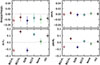 |
Fig. 7. Relative differences in surface gravity (top-left panel), radius (top-right panel), luminosity (bottom-left panel), and mass (bottom-right panel) between the observed values and our inferred results for the different surface corrections. The dotted line indicates where the relative difference is zero. |
The tests show that fitting frequencies yields higher χtotal2 values than fitting ratios. Among the surface corrections, BG141, KJ08, and SO15 show the largest χ2 values. Based solely on optimization, BG142 is preferred, yielding the smallest χtotal2, while neglecting surface corrections yields the worst results. However, comparing the inferred stellar mass to the expected value reveals a 6% relative difference for BG142, which is larger than the 2% deviation obtained with SO15 or without surface correction. The results with SO15 and without surface corrections reproduce the mass within 1σ, whereas BG142 reproduces it only within 3σ. The other parameters are generally consistent across the tests. The radius R is reproduced as expected, since it is used as a constraint. For log(g), all tests show similar relative differences of 1?2%. Regarding luminosity L, only the case without surface correction matches within a relative difference of 1%, while all other corrections show deviations greater than 10%, with BG142 performing worst.
The ratios are unaffected by surface effects and therefore serve as a reference to evaluate the mode identification in each test. Fig. 8 shows the differences between the model frequencies obtained with ratio-based optimization (orange symbols) and the best models computed with different surface corrections. Uncorrected frequencies are indicated by green symbols. In the upper panel, the model corrected with BG142 (blue symbols) shows the largest deviation compared to the ratio-based best model, with frequencies closer to the observed values. This result suggests that the BG142 surface correction overcorrects the individual frequencies. Although this may produce frequencies that better match the observations, the corresponding stellar properties deviate further from the expected values. We obtain the smallest deviation for the model computed with the SO15 correction (middle panel), whose inferred stellar mass is closest to the expected value, consistent with the fact that its individual frequencies are closer to the ratio-optimization model. In contrast, the model without surface correction (lower panel) shows frequencies closer to the observed values than to those of the ratio-based optimization model, indicating an undercorrection of the surface effects.
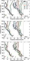 |
Fig. 8. Échelle diagram of the frequencies of the models resulting from the optimization procedure. The top panel shows the best model with the BG142 correction, the middle panel with the SO15 correction, and the bottom panel with no surface correction. Black symbols with error bars indicate the observed frequencies, green symbols represent the model frequencies without corrections, blue symbols represent the model frequencies with surface corrections, and the orange symbols represent the frequencies of the model constrained using ratios. Circles represent modes ℓ = 0, triangles represent modes with ℓ = 1, and diamonds represent modes ℓ = 2. The dotted gray line indicates the 56 μHZ frequency. |
Our results indicate that, for Procyon A, using frequency ratios in the fitting process yields the best results. The ratios provide tighter constraints on the stellar parameters and reproduce values close to the expected ones, particularly for the stellar mass. However, because not all stars have high-quality mode identifications, direct frequency fitting may still be required. Among the surface correction tests, BG142 fits the observational constraints most effectively but introduces inconsistencies likely related to the surface correction itself, which can shift the frequencies beyond the expected range. The SO15 correction achieves a more accurate recovery of the stellar parameters because, unlike BG14 and KJ08, it is calibrated on models covering a broader range of stellar properties rather than on the Sun. As expected, the case without surface corrections yields the highest χtotal2, but still provides reasonable stellar parameters, comparable to those obtained with SO15 or with the ratios. For Procyon A, we therefore recommend using ratios in the optimization process; if this is not feasible, the SO15 or no-surface-correction approaches offer the most reliable alternatives.
6. Conclusions
Procyon A is a benchmark F-type star with high-quality observations and well-characterized seismic spectra that provide detailed constraints on its internal structure. Its membership in a binary system ensures a well-determined stellar mass, making it particularly valuable for testing and validating stellar models of F-type stars.
Seismic analyses yield two possible scenarios for the individual frequencies: scenario A and scenario B. Although this was not the aim of this study, using frequency ratios, which are largely insensitive to surface effects, we find that scenario A is preferred. This scenario reproduces the observed stellar properties, especially the mass, and yields modeled frequencies that closely match the observations, consistent with previous studies (Doğan et al. 2010; Guenther et al. 2014; Compton et al. 2019). It is important to note that the use of ℓ = 1 modes prevents an accurate inference of the stellar properties. This is due to a glitch that appears at higher frequencies. This feature may reflect an incomplete description of the stellar structure, such as core rotation, internal magnetic fields, or an inadequate treatment of core overshoot. However, we note that White et al. (2012) preferred scenario B as the correct identification, which contradicts our conclusion. Missing physics in the models or an incorrect observational parameter identification could have led to the preference for scenario A over scenario B. To disentangle the two scenarios, new analyses and additional observations of this star are required.
The frequency ratios provide a useful reference for evaluating the agreement between the model and observed frequencies, as they remain largely unaffected by surface effects. This represents the best optimization process, yielding the smallest χ2 and most accurately reproducing the stellar properties, particularly the stellar mass of Procyon A. Testing different surface corrections allows us to minimize discrepancies with the observed constraints. However, although we could improve the optimization process, this would not improve the inference of stellar properties. Among the surface corrections, BG142 achieves the best fit to the observational constraints and the smallest χ2. However, it cannot accurately infer the stellar mass. This limitation likely arises because the BG14 correction, developed for the Sun, does not capture the surface physics of F-type stars. The SO15 and no-surface-correction cases yield higher χ2 values in the optimization process, but both reproduce the stellar mass of Procyon A. The improved performance of SO15 likely reflects its calibration over a broad range of stellar models rather than solar ones. The reasonable results from the no-surface-correction case, despite its high χ2, suggest that surface effects may be less significant for F-type stars or that other physical processes in the models compensate for the missing surface correction.
The results of the surface corrections can be compared with the core science objectives of the PLATO mission, which aims to achieve 15% uncertainty in the mass of solar-type stars. All estimated stellar masses fall within this range, with the largest deviations of 7% with the BG141 and KJ08 corrections. This indicates that BG142 is acceptable within these uncertainties, as it has a deviation of 6%. However, the deviations observed in some cases indicate areas where the surface-correction models may need refinement to better align with the expected stellar properties. This study focuses exclusively on Procyon A, so extending the analysis to a larger sample of F-type stars is necessary to fully understand the impact of surface corrections and determine the most appropriate prescriptions. Ultimately, improving our physical modeling of surface effects remains the best path forward.
Procyon A is a unique target, as it is one of the few F-type stars with a well-determined stellar mass, providing a strong constraint for stellar models. This makes it a valuable benchmark for improving the modeling of surface layers and for studying convective transport in the outer envelope. Additionally, it provides insights into the stellar interior. The presence of a glitch at high frequencies indicates incomplete modeling of the interior, which could arise from an inaccurate treatment of core overshoot, core rotation, or internal magnetic fields.
Acknowledgments
We acknowledge funding for the publication of the present manuscript and for the position of N. M. from the research theory grant ?Synergic tools for characterizing solar-like stars and habitability conditions of exoplanets” under the INAF national call for Fundamental Research 2023.
References
- Alecian, G., & LeBlanc, F. 2020, MNRAS, 498, 3420 [NASA ADS] [CrossRef] [Google Scholar]
- Arentoft, T., Kjeldsen, H., Bedding, T. R., et al. 2008, ApJ, 687, 1180 [NASA ADS] [CrossRef] [Google Scholar]
- Aufdenberg, J. P., Ludwig, H. G., & Kervella, P. 2005, ApJ, 633, 424 [Google Scholar]
- Ball, W. H., & Gizon, L. 2014, A&A, 568, A123 [NASA ADS] [CrossRef] [EDP Sciences] [Google Scholar]
- Bedding, T. R., Kjeldsen, H., Bouchy, F., et al. 2005, A&A, 432, L43 [NASA ADS] [CrossRef] [EDP Sciences] [Google Scholar]
- Bedding, T. R., Kjeldsen, H., Campante, T. L., et al. 2010, ApJ, 713, 935 [NASA ADS] [CrossRef] [Google Scholar]
- Bond, H. E., Gilliland, R. L., Schaefer, G. H., et al. 2015, ApJ, 813, 106 [Google Scholar]
- Borucki, W. J., Koch, D., Gibor, B., et al. 2010, Science, 327, 977 [CrossRef] [PubMed] [Google Scholar]
- Brown, T. M., Gilliland, R. L., Noyes, R. W., & Ramsey, L. W. 1991, ApJ, 368, 599 [Google Scholar]
- Ceillier, T., Ballot, J., Garcia, R. A., et al. 2011, arXiv e-prints [arXiv:1110.0307] [Google Scholar]
- Christensen-Dalsgaard, J., & Thompson, M. J. 1997, MNRAS, 284, 527 [NASA ADS] [Google Scholar]
- Christensen-Dalsgaard, J., Dappen, W., & Lebreton, Y. 1988, Nature, 336, 634 [Google Scholar]
- Christensen-Dalsgaard, J., Dappen, W., Ajukov, S. V., et al. 1996, Science, 272, 1286 [Google Scholar]
- Compton, D. L., Bedding, T. R., & Stello, D. 2019, MNRAS, 485, 560 [Google Scholar]
- Davies, G. R., Silva Aguirre, V., Bedding, T. R., et al. 2016, MNRAS, 456, 2183 [Google Scholar]
- Deal, M., Goupil, M. J., Cunha, M. S., et al. 2023, A&A, 673, A49 [NASA ADS] [CrossRef] [EDP Sciences] [Google Scholar]
- Deal, M., Goupil, M. J., Philidet, J., et al. 2025, A&A, 693, A240 [NASA ADS] [CrossRef] [EDP Sciences] [Google Scholar]
- Doğan, G., Bonanno, A., Bedding, T. R., et al. 2010, Astron. Nachr., 331, 949 [Google Scholar]
- Dziembowski, W. A., Paterno, L., & Ventura, R. 1988, A&A, 200, 213 [NASA ADS] [Google Scholar]
- Eggenberger, P., Carrier, F., Bouchy, F., & Blecha, A. 2004, A&A, 422, 247 [NASA ADS] [CrossRef] [EDP Sciences] [Google Scholar]
- Eggenberger, P., Carrier, F., & Bouchy, F. 2005, New A, 10, 195 [Google Scholar]
- Gaia Collaboration (Brown, A. G. A., et al.) 2021, A&A, 649, A1 [NASA ADS] [CrossRef] [EDP Sciences] [Google Scholar]
- Garcia, R. A., Ballot, J., Mathur, S., Salabert, D., & Regulo, C. 2010, arXiv e-prints [arXiv:1012.0494] [Google Scholar]
- Gatewood, G., & Han, I. 2006, AJ, 131, 1015 [Google Scholar]
- Girard, T. M., Wu, H., Lee, J. T., et al. 2000, AJ, 119, 2428 [Google Scholar]
- Guenther, D. B., Demarque, P., & Gruberbauer, M. 2014, ApJ, 787, 164 [NASA ADS] [CrossRef] [Google Scholar]
- Kjeldsen, H., Bedding, T. R., & Christensen-Dalsgaard, J. 2008, ApJ, 683, L175 [Google Scholar]
- LeBlanc, F., & Alecian, G. 2004, MNRAS, 352, 1329 [NASA ADS] [CrossRef] [Google Scholar]
- Lund, M. N., Silva Aguirre, V., Davies, G. R., et al. 2017, ApJ, 835, 172 [Google Scholar]
- Martić, M., Schmitt, J., Lebrun, J. C., et al. 1999, A&A, 351, 993 [Google Scholar]
- Michel, E., Baglin, A., Auvergne, M., et al. 2008, Science, 322, 558 [Google Scholar]
- Moedas, N., Bossini, D., Deal, M., & Cunha, M. S. 2024, A&A, 684, A113 [NASA ADS] [CrossRef] [EDP Sciences] [Google Scholar]
- Moedas, N., Deal, M., & Bossini, D. 2025, A&A, 695, A9 [NASA ADS] [CrossRef] [EDP Sciences] [Google Scholar]
- Paxton, B., Bildsten, L., Dotter, A., et al. 2011, ApJS, 192, 3 [Google Scholar]
- Paxton, B., Cantiello, M., Arras, P., et al. 2013, ApJS, 208, 4 [Google Scholar]
- Paxton, B., Marchant, P., Schwab, J., et al. 2015, ApJS, 220, 15 [Google Scholar]
- Paxton, B., Schwab, J., Bauer, E. B., et al. 2018, ApJS, 234, 34 [NASA ADS] [CrossRef] [Google Scholar]
- Paxton, B., Smolec, R., Schwab, J., et al. 2019, ApJS, 243, 10 [Google Scholar]
- Perdelwitz, V., Trifonov, T., Teklu, J. T., Sreenivas, K. R., & Tal-Or, L. 2024, A&A, 683, A125 [NASA ADS] [CrossRef] [EDP Sciences] [Google Scholar]
- Rauer, H., Aerts, C., & Cabrera, J. 2025, Exp. Astron., 59, 26 [Google Scholar]
- Rendle, B. M., Buldgen, G., Miglio, A., et al. 2019, MNRAS, 484, 771 [Google Scholar]
- Ricker, G. R. 2016, AGU Fall Meeting Abstracts, P13C-01 [Google Scholar]
- Roxburgh, I. W., & Vorontsov, S. V. 2003, A&A, 411, 215 [NASA ADS] [CrossRef] [EDP Sciences] [Google Scholar]
- Sonoi, T., Samadi, R., Belkacem, K., et al. 2015, A&A, 583, A112 [NASA ADS] [CrossRef] [EDP Sciences] [Google Scholar]
- Soubiran, C., Creevey, O. L., Lagarde, N., et al. 2024, A&A, 682, A145 [NASA ADS] [CrossRef] [EDP Sciences] [Google Scholar]
- Straka, C. W., Demarque, P., & Guenther, D. B. 2005, ApJ, 629, 1075 [CrossRef] [Google Scholar]
- Tassoul, M. 1980, ApJS, 43, 469 [Google Scholar]
- Verma, K., & Silva Aguirre, V. 2019, MNRAS, 489, 1850 [NASA ADS] [CrossRef] [Google Scholar]
- Verma, K., Raodeo, K., Basu, S., et al. 2019, MNRAS, 483, 4678 [Google Scholar]
- Walker, G., Matthews, J., Kuschnig, R., et al. 2003, PASP, 115, 1023 [Google Scholar]
- White, T. R., Bedding, T. R., Gruberbauer, M., et al. 2012, ApJ, 751, L36 [NASA ADS] [CrossRef] [Google Scholar]
All Tables
Relative and normalized differences of the inferred stellar properties for each test and for the two frequency scenarios.
Relative and normalized differences of stellar properties for tests of different surface-frequency corrections.
All Figures
|
Fig. 1. Kiel diagram showing computed evolutionary tracks with metallicity [M/H]i = 0.0 and Yi = 0.26 (solar composition) as solid gray lines. The star symbol marks the location of Procyon A in the diagram. The solid blue line represents the evolutionary track of the best model (circle symbol) from the r02 test, considering the radius in the inference of scenario A. |
| In the text | |
|
Fig. 2. Relative difference between the inferred and reference values (subscript r) obtained in test 1 for the two frequency sets (Scenarios A and B). The top-left panel shows the surface gravity, the top-right panel the surface radius, bottom-left panel the surface luminosity, and bottom-right panel the stellar mass. The dotted line indicates where the relative difference is zero. |
| In the text | |
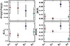 |
Fig. 3. Same as Fig. 2, but showing the relative differences obtained in test 2. |
| In the text | |
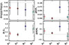 |
Fig. 4. Same as Fig. 2, but showing the relative differences obtained in test 3. |
| In the text | |
|
Fig. 5. Ratios r02 from test 2 for scenario A (top panel) and scenario B (bottom panel). The black points with error bars are computed from the observed frequencies and the green points correspond to the best-fit model. |
| In the text | |
|
Fig. 6. Échelle diagram of the frequencies of the best models from test 2 (top row) and 3 (bottom row) including the ratios. The left columns show frequencies from scenario A, while the right columns show frequencies from scenario B. Circles represent modes ℓ = 0, triangles represent modes ℓ = 1, and diamonds represent modes with ℓ = 2. The black symbols with error bars indicate the observed frequencies and green symbols represent the model frequencies. The dotted gray line indicates the 56 μHZ frequency. |
| In the text | |
|
Fig. 7. Relative differences in surface gravity (top-left panel), radius (top-right panel), luminosity (bottom-left panel), and mass (bottom-right panel) between the observed values and our inferred results for the different surface corrections. The dotted line indicates where the relative difference is zero. |
| In the text | |
|
Fig. 8. Échelle diagram of the frequencies of the models resulting from the optimization procedure. The top panel shows the best model with the BG142 correction, the middle panel with the SO15 correction, and the bottom panel with no surface correction. Black symbols with error bars indicate the observed frequencies, green symbols represent the model frequencies without corrections, blue symbols represent the model frequencies with surface corrections, and the orange symbols represent the frequencies of the model constrained using ratios. Circles represent modes ℓ = 0, triangles represent modes with ℓ = 1, and diamonds represent modes ℓ = 2. The dotted gray line indicates the 56 μHZ frequency. |
| In the text | |
Current usage metrics show cumulative count of Article Views (full-text article views including HTML views, PDF and ePub downloads, according to the available data) and Abstracts Views on Vision4Press platform.
Data correspond to usage on the plateform after 2015. The current usage metrics is available 48-96 hours after online publication and is updated daily on week days.
Initial download of the metrics may take a while.