| Issue |
A&A
Volume 706, February 2026
|
|
|---|---|---|
| Article Number | A141 | |
| Number of page(s) | 7 | |
| Section | The Sun and the Heliosphere | |
| DOI | https://doi.org/10.1051/0004-6361/202556660 | |
| Published online | 05 February 2026 | |
A self-consistent 3D magnetohydrodynamic model producing a solar blowout jet
1
Max-Planck Institute for Solar System Research (MPS) 37077 Göttingen, Germany
2
Institute for Solar Physics (KIS) Georges-Köhler-Allee 401A 79110 Freiburg, Germany
★ Corresponding author: This email address is being protected from spambots. You need JavaScript enabled to view it.
Received:
30
July
2025
Accepted:
21
December
2025
Abstract
Context. Solar blowout jets are a distinct subclass of ubiquitous extreme-ultraviolet (EUV) and X-ray coronal jets.
Aims. Most existing models of blowout jets prescribe initial magnetic-field configurations and apply ad hoc changes in the photosphere to trigger the jets. In contrast, we aim for a self-consistent magneto-convective description of the jet initiation.
Methods. We employed a 3D radiation magnetohydrodynamic (MHD) model of a solar coronal hole region using the MURaM code. The computational domain extends from the upper convection zone to the lower corona. We synthesized the emission in the EUV and X-ray for direct comparison with observations and examined the evolution of the magnetic-field structure of the event.
Results. In the simulation a twisted flux tube forms self-consistently, emerges through the surface, and interacts with the preexisting open field. Initially, the resulting jet is of the standard type with a narrow spire. The release of the twist into the open field causes a broadening of the jet spire, turning the jet into a blowout type. At the same time, this creates a fast heating front, propagating at the local Alfvén speed. The properties of the modeled jet closely match those of the observed blowout jets: a slow (∼180 km s−1) mass upflow and a fast (∼500 km s−1) propagating front form, the latter being a signature of the heating front. Also, the timing of the jet with respect to flux emergence and subsequent cancellation matches observations.
Conclusions. Near-surface magneto-convection self-consistently generates a twisted flux tube that emerges through the photosphere. The tube then interacts with the preexisting magnetic field by means of interchange reconnection. This transfers the twist to the open field and produces a blowout jet that matches the main characteristics of that found in observations.
Key words: magnetohydrodynamics (MHD) / Sun: corona / Sun: magnetic fields
© The Authors 2026
 Open Access article, published by EDP Sciences, under the terms of the Creative Commons Attribution License (https://creativecommons.org/licenses/by/4.0), which permits unrestricted use, distribution, and reproduction in any medium, provided the original work is properly cited.
This article is published in open access under the Subscribe to Open model.
Open Access funding provided by Max Planck Society.
1. Introduction
Solar coronal jets are collimated plasma outflows that have been extensively studied particularly since the soft X-ray observations of Yohkoh (e.g., Shibata et al. 1992; Shimojo et al. 1996). They are often observed in extreme-ultraviolet (EUV) wavelengths (e.g. Alexander & Fletcher 1999; Patsourakos et al. 2008; Doschek et al. 2010; Tian et al. 2012) and sometimes have chromospheric counterparts referred to as surges (e.g., Schmieder et al. 1995; Chae 2003; Liu & Kurokawa 2004; Chen et al. 2008). They typically have lengths of tens of megameters, widths of several megameters, and lifetimes of minutes in EUV or X-ray observations (e.g., Savcheva et al. 2007). Some coronal jets extend to several solar radii and are observed in white-light coronagraph images (e.g., Wang et al. 1998; Hong et al. 2013; Moore et al. 2015). For recent reviews on coronal jets, we refer to Raouafi et al. (2016) and Shen (2021).
Moore et al. (2010) suggested that coronal jets can be categorized into two classes – namely standard and blowout jets – based on their morphology. The spires of standard jets remain thin and narrow during their lifetime, while those of blowout jets broaden to the width of the jet bases and often present untwisting motions of helical structures (e.g., Shen et al. 2011; Chen et al. 2012). The morphology of jets can change between standard and blowout types during their lifetimes (Liu et al. 2011; Mandal et al. 2022). Blowout jets are often associated with eruptions of mini-filaments (e.g., Moore et al. 2013; Adams et al. 2014; Sterling et al. 2015; Joshi et al. 2018) and exhibit strong emission from cooler plasma observed in the 304 Å (e.g., Moore et al. 2010) and Lyα 1216 Å passbands (Long et al. 2023). Blowout jets seem to have two velocity components: a bulk mass flow at ∼200 km s−1 and a faster component at ∼700 km s−1 generally seen in channels imaging hotter plasma (e.g., X-ray). This is interpreted as signatures of Alfvén waves propagating with the jets (Cirtain et al. 2007; Long et al. 2023). Although the distinction between standard and blowout jets was originally introduced based on lower-resolution X-ray and EUV observations, higher-resolution EUV observations still reveal morphological differences. For example, most small-scale standard jets remain narrow and lack untwisting motions and mini-filament eruptions (e.g., Hou et al. 2021; Chitta et al. 2023). Therefore, we use the term blowout jet here to emphasize these specific characteristics, while recognizing that both types belong to the broader category of coronal jets.
Coronal jets are sometimes associated with flux emergence and/or cancellation (e.g., Shibata et al. 1992; Chifor et al. 2008; Young & Muglach 2014a,b; Panesar et al. 2016, 2018; Muglach 2021; Hou et al. 2021; Duan et al. 2024), which is often suggested to be a signature of magnetic reconnection. Magnetic extrapolations before jet events often reveal 3D null points at their base (e.g., Moreno-Insertis et al. 2008; Zhang et al. 2012) where breakout reconnection can occur and trigger coronal jets (e.g., Kumar et al. 2018, 2019; Kayshap et al. 2024).
To understand the formation mechanisms of coronal jets, various magnetohydrodynamic (MHD) simulations have been conducted. Earlier 2D models demonstrated that standard jets can be produced by magnetic reconnection between emerging flux and preexisting ambient magnetic field (e.g., Yokoyama & Shibata 1995, 1996). Building on this, one group of models is constructed with twisted flux ropes emerging from below the surface, in which subsequent magnetic reconnection between the newly emerged twisted field lines and overlaying background magnetic-field lines produces blowout jets (e.g., Archontis & Hood 2013; Moreno-Insertis & Galsgaard 2013; Fang et al. 2014). Another group of models begins with an initial 3D null-point magnetic configuration. Some of these models drive the magnetic field at the surface through rotating motions, producing twisted structures in the closed loops and injecting magnetic free energy into the system. Later on, instability-driven reconnection at the null point releases the stored energy and leads to blowout jets (e.g., Pariat et al. 2009, 2015; Szente et al. 2017; Karpen et al. 2017; Uritsky et al. 2017). Some models with similar initial magnetic structures impose shearing motions at the surface to form flux ropes that later undergo breakout reconnection and trigger twisted jets (e.g., Wyper et al. 2017, 2018a,b). In addition, data-driven models construct initial magnetic-field configuration through extrapolation, reproducing the eruptive phase by manually adjusting the magnetic (or electric) field in the photosphere (e.g., Cheung et al. 2015; Nayak et al. 2019) or by directly inserting flux ropes (e.g., Farid et al. 2022; Li et al. 2025).
In this study, we reproduce a blowout jet self-consistently in 3D time-dependent radiation MHD simulations, without prescribing any special magnetic-field configurations for the jet or manually inserting flux tubes. The jet naturally arises from magneto-convection in our simulation. We first compare the properties of the blowout jet in our model with those in observations and then investigate the underlying formation mechanisms driving the jet.
2. MHD model and methods
The simulation was constructed from a snapshot of a quiet Sun model using the MURaM code (Vögler et al. 2005; Rempel 2017), described in detail in Chen et al. (2025). The computational domain covers an area of 54 × 54 Mm2 in the horizontal directions with a grid size of ∼52.7 km. The model has a depth of 20 Mm, with a vertical grid spacing of 20 km. The initial snapshot reaches a height of ∼500 km above the surface, and we added a uniform vertical magnetic-field component of 5 G to replicate the flux imbalance in a coronal-hole region. After the simulation was saturated, we extended the model first to 6 Mm above the surface to form the transition region and then to 30 Mm to establish the corona. Afterward, we ran the simulation for an additional ∼10 hours, during which magnetograms and the full 3D data cubes were collected with cadences of ∼6 s and ∼6 min, respectively. The model was maintained by a small-scale dynamo, and we did not prescribe flux emergence or any particular magnetic-field structure except for the additional uniform 5 G added to the vertical magnetic-field component at the very beginning.
During the simulation run, a blowout jet was produced self-consistently. To better capture the jet dynamics, we restarted the simulation from the snapshot before the jet occurrence and collected outputs from our model at a 10 s cadence for 20 minutes. We define the time stamp of the first collected snapshot as t = 0 s.
To compare the model with observations, we synthesized emissions in three passbands: 304 Å from the Atmospheric Imaging Assembly (AIA, Lemen et al. 2012) on board Solar Dynamics Observatory, 174 Å from the Extreme Ultraviolet Imager (EUI, Rochus et al. 2020) on board Solar Orbiter, and Al-poly from the X-Ray Telescope (XRT, Golub et al. 2007) on board Hinode. Under the assumption of optically thin radiation, the emissivity at each voxel in a given passband is given by ne2Gi(ne, T), where ne and T are electron number density and temperature, and Gi(ne, T) is the contribution function, or kernel, of the passband. We integrated the emissivity along a defined line of sight (LOS) to calculate the intensity maps.
Although the emission in the AIA 304 Å passband in real observations is not optically thin, our approach can provide a reasonable proxy for the emission from plasma at ∼105 K. The synthesized EUI 174 Å and XRT Al-poly images represent emission from plasma at ∼106 K and ∼106.3 K, respectively. To avoid contamination from the emission by other bright structures along the LOS, we selected a small region containing the blowout jet when synthesizing intensity maps.
3. Results
3.1. Dynamics of the jet
We first present the temporal evolution of the jet in the EUI 174 Å passband in Fig. 1. At the beginning, the jet exhibits a narrow spire and presents a Y-shaped morphology. Several minutes later, the spire broadens to several megameters, comparable to the width of the jet base. Thus, the jet evolves from a standard- to a blowout-type eruption, similar to some events in observations (Liu et al. 2011). The jet lasts for about 10 minutes, and its emission signatures reach the top of the simulation domain, indicating that it can be traced to lengths of at least 30 Mm. These parameters are consistent with observational characteristics of blowout jets (Raouafi et al. 2016).
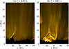 |
Fig. 1. Extreme UV images synthesized from a small region of the model showing two stages of the jet. Panel (a): Standard-jet phase. Panel (b): Same as panel (a) but five minutes later when the jet transitioned into the blowout-jet phase. Both images show the emission in the EUI 174 Å passband integrated along the y-axis. This represents a view at or near the solar limb of plasma at temperatures around 1 MK. See Sect. 3.1. |
In addition, we present synthesized images in AIA 304 Å and XRT Al-poly passbands during the blowout-jet phase in Fig. 2. The jet is clearly visible in all three passbands. In particular, it shows strong emission in the AIA 304 Å passband, with the 304 Å emission originating from a solid core of cool plasma. It demonstrates the presence of strong cool plasma within the jet. This also matches observations of the blowout jets (Moore et al. 2010).
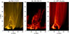 |
Fig. 2. Synthesized images of the blowout jet in different passbands. (a) Similar to Fig. 1, but around time t = 1000 s. (b–c) Similar to (a), but for AIA 304 Å and Hinode/XRT Al-poly passbands at the same time. An animation is available online. See Sect. 3.1. |
To further compare with observations, we placed three artificial slits at different heights and stacked the emission along these slits over time. This is similar to placing a slit on imaging data in observations to construct a space-time diagram from observations. The results are presented in Fig. 3. During the blowout-jet phase, the bright features in the space-time diagrams grow in size over time, as outlined by the dashed blue line in Fig. 3c, indicating radial expansion of the jet spire. In the meantime, bright threads within the jet spire move laterally from one side of the jet to the other due to untwisting motions, producing bright stripes in the space-time diagrams. One example is outlined by the dashed red line in Fig. 3b. Both the radial expansion and the untwisting patterns, similar to those seen in observations (e.g., Shen et al. 2011; Chen et al. 2012), are clearly visible in the diagrams at all heights. Untwisting patterns generally appear first at lower heights and subsequently at higher ones, indicating that the untwisting motion propagates upward along the jet. In addition, we calculated the radial expansion speed of the jet spire and the transverse (untwisting) speed of threads within the jet from the space–time diagrams. The radial expansion speed is approximately 36 km s−1, and the transverse component reaches up to 116 km s−1. These values are consistent with those reported by Shen et al. (2011). Here we selected one horizontal direction for comparison, and it is worth mentioning that choosing a different horizontal direction gives similar results.
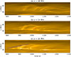 |
Fig. 3. Space-time diagrams across the jet spire at different heights. These represent the temporal evolution at a horizontal line along the x-direction placed within the jet spire. Panels (a)–(c) show the evolution at heights of 18, 14, and 10 Mm above the surface. The sloped red and blue lines in panels (b) and (c) indicate apparent speeds of 116 km s−1 (red) and 36 km s−1 (blue). See Sect. 3.1 for details. |
As a next step, we calculated the jet speeds in the vertical direction using synthesized EUI 174 Å and XRT Al-poly images. We integrated the emissivity of the two passbands horizontally for each snapshot and then stacked them to create the space-time diagrams shown in Fig. 4 a and c. This shows the (horizontally averaged) propagation of the jet in the vertical direction as a function of time. To highlight the propagation of the jet, we calculated running differences by subtracting the horizontally integrated emission of the previous snapshot (Δt = 10 s) from each snapshot and stacking the results into diagrams shown in Fig. 4 b and d. Based on these space-time diagrams, we estimated the jet speeds to be around 184 km s−1 in the EUI 174 Å passband and about 504 km s−1 in the XRT Al-poly passband. This is similar to the two components of the jet speed, as reported in observations (Long et al. 2023).
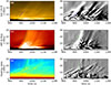 |
Fig. 4. Space-time diagrams along the vertical direction. These show the horizontally averaged vertical profile of the respective quantity as a function of time. From top to bottom: Evolution in EUI 174 Å (a–b), Hinode/XRT (c–d), and in heating rate (e–f). Left: Original value of the emissivity (a, c) and heating rate (e). Right: Respective running difference images (with a time delay of 10 s) simply to highlight the temporal changes. The dashed lines indicate apparent speeds of 184 km s−1 (a–b) and 504 km s−1 (c–f). See Sect. 3.1. |
The lower speed in the EUI 174 Å passband corresponds to bulk mass flows of the jet, while the higher speed in the XRT Al-poly passband corresponds to Alfvén speeds in the jet. However, the plasma velocity in and around the jet does not exceed 400 km s−1 during the entire lifetime of the jet, hence, the higher apparent speed component cannot be explained by a bulk mass flow. To investigate the origin of the high-speed component, we present a space-time diagram of the heating rates (the sum of Joule and viscous heating) along the vertical direction in Fig. 4e, similar to the plots for the EUI and XRT synthesized emission. This clearly shows an upward-propagating feature, similar to that seen in the XRT emission in panel (c), with a speed matching that found in the synthesized XRT Al-poly images. Therefore, the higher-speed component seen in the hotter channels can be attributed to heating fronts.
3.2. Magnetic origin of the jet
We present the temporal evolution of the magnetic flux in the photosphere beneath the jet in Fig. 5. Flux emergence first occurs, accompanied by the formation of small-scale mixed polarities modulated by the Parker instability (Parker 1966). The newly emerged opposite-polarity magnetic elements diverge and move apart by more than 5 Mm within about 10 minutes, indicating that the closed loops rise in height. Subsequently, flux cancellation among these newly emerged polarities occurs at the same locations. The jet appears approximately 10 minutes after the magnetic flux reaches its maximum, coinciding with the decreasing trends in both positive and negative magnetic flux. The delay between flux emergence and jet appearance occurs because the newly emerged magnetic flux requires tens of minutes to rise to coronal heights and establish a suitable magnetic configuration for reconnection, thereby producing signatures in coronal images.
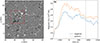 |
Fig. 5. Temporal evolution of the vertical magnetic-field component in the photosphere beneath the jet. (a) Zoomed-in FOV of the magnetogram beneath the jet. (b) Sums of the absolute values of positive (orange curve) and negative (blue curve) polarities in the red box outlined in (a). The vertical dashed gray line indicates the time of the magnetogram shown in (a). An animation is available online. See Sect. 3.2. |
The magnitudes of the changes in positive and negative magnetic flux are around 0.5 × 10¹⁹ Mx, which is similar to the values found in observations (Panesar et al. 2016). As a test, we slightly changed the location and size of the region used to calculate the magnetic flux (outlined by the red box in Fig. 5a) and found that this does not affect our conclusions.
Flux emergence and/or cancellation is generally considered to be a signature of magnetic reconnection in the solar atmosphere (e.g., Samanta et al. 2019). To examine the magnetic-field topology in and around the blowout jet, we traced magnetic-field lines from 80 seed points around the jet base in both backward and forward directions in space. For simplicity, we fixed the locations of the seed points when tracing the field lines for different snapshots.
Magnetic-field lines in two snapshots are presented in Fig. 6. The left panel corresponds to the standard stage, and the right panel shows the blowout stage. Initially, twisted closed loops emerge into the corona and reconnect with preexisting ambient background magnetic-field lines. During this phase, the closed loops continuously rise and expand, increasing in height before the onset of the jet. The jet originates at the interface between the closed and open field lines and appears as a standard jet, consistent with previous numerical studies (e.g., Shibata et al. 1992; Isobe et al. 2006). The region of high current density expands as the jet base broadens, without showing any clear rotational drift similar to that reported by Pariat et al. (2010). As the current sheet expands, reconnection between the twisted closed loops and the open field occurs across a wide area. The closed loops are opened and transfer their twist to the open field lines over an extended range at relatively low heights. Because the field lines at higher heights are nearly straight, magnetic tension allows the twist to propagate upward, driving the blowout jet characterized by untwisting motions and the lateral expansion of the jet spire. One feature is that the field lines within the jet spire during the blowout-jet phase are less well aligned compared to the standard-jet phase, as indicated by the white arrows in Fig. 6. This naturally explains the transition from the standard to the blowout stage.
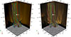 |
Fig. 6. Magnetic-field structure surrounding the jet. Left to right: Standard- and blowout-jet phases at the same times as in Fig. 1. In each panel the bottom shows a zoom-in of the magnetogram at the respective time. The synthesized EUI 174 Å images integrated over the x- and y-directions are depicted in the vertical slices of each 3D box. The colored lines represent the magnetic-field lines in and around the jet. The white arrows point to field lines in the jet spire that become misaligned during the blowout-jet phase, compared to the more aligned configuration during the standard phase. This indicates the untwisting motions likewise visible in the EUI 174 Å images on the vertical slices of the animation showing the temporal evolution. The animation is available online. See Sect. 3.2. |
We also applied the null-point detection method of Pallister et al. (2021) to identify magnetic nulls within the jet and found a null point throughout the standard-jet phase and the subsequent transition to the blowout-jet phase, i.e., when the jet base expands. The null exhibits chaotic motion and shifts back and forth within an area of ∼2 × 2 Mm2 in the xy-plane, without any clear rotational pattern. During the blowout-jet phase the null point disappears, likely because the fan-spine topology is destroyed.
4. Discussion
A blowout jet is self-consistently generated in our model, reproducing many observational features associated with this type of jet. By examining the magnetic-field structure in and around the jet during its lifetime, we find that the jet is triggered by interchange reconnection between newly emerged, twisted closed loops and neighboring open field lines.
In our model the twist in the emerging (magnetically closed) loops preceding the jet is built up in the convection zone prior to flux emergence, since no clear rotational or shearing flows are seen in the photosphere afterward. This behavior is quite different from previous numerical experiments where such surface motions play a key role in injecting the twist into the structure that produces the jet (e.g., Pariat et al. 2015; Wyper et al. 2017).
The mechanism we find here, i.e., a twisted magnetic structure emerging through the photosphere, is similar to that in previous MHD simulations of blowout jets, where a twisted flux rope was manually inserted to initiate flux emergence and the jet (Archontis & Hood 2013; Moore et al. 2013; Fang et al. 2014). However, the flux emergence in our model occurs self-consistently without the necessity to implant a flux rope beneath the surface by hand. During the interchange magnetic reconnection with the preexisting (open) magnetic field, twist is transferred from closed to open field lines, which drives the untwisting motion in the jet spire.
Long et al. (2023) reported that blowout jets can exhibit two velocity components; they interpreted the slower component as mass flow and the faster one as the untwisting of newly formed field lines during reconnection. Similar high-speed components in coronal jets were reported in X-ray observations by Cirtain et al. (2007), which the authors interpreted as signatures of Alfvén waves associated with the jets. Previous numerical studies have demonstrated that magnetic reconnection producing coronal jets can generate Alfvénic waves (e.g., Lynch et al. 2014; Pariat et al. 2015; Lee et al. 2015; Wyper et al. 2022; Yang et al. 2025). Nonlinear Alfvénic disturbances can steepen to form shocks and current sheets, where energy is dissipated, thereby contributing to local heating (e.g., Hollweg et al. 1982; Cohen & Kulsrud 1974).
Our model successfully and self-consistently reproduces the two velocity components. The fast component (∼500 km s−1) corresponds to heating fronts rather than real mass motion. This is supported by the fact that the speed of the fast component roughly matches the local Alfvén speed within the jet. This is because magnetic perturbations, triggered by reconnection, travel along the field lines at the Alfvén speed, and the associated current sheets apparently propagate with these disturbances. The subsequent dissipation of the current sheets through Joule and viscous heating produces an apparent heating front. As in any other 3D MHD model of the solar corona, the magnetic Reynolds and Prandtl numbers in our simulation are substantially different from those in the real corona. Still, the magnetic disturbances will cascade and steepen to small scales and dissipate energy at such fronts (Hollweg et al. 1982; Cohen & Kulsrud 1974; van der Holst et al. 2014). The details of the dissipation might be different, but the overall physical picture remains robust. Hence, our results are consistent with earlier studies in which heating fronts have been invoked to interpret the high speeds observed in network jets in transition-region images (De Pontieu et al. 2017; Tian et al. 2014).
Although the blowout jet in our model reproduces many observed features, we did not reproduce small-scale structures identified in some observations, such as mini-filament eruptions (e.g., Sterling et al. 2015). We did not find strong shearing motions along a polarity inversion line, and the emerging flux does not seem to form a filament channel. Therefore, a mini-filament is unlikely to form in our model. This mismatch might also be attributed to the treatment of the chromosphere in our model. Our current simulations do not include a proper treatment of the chromosphere (Przybylski et al. 2022), which could play an important role in filament formation.
In our model, flux cancellation at the jet base occurs mostly among newly emerged magnetic patches. We examined several cancellation events and found that the regions of enhanced current density are mainly located in the photosphere and extend up to heights of ∼500 km. The associated downflows also originate from heights of a few hundreds kilometers. This indicates that many of the cancellation events in our model correspond to magnetic reconnection in the photosphere. Furthermore, we noticed that some canceling small-scale magnetic elements are initially connected to the major positive and negative magnetic concentrations. This implies that these reconnection events help rearrange the magnetic footpoint connectivity, thereby modulating the fan-spine topology.
However, in observations, some events appear associated with flux cancellation only, without clear signatures of flux emergence (e.g., Adams et al. 2014). Still, we consider it possible that, in these earlier studies, the emergence of new magnetic flux prior to the final cancellation during the jet event was simply missed in the observations. For some events studied by Panesar et al. (2016), magnetic patches with opposite polarities approach each other prior to flux cancellation, which typically lasts for several hours before the jet onset. In our simulation, the jet was launched ∼10 minutes after flux cancellation began. Thus, the timescale for the accumulation of magnetic free energy in our model is significantly shorter than that in observations.
More generally, it remains a matter of debated whether flux cancellation plays a key role in jet triggering. For example, Kumar et al. (2019) found that only about 20% of coronal-hole jets are associated with flux cancellation, while Tang et al. (2021) showed that blowout jets can be triggered by such external disturbances at coronal heights as nearby eruptions. Thus, our model represents a class of coronal jets in which flux emergence and subsequent cancellation together drive the jet. In this scenario, flux cancellation is not necessarily the trigger itself but can arise naturally from magnetic reconnection between the newly emerged and preexisting magnetic fields.
Another observed jet feature missing from our model is the presence of small-scale blobs (e.g., Shen et al. 2017; Kumar et al. 2019; Mandal et al. 2022; Long et al. 2023; Cheng et al. 2023). The blobs are often interpreted as signatures of plasmoids triggered during magnetic reconnection (Biskamp 2000). Previous high-resolution simulations of magnetic reconnection successfully reproduced plasmoids in jets (Wyper et al. 2016; Ni et al. 2017; Peter et al. 2019; Nóbrega-Siverio et al. 2025). Therefore, increasing the spatial resolution of our simulations might be necessary to capture plasmoids or blob-like features within the jet.
5. Conclusions
In this study, we presented a blowout jet that is self-consistently generated in a 3D radiation MHD model of a solar coronal-hole region. To compare it with observations, we synthesized images in the AIA 304 Å, EUI 174 Å, and XRT Al-poly passbands. The width, length, and lifetime of the jet are consistent with observed properties. Furthermore, the jet in our model exhibits strong emission from cool plasma in the synthesized AIA 304 Å images and clear untwisting motions in the synthesized coronal images. We identified two distinct speed components in the jet: a slower component (∼180 km s−1) corresponding to mass flows and a faster component (∼500 km s−1) associated with heating fronts. In addition, flux cancellation occurring beneath the jet base was detected, consistent with some observations. All these characteristics closely match with observations.
Because of the good match with observations, we assume that the underlying physics in our model provide a good representation of what occurs on the real Sun. We examined the temporal evolution of magnetic-field structures in and around the jet and found that the jet is triggered by magnetic interchange reconnection between newly emerged, twisted closed loops and ambient open magnetic-field lines. The twisted loops are generated self-consistently through the near-surface convection in the Sun and then emerge through the photosphere. This does not exclude the possibility that surface motions may also create this twisted magnetic structure that initiates the blowout jet. Still, our model demonstrates one clear way in which such twisted structures form, emerge, and subsequently produce jets. During the reconnection process, twist is transferred from closed loops to open magnetic-field lines, driving magnetic disturbances associated with untwisting motions and heating fronts. In conclusion, our model presents a self-consistent description of how the twisted pre-jet structures form and emerge, how they interact with the existing open magnetic field, and how this process ultimately produces the blowout jet at the base of the solar wind.
Data availability
Movies associated to Figs. 2, 5, 6 are available at https://www.aanda.org
Acknowledgments
Y.C. acknowledges funding provided by the Alexander von Humboldt Foundation. The work of Y.C., D.P., and S.M. was funded by the Federal Ministry for Economic Affairs and Climate Action (BMWK) through the German Space Agency at DLR based on a decision of the German Bundestag (Funding code: 50OU2201). LPC gratefully acknowledges funding by the European Union (ERC, ORIGIN, 101039844). We gratefully acknowledge the computational resources provided by the Cobra and Raven supercomputer systems of the Max Planck Computing and Data Facility (MPCDF) in Garching, Germany.
References
- Adams, M., Sterling, A. C., Moore, R. L., & Gary, G. A. 2014, ApJ, 783, 11 [NASA ADS] [CrossRef] [Google Scholar]
- Alexander, D., & Fletcher, L. 1999, Sol. Phys., 190, 167 [NASA ADS] [CrossRef] [Google Scholar]
- Archontis, V., & Hood, A. W. 2013, ApJ, 769, L21 [Google Scholar]
- Biskamp, D. 2000, Magnetic Reconnection in Plasmas, 3 [Google Scholar]
- Chae, J. 2003, ApJ, 584, 1084 [NASA ADS] [CrossRef] [Google Scholar]
- Chen, H. D., Jiang, Y. C., & Ma, S. L. 2008, A&A, 478, 907 [NASA ADS] [CrossRef] [EDP Sciences] [Google Scholar]
- Chen, H.-D., Zhang, J., & Ma, S.-L. 2012, Res. Astron. Astrophys., 12, 573 [Google Scholar]
- Chen, Y., Peter, H., Przybylski, D., Iijima, H., & Pradeep Chitta, L. 2025, A&A, 702, L4 [NASA ADS] [CrossRef] [EDP Sciences] [Google Scholar]
- Cheng, X., Priest, E. R., Li, H. T., et al. 2023, Nat. Commun., 14, 2107 [Google Scholar]
- Cheung, M. C. M., De Pontieu, B., Tarbell, T. D., et al. 2015, ApJ, 801, 83 [Google Scholar]
- Chifor, C., Isobe, H., Mason, H. E., et al. 2008, A&A, 491, 279 [NASA ADS] [CrossRef] [EDP Sciences] [Google Scholar]
- Chitta, L. P., Zhukov, A. N., Berghmans, D., et al. 2023, Science, 381, 867 [NASA ADS] [CrossRef] [Google Scholar]
- Cirtain, J. W., Golub, L., Lundquist, L., et al. 2007, Science, 318, 1580 [Google Scholar]
- Cohen, R. H., & Kulsrud, R. M. 1974, Phys. Fluids, 17, 2215 [NASA ADS] [CrossRef] [Google Scholar]
- De Pontieu, B., Martínez-Sykora, J., & Chintzoglou, G. 2017, ApJ, 849, L7 [Google Scholar]
- Doschek, G. A., Landi, E., Warren, H. P., & Harra, L. K. 2010, ApJ, 710, 1806 [NASA ADS] [CrossRef] [Google Scholar]
- Duan, Y., Tian, H., Chen, H., et al. 2024, ApJ, 962, L38 [Google Scholar]
- Fang, F., Fan, Y., & McIntosh, S. W. 2014, ApJ, 789, L19 [NASA ADS] [CrossRef] [Google Scholar]
- Farid, S. I., Savcheva, A., Tassav, S., & Reeves, K. K. 2022, ApJ, 938, 150 [Google Scholar]
- Golub, L., DeLuca, E., Austin, G., et al. 2007, Sol. Phys., 243, 63 [NASA ADS] [CrossRef] [Google Scholar]
- Hollweg, J. V., Jackson, S., & Galloway, D. 1982, Sol. Phys., 75, 35 [NASA ADS] [CrossRef] [Google Scholar]
- Hong, J.-C., Jiang, Y.-C., Yang, J.-Y., et al. 2013, Res. Astron. Astrophys., 13, 253 [Google Scholar]
- Hou, Z., Tian, H., Berghmans, D., et al. 2021, ApJ, 918, L20 [NASA ADS] [CrossRef] [Google Scholar]
- Isobe, H., Miyagoshi, T., Shibata, K., & Yokoyama, T. 2006, PASJ, 58, 423 [Google Scholar]
- Joshi, N. C., Nishizuka, N., Filippov, B., Magara, T., & Tlatov, A. G. 2018, MNRAS, 476, 1286 [Google Scholar]
- Karpen, J. T., DeVore, C. R., Antiochos, S. K., & Pariat, E. 2017, ApJ, 834, 62 [Google Scholar]
- Kayshap, P., Karpen, J. T., & Kumar, P. 2024, Sol. Phys., 299, 88 [Google Scholar]
- Kumar, P., Karpen, J. T., Antiochos, S. K., et al. 2018, ApJ, 854, 155 [NASA ADS] [CrossRef] [Google Scholar]
- Kumar, P., Karpen, J. T., Antiochos, S. K., et al. 2019, ApJ, 873, 93 [NASA ADS] [CrossRef] [Google Scholar]
- Lee, E. J., Archontis, V., & Hood, A. W. 2015, ApJ, 798, L10 [Google Scholar]
- Lemen, J. R., Title, A. M., Akin, D. J., et al. 2012, Sol. Phys., 275, 17 [Google Scholar]
- Li, Z. F., Guo, J. H., Cheng, X., et al. 2025, A&A, 696, L2 [NASA ADS] [CrossRef] [EDP Sciences] [Google Scholar]
- Liu, Y., & Kurokawa, H. 2004, ApJ, 610, 1136 [Google Scholar]
- Liu, C., Deng, N., Liu, R., et al. 2011, ApJ, 735, L18 [NASA ADS] [CrossRef] [Google Scholar]
- Long, D. M., Chitta, L. P., Baker, D., et al. 2023, ApJ, 944, 19 [NASA ADS] [CrossRef] [Google Scholar]
- Lynch, B. J., Edmondson, J. K., & Li, Y. 2014, Sol. Phys., 289, 3043 [Google Scholar]
- Mandal, S., Chitta, L. P., Peter, H., et al. 2022, A&A, 664, A28 [NASA ADS] [CrossRef] [EDP Sciences] [Google Scholar]
- Moore, R. L., Cirtain, J. W., Sterling, A. C., & Falconer, D. A. 2010, ApJ, 720, 757 [Google Scholar]
- Moore, R. L., Sterling, A. C., Falconer, D. A., & Robe, D. 2013, ApJ, 769, 134 [Google Scholar]
- Moore, R. L., Sterling, A. C., & Falconer, D. A. 2015, ApJ, 806, 11 [NASA ADS] [CrossRef] [Google Scholar]
- Moreno-Insertis, F., & Galsgaard, K. 2013, ApJ, 771, 20 [Google Scholar]
- Moreno-Insertis, F., Galsgaard, K., & Ugarte-Urra, I. 2008, ApJ, 673, L211 [Google Scholar]
- Muglach, K. 2021, ApJ, 909, 133 [NASA ADS] [CrossRef] [Google Scholar]
- Nayak, S. S., Bhattacharyya, R., Prasad, A., et al. 2019, ApJ, 875, 10 [Google Scholar]
- Ni, L., Zhang, Q.-M., Murphy, N. A., & Lin, J. 2017, ApJ, 841, 27 [Google Scholar]
- Nóbrega-Siverio, D., Joshi, R., Sola-Viladesau, E., Berghmans, D., & Lim, D. 2025, A&A, 702, A188 [NASA ADS] [CrossRef] [EDP Sciences] [Google Scholar]
- Pallister, R., Wyper, P. F., Pontin, D. I., DeVore, C. R., & Chiti, F. 2021, ApJ, 923, 163 [NASA ADS] [CrossRef] [Google Scholar]
- Panesar, N. K., Sterling, A. C., Moore, R. L., & Chakrapani, P. 2016, ApJ, 832, L7 [Google Scholar]
- Panesar, N. K., Sterling, A. C., & Moore, R. L. 2018, ApJ, 853, 189 [NASA ADS] [CrossRef] [Google Scholar]
- Pariat, E., Antiochos, S. K., & DeVore, C. R. 2009, ApJ, 691, 61 [Google Scholar]
- Pariat, E., Antiochos, S. K., & DeVore, C. R. 2010, ApJ, 714, 1762 [NASA ADS] [CrossRef] [Google Scholar]
- Pariat, E., Dalmasse, K., DeVore, C. R., Antiochos, S. K., & Karpen, J. T. 2015, A&A, 573, A130 [NASA ADS] [CrossRef] [EDP Sciences] [Google Scholar]
- Parker, E. N. 1966, ApJ, 145, 811 [NASA ADS] [CrossRef] [Google Scholar]
- Patsourakos, S., Pariat, E., Vourlidas, A., Antiochos, S. K., & Wuelser, J. P. 2008, ApJ, 680, L73 [NASA ADS] [CrossRef] [Google Scholar]
- Peter, H., Huang, Y. M., Chitta, L. P., & Young, P. R. 2019, A&A, 628, A8 [NASA ADS] [CrossRef] [EDP Sciences] [Google Scholar]
- Przybylski, D., Cameron, R., Solanki, S. K., et al. 2022, A&A, 664, A91 [NASA ADS] [CrossRef] [EDP Sciences] [Google Scholar]
- Raouafi, N. E., Patsourakos, S., Pariat, E., et al. 2016, Space Sci. Rev., 201, 1 [Google Scholar]
- Rempel, M. 2017, ApJ, 834, 10 [Google Scholar]
- Rochus, P., Auchère, F., Berghmans, D., et al. 2020, A&A, 642, A8 [NASA ADS] [CrossRef] [EDP Sciences] [Google Scholar]
- Samanta, T., Tian, H., Yurchyshyn, V., et al. 2019, Science, 366, 890 [NASA ADS] [CrossRef] [Google Scholar]
- Savcheva, A., Cirtain, J., Deluca, E. E., et al. 2007, PASJ, 59, S771 [Google Scholar]
- Schmieder, B., Shibata, K., van Driel-Gesztelyi, L., & Freeland, S. 1995, Sol. Phys., 156, 245 [NASA ADS] [CrossRef] [Google Scholar]
- Shen, Y. 2021, Proc. R. Soc. Lond. Ser. A, 477, 217 [NASA ADS] [Google Scholar]
- Shen, Y., Liu, Y., Su, J., & Ibrahim, A. 2011, ApJ, 735, L43 [NASA ADS] [CrossRef] [Google Scholar]
- Shen, Y., Liu, Y. D., Su, J., Qu, Z., & Tian, Z. 2017, ApJ, 851, 67 [NASA ADS] [CrossRef] [Google Scholar]
- Shibata, K., Ishido, Y., Acton, L. W., et al. 1992, PASJ, 44, L173 [Google Scholar]
- Shimojo, M., Hashimoto, S., Shibata, K., et al. 1996, PASJ, 48, 123 [Google Scholar]
- Sterling, A. C., Moore, R. L., Falconer, D. A., & Adams, M. 2015, Nature, 523, 437 [NASA ADS] [CrossRef] [Google Scholar]
- Szente, J., Toth, G., Manchester, W. B., IV., et al. 2017, ApJ, 834, 123 [NASA ADS] [CrossRef] [Google Scholar]
- Tang, Z., Shen, Y., Zhou, X., et al. 2021, ApJ, 912, L15 [Google Scholar]
- Tian, H., McIntosh, S. W., Wang, T., et al. 2012, ApJ, 759, 144 [Google Scholar]
- Tian, H., DeLuca, E. E., Cranmer, S. R., et al. 2014, Science, 346, 1255711 [Google Scholar]
- Uritsky, V. M., Roberts, M. A., DeVore, C. R., & Karpen, J. T. 2017, ApJ, 837, 123 [NASA ADS] [CrossRef] [Google Scholar]
- van der Holst, B., Sokolov, I. V., Meng, X., et al. 2014, ApJ, 782, 81 [Google Scholar]
- Vögler, A., Shelyag, S., Schüssler, M., et al. 2005, A&A, 429, 335 [Google Scholar]
- Wang, Y. M., Sheeley, N. R., Jr., Socker, D. G., et al. 1998, ApJ, 508, 899 [NASA ADS] [CrossRef] [Google Scholar]
- Wyper, P. F., DeVore, C. R., Karpen, J. T., & Lynch, B. J. 2016, ApJ, 827, 4 [NASA ADS] [CrossRef] [Google Scholar]
- Wyper, P. F., Antiochos, S. K., & DeVore, C. R. 2017, Nature, 544, 452 [Google Scholar]
- Wyper, P. F., DeVore, C. R., & Antiochos, S. K. 2018a, ApJ, 852, 98 [Google Scholar]
- Wyper, P. F., DeVore, C. R., Karpen, J. T., Antiochos, S. K., & Yeates, A. R. 2018b, ApJ, 864, 165 [NASA ADS] [CrossRef] [Google Scholar]
- Wyper, P. F., DeVore, C. R., Antiochos, S. K., et al. 2022, ApJ, 941, L29 [NASA ADS] [CrossRef] [Google Scholar]
- Yang, L., He, J., Feng, X., et al. 2025, ApJ, 982, L25 [Google Scholar]
- Yokoyama, T., & Shibata, K. 1995, Nature, 375, 42 [Google Scholar]
- Yokoyama, T., & Shibata, K. 1996, PASJ, 48, 353 [Google Scholar]
- Young, P. R., & Muglach, K. 2014a, PASJ, 66, S12 [Google Scholar]
- Young, P. R., & Muglach, K. 2014b, Sol. Phys., 289, 3313 [Google Scholar]
- Zhang, Q. M., Chen, P. F., Guo, Y., Fang, C., & Ding, M. D. 2012, ApJ, 746, 19 [NASA ADS] [CrossRef] [Google Scholar]
All Figures
|
Fig. 1. Extreme UV images synthesized from a small region of the model showing two stages of the jet. Panel (a): Standard-jet phase. Panel (b): Same as panel (a) but five minutes later when the jet transitioned into the blowout-jet phase. Both images show the emission in the EUI 174 Å passband integrated along the y-axis. This represents a view at or near the solar limb of plasma at temperatures around 1 MK. See Sect. 3.1. |
| In the text | |
|
Fig. 2. Synthesized images of the blowout jet in different passbands. (a) Similar to Fig. 1, but around time t = 1000 s. (b–c) Similar to (a), but for AIA 304 Å and Hinode/XRT Al-poly passbands at the same time. An animation is available online. See Sect. 3.1. |
| In the text | |
|
Fig. 3. Space-time diagrams across the jet spire at different heights. These represent the temporal evolution at a horizontal line along the x-direction placed within the jet spire. Panels (a)–(c) show the evolution at heights of 18, 14, and 10 Mm above the surface. The sloped red and blue lines in panels (b) and (c) indicate apparent speeds of 116 km s−1 (red) and 36 km s−1 (blue). See Sect. 3.1 for details. |
| In the text | |
|
Fig. 4. Space-time diagrams along the vertical direction. These show the horizontally averaged vertical profile of the respective quantity as a function of time. From top to bottom: Evolution in EUI 174 Å (a–b), Hinode/XRT (c–d), and in heating rate (e–f). Left: Original value of the emissivity (a, c) and heating rate (e). Right: Respective running difference images (with a time delay of 10 s) simply to highlight the temporal changes. The dashed lines indicate apparent speeds of 184 km s−1 (a–b) and 504 km s−1 (c–f). See Sect. 3.1. |
| In the text | |
|
Fig. 5. Temporal evolution of the vertical magnetic-field component in the photosphere beneath the jet. (a) Zoomed-in FOV of the magnetogram beneath the jet. (b) Sums of the absolute values of positive (orange curve) and negative (blue curve) polarities in the red box outlined in (a). The vertical dashed gray line indicates the time of the magnetogram shown in (a). An animation is available online. See Sect. 3.2. |
| In the text | |
|
Fig. 6. Magnetic-field structure surrounding the jet. Left to right: Standard- and blowout-jet phases at the same times as in Fig. 1. In each panel the bottom shows a zoom-in of the magnetogram at the respective time. The synthesized EUI 174 Å images integrated over the x- and y-directions are depicted in the vertical slices of each 3D box. The colored lines represent the magnetic-field lines in and around the jet. The white arrows point to field lines in the jet spire that become misaligned during the blowout-jet phase, compared to the more aligned configuration during the standard phase. This indicates the untwisting motions likewise visible in the EUI 174 Å images on the vertical slices of the animation showing the temporal evolution. The animation is available online. See Sect. 3.2. |
| In the text | |
Current usage metrics show cumulative count of Article Views (full-text article views including HTML views, PDF and ePub downloads, according to the available data) and Abstracts Views on Vision4Press platform.
Data correspond to usage on the plateform after 2015. The current usage metrics is available 48-96 hours after online publication and is updated daily on week days.
Initial download of the metrics may take a while.